wradlib Documentation - Bitbucket
wradlib Documentation - Bitbucket
wradlib Documentation - Bitbucket

Create successful ePaper yourself
Turn your PDF publications into a flip-book with our unique Google optimized e-Paper software.
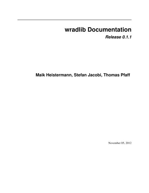
<strong>wradlib</strong> <strong>Documentation</strong><br />
Release 0.1.1<br />
Maik Heistermann, Stefan Jacobi, Thomas Pfaff<br />
November 05, 2012
CONTENTS<br />
1 Getting Started 3<br />
1.1 Installing Python . . . . . . . . . . . . . . . . . . . . . . . . . . . . . . . . . . . . . . . . . . . . . 3<br />
1.2 Installing <strong>wradlib</strong> . . . . . . . . . . . . . . . . . . . . . . . . . . . . . . . . . . . . . . . . . . . . . 3<br />
1.3 Dependencies . . . . . . . . . . . . . . . . . . . . . . . . . . . . . . . . . . . . . . . . . . . . . . . 4<br />
1.4 Community . . . . . . . . . . . . . . . . . . . . . . . . . . . . . . . . . . . . . . . . . . . . . . . . 5<br />
2 Tutorials 7<br />
2.1 A typical workflow for radar-based rainfall estimation . . . . . . . . . . . . . . . . . . . . . . . . . 7<br />
2.2 Supported radar data formats . . . . . . . . . . . . . . . . . . . . . . . . . . . . . . . . . . . . . . . 13<br />
2.3 Read and plot raw DWD radar data . . . . . . . . . . . . . . . . . . . . . . . . . . . . . . . . . . . 16<br />
2.4 Converting reflectivities . . . . . . . . . . . . . . . . . . . . . . . . . . . . . . . . . . . . . . . . . 22<br />
2.5 Integration of precipitation rates (Accumulation) . . . . . . . . . . . . . . . . . . . . . . . . . . . . 27<br />
2.6 Clutter correction . . . . . . . . . . . . . . . . . . . . . . . . . . . . . . . . . . . . . . . . . . . . . 29<br />
2.7 Attenuation correction . . . . . . . . . . . . . . . . . . . . . . . . . . . . . . . . . . . . . . . . . . 33<br />
3 Library Reference 35<br />
3.1 Raw Data I/O . . . . . . . . . . . . . . . . . . . . . . . . . . . . . . . . . . . . . . . . . . . . . . . 35<br />
3.2 Reading BUFR Files . . . . . . . . . . . . . . . . . . . . . . . . . . . . . . . . . . . . . . . . . . . 38<br />
3.3 Data Transformation . . . . . . . . . . . . . . . . . . . . . . . . . . . . . . . . . . . . . . . . . . . 39<br />
3.4 Z-R Conversions . . . . . . . . . . . . . . . . . . . . . . . . . . . . . . . . . . . . . . . . . . . . . 40<br />
3.5 Georeferencing . . . . . . . . . . . . . . . . . . . . . . . . . . . . . . . . . . . . . . . . . . . . . . 41<br />
3.6 Interpolation . . . . . . . . . . . . . . . . . . . . . . . . . . . . . . . . . . . . . . . . . . . . . . . 47<br />
3.7 Data Quality . . . . . . . . . . . . . . . . . . . . . . . . . . . . . . . . . . . . . . . . . . . . . . . 51<br />
3.8 Composition . . . . . . . . . . . . . . . . . . . . . . . . . . . . . . . . . . . . . . . . . . . . . . . 53<br />
3.9 Clutter Identification . . . . . . . . . . . . . . . . . . . . . . . . . . . . . . . . . . . . . . . . . . . 55<br />
3.10 Filling Missing Values . . . . . . . . . . . . . . . . . . . . . . . . . . . . . . . . . . . . . . . . . . 57<br />
3.11 Vertical Profile of Reflectivity (VPR) . . . . . . . . . . . . . . . . . . . . . . . . . . . . . . . . . . 57<br />
3.12 Attenuation Correction . . . . . . . . . . . . . . . . . . . . . . . . . . . . . . . . . . . . . . . . . . 58<br />
3.13 Gage adjustment . . . . . . . . . . . . . . . . . . . . . . . . . . . . . . . . . . . . . . . . . . . . . 64<br />
3.14 Verification . . . . . . . . . . . . . . . . . . . . . . . . . . . . . . . . . . . . . . . . . . . . . . . . 79<br />
3.15 Visualisation . . . . . . . . . . . . . . . . . . . . . . . . . . . . . . . . . . . . . . . . . . . . . . . 86<br />
3.16 Utility functions . . . . . . . . . . . . . . . . . . . . . . . . . . . . . . . . . . . . . . . . . . . . . 90<br />
4 Development Setup 93<br />
4.1 <strong>Documentation</strong> Setup . . . . . . . . . . . . . . . . . . . . . . . . . . . . . . . . . . . . . . . . . . 93<br />
5 Team 95<br />
5.1 Developers . . . . . . . . . . . . . . . . . . . . . . . . . . . . . . . . . . . . . . . . . . . . . . . . 95<br />
5.2 Contributers . . . . . . . . . . . . . . . . . . . . . . . . . . . . . . . . . . . . . . . . . . . . . . . 95<br />
i
5.3 Users . . . . . . . . . . . . . . . . . . . . . . . . . . . . . . . . . . . . . . . . . . . . . . . . . . . 95<br />
6 Indices and tables 97<br />
Bibliography 99<br />
Python Module Index 101<br />
Python Module Index 103<br />
ii
<strong>wradlib</strong> <strong>Documentation</strong>, Release 0.1.1<br />
The <strong>wradlib</strong> project has been initiated in order facilitate the use of weather radar data as well as to provide a common<br />
platform for research on new algorithms. <strong>wradlib</strong> is an open source library which is well documented and easy to use.<br />
It is written in the free programming language Python.<br />
Note: Please cite <strong>wradlib</strong> as Heistermann, M., Jacobi, S., and Pfaff, T.: Technical Note: An open source library for<br />
processing weather radar data (<strong>wradlib</strong>), Hydrol. Earth Syst. Sci. Discuss., 9, 12333-12356, doi:10.5194/hessd-9-<br />
12333-2012, 2012<br />
Weather radar data is potentially useful in meteorology, hydrology and risk management. Its ability to provide information<br />
on precipitation with high spatio-temporal resolution over large areas makes it an invaluable tool for short term<br />
weather forecasting or flash flood forecasting.<br />
<strong>wradlib</strong> is designed to assist you in the most important steps of processing weather radar data. These may include:<br />
reading common data formats, georeferencing, converting reflectivity to rainfall intensity, identifying and correcting<br />
typical error sources (such as clutter or attenuation) and visualising the data.<br />
This documentation is under steady development. It provides a complete library reference as well as a set of tutorials<br />
which will get you started in working with <strong>wradlib</strong>.<br />
CONTENTS 1
<strong>wradlib</strong> <strong>Documentation</strong>, Release 0.1.1<br />
2 CONTENTS
CHAPTER<br />
ONE<br />
GETTING STARTED<br />
1.1 Installing Python<br />
In order to run <strong>wradlib</strong>, you need to have a Python interpreter installed on your local computer. <strong>wradlib</strong> will be guaranteed<br />
to work with a particular Python version, however, we will not guarantee upward or downward compatibility<br />
at the moment. The current version of <strong>wradlib</strong> is designed to be used with Python 2.7, but most features are also<br />
known to work under Python 2.6.<br />
<strong>wradlib</strong> was not designed to be a self-contained library. Besides extensive use of Numpy and Scipy, you might need<br />
to install additional libraries before you can use <strong>wradlib</strong>. See Dependencies for a full list of dependencies. Under<br />
Linux, the Python interpreter is usually pre-installed and installation of additional packages as well as dependency<br />
management is supposed to be easy.<br />
Under Windows operating systems, we strongly recommend to install a Python distribution such as<br />
Python(x,y) (http://code.google.com/p/pythonxy) which will contain most of the required packages. Go to<br />
http://code.google.com/p/pythonxy/wiki/Downloads, and select one of the Mirrors. Download the latest distribution<br />
(currently Python(x,y)-2.7.2.3.exe and install it. We recommend to use the full installation mode.<br />
When installing Python(x,y), make sure you choose “All Users” under the “Install for” menu component!<br />
Test the integrity of your Python installation by opening a console window and typing python. The console should<br />
show the Python version and a Python command prompt. Type<br />
>>> exit()<br />
in order to exit the Python environment.<br />
1.2 Installing <strong>wradlib</strong><br />
Download the source from https://bitbucket.org/<strong>wradlib</strong>/<strong>wradlib</strong> via the get source button and extract it to any<br />
location on your computer. Inside the extracted folder, open a console window (on the same directory level as the<br />
setup.py file) and execute:<br />
>>> python setup.py install<br />
This way, the <strong>wradlib</strong> package will be installed under the Python site-packages directory and will thus be available for<br />
import.<br />
Test the integrity of your <strong>wradlib</strong> installation by opening a console window and typing python. The Python prompt<br />
should appear. Then type<br />
3
<strong>wradlib</strong> <strong>Documentation</strong>, Release 0.1.1<br />
>>> import <strong>wradlib</strong><br />
If everything is ok, nothing will happen. If the <strong>wradlib</strong> package is not found by the interpreter, you will get<br />
>>> import <strong>wradlib</strong><br />
ImportError: No module named <strong>wradlib</strong><br />
Check whether your Python installation directory contains the subdirectory /Lib/sitepackages/<strong>wradlib</strong>/<strong>wradlib</strong> and the<br />
corresponding source files. If the <strong>wradlib</strong> directory is not there, execute python setup.py install, again, and<br />
inspect the screen output if any helpful error messages are reported.<br />
You may receive other ImportErrors if required packages are missing. Please make sure the required packages are<br />
installed (see Dependencies).<br />
Attention: In order to use <strong>wradlib</strong> for decoding BUFR files (see Supported radar data formats), the installation (via<br />
python setup.py install) tries to compile and build the OPERA BUFR software (which is included in the<br />
<strong>wradlib</strong> source). This part of the installation has the potential to cause some trouble and was only tested on Windows<br />
7 machines, yet. The process requires gcc and make. Both are pre-installed on most Linux machines, and can be<br />
installed on Windows using the MinGW compiler suite. If you are using Python(x,y), gcc and mingw32-make<br />
should already be available on your machine! You can check this by opening a console window and typing gcc<br />
--version and mingw32-make --version. For Linux, the required makefile is available and we hope that<br />
the installation process works. But we never tested it! Please give us your feedback how it works under Linux by<br />
sending an e-mail to <strong>wradlib</strong>-users@googlegroups.com or by raising an issue.<br />
Beyond this issue, <strong>wradlib</strong> is intended to support at least Windows and Linux platforms, but it was tested only on<br />
Windows, yet. If you discover any platform issues on Linux, please do not hesitate to raise an issue.<br />
1.3 Dependencies<br />
<strong>wradlib</strong> was not designed to be a self-contained library. Besides extensive use of Numpy and Scipy, <strong>wradlib</strong> uses<br />
additional libraries, which you will need to install before you can use <strong>wradlib</strong>. Note that all libraries marked with a<br />
(*) are not contained in the Python(x,y) distribution and thus have to be definitely installed manually.<br />
For Windows users: If possible, we will link binary installer files for the libraries below. However, installers are not<br />
always available. In this case, you have to install from source. For pure Python packages, this is easy. Just extract the<br />
source, open a console window on the same level that contains the setup.py file and execute:<br />
python setup.py install<br />
• basemap (*): Download installer at http://sourceforge.net/projects/matplotlib/files/matplotlib-toolkits/basemap-<br />
1.0.2/<br />
• h5py<br />
• matplotlib<br />
• netCDF4<br />
• numpy<br />
• numpydoc (*): Download source at http://pypi.python.org/pypi/numpydoc and install via python setup.py install<br />
• pylab<br />
• pyproj (*): Download installer at http://code.google.com/p/pyproj/downloads<br />
• scipy<br />
4 Chapter 1. Getting Started
<strong>wradlib</strong> <strong>Documentation</strong>, Release 0.1.1<br />
1.4 Community<br />
<strong>wradlib</strong> is intended to be a community effort, and community needs communication. The key communication platform<br />
for <strong>wradlib</strong> is the <strong>wradlib</strong>-users mailing list and forum. Through this forum, you can help to improve <strong>wradlib</strong><br />
by reporting bugs, proposing enhancements, or by contributing code snippets (in any programming language) and<br />
documentation of algorithms. You can also ask other users and developers for help, or use your own knowledge and<br />
experience to help other users. We strongly encourage you to subscribe to this list. Check it out!<br />
1.4. Community 5
<strong>wradlib</strong> <strong>Documentation</strong>, Release 0.1.1<br />
6 Chapter 1. Getting Started
CHAPTER<br />
TWO<br />
TUTORIALS<br />
The tutorials should give an idea how the individual functions of <strong>wradlib</strong> can be used for weather radar processing.<br />
For additional help to certain functions also consider to have look at the code examples distributed with the source<br />
code.<br />
2.1 A typical workflow for radar-based rainfall estimation<br />
Raw, unprocessed reflectivity products can already provide useful visual information about the spatial distribution<br />
of rainfall fields. However, in order to use weather radar observations for quantitative studies (e.g. in hydrological<br />
modelling or for assimilation into Numerical Weather Prediction models), the data has to be carefully processed<br />
in order to account for typical errors sources such as ground echoes (clutter), attenuation of the radar signal, or<br />
uncertainties in the Z/R relationship. Moreover, it might be necessary to transfer the data from polar coordinates to<br />
Cartesian grids, or to combine observations from different radar locations in overlapping areas on a common grid<br />
(composition). And in the end, you would typically like to visualise the spatial rainfall distribution on a map. Many<br />
users also need to quantify the potential error (uncertainty) of their data-based rainfall estimation.<br />
These are just some steps that might be necessary in order to make radar data useful in a specific quantitative application<br />
environment. All steps together are typically referred to as a radar data processing chain. <strong>wradlib</strong> was designed to<br />
support you in establishing your own processing chain, suited to your specific requirements. In the following, we will<br />
provide an outline of a typical processing chain, step-by-step. You might not need all steps for your own workflow,<br />
or you might need steps which are not yet included here. Consider this just as an example. We will not go into detail<br />
for each step in this section, but refer to more detailed tutorials (if available) or the corresponding entry in the library<br />
reference. Most of the steps have a corresponding <strong>wradlib</strong> module. In order to access the functions of <strong>wradlib</strong>, you<br />
have to import <strong>wradlib</strong> in your Python console:<br />
>>> import <strong>wradlib</strong><br />
If you have trouble with that import, please head back to the Getting Started section.<br />
Note: The code used in this tutorial can be found in the file wradib/examples/typical_workflow.py of<br />
the <strong>wradlib</strong> distribution. The corresponding example data is stored in <strong>wradlib</strong>/examples/data.<br />
Warning: Be aware that applying an algorithm for error correction does not guarantee that the error is totally<br />
removed. Error correction procedures are suceptible to errors, too. Not only might they fail to remove the error.<br />
They might also introduce new errors. The trade-off between costs (introduction of new errors) and benefits (error<br />
reduction) can turn out differently for different locations, different points in time, or different rainfall situations.<br />
7
<strong>wradlib</strong> <strong>Documentation</strong>, Release 0.1.1<br />
2.1.1 Reading the data<br />
The binary encoding of many radar products is a major obstacle for many potential radar users. Often, decoder software<br />
is not easily available. <strong>wradlib</strong> support a couple of formats such as the OPERA BUFR and hdf5 implementations,<br />
NetCDF, and some formats used by the Germany Weather Service. We seek to continuously enhance the range of<br />
supported formats.<br />
The basic data type used in <strong>wradlib</strong> is a multi-dimensional array, the numpy.ndarray. Such an array might e.g. represent<br />
a polar or Cartesian grid, or a series of rain gage observations. Metadata are normally managed as Python dictionaries.<br />
In order to read the content of a data file into a numpy array, you would normally use the wradib.io module. In the<br />
following example, a local PPI from the German Weather Service, a DX file, is read:<br />
>>> data, metadata = <strong>wradlib</strong>.io.readDX("DX_sample_file")<br />
>>> <strong>wradlib</strong>.vis.polar_plot(data) # simple diagnostic plot<br />
The metadata object can be inspected via keywords. The data object contains the actual data, in this case a polar<br />
grid with 360 azimuth angles and 128 range bins.<br />
See Also:<br />
Get more info in the section Supported radar data formats and in the library reference section Raw Data I/O.<br />
2.1.2 Clutter removal<br />
Clutter are non-precipitation echos. They are caused by the radar beam hitting objects on the earth’s surface (e.g.<br />
mountain or hill tops, houses, wind turbines) or in the air (e.g. airplanes, birds). These objects can potentially cause<br />
high reflectivities due large scattering cross sections. Static clutter, if not efficiently removed by Doppler filters, can<br />
cause permanent echos which could introduce severe bias in quantitative applications. Thus, an efficient identification<br />
and removal of clutter is mandatory e.g. for hydrological studies. Clutter removal can be based on static maps or<br />
dynamic filters. Normally, static clutter becomes visible more clearly in rainfall accumulation maps over periods of<br />
weeks or months. We recommend such accumulations to create static clutter maps which can in turn be used to remove<br />
the static clutter from an image and fill the resulting gaps by interpolation. In the following example, the clutter filter<br />
published by Gabella and Notarpietro ([Gabella2002]) is applied to the single radar sweep of the above example.<br />
>>> clutter = <strong>wradlib</strong>.clutter.filter_gabella(data, tr1=12, n_p=6, tr2=1.1)<br />
>>> <strong>wradlib</strong>.vis.polar_plot(clutter,title=’Clutter Map’,colormap=pl.cm.gray)<br />
The resulting Boolean array clutter indicates the position of clutter. It can be used to interpolate the values at those<br />
positons from non-clutter values, as shown in the following line:<br />
>>> data_no_clutter = <strong>wradlib</strong>.ipol.interpolate_polar(data, clutter)<br />
It is generally recommended to remove the clutter before e.g. gridding the data because this might smear the clutter<br />
signal over multiple grid cells, and result into a decrease in identifiability.<br />
See Also:<br />
Get more info in the section Clutter correction and in the library reference section Clutter Identification.<br />
2.1.3 Attenuation correction<br />
Attenuation by wet radome and by heavy rainfall can cause serious underestimation of rainfall for C-Band and X-<br />
Band devices. For such radar devices, situations with heavy rainfall require a correction of attenuation effects. The<br />
general approach with single-polarized radars is to use a recursive gate-by-gate approach. See Kraemer and Verworn<br />
([Kraemer2008]) for an introduction to this concept. Basically, the specific attenuation k of the first range gate is<br />
computed via a so-called k-Z relationship. Based on k, the reflectivity of the second range gate is corrected and then<br />
used to compute the specific attenuation for the second range gate (and so on). The concept was first introduced by<br />
8 Chapter 2. Tutorials
<strong>wradlib</strong> <strong>Documentation</strong>, Release 0.1.1<br />
Hitchfeld and Bordan ([Hitschfeld1954]). Its main drawback is its suceptibility to instable behaviour. <strong>wradlib</strong> provides<br />
a different implementations which address this problem. One example is the algorithm published by Kraemer and<br />
Verworn ([Kraemer2008]):<br />
>>> pia = <strong>wradlib</strong>.atten.correctAttenuationKraemer(data_no_clutter)<br />
>>> data_attcorr = data_no_clutter + pia<br />
The first line computes the path integrated attenuation pia for each radar bin. The second line line uses pia to correct<br />
the reflectivity values. Let’s inspect the effect of attenuation correction for an azimuth angle of 65?:<br />
>>> import pylab as pl<br />
>>> pl.plot(data_attcorr[65], label="attcorr")<br />
>>> pl.plot(data_no_clutter[65], label="no attcorr")<br />
>>> pl.xlabel("km")<br />
>>> pl.ylabel("dBZ")<br />
>>> pl.legend()<br />
>>> pl.show()<br />
See Also:<br />
Get more info in the library reference section Attenuation Correction. Here you will learn to know the algorithms<br />
available for attenuation correction and how to manipulate their behaviour by using additonal keyword arguments.<br />
2.1.4 Vertical Profile of Reflectivity<br />
Not yet available - implementation is ongoing.<br />
2.1.5 Conversion of reflectivity into rainfall<br />
Reflectivity (Z) and precipitation rate (R) can be related in form of a power law R=a*Z**b. The parameters a and b<br />
depend on the type of precipitation in terms of drop size distribution and water temperature. Before applying the Z-R<br />
relationship, we need to convert from dBZ to Z:<br />
>>> R = <strong>wradlib</strong>.zr.z2r( <strong>wradlib</strong>.trafo.idecibel(data_attcorr) )<br />
The above line uses the default parameters parameters a=200 and b=1.6 for the Z-R relationship. In order to<br />
compute a rainfall depth from rainfall intensity, we have to specify an integration interval in seconds. In this example,<br />
we choos fove minutes (300 s), corresponding to the sweep return interval:<br />
>>> depth = <strong>wradlib</strong>.trafo.r2depth(R, 300)<br />
See Also:<br />
Get more info in the section Converting reflectivities and in the library reference sections Z-R Conversions and Data<br />
Transformation. Here you will learn about the effects of the Z-R parameters a and b.<br />
2.1.6 Rainfall accumulation<br />
For many applications, accumulated rainfall depths over specific time intervals are required, e.g. hourly or daily<br />
accumulations. <strong>wradlib</strong> supports the corresponding datetime operations. In the following example, we will use a<br />
synthetic time series of 5 minute intervals. Just imagine we have repeated the above procedure for one day of fiveminute<br />
sweeps and combined the arrays of rainfall depth in a 3-dimensional array of shape (number of time<br />
steps, number of azimuth angles, number of range gates). Now we want to ocompute hourly<br />
accumulations:<br />
2.1. A typical workflow for radar-based rainfall estimation 9
<strong>wradlib</strong> <strong>Documentation</strong>, Release 0.1.1<br />
>>> import numpy as np<br />
>>> sweep_times = <strong>wradlib</strong>.util.from_to("2012-10-26 00:00:00", "2012-10-27 00:00:00", 300)<br />
>>> depths_5min = np.random.uniform(size=(len(sweep_times)-1, 360, 128))<br />
>>> hours = <strong>wradlib</strong>.util.from_to("2012-10-26 00:00:00", "2012-10-27 00:00:00", 3600)<br />
>>> depths_hourly= <strong>wradlib</strong>.util.aggregate_in_time(depths_5min, sweep_times, hours, func=’sum’)<br />
Check the shape and values of your resulting array for plausibility:<br />
>>> print depths_hourly.shape<br />
(24, 360, 128)<br />
>>> print depths_hourly.mean().round()<br />
6.0<br />
See Also:<br />
Get more info in the library reference section Utility functions.<br />
2.1.7 Georeferencing and projection<br />
In order to define the horizontal and vertical position of the radar bins, we need to retrieve the corresponding 3-<br />
dimensional coordinates in terms of latitude, longitude and altitude. This information is required e.g. if the positions<br />
should be plotted on a map. It is also required for constructing CAPPIs. The position of a radar bin in 3-dimensional<br />
space depends on the position of the radar device, the elevation angle of the radar beam, as well as the azimuth angle<br />
and the range of a bin. For the sample data used above, the posiiton of the radar device is the Feldberg in Germany<br />
(47.8744, 8.005, 1517):<br />
>>> import numpy as np<br />
>>> radar_location = (47.8744, 8.005, 1517) # (lat, lon, alt) in decimal degree and meters<br />
>>> elevation = 0.5 # in degree<br />
>>> azimuths = np.arange(0,360) # in degrees<br />
>>> ranges = np.arange(0, 128000., 1000.) # in meters<br />
>>> polargrid = np.meshgrid(ranges, azimuths)<br />
>>> lat, lon, alt = <strong>wradlib</strong>.georef.polar2latlonalt(polargrid[0], polargrid[1], elevation, radar_locat<br />
<strong>wradlib</strong> supports the projection of geographical coordinates (lat/lon) to a Cartesian reference system. Basically, you<br />
have to provide a string which represents the projection - based on the proj.4 library. You can look up projection<br />
strings, but for some projections, <strong>wradlib</strong> helps you to define a projection string. In the following example, the target<br />
projection is Gauss-Krueger (zone 3):<br />
>>> gk3 = <strong>wradlib</strong>.georef.create_projstr("gk", zone=3)<br />
>>> x, y = <strong>wradlib</strong>.georef.project(lat, lon, gk3)<br />
See Also:<br />
Get more info in the library reference section Georeferencing.<br />
2.1.8 Gridding<br />
Assume you would like to transfer the rainfall intensity from the above example (Conversion of reflectivity into rainfall)<br />
from polar coordinates to a Cartesian grid, or to an arbitrary set of irregular points in space (e.g. centroids of<br />
sub-catchments). You already retrieved the Cartesian coordinates of the radar bins in the previous section (Georeferencing<br />
and projection). Now you only need to define the target coordinates (e.g. a grid) and apply the togrid<br />
function of the <strong>wradlib</strong>.comp module. In this example, we want our grid only to represent the South-West sector<br />
of our radar circle on a 100 x 100 grid. First, we define the target grid coordinates (these must be an array of 100x100<br />
rows with one coordinate pair each):<br />
10 Chapter 2. Tutorials
<strong>wradlib</strong> <strong>Documentation</strong>, Release 0.1.1<br />
>>> xgrid = np.linspace(x.min(), x.mean(), 100)<br />
>>> ygrid = np.linspace(y.min(), y.mean(), 100)<br />
>>> grid_xy = np.meshgrid(xgrid, ygrid)<br />
>>> grid_xy = np.vstack((grid_xy[0].ravel(), grid_xy[1].ravel())).transpose()<br />
Now we transfer the polar data to the grid and mask out invalid values for plotting (values outside the radar circle<br />
receive NaN):<br />
>>> gridded = <strong>wradlib</strong>.comp.togrid(xy, grid_xy, 128000., np.array([x.mean(), y.mean()]), data.ravel(),<br />
>>> gridded = np.ma.masked_invalid(gridded).reshape((len(xgrid), len(ygrid)))<br />
>>> <strong>wradlib</strong>.vis.cartesian_plot(gridded, x=xgrid, y=ygrid, classes=range(0,70,5), unit="dBZ")<br />
See Also:<br />
Get more info about the function <strong>wradlib</strong>.comp.togrid.<br />
2.1.9 Adjustment by rain gage observations<br />
Adjustment normally refers to using rain ggage observations on the ground to correct for errors in the radar-based<br />
rainfall estimatin. Goudenhooftd and Delobbe [Goudenhoofdt2009] provide an excellent overview of adjustment<br />
procedures. A typical approach is to quantify the error of the radar-based rainfall estimate at the rain gage locations,<br />
assuming the rain gage observation to be accurate. The error can be assumed to be additive, multiplicative, or a mixture<br />
of both. Most approaches assume the error to be heterogeneous in space. Hence, the error at the rain gage locations<br />
will be interpolated to the radar bin (or grid) locations and then used to adjust (correct) the raw radar rainfall estimates.<br />
In the following example, we will use an illustrative one-dimensional example with synthetic data (just imagine radar<br />
rainfall estimates and rain gage observations along one radar beam).<br />
First, we create the synthetic “true” rainfall (truth).<br />
>>> import numpy as np<br />
>>> radar_coords = np.arange(0,101)<br />
>>> truth = np.abs(1.5+np.sin(0.075*radar_coords)) + np.random.uniform(-0.1,0.1,len(radar_coords))<br />
The radar rainfall estimate radar is then computed by imprinting a multiplicative error on truth and adding<br />
some noise.<br />
>>> error = 0.75 + 0.015*radar_coords<br />
>>> radar = error * truth + np.random.uniform(-0.1,0.1,len(radar_coords))<br />
Synthetic gage observations obs are then created by selecting arbitrary “true” values.<br />
>>> obs_coords = np.array([5,10,15,20,30,45,65,70,77,90])<br />
>>> obs = truth[obs_coords]<br />
Now we adjust the radar rainfall estimate by using the gage observations. First, you create an “adjustment object”<br />
from the approach you want to use for adjustment. After that, you can call the object with the actual data that is to be adjusted.<br />
Here, we use a multiplicative error model with spatially heterogenous error (see <strong>wradlib</strong>.adjust.AdjustMultiply).<br />
>>> adjuster = <strong>wradlib</strong>.adjust.AdjustMultiply(obs_coords, radar_coords, nnear_raws=3)<br />
>>> adjusted = adjuster(obs, radar)<br />
Let’s compare the truth, the radar rainfall estimate and the adjusted product:<br />
>>> import pylab as pl<br />
>>> pl.plot(radar_coords, truth, ’k-’, label="True rainfall", linewidth=2.)<br />
>>> pl.xlabel("Distance (km)")<br />
>>> pl.ylabel("Rainfall intensity (mm/h)")<br />
>>> pl.plot(radar_coords, radar, ’k-’, label="Raw radar rainfall", linewidth=2., linestyle="dashed")<br />
2.1. A typical workflow for radar-based rainfall estimation 11
<strong>wradlib</strong> <strong>Documentation</strong>, Release 0.1.1<br />
>>> pl.plot(obs_coords, obs, ’o’, label="Gage observation", markersize=10.0, markerfacecolor="grey")<br />
>>> pl.plot(radar_coords, adjusted, ’-’, color="green", label="Multiplicative adjustment", linewidth=<br />
>>> pl.legend(prop={’size’:12})<br />
>>> pl.show()<br />
See Also:<br />
Get more info in the library reference section Gage adjustment. There, you will also learn how to use the built-in<br />
cross-validation in order to evaluate the performance of the adjustment approach.<br />
2.1.10 Verification and quality control<br />
Typically, radar-based precipitation estimation and the effectiveness of the underlying correction and adjustment methods<br />
are verified by comparing the results against rain gauge observations on the ground. <strong>wradlib</strong>.verify provides procedures<br />
not only to extract the radar values at specific gauge locations, but also a set of error metrics which are computed<br />
from gage observations and the corresponding radar-based precipitation estimates (including standard metrics such<br />
as RMSE, mean error, Nash-Sutcliffe Efficiency). In the following, we will illustrate the usage of error metrics by<br />
comparing the “true” rainfall against the raw and adjusted radar rainfall estimates from the above example:<br />
>>> raw_error = <strong>wradlib</strong>.verify.ErrorMetrics(truth, radar)<br />
>>> adj_error = <strong>wradlib</strong>.verify.ErrorMetrics(truth, adjusted)<br />
Error metrics can be reported e.g. as follows:<br />
>>> raw_error.report()<br />
>>> adj_error.report()<br />
See Also:<br />
Get more info in the library reference section Verification.<br />
2.1.11 Visualisation and mapping<br />
In the above sections Reading the data, Clutter removal, and Gridding you already saw examples of the <strong>wradlib</strong>’s<br />
plotting capabilities.<br />
See Also:<br />
Get more info in the library reference section Visualisation.<br />
2.1.12 Data export to other applications<br />
Once you created a dataset which meets your requirements, you might want to export it to other applications or<br />
archives. <strong>wradlib</strong> does not favour or spupport a specific output format. Basically, you have all the freedom of choice<br />
offered by Python and its packages in order to export your data. Arrays can be stored as text or binary files by using<br />
numpy functions. You can use the package NetCDF4 to write NetCDF files, and the packages h5py or PyTables<br />
to write hdf5 files. At a later stage of development, <strong>wradlib</strong> might support a standardized data export by using the<br />
OPERA’s BUFR or hdf5 data model (see Supported radar data formats). Of course, you can also export data as<br />
images. See Visualisation for some options.<br />
Export your data array as a text file:<br />
>>> np.savetxt("mydata.txt", data)<br />
Or as a gzip-compressed text file:<br />
12 Chapter 2. Tutorials
<strong>wradlib</strong> <strong>Documentation</strong>, Release 0.1.1<br />
>>> np.savetxt("mydata.gz", data)<br />
Or as a NetCDF file:<br />
>>> import netCDF4<br />
>>> rootgrp = netCDF4.Dataset(’test.nc’, ’w’, format=’NETCDF4’)<br />
>>> sweep_xy = rootgrp.createGroup(’sweep_xy’)<br />
>>> dim_azimuth = sweep_xy.createDimension(’azimuth’, None)<br />
>>> dim_range = sweep_xy.createDimension(’range’, None)<br />
>>> azimuths_var = sweep_xy.createVariable(’azimuths’,’i4’,(’azimuth’,))<br />
>>> ranges_var = sweep_xy.createVariable(’ranges’,’f4’,(’range’,))<br />
>>> dBZ_var = sweep_xy.createVariable(’dBZ’,’f4’,(’azimuth’,’range’,))<br />
>>> azimuths_var[:] = np.arange(0,360)<br />
>>> ranges_var[:] = np.arange(0, 128000., 1000.)<br />
>>> dBZ_var[:] = data<br />
You can easily add metadata to the NetCDF file on different group levels:<br />
>>> rootgrp.bandwith = "C-Band"<br />
>>> sweep_xy.datetime = "2012-11-02 10:15:00"<br />
>>> rootgrp.close()<br />
Note: An example for hdf5 export will follow.<br />
2.1.13 References<br />
2.2 Supported radar data formats<br />
The binary encoding of many radar products is a major obstacle for many potential radar users. Often, decoder software<br />
is not easily available. In case formats are documented, the implementation of decoders is a major programming effort.<br />
This tutorial provides an overview of the data formats currently supported by <strong>wradlib</strong>. We seek to continuously enhance<br />
the range of supported formats, so this document is only a snapshot. If you need a specific file format to be supported<br />
by <strong>wradlib</strong>, please raise an issue of type enhancement. You can provide support by adding documents which help to<br />
decode the format, e.g. format reference documents or software code in other languages for decoding the format.<br />
At the moment, supported format means that the radar format can be read and further processed by <strong>wradlib</strong>. Normally,<br />
<strong>wradlib</strong> will return an array of data values and a dictionary of metadata - if the file contains any. <strong>wradlib</strong> does not<br />
support encoding to any specific file formats, yet! This might change in the future, but it is not a priority. However,<br />
you can use Python’s netCDF4 or h5py packages to encode the results of your analysis to standard self-describing<br />
file formats such as netCDF or hdf5. If you have Python(x,y) installed on your machine, these packages are readily<br />
available to you.<br />
In the following, we will provide an overview of file formats which can be currently read by <strong>wradlib</strong>. Reading weather<br />
radar files is done via the Raw Data I/O module. There you will find a complete function reference. So normally, you<br />
will start by:<br />
import <strong>wradlib</strong>.io as io<br />
2.2.1 German Weather Service: DX format<br />
The German Weather Service uses the DX file format to encode local radar sweeps. DX data are in polar coordinates.<br />
The naming convention is as follows: raa00-dx_--—bin<br />
or raa00-dx_--—bin. Read and plot raw DWD radar<br />
2.2. Supported radar data formats 13
<strong>wradlib</strong> <strong>Documentation</strong>, Release 0.1.1<br />
data provides an extensive introduction into working with DX data. For now, we would just like to know how to read<br />
the data:<br />
data, metadata = io.readDX("mydrive:/path/to/my/file/filename")<br />
Here, data is a two dimensional array of shape (number of azimuth angles, number of range gates). This means that<br />
the number of rows of the array corresponds to the number of azimuth angles of the radar sweep while the number of<br />
columns corresponds to the number of range gates per ray.<br />
2.2.2 German Weather Service: RADOLAN (quantitative) composit<br />
The quantitative composite format of the DWD (German Weather Service) was established in the course of the<br />
RADOLAN project. Most quantitative composite products from the DWD are distributed in this format, e.g. the<br />
R-series (RX, RY, RH, RW, ...), the S-series (SQ, SH, SF, ...), and the E-series (European quantitative composite, e.g.<br />
EZ, EH, EB). Please see the composite format description for a full reference and a full table of products (unfortunately<br />
only in German language).<br />
Currently, the RADOLAN composites have a spatial resolution of 1km x 1km, with the national composits (R- and<br />
S-series) being 900 x 900 grids, and the European composits 1500 x 1400 grids. The projection is polar-stereographic.<br />
The products can be read by the following function:<br />
data, metadata = io.read_RADOLAN_composite("mydrive:/path/to/my/file/filename")<br />
Here, data is a two dimensional integer array of shape (number of rows, number of columns). Different product<br />
types might need different levels of postprocessing, e.g. if the product contains rain rates or accumulations, you<br />
will normally have to divide data by factor 10. metadata is again a dictionary which provides metadata from the<br />
files header section, e.g. using the keys producttype, datetime, intervalseconds, nodataflag. Masking the NoData (or<br />
missing) values can be done by:<br />
import numpy as np<br />
maskeddata = np.ma.masked_equal(data, attrs["nodataflag"])<br />
2.2.3 OPERA BUFR<br />
The Binary Universal Form for the Representation of meteorological data (BUFR) is a binary data format maintained<br />
by the World Meteorological Organization (WMO). The BUFR format was adopted by the OPERA program for the<br />
representation of weather radar data. This module provides a wrapper around the OPERA BUFR software, currently<br />
only for decoding BUFR files. If you intend to work with BUFR data, we recommend reading OPERA’s BUFR software<br />
documentation. Please note that the way the BUFR software is wrapped has to be considered very preliminary.<br />
Due to yet unsolved problems with the BUFR software API, <strong>wradlib</strong> simply calls the executable for BUFR deoding<br />
(decbufr) and read and parses corresponding the file output. This is of course inefficient from a computational perpective.<br />
we hope to come up with a new solution in the near future. However, the <strong>wradlib</strong> BUFR interface is plain<br />
simple:<br />
data, metadata = io.read_BUFR("mydrive:/path/to/my/file/filename")<br />
Basically, a BUFR file consists of a set of descriptors which contain all the relevant metadata and a data section. The<br />
descriptors are identified as a tuple of three integers. The meaning of these tupels is described in the BUFR tables<br />
which come with the software. There are generic BUFR tables provided by the WMO, but it is also possible to define<br />
so called local tables - which was done by the OPERA consortium for the purpose of radar data representation.<br />
<strong>wradlib</strong>.io.read_BUFR returns a two element tuple. The first element (data) of the return tuple is the actual<br />
data array. It is a multi-dimensional numpy array of which the shape depends on the descriptor specifications (mostly<br />
it will be 2-dimensional). The second element (metadata) is a tuple of two dictionaries (descnames, descvals).<br />
descnames relates the descriptor identifiers to comprehensible descriptor names. descvals relates the descriptor names<br />
14 Chapter 2. Tutorials
<strong>wradlib</strong> <strong>Documentation</strong>, Release 0.1.1<br />
to descriptor values. E.g. if the descriptor identifier was (0, 30, 21), the descriptor name would be ‘Number of pixels<br />
per row’ and the descriptor value could be an integer which actually specifies the number of rows of a grid. Just try:<br />
# Gives the descriptor name for each descriptor ID tuple<br />
print metadata[0]<br />
# Gives the descriptor value for each descriptor name<br />
print metadata[1]<br />
# Gives the descriptor value for a particular descriptor ID tuple, in this case (0, 30, 21)<br />
print metadata[1][ metadata[0][(0, 30, 21)] ]<br />
Gotchas: At the moment, the BUFR implementation in <strong>wradlib</strong> has the potential to give you some trouble. It has<br />
only been tested on Windows 7 under Python 2.6, yet. The key is that the BUFR software has to be successfully<br />
compiled in the course of <strong>wradlib</strong> installation (via python setup.py install). Compilation requires gcc and make. Both<br />
is pre-installed on most Linux machines, and can be installed on Windows using the MinGW compiler suite. If you<br />
are using Python(x,y), gcc and make should already be available on your machine! You can check this by opening<br />
a console window and typing gcc --version and mingw32-make --version. For Linux, the makefile is<br />
available and we hope that the installation process works. But we never tested it! Please give us your feedback how it<br />
works under Linux by sending an e-mail to <strong>wradlib</strong>-users@googlegroups.com or by raising an issue.<br />
2.2.4 OPERA HDF5 (ODIM_H5)<br />
HDF5 is a data model, library, and file format for storing and managing data. The OPERA 3 program developed a<br />
convention (or information model) on how to store and exchange radar data in hdf5 format. It is based on the work<br />
of COST Action 717 and is used e.g. in real-time operations in the Nordic European countries. The OPERA Data<br />
and Information Model (ODIM) is documented e.g. in this report and in a UML representation. Make use of these<br />
documents in order to understand the organization of OPERA hdf5 files!<br />
The hierarchical nature of HDF5 can be described as being similar to directories, files, and links on a hard-drive.<br />
Actual metadata are stored as so-called attributes, and these attributes are organized together in so-called groups.<br />
Binary data are stored as so-called datasets. As for ODIM_H5, the root (or top level) group contains three groups of<br />
metadata: these are called what (object, information model version, and date/time information), where (geographical<br />
information), and how (quality and optional/recommended metadata). For a very simple product, e.g. a CAPPI, the<br />
data is organized in a group called dataset1 which contains another group called data1 where the actual binary<br />
data are found in data. In analogy with a file system on a hard-disk, the HDF5 file containing this simple product is<br />
organized like this:<br />
/<br />
/what<br />
/where<br />
/how<br />
/dataset1<br />
/dataset1/data1<br />
/dataset1/data1/data<br />
The philosophy behind the <strong>wradlib</strong> interface to OPERA’s data model is very straightforward: <strong>wradlib</strong> simply translates<br />
the complete file structure to one dictionary and returns this dictionary to the user. Thus, the potential complexity of<br />
the stored data is kept and it is left to the user how to proceeed with this data. The keys of the output dictionary are<br />
strings that correspond to the “directory trees” shown above. Each key ending with /data points to a Dataset (i.e. a<br />
numpy array of data). Each key ending with /what, /where or /how points to another dictionary of metadata. The<br />
entire output can be obtained by:<br />
fcontent = io.read_OPERA_hdf5("mydrive:/path/to/my/file/filename")<br />
The user should inspect the output obtained from his or her hdf5 file in order to see how access those items which<br />
should be further processed. In order to get a readable overview of the output dictionary, one can use the pretty printing<br />
module:<br />
2.2. Supported radar data formats 15
<strong>wradlib</strong> <strong>Documentation</strong>, Release 0.1.1<br />
# which keyswords can be used to access the content?<br />
print fcontent.keys()<br />
# print the entire content including values of data and metadata<br />
# (numpy arrays will not be entirely printed)<br />
import pprint as pp<br />
pp.pprint(fcontent)<br />
Please note that in order to experiment with such datasets, you can download hdf5 sample data from the Odyssey page<br />
of the OPERA 3 homepage.<br />
2.2.5 GAMIC HDF5<br />
GAMIC refers to the commercial GAMIC Enigma V3 MURAN software which exports data in hdf5 format. The<br />
concept is quite similar to the above OPERA HDF5 (ODIM_H5) format. Such a file (typical ending: .mvol) can be<br />
read by:<br />
data, metadata = io.read_GAMIC_hdf5("mydrive:/path/to/my/file/filename")<br />
While metadata represents the usual dictionary of metadata, the data variable is a dictionary which might contain<br />
several numpy arrays with the keywords of the dictionary indicating different moments.<br />
2.2.6 NetCDF<br />
The NetCDF format also claims to be self-describing. However, as for all such formats, the developers of netCDF<br />
also admit that “[...] the mere use of netCDF is not sufficient to make data self-describing and meaningful to both<br />
humans and machines [...]”. The program that reads the data needs to know about the expected content. Different<br />
radar operators or data distributors will use different naming conventions and data hierarchies. Even though Python<br />
provides a decent netCDF library (netcdf4), <strong>wradlib</strong> will need to provide different interfaces to netCDF files offered<br />
by different distributors.<br />
NetCDF files exported by the EDGE software<br />
EDGE is a commercial software for radar control and data analysis provided by the Entreprise Electronics Corporation.<br />
It allows for netCDF data export. The resulting files can be read by:<br />
data, metadata = io.read_EDGE_netcdf("mydrive:/path/to/my/file/filename")<br />
2.3 Read and plot raw DWD radar data<br />
This tutorial helps you to read the raw radar data as provided by German Weather Service (DWD), to transform the<br />
data to dBZ values and to plot the results.<br />
2.3.1 Reading DX-data<br />
First step we often have to do for weather radar data processing is to decode the data from their binary raw format.<br />
The German weather service provides its radar data as so called DX-data. These have to be unpacked and transfered<br />
into an array of 360 (angular values in resolution of 1 degree) by 128 (range values in resolution of 1 km).<br />
The naming convention for dx-data is: raa00-dx_--—bin<br />
or raa00-dx_--—bin. For example: raa00-dx_10908-<br />
200608281420-fbg—bin raw data from radar station Feldberg (fbg, 10908) from 28.8.2006 14:20.<br />
The DX-file contains also additional information like elevation angles and azimuths.<br />
16 Chapter 2. Tutorials
<strong>wradlib</strong> <strong>Documentation</strong>, Release 0.1.1<br />
Raw data for one time step<br />
Suppose we want to read a radar-scan for a defined time step:<br />
import <strong>wradlib</strong> as wrl<br />
# set the location of your data<br />
datadir = ’D:/THIS/IS/MY/DATA/DIRECTORY/’<br />
singular_data, attributes = wrl.io.readDX(datadir + ’raa00-dx_10908-200608281420-fbg---bin’)<br />
Since the readDX function returns two variables, the scan values and the elevation/azimuth information, the function<br />
is assigned to two variables.<br />
Raw data for multiple time steps<br />
First we should create an empty array with the shape of the desired dimensions. In this example, the dataset contains<br />
2 timesteps of 360 by 128 values. Since we don’t need the attribute information the function call is indexed just for<br />
the first variable.:<br />
import numpy as np<br />
multiple_data = np.empty((2,360,128))<br />
multiple_data[0] = wrl.io.readDX(datadir + ’raa00-dx_10908-200608180225-fbg---bin’)[0]<br />
multiple_data[1] = wrl.io.readDX(datadir + ’raa00-dx_10908-200608180230-fbg---bin’)[0]<br />
2.3.2 Visualizing dBZ values<br />
Now we want to plot the results of the sinular scan in a polar plot.<br />
The quick solution:<br />
wrl.vis.polar_plot(singular_data)<br />
we see a typical stratiform precipitation:<br />
2.3. Read and plot raw DWD radar data 17
<strong>wradlib</strong> <strong>Documentation</strong>, Release 0.1.1<br />
with two shielding effects, the foothills of the Alps and unfortunately a spike caused by a television tower nearby the<br />
radar antenna.<br />
As another image visualization:<br />
wrl.vis.polar_plot(multiple_data[0])<br />
typical convective precipitation cells:<br />
18 Chapter 2. Tutorials
<strong>wradlib</strong> <strong>Documentation</strong>, Release 0.1.1<br />
We can add little adornment like a title, units and a spectral colormap for better identifiability of values:<br />
wrl.vis.polar_plot(multiple_data[0], title = ’Reflectivity: Radarscan Feldberg 18-08-2006 02:25’,<br />
unit = ’dBZ’, colormap = ’spectral’)<br />
2.3. Read and plot raw DWD radar data 19
<strong>wradlib</strong> <strong>Documentation</strong>, Release 0.1.1<br />
Usually we talk about rain, when reflectivities exceed 20 dBZ (corresponding to a precipitation of 0.6 mm/h), thus we<br />
set the lower end of the colormap to an value of 20 dBZ for masking the wet noise:<br />
wrl.vis.polar_plot(multiple_data[0], title = ’Reflectivity: Radarscan Feldberg 18-08-2006 02:25’,<br />
unit = ’dBZ’, colormap = ’spectral’, vmin = 20)<br />
20 Chapter 2. Tutorials
<strong>wradlib</strong> <strong>Documentation</strong>, Release 0.1.1<br />
And for a better comparison of the stratiform and the convective precipitation we fix the upper end of the colormap to<br />
the maximum value of the datasets:<br />
max_data = max(singular_data.max(), multiple_data[0].max())<br />
wrl.vis.polar_plot(singular_data, title = ’Reflectivity: Radarscan Feldberg 28-08-2006 14:20’,<br />
unit = ’dBZ’, colormap = ’spectral’, vmin = 20, vmax = max_data)<br />
wrl.vis.polar_plot(multiple_data[0], title = ’Reflectivity: Radarscan Feldberg 18-08-2006 02:25’,<br />
unit = ’dBZ’, colormap = ’spectral’, vmin = 20, vmax = max_data)<br />
2.3. Read and plot raw DWD radar data 21
<strong>wradlib</strong> <strong>Documentation</strong>, Release 0.1.1<br />
All raw data is provided by DWD<br />
2.4 Converting reflectivities<br />
Reflectivity (Z) and precipitation rate (R) can be related in form of a power law R=a*Z**b. The parameters a and b<br />
depend on the type of precipitation (i.e. drop size distribution and water temperature).<br />
Because the ZR-relationship is based on reflectivities in Z and the encoded radar data is given in dBZ we have to take<br />
the antilogarithm of the dBZ-values after reading the DX-data (Read and plot raw DWD radar data):<br />
import <strong>wradlib</strong> as wrl<br />
# set the location of your data<br />
datadir = ’D:/THIS/IS/MY/DATA/DIRECTORY/’<br />
data_dBZ = wrl.io.readDX(datadir + ’raa00-dx_10908-200608180225-fbg---bin’)[0]<br />
data_Z = wrl.trafo.idecibel(data_dBZ)<br />
After taking the antilogarithm the scale of low precipitation rates appears distinctly more squeezed:<br />
wrl.vis.polar_plot(data_dBZ, title = ’Reflectivity: Radarscan Feldberg 18-08-2006 02:25’,<br />
unit = ’dBZ’, colormap = ’spectral’)<br />
wrl.vis.polar_plot(data_Z, title = ’Reflectivity: Radarscan Feldberg 18-08-2006 02:25’,<br />
unit = ’Z’, colormap = ’spectral’)<br />
22 Chapter 2. Tutorials
<strong>wradlib</strong> <strong>Documentation</strong>, Release 0.1.1<br />
2.4.1 Converting reflectivities to precipitation rates<br />
Now we convert the reflectivities to precipitation rates. As we see in the previous image the reflectivities reach values<br />
of about 60 dBZ. This and the structure of the precipitation cells is indicating a convective precipitation type. That’s<br />
why we will use the Marshall-Palmer ZR-relationship with parameters of a=200 and b=1.6. Since that are the default<br />
settings for the z2r-function, we don’t have to assign additional parameters:<br />
data_Rc_c = wrl.zr.z2r(data_Z)<br />
wrl.vis.polar_plot(data_Rc_c, title = ’Rain rate: Radarscan Feldberg 18-08-2006 02:25\nConvective ZRunit<br />
= ’mm/h’, colormap = ’spectral’)<br />
The structure of precipitation cells is indicating a convective precipitation type.<br />
2.4. Converting reflectivities 23
<strong>wradlib</strong> <strong>Documentation</strong>, Release 0.1.1<br />
We try out what happens, if we convert the same reflectivity scan based on a ZR-relation with parameters for stratiform<br />
precipitation (below left) and look for the difference (below right) between both results:<br />
data_Rc_s = wrl.zr.z2r(data_Z, a = 256., b = 1.42)<br />
dif = data_Rc_s - data_Rc_c<br />
wrl.vis.polar_plot(data_Rc_s, title = ’Rain rate: Radarscan Feldberg 18-08-2006 02:25\nStratiform ZRunit<br />
= ’mm/h’, colormap = ’spectral’)<br />
wrl.vis.polar_plot(dif, title = ’’’Difference of convective rain transformed with<br />
convective respectively stratiform ZR-relationships’’’, unit = ’mm/h’, colormap = ’spectral’)<br />
24 Chapter 2. Tutorials
<strong>wradlib</strong> <strong>Documentation</strong>, Release 0.1.1<br />
At first view the results of the convective and the stratiform ZR-relationsship look very similar, but take the scalebar<br />
into account. That explains the differnce in the right image, where you can observe punctual overestimations up to<br />
160 mm/h.<br />
That is because the reflecting signal of a rain drop with a diameter of 5mm (heavy precipitation) is equal to about<br />
15000 raindrops (light precipitation) with a diameter of 1mm. At which the latter are weighing more than 100 times<br />
of the first one.<br />
Given that in flash flood forecasting an overestimation of convective rainstorms is more critical (false alarm) than an<br />
underestimation of light precipitation, the default is set to the convective type of rain. If we know the precipitation<br />
type exactly, the corresponding ZR-parameters should be applicated of course.<br />
Now we should examine what happens, if we convert a stratiform precipitation event with ZR-relationsships for<br />
stratiform respectively convective precipitation. In this case we use the same scale extends:<br />
data_dBZ = wrl.io.readDX(datadir + ’raa00-dx_10908-200608281420-fbg---bin’)[0]<br />
data_Z = wrl.trafo.idecibel(data_dBZ)<br />
data_Rs_s = wrl.zr.z2r(data_Z, a = 256., b = 1.42)<br />
data_Rs_c = wrl.zr.z2r(data_Z)<br />
max_data = max(data_Rs_s.max(), data_Rs_c.max())<br />
dif = data_Rs_s - data_Rs_c<br />
wrl.vis.polar_plot(data_Rs_s, title = ’Rain rate: Radarscan Feldberg 28-08-2006 14:20\nStratiform ZRunit<br />
= ’mm/h’, colormap = ’spectral’, vmax = max_data)<br />
wrl.vis.polar_plot(data_Rs_c, title = ’Rain rate: Radarscan Feldberg 28-08-2006 14:20\nConvective ZRunit<br />
= ’mm/h’, colormap = ’spectral’, vmax = max_data)<br />
wrl.vis.polar_plot(dif, title = ’’’Difference of convective rain transformed with<br />
stratiform respectively convective ZR-relationships’’’, unit = ’mm/h’, colormap = ’spectral’)<br />
2.4. Converting reflectivities 25
<strong>wradlib</strong> <strong>Documentation</strong>, Release 0.1.1<br />
Consistently the conversion image with the wrongly supposed convective ZR-parameters (upper right) underestimates<br />
the supposeable more precisely conversion with stratiform ZR-parameters (upper left). But the underestimation isn’t<br />
exceeding values of more than 4.2 mm/h, which is quite acceptable.<br />
26 Chapter 2. Tutorials
<strong>wradlib</strong> <strong>Documentation</strong>, Release 0.1.1<br />
All raw data is provided by DWD<br />
2.5 Integration of precipitation rates (Accumulation)<br />
2.5.1 Integrating precipitation rate of one radar scan over its corresponding time<br />
interval<br />
For many purposes in hydrology you need data of precipitation depth. For that reason we have to integrate the<br />
precipitation rate over the interval of the corresponding radar scan. In case of the radar stations of the German Weather<br />
Service the precipitation scan is repeated at intervals of 5 minutes (300 seconds):<br />
import <strong>wradlib</strong> as wrl<br />
# set the location of your data<br />
datadir = ’D:/THIS/IS/MY/DATA/DIRECTORY/’<br />
data_dBZ = wrl.io.readDX(datadir + ’raa00-dx_10908-200608180005-fbg---bin’)[0]<br />
data_R_rate = wrl.zr.z2r(wrl.trafo.idecibel(data_dBZ)) # in mm/h!!!<br />
data_R_depth = wrl.trafo.r2depth(data_R_rate, 300.) # in mm!!!<br />
wrl.vis.polar_plot(data_R_depth, title = ’Precipitation height 18.8.2006, 00:00 - 00:05 (Radarstation<br />
unit = ’mm’, colormap = ’spectral’)<br />
2.5. Integration of precipitation rates (Accumulation) 27
<strong>wradlib</strong> <strong>Documentation</strong>, Release 0.1.1<br />
2.5.2 Integrating and accumulating precipitation rates of several radar scans<br />
To avoid reading each radar scan seperately, we first build an array of the timesteps we need, in order to scale the<br />
solution for longer time intervals. Suppose we want to accumulate the precipitation between 18.8.2006 00:05 and<br />
18.8.2006 02:05:<br />
# the datetime library facilitates the work with timesteps<br />
import datetime as dt<br />
import numpy as np<br />
# begin and end of the accumulation interval stripped to a datetime format<br />
t_start = dt.datetime.strptime(’2006-08-18 00:05:00’, ’%Y-%m-%d %H:%M:%S’)<br />
t_end = dt.datetime.strptime(’2006-08-18 02:05:00’, ’%Y-%m-%d %H:%M:%S’)<br />
# empty list container for the resulting timesteps array<br />
times = []<br />
# temporal scan resolution in seconds as increment<br />
t_scan_res = 300.<br />
incr = dt.timedelta(seconds=t_scan_res)<br />
curtime = t_start<br />
while curtime >> print times<br />
[2006-08-18 00:05:00 2006-08-18 00:10:00 2006-08-18 00:15:00<br />
2006-08-18 00:20:00 2006-08-18 00:25:00 2006-08-18 00:30:00<br />
2006-08-18 00:35:00 2006-08-18 00:40:00 2006-08-18 00:45:00<br />
2006-08-18 00:50:00 2006-08-18 00:55:00 2006-08-18 01:00:00<br />
2006-08-18 01:05:00 2006-08-18 01:10:00 2006-08-18 01:15:00<br />
2006-08-18 01:20:00 2006-08-18 01:25:00 2006-08-18 01:30:00<br />
2006-08-18 01:35:00 2006-08-18 01:40:00 2006-08-18 01:45:00<br />
2006-08-18 01:50:00 2006-08-18 01:55:00 2006-08-18 02:00:00]<br />
We create an empty 3-dimensional array (time, azimuth, elevation) for all the radar data:<br />
data_dBZ = np.repeat(np.empty(46080), len(scans)).reshape(len(scans),360,128)<br />
Now we can fill the empty array with radar data (Read and plot raw DWD radar data):<br />
for i,time in enumerate(scans):<br />
f = ’raa00-dx_10908-’ + time.strftime(’%Y%m%d%H%M’) + ’-fbg---bin’<br />
data_dBZ[i,:,:] = wrl.io.readDX(datadir + f)[0]<br />
and compute 5-minute-precipitation depths (Read and plot raw DWD radar data, Converting reflectivities):<br />
data_R_depth = wrl.trafo.r2depth(wrl.zr.z2r(data_Z = wrl.trafo.idecibel(data_dBZ)), t_scan_res)<br />
Before accumulating we finally have to build an array with the accumulated timesteps (e.g. hourly):<br />
# list container for the array of accumulated time steps<br />
accum_times = []<br />
# accumulation interval (3600 = 1 hour)<br />
accum_interval = 3600.<br />
incr = dt.timedelta(seconds=accum_interval)<br />
curtime = t_start<br />
while curtime
<strong>wradlib</strong> <strong>Documentation</strong>, Release 0.1.1<br />
Now we have everything we need for the accumulation:<br />
accum_data = wrl.util.aggregate_in_time(data_R_depth, times, accum_times)<br />
wrl.vis.polar_plot(accum_data[0], title = ’Precipitation height 18.8.2006, 00:05-01:05 (Radarstation<br />
unit = ’mm’, colormap = ’spectral’, vmax = max(accum_data))<br />
wrl.vis.polar_plot(accum_data[1], title = ’Precipitation height 18.8.2006, 01:05-02:05 (Radarstation<br />
unit = ’mm’, colormap = ’spectral’, vmax = max(accum_data))<br />
.. image:: images/precip_movie.gif<br />
All raw data is provided by DWD<br />
2.6 Clutter correction<br />
Weather radar data with clutter (static and dynamic echos, not caused by precipitation) can be disastrously if used for<br />
hydrological rainfall-runoff modeling or related to attenuation correction of non-coherent radar data. So in most cases<br />
it is indispensable to detect and remove clutter bins from your radar data.<br />
The <strong>wradlib</strong> function histo_cut is an histogram based clutter identification algorithm. It classifies an (preferential<br />
yearly based) precipitation accumulation of radar data into 50 classes and removes iteratively framing classes which<br />
undercut 1% of the class with the highest frequency.<br />
In a first step you need an radar-image with an representative accumulation timespan, so that precipitation is distributed<br />
evenly over the image. As for example this philipinean image, where the scale extend shows us definitely the occurance<br />
of clutter:<br />
2.6. Clutter correction 29
<strong>wradlib</strong> <strong>Documentation</strong>, Release 0.1.1<br />
With the accumulation data as an input histo_cut returns an mask array with ones where clutter is detected:<br />
import <strong>wradlib</strong> as wrl<br />
accumulation_array = np.loadtxt(’d:/Stephan/Arbeit/PROGRESS/Daten/Philipines_s-band/netcdf/addition/p<br />
cluttermask = wrl.clutter.histo_cut(accumulation_array)<br />
30 Chapter 2. Tutorials
<strong>wradlib</strong> <strong>Documentation</strong>, Release 0.1.1<br />
What happens behind the curtain is, histo_cut computes an histogram for all radar bins and the corresponding mask:<br />
Seen from the class with the highest frequency histo_cut searches to the left and the right of the histogram for the<br />
2.6. Clutter correction 31
<strong>wradlib</strong> <strong>Documentation</strong>, Release 0.1.1<br />
nearest class wich underscores 1% of highest frequency class and cuts all values beyond these classes by setting them<br />
Nan.<br />
As the result you see an histogram with a more narrow span of precipitation amounts and an updated clutter mask.<br />
This procedure is repeated iteratively until, the changes fall below a threshold value. The result are the final histogram<br />
and cluttermask:<br />
Now the clutter bins should be substituted by some meaningful values derived by nearest neighbour or linear interpolation:<br />
# set the location of your data<br />
datadir = ’D:/THIS/IS/MY/DATA/DIRECTORY/’<br />
# get the radar data which should be clutter corrected<br />
data, attrs = wrl.io.read_EDGE_netcdf(datadir + ’SUB-20110927-050748-01-Z.nc’, range_lim = 100000)<br />
32 Chapter 2. Tutorials
<strong>wradlib</strong> <strong>Documentation</strong>, Release 0.1.1<br />
# define clutter-indices on the basis of the clutter-mask<br />
clutter_indices = np.where(cluttermask.ravel())<br />
# compute bin centroid coordinates in cartesian map projection<br />
r = attrs[’r’] / 1000.<br />
az = attrs[’az’]<br />
sitecoords = attrs[’sitecoords’][0:-1]<br />
projstr = ’+proj=utm +zone=51 +ellps=WGS84’<br />
binx, biny = wrl.georef.projected_bincoords_from_radarspecs(r, az, sitecoords, projstr)<br />
binx = binx.ravel()<br />
biny = biny.ravel()<br />
# coordinate pairs without clutter<br />
good_coordinates_list = np.array([(np.delete(binx,clutter_indices)), (np.delete(biny,clutter_indices)<br />
# list of the entire coordinate pairs from radarcircle<br />
trgcoord = np.array([binx, biny]).transpose()<br />
# building object class for nearest neighbour interpolation either for directly requested interpolati<br />
# by nearest neighbours or for filling the boundary gap caused by linear interpolation<br />
intpol_nearest = wrl.ipol.Nearest(good_coordinates_list, trgcoord)<br />
# building object class for linear interpolation<br />
intpol_linear = wrl.ipol.Linear(good_coordinates_list, trgcoord)<br />
# substitute clutter by interpolation methods<br />
# Conversion from dBZ to rainintensity<br />
rain_intensity = wrl.zr.z2r(wrl.trafo.idecibel(data)).ravel()<br />
# Substitute Nan<br />
rain_intensity = np.where(np.isnan(rain_intensity), 0, rain_intensity )<br />
# rain intensity data without clutter<br />
values_list = np.delete(rain_intensity,clutter_indices)<br />
# spatial interpolation of rain intensity for the whole radar scan based on the data without clutter<br />
filled_R = intpol_nearest(values_list).reshape(len(attrs[’az’]), len(attrs[’r’]))<br />
# calculating nearest neighbour interpolation if requested and filling possible boundary gaps<br />
filled_R_linear = intpol_linear(values_list).reshape(len(attrs[’az’]),len(attrs[’r’]))<br />
filled_R = np.where(np.isnan(filled_R_linear), filled_R, filled_R_linear)<br />
rain_intensity = rain_intensity.reshape(len(attrs[’az’]), len(attrs[’r’]))<br />
wrl.vis.polar_plot(rain_intensity, title = ’Rain intensity’, unit = ’mm/h’,<br />
R = attrs[’max_range’] / 1000., colormap = ’spectral’, vmax = 140.)<br />
wrl.vis.polar_plot(filled_R, title = ’Clutter corrected rain intensity’,<br />
unit = ’mm/h’, R = attrs[’max_range’] / 1000., colormap = ’spectral’, vmax = 140.)<br />
As the result you will see the original rain intensity (left) and the image with clutter correction (right)<br />
.. image:: images/cluttercorrection.gif<br />
2.7 Attenuation correction<br />
... to be continued ...<br />
2.7. Attenuation correction 33
<strong>wradlib</strong> <strong>Documentation</strong>, Release 0.1.1<br />
34 Chapter 2. Tutorials
CHAPTER<br />
THREE<br />
LIBRARY REFERENCE<br />
3.1 Raw Data I/O<br />
Please have a look at the tutorial Supported radar data formats for an introduction on how to deal with different file<br />
formats.<br />
readDX<br />
writePolygon2Text<br />
read_EDGE_netcdf<br />
read_BUFR<br />
read_OPERA_hdf5<br />
read_GAMIC_hdf5<br />
read_RADOLAN_composite<br />
Data reader for German Weather Service DX raw radar data files<br />
Writes Polygons to a Text file which can be interpreted by ESRI ArcGIS’s “Create Features from T<br />
Data reader for netCDF files exported by the EDGE radar software<br />
Main BUFR interface: Decodes BUFR file and returns metadata and values<br />
Reads hdf5 files according to OPERA conventions<br />
Data reader for hdf5 files produced by the commercial GAMIC Enigma V3 MURAN software<br />
Read quantitative radar composite format of the German Weather Service<br />
3.1.1 <strong>wradlib</strong>.io.readDX<br />
<strong>wradlib</strong>.io.readDX(filename)<br />
Data reader for German Weather Service DX raw radar data files developed by Thomas Pfaff.<br />
The algorith basically unpacks the zeroes and returns a regular array of 360 x 128 data values.<br />
Parameters filename : binary file of DX raw data<br />
Returns data : numpy array of image data [dBZ]; shape (360,128)<br />
attributes : dictionary of attributes - currently implemented keys:<br />
• ‘azim’ - azimuths np.array of shape (360,)<br />
• ‘elev’ - elevations (1 per azimuth); np.array of shape (360,)<br />
• ‘clutter’ - clutter mask; boolean array of same shape as data; corresponds to bit 15 set<br />
in each dataset.<br />
3.1.2 <strong>wradlib</strong>.io.writePolygon2Text<br />
<strong>wradlib</strong>.io.writePolygon2Text(fname, polygons)<br />
Writes Polygons to a Text file which can be interpreted by ESRI ArcGIS’s “Create Features from Text File<br />
(Samples)” tool.<br />
This is (yet) only a convenience function with limited functionality. E.g. interior rings are not yet supported.<br />
35
<strong>wradlib</strong> <strong>Documentation</strong>, Release 0.1.1<br />
Parameters fname : string<br />
name of the file to save the vertex data to<br />
polygons : list of lists<br />
list of polygon vertices. Each vertex itself is a list of 3 coordinate values and an additional<br />
value. The third coordinate and the fourth value may be nan.<br />
Returns None :<br />
Notes<br />
As Polygons are closed shapes, the first and the last vertex of each polygon must be the same!<br />
Examples<br />
Writes two triangle Polygons to a text file<br />
>>> poly1 = [[0.,0.,0.,0.],[0.,1.,0.,1.],[1.,1.,0.,2.],[0.,0.,0.,0.]]<br />
>>> poly2 = [[0.,0.,0.,0.],[0.,1.,0.,1.],[1.,1.,0.,2.],[0.,0.,0.,0.]]<br />
>>> polygons = [poly1, poly2]<br />
>>> writePolygon2Text(’polygons.txt’, polygons)<br />
The resulting text file will look like this:<br />
Polygon<br />
0 0<br />
0 0.000000 0.000000 0.000000 0.000000<br />
1 0.000000 1.000000 0.000000 1.000000<br />
2 1.000000 1.000000 0.000000 2.000000<br />
3 0.000000 0.000000 0.000000 0.000000<br />
1 0<br />
0 0.000000 0.000000 0.000000 0.000000<br />
1 0.000000 1.000000 0.000000 1.000000<br />
2 1.000000 1.000000 0.000000 2.000000<br />
3 0.000000 0.000000 0.000000 0.000000<br />
END<br />
3.1.3 <strong>wradlib</strong>.io.read_EDGE_netcdf<br />
<strong>wradlib</strong>.io.read_EDGE_netcdf(filename, range_lim=200000.0)<br />
Data reader for netCDF files exported by the EDGE radar software<br />
Parameters filename : path of the netCDF file<br />
range_lim : range limitation [m] of the returned radar data<br />
(200000 per default)<br />
Returns output : numpy array of image data (dBZ), dictionary of attributes<br />
3.1.4 <strong>wradlib</strong>.io.read_BUFR<br />
<strong>wradlib</strong>.io.read_BUFR(buffile)<br />
Main BUFR interface: Decodes BUFR file and returns metadata and values<br />
36 Chapter 3. Library Reference
<strong>wradlib</strong> <strong>Documentation</strong>, Release 0.1.1<br />
The actual function refererence is contained in <strong>wradlib</strong>.bufr.decodebufr.<br />
3.1.5 <strong>wradlib</strong>.io.read_OPERA_hdf5<br />
<strong>wradlib</strong>.io.read_OPERA_hdf5(fname)<br />
Reads hdf5 files according to OPERA conventions<br />
Please refer to the OPERA data model documentation in order to understand how an hdf5 file is organized that<br />
conforms to the OPERA ODIM_H5 conventions.<br />
In contrast to other file readers under <strong>wradlib</strong>.io, this function will not return a two item tuple with (data,<br />
metadata). Instead, this function returns ONE dictionary that contains all the file contents - both data and<br />
metadata. The keys of the output dictionary conform to the Group/Subgroup directory branches of the original<br />
file. If the end member of a branch (or path) is “data”, then the corresponding item of output dictionary is<br />
a numpy array with actual data. Any other end member (either how, where, and what) will contain the meta<br />
information applying to the coresponding level of the file hierarchy.<br />
Parameters fname : string (a hdf5 file path)<br />
Returns output : a dictionary that contains both data and metadata according to the<br />
original hdf5 file structure<br />
3.1.6 <strong>wradlib</strong>.io.read_GAMIC_hdf5<br />
<strong>wradlib</strong>.io.read_GAMIC_hdf5(filename, range_lim=100000.0, wanted_elevations=‘1.5’,<br />
wanted_moments=’UH’)<br />
Data reader for hdf5 files produced by the commercial GAMIC Enigma V3 MURAN software<br />
Provided by courtesy of Kai Muehlbauer (University of Bonn).<br />
(http://www.gamic.com/cgi-bin/info.pl?link=softwarebrowser3).<br />
Parameters filename : path of the gamic hdf5 file<br />
scan_type : string<br />
“PPI” (plain position indicator) or “RHI” (radial height indicator)<br />
range_lim : float<br />
range limitation (meters) of the returned radar data (100000. by default)<br />
See GAMIC homepage for further info<br />
elevation_angle : sequence of strings of elevation_angle(s) of scan (only needed for PPI)<br />
moments : sequence of strings of moment name(s)<br />
Returns data : dictionary of scan and moment data (numpy arrays)<br />
attrs : dictionary of attributes<br />
3.1.7 <strong>wradlib</strong>.io.read_RADOLAN_composite<br />
<strong>wradlib</strong>.io.read_RADOLAN_composite(fname)<br />
Read quantitative radar composite format of the German Weather Service<br />
The quantitative composite format of the DWD (German Weather Service) was established in the course of the<br />
RADOLAN project and includes several file types, e.g. RX, RO, RK, RZ, RP,<br />
RT, RC, RI, RG and many, many more (see format description on the project homepage, [DWD2009).<br />
3.1. Raw Data I/O 37
<strong>wradlib</strong> <strong>Documentation</strong>, Release 0.1.1<br />
At the moment, the national RADOLAN composite is a 900 x 900 grid with 1 km resolution and in polarstereographic<br />
projection.<br />
Parameters fname : path to the composite file<br />
Returns output : tuple of two items (data, attrs)<br />
• data : numpy array of shape (number of rows, number of columns)<br />
• attrs : dictionary of metadata information from the file header<br />
References<br />
[DWD2009]<br />
3.2 Reading BUFR Files<br />
The Binary Universal Form for the Representation of meteorological data (BUFR) is a binary data format maintained<br />
by the World Meteorological Organization (WMO). The BUFR format was adopted by the OPERA program for the<br />
representation of weather radar data. This module provides a wrapper around the OPERA BUFR software, currently<br />
only for decoding BUFR files. In the future, functions for BUFR encoding might be added as well. If you intend to<br />
work with BUFR data, we recommend reading OPERA’s BUFR software documentation.<br />
decodebufr<br />
parse_desctable<br />
Main BUFR interface: Decodes BUFR file and returns metadata and values<br />
Parses the decriptor table and returns a dictionary of descriptors<br />
3.2.1 <strong>wradlib</strong>.bufr.decodebufr<br />
<strong>wradlib</strong>.bufr.decodebufr(buffile)<br />
Main BUFR interface: Decodes BUFR file and returns metadata and values<br />
The BUFR file format is a self-describing binary format for meteorological data. <strong>wradlib</strong> uses<br />
the decoding software from the OPERA 3 program. All background information is available under<br />
http://www.knmi.nl/opera/bufr.html.<br />
Basically, a BUFR file consists of a set of descriptors which contain all the relevant metadata and a data section.<br />
The descriptors are identified as a tuple of three integers. The meaning of these tupels is described in the so<br />
called BUFR tables. There are generic BUFR tables provided by the WMO, but it is also possible to define so<br />
called local tables - which was done by the OPERA consortium for the purpose of radar data representation.<br />
This decoding function returns a two element tuple. The first element of the return tuple is the actual data array.<br />
It is a multi-dimensional numpy array of which the shape depends on the descriptor specifications (mostly it<br />
will be 2-dimensional). The second element is a tuple of two dictionaries (descnames, descvals). descnames<br />
relates the descriptor identifiers to comprehensible descriptor names. descvals relates the descriptor names to<br />
descriptor values. E.g. if the descriptor identifier was (0, 30, 21), the descriptor name would be ‘Number of<br />
pixels per row’ and the descriptor value could be an integer which actually specifies the number of rows of a<br />
grid.<br />
Parameters buffile : Path to a BUFR file<br />
Returns output: a tuple with two elements (data, metadata) :<br />
• data : the actual data as a multidimensional numpy array<br />
• metadata : tuple of two elements (descnames, descvals)<br />
38 Chapter 3. Library Reference
<strong>wradlib</strong> <strong>Documentation</strong>, Release 0.1.1<br />
– descnames: a dictionary of descriptor names<br />
– descvals: dictionary of descriptor values<br />
Examples<br />
>>> import <strong>wradlib</strong>.bufr as bufr<br />
>>> buffile = "<strong>wradlib</strong>/examples/data/test.buf"<br />
>>> data, metadata = bufr.decodebufr(buffile)<br />
>>> metadata<br />
>>> data.shape<br />
3.2.2 <strong>wradlib</strong>.bufr.parse_desctable<br />
<strong>wradlib</strong>.bufr.parse_desctable(fpath)<br />
Parses the decriptor table and returns a dictionary of descriptors<br />
Parameters fpath : string representing the path to the descriptor table file<br />
Returns output : a tuple of two dictionaries (descnames, descvals)<br />
• descnames: a dictionary of descriptor names<br />
• descvals: dictionary of descriptor values<br />
3.3 Data Transformation<br />
Module transforms data e.g. from RVP-units to dBZ-values to Z-values and vice versa.<br />
rvp2dBZ<br />
decibel<br />
idecibel<br />
r2depth<br />
Calculates dBZ-values from DWD RVP6 values as given in DX-product<br />
Calculates the decibel representation of the input values<br />
Calculates the inverse of input decibel values<br />
Computes rainfall depth (mm) from rainfall intensity (mm/h)<br />
3.3.1 <strong>wradlib</strong>.trafo.rvp2dBZ<br />
<strong>wradlib</strong>.trafo.rvp2dBZ(x)<br />
Calculates dBZ-values from DWD RVP6 values as given in DX-product files.<br />
Parameters x : a number or an array<br />
3.3.2 <strong>wradlib</strong>.trafo.decibel<br />
<strong>wradlib</strong>.trafo.decibel(x)<br />
Calculates the decibel representation of the input values dBZ = 10*log10(z)<br />
Parameters x : a number or an array (must not be
<strong>wradlib</strong> <strong>Documentation</strong>, Release 0.1.1<br />
3.3.3 <strong>wradlib</strong>.trafo.idecibel<br />
<strong>wradlib</strong>.trafo.idecibel(x)<br />
Calculates the inverse of input decibel values 10.**(x/10.)<br />
Parameters x : a number or an array<br />
3.3.4 <strong>wradlib</strong>.trafo.r2depth<br />
<strong>wradlib</strong>.trafo.r2depth(x, interval)<br />
Computes rainfall depth (mm) from rainfall intensity (mm/h)<br />
Parameters x : float or array of float<br />
rainfall intensity in mm/h<br />
interval : number<br />
time interval (s) the values of x represent<br />
Returns output : float or array of float<br />
rainfall depth (mm)<br />
3.4 Z-R Conversions<br />
Module zr takes care of transforming reflectivity into rainfall rates and vice versa<br />
z2r<br />
r2z<br />
z2rEnhanced<br />
Conversion from reflectivities to rain rates.<br />
Calculates reflectivity from rain rates using<br />
Calculates rainrates from radar reflectivities using the enhanced<br />
3.4.1 <strong>wradlib</strong>.zr.z2r<br />
<strong>wradlib</strong>.zr.z2r(z, a=200.0, b=1.6)<br />
Conversion from reflectivities to rain rates.<br />
Calculates rain rates from radar reflectivities using a power law Z/R relationship Z = a*R**b<br />
Parameters z : a float or an array of floats<br />
Corresponds to reflectivity Z in mm**6/m**3<br />
a, b : Parameters of the Z/R relationship<br />
Standard values according to Marshall-Palmer are a=200., b=1.6 The German Weather<br />
Service uses a=256 and b=1.42 instead of the Marshall-Palmer defaults.<br />
Returns output : a float or an array of floats<br />
rainfall intensity in mm/h<br />
3.4.2 <strong>wradlib</strong>.zr.r2z<br />
<strong>wradlib</strong>.zr.r2z(r, a=200.0, b=1.6)<br />
Calculates reflectivity from rain rates using a power law Z/R relationship Z = a*R**b<br />
40 Chapter 3. Library Reference
<strong>wradlib</strong> <strong>Documentation</strong>, Release 0.1.1<br />
Parameters r : a float or an array of floats<br />
Corresponds to rainfall intensity in mm/h<br />
a, b : Parameters of the Z/R relationship<br />
Standard values according to Marshall-Palmer are a=200., b=1.6 The German Weather<br />
Service uses a=256 and b=1.42 instead of the Marshall-Palmer defaults.<br />
Returns output : a float or an array of floats<br />
reflectivity in mm**6/m**3<br />
3.4.3 <strong>wradlib</strong>.zr.z2rEnhanced<br />
<strong>wradlib</strong>.zr.z2rEnhanced(z)<br />
Calculates rainrates from radar reflectivities using the enhanced three-part Z-R-relationship used by the DWD<br />
(as of 2009)<br />
To be used with polar representations so that one dimension is cyclical. i.e. z should be of shape (nazimuths,<br />
nbins) –> the first dimension is the cyclical one. For DWD DX-Data z’s shape is (360,128).<br />
Parameters z : a float or an array of floats<br />
Corresponds to reflectivity Z in mm**6/m**3 must be a 2-D array<br />
Returns r, si : r - array of shape z.shape - calculated rain rates<br />
si - array of shape z.shape - calculated shower index for control purposes. May be<br />
omitted in later versions<br />
3.5 Georeferencing<br />
polar2latlon<br />
polar2latlonalt<br />
polar2centroids<br />
polar2polyvert<br />
centroid2polyvert<br />
project<br />
create_projstr<br />
projected_bincoords_from_radarspecs<br />
Transforms polar coordinates (of a PPI) to latitude/longitude coordinates.<br />
Transforms polar coordinates to lat/lon/altitude coordinates.<br />
Computes the lat/lon centroids of the radar bins from the polar coordinates.<br />
Generate 2-D polygon vertices directly from polar coordinates.<br />
Calculates the 2-D Polygon vertices necessary to form a rectangular polygon ar<br />
Convert from latitude,longitude (based on WGS84) to coordinates in map proje<br />
Conveniently supports the construction of proj.4 projection strings<br />
Convenience function to compute projected bin coordinates directly from<br />
3.5.1 <strong>wradlib</strong>.georef.polar2latlon<br />
<strong>wradlib</strong>.georef.polar2latlon(r, az, sitecoords, re=6370040)<br />
Transforms polar coordinates (of a PPI) to latitude/longitude coordinates.<br />
This function assumes that the transformation from the polar radar coordinate system to the earth’s spherical<br />
coordinate system may be done in the same way as astronomical observations are transformed from the horizon’s<br />
coordinate system to the equatorial coordinate system.<br />
The conversion formulas used were taken from http://de.wikipedia.org/wiki/Nautisches_Dreieck [accessed<br />
2001-11-02] and are only valid as long as the radar’s elevation angle is small, as one main assumption of<br />
this method is, that the ‘zenith-star’-side of the nautic triangle can be described by the radar range divided by<br />
the earths radius. For lager elevation angles, this side would have to be reduced.<br />
3.5. Georeferencing 41
<strong>wradlib</strong> <strong>Documentation</strong>, Release 0.1.1<br />
Parameters r : array<br />
array of ranges [m]<br />
az : array<br />
array of azimuth angles containing values between 0° and 360°. These are assumed to<br />
start with 0° pointing north and counted positive clockwise!<br />
sitecoords : a sequence of two floats<br />
the lat / lon coordinates of the radar location<br />
re : float<br />
earth’s radius [m]<br />
Returns lat, lon : tuple of arrays<br />
two arrays containing the spherical latitude and longitude coordinates<br />
Notes<br />
Be aware that the coordinates returned by this function are valid for a sphere. When using them in GIS make<br />
sure to distinguish that from the usually assumed WGS coordinate systems where the coordinates are based on<br />
a more complex ellipsoid.<br />
Examples<br />
A few standard directions (North, South, North, East, South, West) with different distances (amounting to<br />
roughly 1°) from a site located at 48°N 9°E<br />
>>> r = np.array([0., 0., 111., 111., 111., 111.,])<br />
>>> az = np.array([0., 180., 0., 90., 180., 270.,])<br />
>>> csite = (48.0, 9.0)<br />
>>> lat1, lon1= __pol2latlon(r, az, csite)<br />
>>> for x, y in zip(lat1, lon1):<br />
... print ’{0:6.2f}, {1:6.2f}’.format(x, y)<br />
48.00, 9.00<br />
48.00, 9.00<br />
49.00, 9.00<br />
47.99, 10.49<br />
47.00, 9.00<br />
47.99, 7.51<br />
The coordinates of the east and west directions won’t come to lie on the latitude of the site because doesn’t<br />
travel along the latitude circle but along a great circle.<br />
3.5.2 <strong>wradlib</strong>.georef.polar2latlonalt<br />
<strong>wradlib</strong>.georef.polar2latlonalt(r, az, elev, sitecoords, re=6370040.0)<br />
Transforms polar coordinates to lat/lon/altitude coordinates.<br />
Explicitely accounts for the beam’s elevation angle and for the altitude of the radar location.<br />
This is an alternative implementation based on VisAD code (see http://www.ssec.wisc.edu/visaddocs/javadoc/visad/bom/Radar3DCoordinateSystem.html#toReference%28float[][]%29<br />
and<br />
http://www.ssec.wisc.edu/~billh/visad.html ).<br />
42 Chapter 3. Library Reference
<strong>wradlib</strong> <strong>Documentation</strong>, Release 0.1.1<br />
VisAD code has been translated to Python from Java.<br />
Nomenclature tries to stick to VisAD code for the sake of comparibility, hwoever, names of arguments are the<br />
same as for polar2latlon...<br />
Parameters r : array<br />
array of ranges [m]<br />
az : array<br />
array of azimuth angles containing values between 0° and 360°. These are assumed to<br />
start with 0° pointing north and counted positive clockwise!<br />
sitecoords : a sequence of three floats<br />
the lat / lon coordinates of the radar location and its altitude a.m.s.l. (in meters) if<br />
sitecoords is of length two, altitude is assumed to be zero<br />
re : float<br />
earth’s radius [m]<br />
Returns output : a tuple of three arrays (latitudes, longitudes, altitudes)<br />
3.5.3 <strong>wradlib</strong>.georef.polar2centroids<br />
<strong>wradlib</strong>.georef.polar2centroids(r=None, az=None, sitecoords=None, range_res=None)<br />
Computes the lat/lon centroids of the radar bins from the polar coordinates.<br />
Both azimuth and range arrays are assumed to be equidistant and to contain only unique values. The ranges are<br />
assumed to define the exterior boundaries of the range bins (thus they must be positive). The angles are assumed<br />
to describe the pointing direction fo the main beam lobe.<br />
For further information refer to the documentation of georef.polar2latlon.<br />
r [array] array of ranges [m]; r defines the exterior boundaries of the range bins! (not the centroids). Thus,<br />
values must be positive!<br />
az [array] array of azimuth angles containing values between 0° and 360°. The angles are assumed to describe<br />
the pointing direction fo the main beam lobe! The first angle can start at any values, but make sure the<br />
array is sorted continuously positively clockwise and the angles are equidistant. An angle if 0 degree is<br />
pointing north.<br />
sitecoords [a sequence of two floats] the lat / lon coordinates of the radar location<br />
range_res [float] range resolution of radar measurement [m] in case it cannot be derived from r (single entry in<br />
r-array)<br />
Returns output : tuple of 2 arrays which describe the bin centroids<br />
longitude and latitude<br />
Notes<br />
Azimuth angles of 360 deg are internally converted to 0 deg.<br />
3.5. Georeferencing 43
<strong>wradlib</strong> <strong>Documentation</strong>, Release 0.1.1<br />
3.5.4 <strong>wradlib</strong>.georef.polar2polyvert<br />
<strong>wradlib</strong>.georef.polar2polyvert(r, az, sitecoords)<br />
Generate 2-D polygon vertices directly from polar coordinates.<br />
This is an alternative to centroid2polyvert which does not use centroids, but generates the polygon vertices by<br />
simply connecting the corners of the radar bins.<br />
Both azimuth and range arrays are assumed to be equidistant and to contain only unique values. For further<br />
information refer to the documentation of polar2latlon.<br />
Parameters r : array<br />
array of ranges [m]; r defines the exterior boundaries of the range bins! (not the centroids).<br />
Thus, values must be positive!<br />
az : array<br />
array of azimuth angles containing values between 0° and 360°. The angles are assumed<br />
to describe the pointing direction fo the main beam lobe! The first angle can start at<br />
any values, but make sure the array is sorted continuously positively clockwise and the<br />
angles are equidistant. An angle if 0 degree is pointing north.<br />
sitecoords : a sequence of two floats<br />
the lat / lon coordinates of the radar location<br />
Returns output : a 3-d array of polygon vertices in lon/lat<br />
with shape(num_vertices, num_vertex_nodes, 2). The last dimension carries the longitudes<br />
on the first position, the latitudes on the second (lon: output[:,:,0], lat: output[:,:,1]<br />
Examples<br />
>>> import numpy as pl<br />
>>> import pylab as pl<br />
>>> import matplotlib as mpl<br />
>>> # define the polar coordinates and the site coordinates in lat/lon<br />
>>> r = np.array([50., 100., 150., 200.])<br />
>>> az = np.array([0., 45., 90., 135., 180., 225., 270., 315., 360.])<br />
>>> sitecoords = (48.0, 9.0)<br />
>>> polygons = polar2polyvert(r, az, sitecoords)<br />
>>> # plot the resulting mesh<br />
>>> fig = pl.figure()<br />
>>> ax = fig.add_subplot(111)<br />
>>> polycoll = mpl.collections.PolyCollection(vertices,closed=True, facecolors=None)<br />
>>> ax.add_collection(polycoll, autolim=True)<br />
>>> pl.axis(’tight’)<br />
>>> pl.show()<br />
3.5.5 <strong>wradlib</strong>.georef.centroid2polyvert<br />
<strong>wradlib</strong>.georef.centroid2polyvert(centroid, delta)<br />
Calculates the 2-D Polygon vertices necessary to form a rectangular polygon around the centroid’s coordinates.<br />
The vertices order will be clockwise, as this is the convention used by ESRI’s shapefile format for a polygon.<br />
Parameters centroid : array_like<br />
44 Chapter 3. Library Reference
<strong>wradlib</strong> <strong>Documentation</strong>, Release 0.1.1<br />
list of 2-D coordinates of the center point of the rectangle<br />
delta : scalar or array<br />
symmetric distances of the vertices from the centroid in each direction. If delta is scalar,<br />
it is assumed to apply to both dimensions.<br />
Returns vertices : array<br />
an array with 5 vertices per centroid.<br />
Notes<br />
The function can currently only deal with 2-D data (If you come up with a higher dimensional version of<br />
‘clockwise’ you’re welcome to add it). The data is then assumed to be organized within the centroid array with<br />
the last dimension being the 2-D coordinates of each point.<br />
Examples<br />
>>> centroid2polyvert([0., 1.], [0.5, 1.5])<br />
array([[-0.5, -0.5],<br />
[-0.5, 2.5],<br />
[ 0.5, 2.5],<br />
[ 0.5, -0.5],<br />
[-0.5, -0.5]])<br />
>>> centroid2polyvert(np.arange(4).reshape((2,2)), 0.5)<br />
array([[[-0.5, 0.5],<br />
[-0.5, 1.5],<br />
[ 0.5, 1.5],<br />
[ 0.5, 0.5],<br />
[-0.5, 0.5]],<br />
[[ 1.5, 2.5],<br />
[ 1.5, 3.5],<br />
[ 2.5, 3.5],<br />
[ 2.5, 2.5],<br />
[ 1.5, 2.5]]])<br />
3.5.6 <strong>wradlib</strong>.georef.project<br />
<strong>wradlib</strong>.georef.project(latc, lonc, projstr, inverse=False)<br />
Convert from latitude,longitude (based on WGS84) to coordinates in map projection<br />
This mainly serves as a convenience function to use proj.4 via pyproj. For proj.4 documentation visit<br />
http://proj.maptools.org. For pyproj documentation visit http://code.google.com/p/pyproj.<br />
See http://www.remotesensing.org/geotiff/proj_list for examples of key/value pairs defining different map projections.<br />
You can use <strong>wradlib</strong>.georef.create_projstr in order to create projection strings to be passed with argument projstr.<br />
However, the choice is still rather limited. Alternatively, you have to create or look up projection strings by<br />
yourself.<br />
See the Examples section for a quick start.<br />
Parameters latc : array of floats<br />
3.5. Georeferencing 45
<strong>wradlib</strong> <strong>Documentation</strong>, Release 0.1.1<br />
latitude coordinates based on WGS84<br />
lonc : array of floats<br />
longitude coordinates based on WGS84<br />
projstr : string<br />
proj.4 projection string. Can be conveniently created by using function<br />
<strong>wradlib</strong>.georef.create_projstr<br />
Returns output : a tuple of 2 arrays (x and y coordinates)<br />
Examples<br />
Gauss-Krueger Zone 2: “+proj=tmerc +lat_0=0 +lon_0=6 +k=1 +x_0=2500000 +y_0=0 +ellps=bessel<br />
+towgs84=598.1,73.7,418.2,0.202,0.045,-2.455,6.7 +units=m +no_defs”<br />
Gauss-Krueger Zone 3: “+proj=tmerc +lat_0=0 +lon_0=9 +k=1 +x_0=3500000 +y_0=0 +ellps=bessel<br />
+towgs84=598.1,73.7,418.2,0.202,0.045,-2.455,6.7 +units=m +no_defs”<br />
UTM Zone 51 on the Northern Hemishpere “+proj=utm +zone=51 +ellps=WGS84”<br />
UTM Zone 51 on the Southern Hemishpere “+proj=utm +zone=51 +ellps=WGS84 +south”<br />
>>> import <strong>wradlib</strong>.georef as georef<br />
>>> # This is Gauss-Krueger Zone 3 (aka DHDN 3 aka Germany Zone 3)<br />
>>> gk3 = create_projstr("gk", zone=3)<br />
>>> latc = [54.5, 55.5]<br />
>>> lonc = [9.5, 9.8]<br />
>>> gk3_x, gk3_y = georef.project(latc, lonc, gk3)<br />
3.5.7 <strong>wradlib</strong>.georef.create_projstr<br />
<strong>wradlib</strong>.georef.create_projstr(projname, **kwargs)<br />
Conveniently supports the construction of proj.4 projection strings<br />
Currently, the following projection names (argument projname) are supported:<br />
“aeqd”: Azimuthal Equidistant<br />
needs the following keyword arguments: lat_0 (latitude at projection center), lon_0 (longitude at projection<br />
center), x_0 (false Easting, also known as x-offset), y_0 (false Northing, also known as y-offset)<br />
“gk” : Gauss-Krueger (for Germany)<br />
only needs keyword argument zone (number of the Gauss-Krueger strip)<br />
“utm” : Universal Transmercator<br />
needs keyword arguments zone (integer) and optionally hemisphere (accepted values: “south”, “north”) see<br />
Wikipedia entry for UTM zones.<br />
“dwd-radolan” : RADOLAN Composite Coordinate System<br />
no additional arguments needed.<br />
Polar stereographic projection used by the German Weather Service (DWD) for all Radar composite products.<br />
See the final report on the RADOLAN project (available at http://www.dwd.de/RADOLAN) for details.<br />
46 Chapter 3. Library Reference
<strong>wradlib</strong> <strong>Documentation</strong>, Release 0.1.1<br />
Parameters projname : string (proj.4 projection acronym)<br />
kwargs : depends on projname - see above!<br />
Returns output : string (a proj.4 projection string)<br />
Examples<br />
>>> # Gauss-Krueger 2nd strip<br />
>>> print create_projstr("gk", zone=2)<br />
>>> # UTM zone 51 (northern hemisphere)<br />
>>> print create_projstr("utm", zone=51)<br />
>>> # UTM zone 51 (southern hemisphere)<br />
>>> print create_projstr("utm", zone=51, hemisphere="south")<br />
3.5.8 <strong>wradlib</strong>.georef.projected_bincoords_from_radarspecs<br />
<strong>wradlib</strong>.georef.projected_bincoords_from_radarspecs(r, az, sitecoords, projstr,<br />
range_res=None)<br />
Convenience function to compute projected bin coordinates directly from radar site coordinates and<br />
range/azimuth specs<br />
Parameters r : array<br />
array of ranges [m]; r defines the exterior boundaries of the range bins! (not the centroids).<br />
Thus, values must be positive!<br />
az : array<br />
sitecoords : tuple<br />
array of azimuth angles containing values between 0° and 360°. The angles are assumed<br />
to describe the pointing direction fo the main beam lobe! The first angle can start at<br />
any values, but make sure the array is sorted continuously positively clockwise and the<br />
angles are equidistant. An angle if 0 degree is pointing north.<br />
projstr : string<br />
proj.4 projection string<br />
range_res : float<br />
range resolution of radar measurement [m] in case it cannot be derived from r (single<br />
entry in r-array)<br />
3.6 Interpolation<br />
Interpolation allows to transfer data from one set of locations to another. This includes for example:<br />
• interpolating the data from a polar grid to a cartesian grid or irregular points<br />
• interpolating point observations to a grid or a set of irregular points<br />
• filling missing values, e.g. filling clutters<br />
Nearest<br />
Nearest-neighbour interpolation in N dimensions.<br />
Continued on next page<br />
3.6. Interpolation 47
<strong>wradlib</strong> <strong>Documentation</strong>, Release 0.1.1<br />
Idw<br />
Linear<br />
interpolate<br />
interpolate_polar<br />
Table 3.6 – continued from previous page<br />
Inverse distance weighting interpolation in N dimensions.<br />
Interface to the scipy.interpolate.LinearNDInterpolator class.<br />
Convenience function to use the interpolation classes in an efficient way<br />
Convenience function to interpolate polar data<br />
3.6.1 <strong>wradlib</strong>.ipol.Nearest<br />
class <strong>wradlib</strong>.ipol.Nearest(src, trg)<br />
Nearest-neighbour interpolation in N dimensions.<br />
Parameters src : ndarray of floats, shape (npoints, ndims)<br />
Data point coordinates of the source points.<br />
trg : ndarray of floats, shape (npoints, ndims)<br />
Data point coordinates of the target points.<br />
Notes<br />
Uses scipy.spatial.cKDTree<br />
__call__(vals[, maxdist])<br />
Evaluate interpolator for values given at the source points.<br />
<strong>wradlib</strong>.ipol.Nearest.__call__<br />
Nearest.__call__(vals, maxdist=None)<br />
Evaluate interpolator for values given at the source points.<br />
Parameters vals : ndarray of float, shape (numsourcepoints, ...)<br />
Values at the source points which to interpolate<br />
maxdist : the maximum distance up to which an interpolated values is<br />
assigned - if maxdist is exceeded, np.nan will be assigned If maxdist==None, values<br />
will be assigned everywhere<br />
Returns output : ndarray of float with shape (numtargetpoints,...)<br />
3.6.2 <strong>wradlib</strong>.ipol.Idw<br />
class <strong>wradlib</strong>.ipol.Idw(src, trg, nnearest=4, p=2.)<br />
Inverse distance weighting interpolation in N dimensions.<br />
Parameters src : ndarray of floats, shape (npoints, ndims)<br />
Data point coordinates of the source points.<br />
trg : ndarray of floats, shape (npoints, ndims)<br />
Data point coordinates of the target points.<br />
nnearest : integer - max. number of neighbours to be considered<br />
p : float - inverse distance power used in 1/dist**p<br />
48 Chapter 3. Library Reference
<strong>wradlib</strong> <strong>Documentation</strong>, Release 0.1.1<br />
Notes<br />
Uses scipy.spatial.cKDTree<br />
__call__(vals)<br />
Evaluate interpolator for values given at the source points.<br />
<strong>wradlib</strong>.ipol.Idw.__call__<br />
Idw.__call__(vals)<br />
Evaluate interpolator for values given at the source points.<br />
Parameters vals : ndarray of float, shape (numsourcepoints, ...)<br />
Values at the source points which to interpolate<br />
maxdist : the maximum distance up to which an interpolated values is<br />
assigned - if maxdist is exceeded, np.nan will be assigned If maxdist==None, values<br />
will be assigned everywhere<br />
Returns output : ndarray of float with shape (numtargetpoints,...)<br />
3.6.3 <strong>wradlib</strong>.ipol.Linear<br />
class <strong>wradlib</strong>.ipol.Linear(src, trg)<br />
Interface to the scipy.interpolate.LinearNDInterpolator class.<br />
We provide this class in order to achieve a uniform interface for all Interpolator classes<br />
Parameters src : ndarray of floats, shape (npoints, ndims)<br />
Data point coordinates of the source points.<br />
trg : ndarray of floats, shape (npoints, ndims)<br />
Data point coordinates of the target points.<br />
__call__(vals[, fill_value])<br />
Evaluate interpolator for values given at the source points.<br />
<strong>wradlib</strong>.ipol.Linear.__call__<br />
Linear.__call__(vals, fill_value=nan)<br />
Evaluate interpolator for values given at the source points.<br />
Parameters vals : ndarray of float, shape (numsourcepoints, ...)<br />
Values at the source points which to interpolate<br />
fill_value : float<br />
is needed if linear interpolation fails; defaults to np.nan<br />
Returns output : ndarray of float with shape (numtargetpoints,...)<br />
3.6. Interpolation 49
<strong>wradlib</strong> <strong>Documentation</strong>, Release 0.1.1<br />
3.6.4 <strong>wradlib</strong>.ipol.interpolate<br />
<strong>wradlib</strong>.ipol.interpolate(src, trg, vals, Interpolator, *args, **kwargs)<br />
Convenience function to use the interpolation classes in an efficient way<br />
ATTENTION: Works only for one- and two-dimensional vals arrays, yet.<br />
The interpolation classes in <strong>wradlib</strong>.ipol are computationally very efficient if they are applied on large multidimensional<br />
arrays of which the first dimension must be the locations’ dimension (1d or 2d coordinates) and the<br />
following dimensions can be anything (e.g. time or ensembles). This way, the weights need to be computed only<br />
once. However, this can only be done with success if all source values for the interpolation are valid numbers.<br />
If the source values contain let’s say np.nan types, the result of the interpolation will be np.nan in the vicinity<br />
of the corresponding points, too. Imagine that you have a time series of observations at points and in each time<br />
step one observation is missing. You would still like to efficiently apply the interpolation classes, but you will<br />
need to account for the resulting np.nan values in the interpolation output.<br />
In order to still allow for the efficient application, you have to take care of the remaining np.nan in your interpolation<br />
result. This is done by this convenience function.<br />
Alternatively, you have to make sure that your vals argument does not contain any np.nan values OR you have<br />
to post-process missing values in your interpolation result in another way.<br />
Parameters src : ndarray of floats, shape (npoints, ndims)<br />
Data point coordinates of the source points.<br />
trg : ndarray of floats, shape (npoints, ndims)<br />
Data point coordinates of the target points.<br />
vals : ndarray of float, shape (numsourcepoints, ...)<br />
Values at the source points which to interpolate<br />
Interpolator : a class which inherits from IpolBase<br />
*args : arguments of Interpolator (see class documentation)<br />
**kwargs : keyword arguments of Interpolator (see class documentation)<br />
Examples<br />
>>> # test for 1 dimension in space and two value dimensions<br />
>>> src = np.arange(10)[:,None]<br />
>>> trg = np.linspace(0,20,40)[:,None]<br />
>>> vals = np.hstack((np.sin(src), 10.+np.sin(src)))<br />
>>> # here we introduce missing values only in the second dimension<br />
>>> vals[3:5,1] = np.nan<br />
>>> ipol_result = interpolate(src, trg, vals, Idw, nnearest=2)<br />
>>> # plot if you like<br />
>>> import pylab as pl<br />
>>> pl.plot(trg, ipol_result, ’b+’)<br />
>>> pl.plot(src, vals, ’ro’)<br />
>>> pl.show()<br />
3.6.5 <strong>wradlib</strong>.ipol.interpolate_polar<br />
<strong>wradlib</strong>.ipol.interpolate_polar(data, mask=None, Interpolator=)<br />
Convenience function to interpolate polar data<br />
50 Chapter 3. Library Reference
<strong>wradlib</strong> <strong>Documentation</strong>, Release 0.1.1<br />
Parameters data : 2d-array<br />
2 dimensional array (azimuth, ranges) of floats;<br />
if no mask is assigned explicitly polar data should be a masked array<br />
mask : array<br />
boolean array with pixels to be interpolated set to True;<br />
must have the same shape as data<br />
Interpolator : a class which inherits from IpolBase<br />
Returns filled_data : 2d-array<br />
array with interpolated values for the values set to True in the mask<br />
Examples<br />
>>> import numpy as np<br />
>>> import <strong>wradlib</strong> as wrl<br />
>>> # creating a data array and mask some values<br />
>>> data = np.arange(12.).reshape(4,3)<br />
>>> masked_values = (data==2) | (data==9)<br />
>>> # interpolate the masked data based on ’’masked_values’’<br />
>>> filled_a = wrl.ipol.interpolate_polar(data, mask = masked_values, Interpolator = wrl.ipol.Li<br />
>>> wrl.vis.polar_plot(filled_a)<br />
>>> # the same result can be achieved by using an masked array instead of an explicit mask<br />
>>> mdata = np.ma.array(data, mask = masked_values)<br />
>>> filled_b = wrl.ipol.interpolate_polar(mdata, Interpolator = wrl.ipol.Linear)<br />
>>> wrl.vis.polar_plot(filled_b)<br />
3.7 Data Quality<br />
This module will serve two purposes:<br />
1. provide routines to create simple radar data quality related fields.<br />
2. provide routines to decide which radar pixel to choose based on the competing information in different quality<br />
fields.<br />
Data is supposed to be stored in ‘aligned’ arrays. Aligned here means that all fields are structured such that in each<br />
field the data for a certain index is representative for the same physical target.<br />
Therefore no assumptions are made on the dimensions or shape of the input fields except that they exhibit the numpy<br />
ndarray interface.<br />
beam_height_ft<br />
beam_height_ft_doviak<br />
pulse_volume<br />
Calculates the height of a radar beam above the antenna according to<br />
Calculates the height of a radar beam above the antenna according to the 4/3 (four-thirds -> ft) effec<br />
Calculates the sampling volume of the radar beam per bin depending on range and aperture.<br />
3.7.1 <strong>wradlib</strong>.qual.beam_height_ft<br />
<strong>wradlib</strong>.qual.beam_height_ft(ranges, elevations, degrees=True, re=6371000)<br />
Calculates the height of a radar beam above the antenna according to the 4/3 (four-thirds -> ft) effective Earth<br />
3.7. Data Quality 51
<strong>wradlib</strong> <strong>Documentation</strong>, Release 0.1.1<br />
radius model. The formula was taken from [Collier1996].<br />
Parameters ranges : array<br />
the distances of each bin from the radar [m]<br />
elevations : array<br />
the elevation angles of each bin from the radar [degrees or radians]<br />
degrees : bool<br />
if True (the default) elevation angles are given in degrees and will be converted to radians<br />
before calculation. If False no transformation will be done and elevations has to be<br />
given in radians.<br />
re : float<br />
earth radius [m]<br />
Returns output : height of the beam [m]<br />
Notes<br />
The shape of elevations and ranges may differ in which case numpy’s broadcasting rules will apply and the<br />
shape of output will be that of the broadcast arrays. See the numpy documentation on how broadcasting works.<br />
References<br />
[Collier1996]<br />
3.7.2 <strong>wradlib</strong>.qual.beam_height_ft_doviak<br />
<strong>wradlib</strong>.qual.beam_height_ft_doviak(ranges, elevations, degrees=True, re=6371000)<br />
Calculates the height of a radar beam above the antenna according to the 4/3 (four-thirds -> ft) effective Earth<br />
radius model. The formula was taken from [Doviak1993].<br />
Parameters ranges : array<br />
the distances of each bin from the radar [m]<br />
elevations : array<br />
the elevation angles of each bin from the radar [degrees or radians]<br />
degrees : bool<br />
if True (the default) elevation angles are assumed to be given in degrees and will be<br />
converted to radians before calculation. If False no transformation will be done and<br />
elevations has to be given in radians.<br />
re : float<br />
earth radius [m]<br />
Returns output : height of the beam [m]<br />
52 Chapter 3. Library Reference
<strong>wradlib</strong> <strong>Documentation</strong>, Release 0.1.1<br />
Notes<br />
The shape of elevations and ranges may differ in which case numpy’s broadcasting rules will apply and the<br />
shape of output will be that of the broadcast arrays. See the numpy documentation on how broadcasting works.<br />
References<br />
[Doviak1993]<br />
3.7.3 <strong>wradlib</strong>.qual.pulse_volume<br />
<strong>wradlib</strong>.qual.pulse_volume(ranges, h, theta)<br />
Calculates the sampling volume of the radar beam per bin depending on range and aperture.<br />
We assume a cone frustum which has the volume V=(pi/3)*h*(R**2 + R*r + r**2). R and r are the radii<br />
of the two frustum surface circles. Assuming that the pulse width is small compared to the range, we get<br />
R=r=tan(theta*pi/180)*range. Thus, the pulse volume simpy becomes a the volume of a cylinder with V=pi * h<br />
* range**2 * tan(theta*pi/180)**2<br />
Parameters ranges : array<br />
h : float<br />
the distances of each bin from the radar [m]<br />
pulse width (which corresponds to the range resolution [m])<br />
theta : float<br />
the aperture angle (beam width) of the radar beam [degree]<br />
Returns output : volume of radar bins at each range in ranges [m**3]<br />
3.8 Composition<br />
Combine data from different radar locations on one common set of locations<br />
extract_circle<br />
togrid<br />
compose_ko<br />
compose_weighted<br />
Extract the indices of coords which fall within a circle<br />
Interpolate data from a radar location to the composite grid or set of locations<br />
Composes grids according to quality information using quality information as a knockout criterion.<br />
Composes grids according to quality information using a weighted averaging approach.<br />
3.8.1 <strong>wradlib</strong>.comp.extract_circle<br />
<strong>wradlib</strong>.comp.extract_circle(center, radius, coords)<br />
Extract the indices of coords which fall within a circle defined by center and radius<br />
Parameters center : float<br />
radius : float<br />
coords : array of float with shape (numpoints,2)<br />
Returns output : 1-darray of integers<br />
3.8. Composition 53
<strong>wradlib</strong> <strong>Documentation</strong>, Release 0.1.1<br />
index array referring to the coords array<br />
3.8.2 <strong>wradlib</strong>.comp.togrid<br />
<strong>wradlib</strong>.comp.togrid(src, trg, radius, center, data, interpol, *args, **kwargs)<br />
Interpolate data from a radar location to the composite grid or set of locations<br />
Parameters src : ndarray of float of shape (numpoints, ndim)<br />
cartesian x / y coordinates of the radar bins<br />
trg : ndarray of float of shape (numpoints, ndim)<br />
cartesian x / y coordinates of the composite<br />
radius : float<br />
the radius of the radar circle (same units as src and trg)<br />
center : array of float<br />
the location coordinates of the radar<br />
data : ndarray of float<br />
the data that should be transferred to composite<br />
interpol : an interpolation class name from <strong>wradlib</strong>.ipol - e.g. Nearest or<br />
Idw<br />
Returns output : ndarray of float<br />
data of the radar circle which is interpolated on the composite grid<br />
3.8.3 <strong>wradlib</strong>.comp.compose_ko<br />
<strong>wradlib</strong>.comp.compose_ko(radargrids, qualitygrids)<br />
Composes grids according to quality information using quality information as a knockout criterion.<br />
The value of the composed pixel is taken from the radargrid whose quality grid has the highest value.<br />
Parameters radargrids : list of arrays<br />
radar data to be composited. Each item in the list corresponds to the data of one radar<br />
location. All items must have the same shape.<br />
qualitygrids : list of arrays<br />
quality data to decide upon which radar site will contribute its pixel to the composite.<br />
Then length of this list must be the same as that of radargrids. All items must have the<br />
same shape and be aligned with the items in radargrids.<br />
Returns composite : array<br />
3.8.4 <strong>wradlib</strong>.comp.compose_weighted<br />
<strong>wradlib</strong>.comp.compose_weighted(radargrids, qualitygrids)<br />
Composes grids according to quality information using a weighted averaging approach.<br />
The value of the composed pixel is the weighted average of all radar pixels with the quality values being the<br />
weights.<br />
54 Chapter 3. Library Reference
<strong>wradlib</strong> <strong>Documentation</strong>, Release 0.1.1<br />
Parameters radargrids : list of arrays<br />
qualitygrids : list of arrays<br />
Returns composite : array<br />
See Also:<br />
compose_ko for more description about the shape of the input arrays<br />
3.9 Clutter Identification<br />
filter_gabella Clutter identification filter developed by Gabella [Gabella2002] .<br />
filter_gabella_a First part of the Gabella filter looking for large reflectivity<br />
filter_gabella_b Second part of the Gabella filter comparing area to circumference of<br />
histo_cut<br />
Histogram based clutter identification.<br />
3.9.1 <strong>wradlib</strong>.clutter.filter_gabella<br />
<strong>wradlib</strong>.clutter.filter_gabella(img, wsize=5, thrsnorain=0.0, tr1=6.0, n_p=8, tr2=1.3)<br />
Clutter identification filter developed by Gabella [Gabella2002] .<br />
This is a two-part identification algorithm using echo continuity and minimum echo area to distinguish between<br />
meteorological (rain) and non- meteorological echos (ground clutter etc.)<br />
See Also:<br />
Parameters img : array_like<br />
wsize : int<br />
thrsnorain : float<br />
tr1 : float<br />
n_p : int<br />
thr2 : float<br />
Returns output : array<br />
boolean array with pixels identified as clutter set to True.<br />
filter_gabella_a the first part of the filter<br />
filter_gabella_b the second part of the filter<br />
References<br />
[Gabella2002]<br />
Examples<br />
TODO: provide a correct example here<br />
3.9. Clutter Identification 55
<strong>wradlib</strong> <strong>Documentation</strong>, Release 0.1.1<br />
>>> a=[1,2,3]<br />
>>> print [x + 3 for x in a]<br />
[4, 5, 6]<br />
>>> print "a\n\nb"<br />
a<br />
b<br />
3.9.2 <strong>wradlib</strong>.clutter.filter_gabella_a<br />
<strong>wradlib</strong>.clutter.filter_gabella_a(img, wsize, tr1)<br />
First part of the Gabella filter looking for large reflectivity gradients.<br />
This function checks for each pixel in img how many pixels surrounding it in a window of wsize are by tr1<br />
smaller than the central pixel.<br />
See Also:<br />
Parameters img : array_like<br />
radar image to which the filter is to be applied<br />
wsize : int<br />
Size of the window surrounding the central pixel TODO check if a 5x5 window would<br />
have wsize=2 or wsize=5<br />
tr1 : float<br />
Threshold value<br />
Returns output : array_like<br />
an array with the same shape as img, containing the filter’s results.<br />
filter_gabella_b the second part of the filter<br />
filter_gabella the complete filter<br />
Examples<br />
TODO: provide a correct example here<br />
>>> a=[1,2,3]<br />
>>> print [x + 3 for x in a]<br />
[4, 5, 6]<br />
>>> print "a\n\nb"<br />
a<br />
b<br />
3.9.3 <strong>wradlib</strong>.clutter.filter_gabella_b<br />
<strong>wradlib</strong>.clutter.filter_gabella_b(img, thrs=0.0)<br />
Second part of the Gabella filter comparing area to circumference of contiguous echo regions.<br />
Parameters img : array_like<br />
thrs : float<br />
Threshold below which the field values will be considered as no rain<br />
56 Chapter 3. Library Reference
<strong>wradlib</strong> <strong>Documentation</strong>, Release 0.1.1<br />
See Also:<br />
Returns output : array_like<br />
contains in each pixel the ratio between area and circumference of the meteorological<br />
echo it is assigned to or 0 for non precipitation pixels.<br />
filter_gabella_a the first part of the filter<br />
filter_gabella the complete filter<br />
Examples<br />
TODO: provide a correct example here<br />
>>> a=[1,2,3]<br />
>>> print [x + 3 for x in a]<br />
[4, 5, 6]<br />
>>> print "a\n\nb"<br />
a<br />
b<br />
3.9.4 <strong>wradlib</strong>.clutter.histo_cut<br />
<strong>wradlib</strong>.clutter.histo_cut(prec_accum)<br />
Histogram based clutter identification.<br />
This identification algorithm uses the histogram of temporal accumulated rainfall. It iteratively detects classes<br />
whose frequency falls below a specified percentage (1% by default) of the frequency of the class with the<br />
biggest frequency and remove the values from the dataset until the changes from iteration to iteration falls<br />
below a threshold. This algorithm is able to detect static clutter as well as shadings. It is suggested to choose<br />
a representative time periode for the input precipitation accumulation. The recommended time period should<br />
cover one year.<br />
Parameters prec_accum : array_like<br />
spatial array containing rain accumulation<br />
Returns output : array<br />
boolean array with pixels identified as clutter/shadings set to True.<br />
3.10 Filling Missing Values<br />
3.11 Vertical Profile of Reflectivity (VPR)<br />
UNDER DEVELOPMENT<br />
Precipitation is 3-dimensional in space. The vertical distribution of precipitation (and thus reflectivity) is typically<br />
non-uniform. As the height of the radar beam increases with the distance from the radar location (beam elevation,<br />
earth curvature), the one sweep samples from different heights. The effects of the non-uniform VPR and the differnt<br />
sampling heights need to be accounted for if we are interested in the precipiation near the ground or in defined heights.<br />
This module is intended to provide a set of tools to account for these effects.<br />
3.10. Filling Missing Values 57
<strong>wradlib</strong> <strong>Documentation</strong>, Release 0.1.1<br />
cappi<br />
UNDER DEVELOPMENT: Create a CAPPI from sweep data with multiple elevation angles<br />
3.11.1 <strong>wradlib</strong>.vpr.cappi<br />
<strong>wradlib</strong>.vpr.cappi(data, sitecoords, elevs, levels, dx, dy, maxvert, maxhoriz, projstr)<br />
UNDER DEVELOPMENT: Create a CAPPI from sweep data with multiple elevation angles<br />
Parameters data : float ndarray with shape (num elevations, num azimuth angles, num range bins)<br />
sitecoords : sequence of three floats indicating the radar position<br />
(latitude in decimal degrees, longitude in decimal degrees, height a.s.l. in meters)<br />
elevs : sequence of elevation angles corresponding to first dimension of data<br />
levels : sequence of floats<br />
target altitudes for CAPPI (in meters)<br />
dx : float<br />
horizontal resolution of CAPPI in x direction<br />
dy : float<br />
horizontal resolution of CAPPI in y direction<br />
maxvert : float<br />
maximum vertical distance threshold - the next data bin must be closer to the target<br />
location than maxvert in order to assign a value<br />
maxhoriz : float<br />
maximum horizontal distance threshold - the next data bin must be closer to the target<br />
location than maxhoriz in order to assign a value<br />
projstr : proj.4 projection string<br />
Returns output : float ndarray of shape (number of levels, number of x coordinates, number of y<br />
coordinates)<br />
3.12 Attenuation Correction<br />
correctAttenuationHB<br />
correctAttenuationKraemer<br />
correctAttenuationHJ<br />
correctAttenuationConstrained<br />
constraint_dBZ<br />
constraint_PIA<br />
Gate-by-Gate attenuation correction according to Hitschfeld & Bordan<br />
Gate-by-Gate attenuation correction according to Stefan Kraemer<br />
Gate-by-Gate attenuation correction based on Stefan Kraemer<br />
Gate-by-Gate attenuation correction based on the iterative approach of<br />
Constraint callback function for correctAttenuationConstrained.<br />
Constraint callback function for correctAttenuationConstrained.<br />
3.12.1 <strong>wradlib</strong>.atten.correctAttenuationHB<br />
<strong>wradlib</strong>.atten.correctAttenuationHB(gateset, coefficients={‘a’: 0.000167, ‘b’: 0.7, ‘l’: 1.0},<br />
mode=’‘, thrs=59.0)<br />
Gate-by-Gate attenuation correction according to Hitschfeld & Bordan [Hitschfeld1954]<br />
58 Chapter 3. Library Reference
<strong>wradlib</strong> <strong>Documentation</strong>, Release 0.1.1<br />
Parameters gateset : array<br />
multidimensional array. The range gates (over which iteration has to be performed) are<br />
supposed to vary along the last dimension so, e.g., for a set of l radar images stored<br />
in polar form with m azimuths and n range-bins the input array’s shape can be either<br />
(l,m,n) or (m,l,n) data has to be provided in decibel representation of reflectivity [dBZ]<br />
a : float<br />
b : float<br />
l : float<br />
proportionality factor of the k-Z relation ( k = a ∗ Z b ). Per default set to 1.67e-4.<br />
exponent of the k-Z relation ( k = a ∗ Z b ). Per default set to 0.7.<br />
length of a range gate [km]. Per default set to 1.0.<br />
mode : string<br />
controls how the function reacts, if the sum of signal and attenuation exceeds the threshold<br />
thrs Possible values: ‘warn’ : emit a warning through the module’s logger but<br />
continue execution ‘zero’ : set offending gates to 0.0 ‘nan’ : set offending gates to nan<br />
Any other mode and default setting will raise an Exception.<br />
thrs : float<br />
threshold, for the sum of attenuation and signal, which is deemed unplausible.<br />
Returns pia : array<br />
Array with the same shape as gateset containing the calculated attenuation [dB] for<br />
each range gate.<br />
Raises AttenuationOverflowError :<br />
Exception, if attenuation exceeds thrs and no handling mode is set.<br />
References<br />
[Hitschfeld1954]<br />
3.12.2 <strong>wradlib</strong>.atten.correctAttenuationKraemer<br />
<strong>wradlib</strong>.atten.correctAttenuationKraemer(gateset, a_max=0.000167, a_min=2.33e-<br />
05, b=0.7, n=30, l=1.0, mode=’zero’,<br />
thrs_dBZ=59.0)<br />
Gate-by-Gate attenuation correction according to Stefan Kraemer [Kraemer2008].<br />
Parameters gateset : array<br />
Multidimensional array, where the range gates (over which iteration has to be performed)<br />
are supposed to vary along the last dimension so, e.g., for a set of l radar<br />
images stored in polar form with m azimuths and n range-bins the input array’s shape<br />
can be either (l,m,n) or (m,l,n).<br />
Data has to be provided in decibel representation of reflectivity [dBZ].<br />
a_max : float<br />
3.12. Attenuation Correction 59
<strong>wradlib</strong> <strong>Documentation</strong>, Release 0.1.1<br />
initial value for linear coefficient of the k-Z relation ( k = a ∗ Z b ). Per default set to<br />
1.67e-4.<br />
a_min : float<br />
minimal allowed linear coefficient of the k-Z relation ( k = a ∗ Z b ) in the downwards<br />
iteration of a in case of signal overflow (sum of signal and attenuation exceeds the<br />
threshold thrs). Per default set to 2.33e-5.<br />
b : float<br />
exponent of the k-Z relation ( k = a ∗ Z b ). Per default set to 0.7.<br />
n : integer<br />
l : float<br />
number of iterations from a_max to a_min. Per default set to 30.<br />
length of a range gate [km]. Per default set to 1.0.<br />
mode : string<br />
Controls how the function reacts in case of signal overflow (sum of signal and attenuation<br />
exceeds the threshold thrs). Possible values:<br />
‘warn’ : emit a warning through the module’s logger but continue execution<br />
‘zero’ : set offending gates to 0.0<br />
‘nan’ : set offending gates to nan<br />
Per default set to ‘zero’. Any other mode will raise an Exception.<br />
thrs_dBZ : float<br />
Threshold, for the attenuation corrected signal [dBZ], which is deemed unplausible. Per<br />
default set to 59.0 dBZ.<br />
Returns pia : array<br />
Array with the same shape as gateset containing the calculated attenuation [dB] for<br />
each range gate.<br />
Raises AttenuationOverflowError :<br />
Exception, if attenuation exceeds thrs even with smallest possible linear coefficient<br />
(a_min) and no handling mode is set.<br />
References<br />
[Kraemer2008]<br />
3.12.3 <strong>wradlib</strong>.atten.correctAttenuationHJ<br />
<strong>wradlib</strong>.atten.correctAttenuationHJ(gateset, a_max=0.000167, a_min=2.33e-05, b=0.7, n=30,<br />
l=1.0, mode=’zero’, thrs_dBZ=59.0, max_PIA=20.0)<br />
Gate-by-Gate attenuation correction based on Stefan Kraemer [Kraemer2008], expanded by Stephan Jacobi,<br />
Maik Heistermann and Thomas Pfaff [Jacobi2011].<br />
Parameters gateset : array<br />
60 Chapter 3. Library Reference
<strong>wradlib</strong> <strong>Documentation</strong>, Release 0.1.1<br />
Multidimensional array, where the range gates (over which iteration has to be performed)<br />
are supposed to vary along the last dimension so, e.g., for a set of l radar<br />
images stored in polar form with m azimuths and n range-bins the input array’s shape<br />
can be either (l,m,n) or (m,l,n).<br />
Data has to be provided in decibel representation of reflectivity [dBZ].<br />
a_max : float<br />
initial value for linear coefficient of the k-Z relation ( k = a ∗ Z b ). Per default set to<br />
1.67e-4.<br />
a_min : float<br />
minimal allowed linear coefficient of the k-Z relation ( k = a ∗ Z b ) in the downwards<br />
iteration of a in case of signal overflow (sum of signal and attenuation exceeds the<br />
threshold thrs). Per default set to 2.33e-5.<br />
b : float<br />
exponent of the k-Z relation ( k = a ∗ Z b ). Per default set to 0.7.<br />
n : integer<br />
l : float<br />
number of iterations from a_max to a_min. Per default set to 30.<br />
length of a range gate [km]. Per default set to 1.0.<br />
mode : string<br />
Controls how the function reacts in case of signal overflow (sum of signal and attenuation<br />
exceeds the threshold thrs). Possible values:<br />
‘warn’ : emit a warning through the module’s logger but continue execution<br />
‘zero’ : set offending gates to 0.0<br />
‘nan’ : set offending gates to nan<br />
Per default set to ‘zero’. Any other mode will raise an Exception.<br />
thrs_dBZ : float<br />
Threshold, for the attenuation corrected signal [dBZ], which is deemed unplausible. Per<br />
default set to 59.0 dBZ.<br />
max_PIA : float<br />
threshold, for the maximum path integrated attenuation [dB] which allows reasonable<br />
attenuation corrections. Per default set to 20.0 dB.<br />
Returns pia : array<br />
Array with the same shape as gateset containing the calculated attenuation [dB] for<br />
each range gate. In case the input array (gateset) contains NaNs the corresponding<br />
beams of the output array (k) will be set as NaN, too.<br />
Raises AttenuationOverflowError :<br />
Exception, if attenuation exceeds thrs even with smallest possible linear coefficient<br />
(a_min) and no handling mode is set.<br />
3.12. Attenuation Correction 61
<strong>wradlib</strong> <strong>Documentation</strong>, Release 0.1.1<br />
References<br />
[Jacobi2011]<br />
3.12.4 <strong>wradlib</strong>.atten.correctAttenuationConstrained<br />
<strong>wradlib</strong>.atten.correctAttenuationConstrained(gateset, a_max=0.000167, a_min=2.33e-05,<br />
b_max=0.7, b_min=0.2, na=30, nb=5,<br />
l=1.0, mode=’error’, constraints=None,<br />
constr_args=None, diagnostics={})<br />
Gate-by-Gate attenuation correction based on the iterative approach of Stefan Kraemer [Kraemer2008] with a<br />
generalized and arbitrary number of constraints.<br />
Parameters gateset : array<br />
Multidimensional array, where the range gates (over which iteration has to be performed)<br />
are supposed to vary along the last dimension so, e.g., for a set of l radar<br />
images stored in polar form with m azimuths and n range-bins the input array’s shape<br />
can be either (l,m,n) or (m,l,n).<br />
Data has to be provided in decibel representation of reflectivity [dBZ].<br />
a_max : float<br />
initial value for linear coefficient of the k-Z relation ( k = a ∗ Z b ). Per default set to<br />
1.67e-4.<br />
a_min : float<br />
minimal allowed linear coefficient of the k-Z relation ( k = a ∗ Z b ) in the downwards<br />
iteration of a in case of signal overflow (sum of signal and attenuation exceeds the<br />
threshold thrs). Per default set to 2.33e-5.<br />
b : float<br />
exponent of the k-Z relation ( k = a ∗ Z b ). Per default set to 0.7.<br />
n : integer<br />
l : float<br />
number of iterations from a_max to a_min. Per default set to 30.<br />
length of a range gate [km]. Per default set to 1.0.<br />
mode : string<br />
Controls how the function reacts in case of signal overflow (sum of signal and attenuation<br />
exceeds the threshold thrs). Possible values:<br />
‘warn’ : emit a warning through the module’s logger but continue execution<br />
‘zero’ : set offending gates to 0.0<br />
‘nan’ : set offending gates to nan<br />
Per default set to ‘zero’. Any other mode will raise an Exception.<br />
constraints : list<br />
list of constraint functions. The signature of these functions has to be constraint_function(gateset,<br />
k, *‘constr_args‘). Their return value must be a boolean array<br />
of shape gateset.shape[:-1] set to True for beams, which do not fulfill the constraint.<br />
62 Chapter 3. Library Reference
<strong>wradlib</strong> <strong>Documentation</strong>, Release 0.1.1<br />
constr_args : list<br />
list of lists, which are to be passed to the individual constraint functions using the *args<br />
mechanism (len(constr_args) == len(constraints))<br />
diagnostics : dictionary<br />
dictionary of variables, which are usually not returned by the function but may be of<br />
interest for research or during testing. Defaults to {}, in which case no diagnostics are<br />
generated. If a dictionary with certain keys is passed to the function, the respective<br />
diagnostics are generated. Currently implemented diagnostics:<br />
• ‘a’ - returns the values of the a coefficient of the k-Z relation, which was used to<br />
calculate the attenuation for the respective beam as a np.array. The shape of the<br />
returned array will be gateset.shape[:-1].<br />
Returns k : array<br />
Array with the same shape as gateset containing the calculated attenuation [dB] for<br />
each range gate.<br />
Raises AttenuationOverflowError :<br />
Exception, if not all constraints are satisfied even with the smallest possible linear coefficient<br />
(a_min) and no handling mode is set.<br />
Examples<br />
>>> # Implementing the original Hitschfeld & Bordan (1954) algorithm with<br />
>>> # otherwise default parameters<br />
>>> k = correctAttenuationConstrained(gateset, n=1, mode=’nan’)<br />
>>> # Implementing the basic Kraemer algorithm<br />
>>> k = correctAttenuationConstrained(gateset,<br />
... mode=’nan’,<br />
... constraints=[constraint_dBZ],<br />
... constr_args=[[59.0]])<br />
>>> # Implementing the PIA algorithm by Jacobi et al.<br />
>>> k = correctAttenuationConstrained(gateset,<br />
... mode=’nan’,<br />
... constraints=[constraint_dBZ,<br />
... constraint_PIA],<br />
... constr_args=[[59.0],<br />
... [20.0]])<br />
3.12.5 <strong>wradlib</strong>.atten.constraint_dBZ<br />
<strong>wradlib</strong>.atten.constraint_dBZ(gateset, k, thrs_dBZ)<br />
Constraint callback function for correctAttenuationConstrained. Selects beams, in which at least one pixel<br />
exceeds thrs_dBZ [dBZ].<br />
3.12.6 <strong>wradlib</strong>.atten.constraint_PIA<br />
<strong>wradlib</strong>.atten.constraint_PIA(gateset, k, thrs_PIA)<br />
Constraint callback function for correctAttenuationConstrained. Selects beams, in which the path integrated<br />
attenuation exceeds thrs_PIA.<br />
3.12. Attenuation Correction 63
<strong>wradlib</strong> <strong>Documentation</strong>, Release 0.1.1<br />
3.13 Gage adjustment<br />
3.13.1 Concept<br />
The objective of this module is the adjustment of radar-based rainfall estimates by rain gage observations. However,<br />
this module could also be applied to adjust satellite rainfall by rain gage observations, remotely sensed soil moisture<br />
patterns by ground truthing moisture sensors, or any dense spatial point pattern which could be adjusted by sparse<br />
point measurements (ground truth).<br />
Basically, we only need two data sources:<br />
• point observations (e.g. rain gage observations)<br />
• set of (potentially irregular) unadjusted point values (e.g. remotely sensed rainfall)<br />
[GoudenhooftdandDelobbe2009] provide an excellent overview of adjustment procedures. The general idea is that<br />
we quantify the error of the remotely sensed rainfall at the rain gage locations, assuming the rain gage observation<br />
to be accurate. The error can be assumed to be purely additive (AdjustAdd), purely multiplicative (AdjustMultiply,<br />
AdjustMFB) or a mixture of both (AdjustMixed). If the error is assumed to heterogeneous in space (AdjustAdd,<br />
AdjustMultiply, AdjustMixed), the error at the rain gage locations is interpolated to the radar bin locations and then<br />
used to adjust (correct) the raw radar rainfall estimates. In case of the AdjustMFB approach, though, the multiplicative<br />
error is assumed to be homogenoues in space.<br />
3.13.2 Quick start<br />
The basic procedure consists of creating an adjustment object from the class you want to use for adjustment. After<br />
that, you can call the object with the actual data that is to be adjusted. The following example is using the additive<br />
error model with default settings. obs_coords and raw_coords represent arrays with coordinate pairs for the<br />
gage observations and the radar bins, respectively. obs and raw are arrays containing the actual data.<br />
>>> adjuster = AdjustAdd(obs_coords, raw_coords)<br />
>>> adjusted = adjuster(obs, raw)<br />
The user can specify the approach that should be used to interpolate the error in space, as well as the keyword arguments<br />
which control the behaviour of the interpolation approach. For this purpose, all interpolation classes from the<br />
<strong>wradlib</strong>.ipol module are available and can be passed by using the Ipclass argument. The default interpolation class<br />
is Inverse Distance Weighting (<strong>wradlib</strong>.ipol.Idw). If you want to use e.g. linear barycentric interpolation:<br />
>>> import <strong>wradlib</strong>.ipol as ipol<br />
>>> adjuster = AdjustAdd(obs_coords, raw_coords, Ipclass=ipol.Linear)<br />
>>> adjusted = adjuster(obs, raw)<br />
3.13.3 Cross validation<br />
Another helpful feature is an easy-to-use method for leave-one-out cross-validation. Cross validation is a standard<br />
procedure for verifying rain gage adjustment or interpolation procedures. You can start the cross validation in the<br />
same way as you start the actual adjustment, however, you call the xvalidate method instead. The result of the<br />
cross validation are pairs of observation and the corresponding adjustment result at the observation location. Using<br />
the <strong>wradlib</strong>.verify module, you can compute error metrics for the cross validation results.<br />
>>> adjuster = AdjustAdd(obs_coords, raw_coords)<br />
>>> observed, estimated = adjuster.xvalidate(obs, raw)<br />
>>> from <strong>wradlib</strong>.verify import ErrorMetrics<br />
>>> metrics = ErrorMetrics(observed, estimated)<br />
>>> metrics.report()<br />
64 Chapter 3. Library Reference
<strong>wradlib</strong> <strong>Documentation</strong>, Release 0.1.1<br />
AdjustBase<br />
AdjustMFB<br />
AdjustMultiply<br />
AdjustAdd<br />
AdjustMixed<br />
Raw_at_obs<br />
The basic adjustment class that inherits to all other classes<br />
Multiplicative gage adjustment using one correction factor for the entire domain<br />
Gage adjustment using a multiplicative error model<br />
Gage adjustment using an additive error model.<br />
Gage adjustment using a mixed error model (additive and multiplicative).<br />
Get the raw values in the neighbourhood of the observation points<br />
<strong>wradlib</strong>.adjust.AdjustBase<br />
class <strong>wradlib</strong>.adjust.AdjustBase(obs_coords, raw_coords, nnear_raws=9, stat=’median’, mingages=5,<br />
minval=0.0, Ipclass=, **ipargs)<br />
The basic adjustment class that inherits to all other classes<br />
All methods except the __call__ method are inherited to the following adjustment classes.<br />
Parameters obs_coords : array of float<br />
coordinate pairs of observations points<br />
raw_coords : array of float<br />
coordinate pairs of raw (unadjusted) field<br />
nnear_raws : integer<br />
defaults to 9<br />
stat : string<br />
defaults to ‘median’<br />
mingages : integer<br />
minimum number of gages which are required for an adjustment<br />
minval : float<br />
If the gage or radar observation is below this threshold, the location will not be used for<br />
adjustment. For additive adjustment, this value should be set to zero (default value).<br />
Ipclass : an interpolation class from wradib.ipol<br />
Default value is <strong>wradlib</strong>.ipol.Idw (Inverse Distance Weighting)<br />
ipargs : keyword arguments to create an instance of Ipclass<br />
For <strong>wradlib</strong>.ipol.Idw, these keywird arguments woudl e.g. be nnear or p<br />
Methods<br />
xvalidate(obs, raw)<br />
Leave-One-Out Cross Validation, applicable to all gage adjustment classes.<br />
<strong>wradlib</strong>.adjust.AdjustBase.xvalidate<br />
AdjustBase.xvalidate(obs, raw)<br />
Leave-One-Out Cross Validation, applicable to all gage adjustment classes.<br />
This method will be inherited to other Adjust classes.<br />
It should thus be applicable to all adjustment<br />
3.13. Gage adjustment 65
<strong>wradlib</strong> <strong>Documentation</strong>, Release 0.1.1<br />
procedures without any modification. This way, the actual adjustment procedure has only to be defined<br />
once in the __call__ method.<br />
The output of this method can be evaluated by using the verify.ErrorMetrics class.<br />
Parameters obs : array of floats<br />
raw : array of floats<br />
Returns obs : array of floats<br />
valid observations at those locations which have a valid radar observation<br />
estatobs : array of floats<br />
estimated values at the valid observation locations<br />
__call__(obs, raw[, targets])<br />
xvalidate(obs, raw)<br />
Empty prototype<br />
Leave-One-Out Cross Validation, applicable to all gage adjustment classes.<br />
<strong>wradlib</strong>.adjust.AdjustBase.__call__<br />
AdjustBase.__call__(obs, raw, targets=None)<br />
Empty prototype<br />
<strong>wradlib</strong>.adjust.AdjustBase.xvalidate<br />
AdjustBase.xvalidate(obs, raw)<br />
Leave-One-Out Cross Validation, applicable to all gage adjustment classes.<br />
This method will be inherited to other Adjust classes. It should thus be applicable to all adjustment procedures<br />
without any modification. This way, the actual adjustment procedure has only to be defined once in the __call__<br />
method.<br />
The output of this method can be evaluated by using the verify.ErrorMetrics class.<br />
Parameters obs : array of floats<br />
raw : array of floats<br />
Returns obs : array of floats<br />
valid observations at those locations which have a valid radar observation<br />
estatobs : array of floats<br />
estimated values at the valid observation locations<br />
<strong>wradlib</strong>.adjust.AdjustMFB<br />
class <strong>wradlib</strong>.adjust.AdjustMFB(obs_coords, raw_coords, nnear_raws=9, stat=’median’, mingages=5,<br />
minval=0.0, Ipclass=, **ipargs)<br />
Multiplicative gage adjustment using one correction factor for the entire domain<br />
This method is also known as the Mean Field Bias correction<br />
Parameters obs_coords : array of float<br />
coordinate pairs of observations points<br />
66 Chapter 3. Library Reference
<strong>wradlib</strong> <strong>Documentation</strong>, Release 0.1.1<br />
raw_coords : array of float<br />
coordinate pairs of raw (unadjusted) field<br />
nnear_raws : integer<br />
defaults to 9<br />
stat : string<br />
defaults to ‘median’<br />
mingages : integer<br />
minimum number of gages which are required for an adjustment<br />
minval : float<br />
If the gage or radar observation is below this threshold, the location will not be used for<br />
adjustment. For additive adjustment, this value should be set to zero (default value).<br />
Ipclass : an interpolation class from wradib.ipol<br />
Default value is <strong>wradlib</strong>.ipol.Idw (Inverse Distance Weighting)<br />
ipargs : keyword arguments to create an instance of Ipclass<br />
For <strong>wradlib</strong>.ipol.Idw, these keywird arguments woudl e.g. be nnear or p<br />
Returns output : array of adjusted radar values<br />
Notes<br />
Inherits from AdjustBase<br />
Examples<br />
>>> import <strong>wradlib</strong>.adjust as adjust<br />
>>> import numpy as np<br />
>>> import pylab as pl<br />
>>> # 1-d example including all available adjustment methods<br />
>>> # --------------------------------------------------------------------------<br />
>>> # gage and radar coordinates<br />
>>> obs_coords = np.array([5,10,15,20,30,45,65,70,77,90])<br />
>>> radar_coords = np.arange(0,101)<br />
>>> # true rainfall<br />
>>> truth = np.abs(np.sin(0.1*radar_coords))<br />
>>> # radar error<br />
>>> erroradd = np.random.uniform(0,0.5,len(radar_coords))<br />
>>> errormult= 1.1<br />
>>> # radar observation<br />
>>> radar = errormult*truth + erroradd<br />
>>> # gage observations are assumed to be perfect<br />
>>> obs = truth[obs_coords]<br />
>>> # add a missing value to observations (just for testing)<br />
>>> obs[1] = np.nan<br />
>>> # adjust the radar observation by additive model<br />
>>> add_adjuster = adjust.AdjustAdd(obs_coords, radar_coords, nnear_raws=1)<br />
>>> add_adjusted = add_adjuster(obs, radar)<br />
>>> # adjust the radar observation by multiplicative model<br />
>>> mult_adjuster = adjust.AdjustMultiply(obs_coords, radar_coords, nnear_raws=1)<br />
3.13. Gage adjustment 67
<strong>wradlib</strong> <strong>Documentation</strong>, Release 0.1.1<br />
>>> mult_adjusted = mult_adjuster(obs, radar,0.)<br />
>>> # adjust the radar observation by MFB<br />
>>> mfb_adjuster = adjust.AdjustMFB(obs_coords, radar_coords, nnear_raws=1)<br />
>>> mfb_adjusted = mfb_adjuster(obs, radar,0.)<br />
>>> # adjust the radar observation by AdjustMixed<br />
>>> mixed_adjuster = adjust.AdjustMixed(obs_coords, radar_coords, nnear_raws=1)<br />
>>> mixed_adjusted = mixed_adjuster(obs, radar)<br />
>>> line1 = pl.plot(radar_coords, radar, ’k-’, label="raw radar")<br />
>>> line2 = pl.plot(obs_coords, obs, ’ro’, label="gage obs")<br />
>>> line3 = pl.plot(radar_coords, add_adjusted, ’-’, color="red", label="adjusted by AdjustAdd")<br />
>>> line4 = pl.plot(radar_coords, mult_adjusted, ’-’, color="green", label="adjusted by AdjustMu<br />
>>> line5 = pl.plot(radar_coords, mfb_adjusted, ’-’, color="orange", label="adjusted by AdjustMF<br />
>>> line6 = pl.plot(radar_coords, mixed_adjusted, ’-’, color="blue", label="adjusted by AdjustMi<br />
>>> pl.legend()<br />
>>> pl.show()<br />
Methods<br />
xvalidate(obs, raw)<br />
Leave-One-Out Cross Validation, applicable to all gage adjustment classes.<br />
<strong>wradlib</strong>.adjust.AdjustMFB.xvalidate<br />
AdjustMFB.xvalidate(obs, raw)<br />
Leave-One-Out Cross Validation, applicable to all gage adjustment classes.<br />
This method will be inherited to other Adjust classes. It should thus be applicable to all adjustment<br />
procedures without any modification. This way, the actual adjustment procedure has only to be defined<br />
once in the __call__ method.<br />
The output of this method can be evaluated by using the verify.ErrorMetrics class.<br />
Parameters obs : array of floats<br />
raw : array of floats<br />
Returns obs : array of floats<br />
valid observations at those locations which have a valid radar observation<br />
estatobs : array of floats<br />
estimated values at the valid observation locations<br />
__call__(obs, raw[, targets, rawatobs, ix])<br />
xvalidate(obs, raw)<br />
Return the field of raw values adjusted by obs.<br />
Leave-One-Out Cross Validation, applicable to all gage adjustment classes.<br />
<strong>wradlib</strong>.adjust.AdjustMFB.__call__<br />
AdjustMFB.__call__(obs, raw, targets=None, rawatobs=None, ix=None)<br />
Return the field of raw values adjusted by obs.<br />
Parameters obs : array of floats<br />
Gage observations<br />
raw : array of floats<br />
68 Chapter 3. Library Reference
<strong>wradlib</strong> <strong>Documentation</strong>, Release 0.1.1<br />
Raw unadjusted radar rainfall<br />
targets : (INTERNAL) array of floats<br />
Coordinate pairs for locations on which the final adjustment product is interpolated Defaults<br />
to None. In this case, the output locations will be identical to the radar coordinates<br />
rawatobs : (INTERNAL) array of floats<br />
For internal use from AdjustBase.xvalidate only (defaults to None)<br />
ix : (INTERNAL) array of integers<br />
For internal use from AdjustBase.xvalidate only (defaults to None)<br />
<strong>wradlib</strong>.adjust.AdjustMFB.xvalidate<br />
AdjustMFB.xvalidate(obs, raw)<br />
Leave-One-Out Cross Validation, applicable to all gage adjustment classes.<br />
This method will be inherited to other Adjust classes. It should thus be applicable to all adjustment procedures<br />
without any modification. This way, the actual adjustment procedure has only to be defined once in the __call__<br />
method.<br />
The output of this method can be evaluated by using the verify.ErrorMetrics class.<br />
Parameters obs : array of floats<br />
raw : array of floats<br />
Returns obs : array of floats<br />
valid observations at those locations which have a valid radar observation<br />
estatobs : array of floats<br />
estimated values at the valid observation locations<br />
<strong>wradlib</strong>.adjust.AdjustMultiply<br />
class <strong>wradlib</strong>.adjust.AdjustMultiply(obs_coords, raw_coords, nnear_raws=9, stat=’median’,<br />
mingages=5, minval=0.0, Ipclass=, **ipargs)<br />
Gage adjustment using a multiplicative error model<br />
First, an instance of AdjustMultiply has to be created. Calling this instance then does the actual adjustment.<br />
The motivation behind this performance. In case the observation points are always the same for different time<br />
steps, the computation of neighbours and invserse distance weights only needs to be performed once during<br />
initialisation.<br />
AdjustMultiply automatically takes care of invalid gage or radar observations (e.g. NaN, Inf or other typical<br />
missing data flags such as -9999. However, in case e.g. the observation data contain missing values, the computation<br />
of the inverse distance weights needs to be repeated in __call__ which is at the expense of performance.<br />
Parameters obs_coords : array of float<br />
coordinate pairs of observations points<br />
raw_coords : array of float<br />
coordinate pairs of raw (unadjusted) field<br />
nnear_raws : integer<br />
3.13. Gage adjustment 69
<strong>wradlib</strong> <strong>Documentation</strong>, Release 0.1.1<br />
defaults to 9<br />
stat : string<br />
defaults to ‘median’<br />
mingages : integer<br />
minimum number of gages which are required for an adjustment<br />
minval : float<br />
If the gage or radar observation is below this threshold, the location will not be used for<br />
adjustment. For additive adjustment, this value should be set to zero (default value).<br />
Ipclass : an interpolation class from wradib.ipol<br />
Default value is <strong>wradlib</strong>.ipol.Idw (Inverse Distance Weighting)<br />
ipargs : keyword arguments to create an instance of Ipclass<br />
For <strong>wradlib</strong>.ipol.Idw, these keywird arguments woudl e.g. be nnear or p<br />
Returns output : array of adjusted radar values<br />
Notes<br />
Inherits from AdjustBase<br />
Examples<br />
>>> import <strong>wradlib</strong>.adjust as adjust<br />
>>> import numpy as np<br />
>>> import pylab as pl<br />
>>> # 1-d example including all available adjustment methods<br />
>>> # --------------------------------------------------------------------------<br />
>>> # gage and radar coordinates<br />
>>> obs_coords = np.array([5,10,15,20,30,45,65,70,77,90])<br />
>>> radar_coords = np.arange(0,101)<br />
>>> # true rainfall<br />
>>> truth = np.abs(np.sin(0.1*radar_coords))<br />
>>> # radar error<br />
>>> erroradd = np.random.uniform(0,0.5,len(radar_coords))<br />
>>> errormult= 1.1<br />
>>> # radar observation<br />
>>> radar = errormult*truth + erroradd<br />
>>> # gage observations are assumed to be perfect<br />
>>> obs = truth[obs_coords]<br />
>>> # add a missing value to observations (just for testing)<br />
>>> obs[1] = np.nan<br />
>>> # adjust the radar observation by additive model<br />
>>> add_adjuster = adjust.AdjustAdd(obs_coords, radar_coords, nnear_raws=1)<br />
>>> add_adjusted = add_adjuster(obs, radar)<br />
>>> # adjust the radar observation by multiplicative model<br />
>>> mult_adjuster = adjust.AdjustMultiply(obs_coords, radar_coords, nnear_raws=1)<br />
>>> mult_adjusted = mult_adjuster(obs, radar,0.)<br />
>>> # adjust the radar observation by MFB<br />
>>> mfb_adjuster = adjust.AdjustMFB(obs_coords, radar_coords, nnear_raws=1)<br />
>>> mfb_adjusted = mfb_adjuster(obs, radar,0.)<br />
>>> # adjust the radar observation by AdjustMixed<br />
70 Chapter 3. Library Reference
<strong>wradlib</strong> <strong>Documentation</strong>, Release 0.1.1<br />
>>> mixed_adjuster = adjust.AdjustMixed(obs_coords, radar_coords, nnear_raws=1)<br />
>>> mixed_adjusted = mixed_adjuster(obs, radar)<br />
>>> line1 = pl.plot(radar_coords, radar, ’k-’, label="raw radar")<br />
>>> line2 = pl.plot(obs_coords, obs, ’ro’, label="gage obs")<br />
>>> line3 = pl.plot(radar_coords, add_adjusted, ’-’, color="red", label="adjusted by AdjustAdd")<br />
>>> line4 = pl.plot(radar_coords, mult_adjusted, ’-’, color="green", label="adjusted by AdjustMu<br />
>>> line5 = pl.plot(radar_coords, mfb_adjusted, ’-’, color="orange", label="adjusted by AdjustMF<br />
>>> line6 = pl.plot(radar_coords, mixed_adjusted, ’-’, color="blue", label="adjusted by AdjustMi<br />
>>> pl.legend()<br />
>>> pl.show()<br />
Methods<br />
xvalidate(obs, raw)<br />
Leave-One-Out Cross Validation, applicable to all gage adjustment classes.<br />
<strong>wradlib</strong>.adjust.AdjustMultiply.xvalidate<br />
AdjustMultiply.xvalidate(obs, raw)<br />
Leave-One-Out Cross Validation, applicable to all gage adjustment classes.<br />
This method will be inherited to other Adjust classes. It should thus be applicable to all adjustment<br />
procedures without any modification. This way, the actual adjustment procedure has only to be defined<br />
once in the __call__ method.<br />
The output of this method can be evaluated by using the verify.ErrorMetrics class.<br />
Parameters obs : array of floats<br />
raw : array of floats<br />
Returns obs : array of floats<br />
valid observations at those locations which have a valid radar observation<br />
estatobs : array of floats<br />
estimated values at the valid observation locations<br />
__call__(obs, raw[, targets, rawatobs, ix])<br />
xvalidate(obs, raw)<br />
Return the field of raw values adjusted by obs.<br />
Leave-One-Out Cross Validation, applicable to all gage adjustment classes.<br />
<strong>wradlib</strong>.adjust.AdjustMultiply.__call__<br />
AdjustMultiply.__call__(obs, raw, targets=None, rawatobs=None, ix=None)<br />
Return the field of raw values adjusted by obs.<br />
Parameters obs : array of floats<br />
Gage observations<br />
raw : array of floats<br />
Raw unadjusted radar rainfall<br />
targets : (INTERNAL) array of floats<br />
3.13. Gage adjustment 71
<strong>wradlib</strong> <strong>Documentation</strong>, Release 0.1.1<br />
Coordinate pairs for locations on which the final adjustment product is interpolated Defaults<br />
to None. In this case, the output locations will be identical to the radar coordinates<br />
rawatobs : (INTERNAL) array of floats<br />
For internal use from AdjustBase.xvalidate only (defaults to None)<br />
ix : (INTERNAL) array of integers<br />
For internal use from AdjustBase.xvalidate only (defaults to None)<br />
<strong>wradlib</strong>.adjust.AdjustMultiply.xvalidate<br />
AdjustMultiply.xvalidate(obs, raw)<br />
Leave-One-Out Cross Validation, applicable to all gage adjustment classes.<br />
This method will be inherited to other Adjust classes. It should thus be applicable to all adjustment procedures<br />
without any modification. This way, the actual adjustment procedure has only to be defined once in the __call__<br />
method.<br />
The output of this method can be evaluated by using the verify.ErrorMetrics class.<br />
Parameters obs : array of floats<br />
raw : array of floats<br />
Returns obs : array of floats<br />
valid observations at those locations which have a valid radar observation<br />
estatobs : array of floats<br />
estimated values at the valid observation locations<br />
<strong>wradlib</strong>.adjust.AdjustAdd<br />
class <strong>wradlib</strong>.adjust.AdjustAdd(obs_coords, raw_coords, nnear_raws=9, stat=’median’, mingages=5,<br />
minval=0.0, Ipclass=, **ipargs)<br />
Gage adjustment using an additive error model.<br />
First, an instance of AdjustAdd has to be created. Calling this instance then does the actual adjustment. The<br />
motivation behind this performance. In case the observation points are always the same for different time steps,<br />
the computation of neighbours and invserse distance weights only needs to be performed once.<br />
AdjustAdd automatically takes care of invalid gage or radar observations (e.g. NaN, Inf or other typical missing<br />
data flags such as -9999. However, in case e.g. the observation data contain missing values, the computation of<br />
the inverse distance weights needs to be repeated in __call__ which is at the expense of performance.<br />
Parameters obs_coords : array of float<br />
coordinate pairs of observations points<br />
raw_coords : array of float<br />
coordinate pairs of raw (unadjusted) field<br />
nnear_raws : integer<br />
defaults to 9<br />
stat : string<br />
72 Chapter 3. Library Reference
<strong>wradlib</strong> <strong>Documentation</strong>, Release 0.1.1<br />
defaults to ‘median’<br />
mingages : integer<br />
minimum number of gages which are required for an adjustment<br />
minval : float<br />
If the gage or radar observation is below this threshold, the location will not be used for<br />
adjustment. For additive adjustment, this value should be set to zero (default value).<br />
Ipclass : an interpolation class from wradib.ipol<br />
Default value is <strong>wradlib</strong>.ipol.Idw (Inverse Distance Weighting)<br />
ipargs : keyword arguments to create an instance of Ipclass<br />
For <strong>wradlib</strong>.ipol.Idw, these keywird arguments woudl e.g. be nnear or p<br />
Returns output : array of adjusted radar values<br />
Notes<br />
Inherits from AdjustBase<br />
Examples<br />
>>> import <strong>wradlib</strong>.adjust as adjust<br />
>>> import numpy as np<br />
>>> import pylab as pl<br />
>>> # 1-d example including all available adjustment methods<br />
>>> # --------------------------------------------------------------------------<br />
>>> # gage and radar coordinates<br />
>>> obs_coords = np.array([5,10,15,20,30,45,65,70,77,90])<br />
>>> radar_coords = np.arange(0,101)<br />
>>> # true rainfall<br />
>>> truth = np.abs(np.sin(0.1*radar_coords))<br />
>>> # radar error<br />
>>> erroradd = np.random.uniform(0,0.5,len(radar_coords))<br />
>>> errormult= 1.1<br />
>>> # radar observation<br />
>>> radar = errormult*truth + erroradd<br />
>>> # gage observations are assumed to be perfect<br />
>>> obs = truth[obs_coords]<br />
>>> # add a missing value to observations (just for testing)<br />
>>> obs[1] = np.nan<br />
>>> # adjust the radar observation by additive model<br />
>>> add_adjuster = adjust.AdjustAdd(obs_coords, radar_coords, nnear_raws=1)<br />
>>> add_adjusted = add_adjuster(obs, radar)<br />
>>> # adjust the radar observation by multiplicative model<br />
>>> mult_adjuster = adjust.AdjustMultiply(obs_coords, radar_coords, nnear_raws=1)<br />
>>> mult_adjusted = mult_adjuster(obs, radar,0.)<br />
>>> # adjust the radar observation by MFB<br />
>>> mfb_adjuster = adjust.AdjustMFB(obs_coords, radar_coords, nnear_raws=1)<br />
>>> mfb_adjusted = mfb_adjuster(obs, radar,0.)<br />
>>> # adjust the radar observation by AdjustMixed<br />
>>> mixed_adjuster = adjust.AdjustMixed(obs_coords, radar_coords, nnear_raws=1)<br />
>>> mixed_adjusted = mixed_adjuster(obs, radar)<br />
>>> line1 = pl.plot(radar_coords, radar, ’k-’, label="raw radar")<br />
3.13. Gage adjustment 73
<strong>wradlib</strong> <strong>Documentation</strong>, Release 0.1.1<br />
>>> line2 = pl.plot(obs_coords, obs, ’ro’, label="gage obs")<br />
>>> line3 = pl.plot(radar_coords, add_adjusted, ’-’, color="red", label="adjusted by AdjustAdd")<br />
>>> line4 = pl.plot(radar_coords, mult_adjusted, ’-’, color="green", label="adjusted by AdjustMu<br />
>>> line5 = pl.plot(radar_coords, mfb_adjusted, ’-’, color="orange", label="adjusted by AdjustMF<br />
>>> line6 = pl.plot(radar_coords, mixed_adjusted, ’-’, color="blue", label="adjusted by AdjustMi<br />
>>> pl.legend()<br />
>>> pl.show()<br />
Methods<br />
xvalidate(obs, raw)<br />
Leave-One-Out Cross Validation, applicable to all gage adjustment classes.<br />
<strong>wradlib</strong>.adjust.AdjustAdd.xvalidate<br />
AdjustAdd.xvalidate(obs, raw)<br />
Leave-One-Out Cross Validation, applicable to all gage adjustment classes.<br />
This method will be inherited to other Adjust classes. It should thus be applicable to all adjustment<br />
procedures without any modification. This way, the actual adjustment procedure has only to be defined<br />
once in the __call__ method.<br />
The output of this method can be evaluated by using the verify.ErrorMetrics class.<br />
Parameters obs : array of floats<br />
raw : array of floats<br />
Returns obs : array of floats<br />
valid observations at those locations which have a valid radar observation<br />
estatobs : array of floats<br />
estimated values at the valid observation locations<br />
__call__(obs, raw[, targets, rawatobs, ix])<br />
xvalidate(obs, raw)<br />
Return the field of raw values adjusted by obs.<br />
Leave-One-Out Cross Validation, applicable to all gage adjustment classes.<br />
<strong>wradlib</strong>.adjust.AdjustAdd.__call__<br />
AdjustAdd.__call__(obs, raw, targets=None, rawatobs=None, ix=None)<br />
Return the field of raw values adjusted by obs.<br />
Parameters obs : array of floats<br />
Gage observations<br />
raw : array of floats<br />
Raw unadjusted radar rainfall<br />
targets : (INTERNAL) array of floats<br />
Coordinate pairs for locations on which the final adjustment product is interpolated Defaults<br />
to None. In this case, the output locations will be identical to the radar coordinates<br />
rawatobs : (INTERNAL) array of floats<br />
74 Chapter 3. Library Reference
<strong>wradlib</strong> <strong>Documentation</strong>, Release 0.1.1<br />
For internal use from AdjustBase.xvalidate only (defaults to None)<br />
ix : (INTERNAL) array of integers<br />
For internal use from AdjustBase.xvalidate only (defaults to None)<br />
<strong>wradlib</strong>.adjust.AdjustAdd.xvalidate<br />
AdjustAdd.xvalidate(obs, raw)<br />
Leave-One-Out Cross Validation, applicable to all gage adjustment classes.<br />
This method will be inherited to other Adjust classes. It should thus be applicable to all adjustment procedures<br />
without any modification. This way, the actual adjustment procedure has only to be defined once in the __call__<br />
method.<br />
The output of this method can be evaluated by using the verify.ErrorMetrics class.<br />
Parameters obs : array of floats<br />
raw : array of floats<br />
Returns obs : array of floats<br />
valid observations at those locations which have a valid radar observation<br />
estatobs : array of floats<br />
estimated values at the valid observation locations<br />
<strong>wradlib</strong>.adjust.AdjustMixed<br />
class <strong>wradlib</strong>.adjust.AdjustMixed(obs_coords, raw_coords, nnear_raws=9, stat=’median’, mingages=5,<br />
minval=0.0, Ipclass=, **ipargs)<br />
Gage adjustment using a mixed error model (additive and multiplicative).<br />
The mixed error model assumes that you have both a multiplicative and an additive error term. The intention<br />
is to overcome the drawbacks of the purely additive and multiplicative approaches (see AdjustAdd and Adjust-<br />
Multiply). The formal reprentation of the error model according to [Pfaff2010] is:<br />
R(gage) = R(radar) * (1+delta) + epsilon<br />
delta and epsilon have to be assumed to be independent and normally distributed. The present implementation is<br />
based on a Least Squares estimation of delta and epsilon for each rain gage location. delta and epsilon are then<br />
interpolated and used to correct the radar rainfall field. The least squares implementation uses the equation for<br />
the error model plus the condition to minimize (delta**2 + epsilon**2) for each gage location. The idea behind<br />
this is that epsilon dominates the adjustment for small deviations between radar and gage while delta dominates<br />
in case of large deviations.<br />
Usage: First, an instance of AdjustMMixed has to be created. Calling this instance then does the actual adjustment.<br />
The motivation behind this is performance. In case the observation points are always the same for<br />
different time steps, the computation of neighbours and invserse distance weights only needs to be performed<br />
once during initialisation.<br />
AdjustMixed automatically takes care of invalid gage or radar observations (e.g. NaN, Inf or other typical missing<br />
data flags such as -9999. However, in case e.g. the observation data contain missing values, the computation<br />
of the inverse distance weights needs to be repeated in __call__ which is at the expense of performance.<br />
Parameters obs_coords : array of float<br />
coordinate pairs of observations points<br />
3.13. Gage adjustment 75
<strong>wradlib</strong> <strong>Documentation</strong>, Release 0.1.1<br />
raw_coords : array of float<br />
coordinate pairs of raw (unadjusted) field<br />
nnear_raws : integer<br />
defaults to 9<br />
stat : string<br />
defaults to ‘median’<br />
mingages : integer<br />
minimum number of gages which are required for an adjustment<br />
minval : float<br />
If the gage or radar observation is below this threshold, the location will not be used for<br />
adjustment. For additive adjustment, this value should be set to zero (default value).<br />
Ipclass : an interpolation class from wradib.ipol<br />
Default value is <strong>wradlib</strong>.ipol.Idw (Inverse Distance Weighting)<br />
ipargs : keyword arguments to create an instance of Ipclass<br />
For <strong>wradlib</strong>.ipol.Idw, these keywird arguments woudl e.g. be nnear or p<br />
Returns output : array of adjusted radar values<br />
Notes<br />
Inherits from AdjustBase<br />
References<br />
[Pfaff2010]<br />
Examples<br />
>>> import <strong>wradlib</strong>.adjust as adjust<br />
>>> import numpy as np<br />
>>> import pylab as pl<br />
>>> # 1-d example including all available adjustment methods<br />
>>> # --------------------------------------------------------------------------<br />
>>> # gage and radar coordinates<br />
>>> obs_coords = np.array([5,10,15,20,30,45,65,70,77,90])<br />
>>> radar_coords = np.arange(0,101)<br />
>>> # true rainfall<br />
>>> truth = np.abs(np.sin(0.1*radar_coords))<br />
>>> # radar error<br />
>>> erroradd = np.random.uniform(0,0.5,len(radar_coords))<br />
>>> errormult= 1.1<br />
>>> # radar observation<br />
>>> radar = errormult*truth + erroradd<br />
>>> # gage observations are assumed to be perfect<br />
>>> obs = truth[obs_coords]<br />
>>> # add a missing value to observations (just for testing)<br />
76 Chapter 3. Library Reference
<strong>wradlib</strong> <strong>Documentation</strong>, Release 0.1.1<br />
>>> obs[1] = np.nan<br />
>>> # adjust the radar observation by additive model<br />
>>> add_adjuster = adjust.AdjustAdd(obs_coords, radar_coords, nnear_raws=1)<br />
>>> add_adjusted = add_adjuster(obs, radar)<br />
>>> # adjust the radar observation by multiplicative model<br />
>>> mult_adjuster = adjust.AdjustMultiply(obs_coords, radar_coords, nnear_raws=1)<br />
>>> mult_adjusted = mult_adjuster(obs, radar,0.)<br />
>>> # adjust the radar observation by MFB<br />
>>> mfb_adjuster = adjust.AdjustMFB(obs_coords, radar_coords, nnear_raws=1)<br />
>>> mfb_adjusted = mfb_adjuster(obs, radar,0.)<br />
>>> # adjust the radar observation by AdjustMixed<br />
>>> mixed_adjuster = adjust.AdjustMixed(obs_coords, radar_coords, nnear_raws=1)<br />
>>> mixed_adjusted = mixed_adjuster(obs, radar)<br />
>>> line1 = pl.plot(radar_coords, radar, ’k-’, label="raw radar")<br />
>>> line2 = pl.plot(obs_coords, obs, ’ro’, label="gage obs")<br />
>>> line3 = pl.plot(radar_coords, add_adjusted, ’-’, color="red", label="adjusted by AdjustAdd")<br />
>>> line4 = pl.plot(radar_coords, mult_adjusted, ’-’, color="green", label="adjusted by AdjustMu<br />
>>> line5 = pl.plot(radar_coords, mfb_adjusted, ’-’, color="orange", label="adjusted by AdjustMF<br />
>>> line6 = pl.plot(radar_coords, mixed_adjusted, ’-’, color="blue", label="adjusted by AdjustMi<br />
>>> pl.legend()<br />
>>> pl.show()<br />
Methods<br />
xvalidate(obs, raw)<br />
Leave-One-Out Cross Validation, applicable to all gage adjustment classes.<br />
<strong>wradlib</strong>.adjust.AdjustMixed.xvalidate<br />
AdjustMixed.xvalidate(obs, raw)<br />
Leave-One-Out Cross Validation, applicable to all gage adjustment classes.<br />
This method will be inherited to other Adjust classes. It should thus be applicable to all adjustment<br />
procedures without any modification. This way, the actual adjustment procedure has only to be defined<br />
once in the __call__ method.<br />
The output of this method can be evaluated by using the verify.ErrorMetrics class.<br />
Parameters obs : array of floats<br />
raw : array of floats<br />
Returns obs : array of floats<br />
valid observations at those locations which have a valid radar observation<br />
estatobs : array of floats<br />
estimated values at the valid observation locations<br />
__call__(obs, raw[, targets, rawatobs, ix])<br />
xvalidate(obs, raw)<br />
Return the field of raw values adjusted by obs.<br />
Leave-One-Out Cross Validation, applicable to all gage adjustment classes.<br />
3.13. Gage adjustment 77
<strong>wradlib</strong> <strong>Documentation</strong>, Release 0.1.1<br />
<strong>wradlib</strong>.adjust.AdjustMixed.__call__<br />
AdjustMixed.__call__(obs, raw, targets=None, rawatobs=None, ix=None)<br />
Return the field of raw values adjusted by obs.<br />
Parameters obs : array of floats<br />
Gage observations<br />
raw : array of floats<br />
Raw unadjusted radar rainfall<br />
targets : (INTERNAL) array of floats<br />
Coordinate pairs for locations on which the final adjustment product is interpolated Defaults<br />
to None. In this case, the output locations will be identical to the radar coordinates<br />
rawatobs : (INTERNAL) array of floats<br />
For internal use from AdjustBase.xvalidate only (defaults to None)<br />
ix : (INTERNAL) array of integers<br />
For internal use from AdjustBase.xvalidate only (defaults to None)<br />
<strong>wradlib</strong>.adjust.AdjustMixed.xvalidate<br />
AdjustMixed.xvalidate(obs, raw)<br />
Leave-One-Out Cross Validation, applicable to all gage adjustment classes.<br />
This method will be inherited to other Adjust classes. It should thus be applicable to all adjustment procedures<br />
without any modification. This way, the actual adjustment procedure has only to be defined once in the __call__<br />
method.<br />
The output of this method can be evaluated by using the verify.ErrorMetrics class.<br />
Parameters obs : array of floats<br />
raw : array of floats<br />
Returns obs : array of floats<br />
valid observations at those locations which have a valid radar observation<br />
estatobs : array of floats<br />
estimated values at the valid observation locations<br />
<strong>wradlib</strong>.adjust.Raw_at_obs<br />
class <strong>wradlib</strong>.adjust.Raw_at_obs(obs_coords, raw_coords, nnear=9, stat=’median’)<br />
Get the raw values in the neighbourhood of the observation points<br />
Parameters obs_coords : array of float<br />
coordinate pairs of observations points<br />
raw_coords : array of float<br />
coordinate pairs of raw (unadjusted) field<br />
nnear: integer :<br />
78 Chapter 3. Library Reference
<strong>wradlib</strong> <strong>Documentation</strong>, Release 0.1.1<br />
number of neighbours which should be considered in the vicinity of each point in obs<br />
stat: string :<br />
function name<br />
__call__(raw[, obs])<br />
Returns the values of raw at the observation locations<br />
<strong>wradlib</strong>.adjust.Raw_at_obs.__call__<br />
Raw_at_obs.__call__(raw, obs=None)<br />
Returns the values of raw at the observation locations<br />
Parameters raw : array of float<br />
raw values<br />
3.13.4 References<br />
3.14 Verification<br />
Verification mainly refers to the comparison of radar-based precipitation estimates to ground truth.<br />
ErrorMetrics<br />
PolarNeighbours<br />
Compute quality metrics from a set of observations (obs) and estimates (est).<br />
For a set of projected point coordinates, extract the neighbouring bin values from a data set in polar coordina<br />
3.14.1 <strong>wradlib</strong>.verify.ErrorMetrics<br />
class <strong>wradlib</strong>.verify.ErrorMetrics(obs, est, minval=None)<br />
Compute quality metrics from a set of observations (obs) and estimates (est).<br />
First create an instance of the class using the set of observations and estimates. Then compute quality metrics<br />
using the class methods. A dictionary of all available quality metrics is returned using the all method. Method<br />
report pretty prints all these metrics over a scatter plot.<br />
Parameters obs: array of floats :<br />
observations (e.g. rain gage observations)<br />
est: array of floats :<br />
estimates (e.g. radar, adjusted radar, ...)<br />
minval : float<br />
threshold value in order to compute metrics only for values larger than minval<br />
Examples<br />
>>> obs = np.random.uniform(0,10,100)<br />
>>> est = np.random.uniform(0,10,100)<br />
>>> metrics = ErrorMetrics(obs,est)<br />
>>> metrics.all()<br />
>>> metrics.pprint()<br />
3.14. Verification 79
<strong>wradlib</strong> <strong>Documentation</strong>, Release 0.1.1<br />
>>> metrics.plot()<br />
>>> metrics.report()<br />
Methods<br />
all()<br />
corr()<br />
mas()<br />
meanerr()<br />
mse()<br />
nash()<br />
plot([ax, unit, maxval])<br />
pprint()<br />
r2()<br />
ratio()<br />
report([metrics, ax, unit, maxval])<br />
rmse()<br />
spearman()<br />
sse()<br />
Returns a dictionary of all error metrics<br />
Correlation coefficient<br />
Mean Absolute Error<br />
Mean Error<br />
Mean Squared Error<br />
Nash-Sutcliffe Efficiency<br />
Scatter plot of estimates vs observations<br />
Pretty prints a summary of error metrics<br />
Coefficient of determination<br />
Mean ratio between observed and estimated<br />
Pretty prints selected error metrics over a scatter plot<br />
Root Mean Squared Error<br />
Spearman rank correlation coefficient<br />
Sum of Squared Errors<br />
<strong>wradlib</strong>.verify.ErrorMetrics.all<br />
ErrorMetrics.all()<br />
Returns a dictionary of all error metrics<br />
<strong>wradlib</strong>.verify.ErrorMetrics.corr<br />
ErrorMetrics.corr()<br />
Correlation coefficient<br />
<strong>wradlib</strong>.verify.ErrorMetrics.mas<br />
ErrorMetrics.mas()<br />
Mean Absolute Error<br />
<strong>wradlib</strong>.verify.ErrorMetrics.meanerr<br />
ErrorMetrics.meanerr()<br />
Mean Error<br />
<strong>wradlib</strong>.verify.ErrorMetrics.mse<br />
ErrorMetrics.mse()<br />
Mean Squared Error<br />
80 Chapter 3. Library Reference
<strong>wradlib</strong> <strong>Documentation</strong>, Release 0.1.1<br />
<strong>wradlib</strong>.verify.ErrorMetrics.nash<br />
ErrorMetrics.nash()<br />
Nash-Sutcliffe Efficiency<br />
<strong>wradlib</strong>.verify.ErrorMetrics.plot<br />
ErrorMetrics.plot(ax=None, unit=’‘, maxval=None)<br />
Scatter plot of estimates vs observations<br />
Parameters ax : a matplotlib axes object to plot on<br />
if None, a new axes object will be created<br />
unit : string<br />
measurement unit of the observations / estimates<br />
<strong>wradlib</strong>.verify.ErrorMetrics.pprint<br />
ErrorMetrics.pprint()<br />
Pretty prints a summary of error metrics<br />
<strong>wradlib</strong>.verify.ErrorMetrics.r2<br />
ErrorMetrics.r2()<br />
Coefficient of determination<br />
<strong>wradlib</strong>.verify.ErrorMetrics.ratio<br />
ErrorMetrics.ratio()<br />
Mean ratio between observed and estimated<br />
<strong>wradlib</strong>.verify.ErrorMetrics.report<br />
ErrorMetrics.report(metrics=[’rmse’, ‘nash’, ‘meanerr’], ax=None, unit=’‘, maxval=None)<br />
Pretty prints selected error metrics over a scatter plot<br />
Parameters metrics : sequence of strings<br />
names of the metrics which should be included in the report defaults to<br />
[”rmse”,”r2”,”meanerr”]<br />
ax : a matplotlib axes object to plot on<br />
if None, a new axes object will be created<br />
unit : string<br />
measurement unit of the observations / estimates<br />
<strong>wradlib</strong>.verify.ErrorMetrics.rmse<br />
ErrorMetrics.rmse()<br />
Root Mean Squared Error<br />
3.14. Verification 81
<strong>wradlib</strong> <strong>Documentation</strong>, Release 0.1.1<br />
<strong>wradlib</strong>.verify.ErrorMetrics.spearman<br />
ErrorMetrics.spearman()<br />
Spearman rank correlation coefficient<br />
<strong>wradlib</strong>.verify.ErrorMetrics.sse<br />
ErrorMetrics.sse()<br />
Sum of Squared Errors<br />
all()<br />
corr()<br />
mas()<br />
meanerr()<br />
mse()<br />
nash()<br />
plot([ax, unit, maxval])<br />
pprint()<br />
r2()<br />
ratio()<br />
report([metrics, ax, unit, maxval])<br />
rmse()<br />
spearman()<br />
sse()<br />
Returns a dictionary of all error metrics<br />
Correlation coefficient<br />
Mean Absolute Error<br />
Mean Error<br />
Mean Squared Error<br />
Nash-Sutcliffe Efficiency<br />
Scatter plot of estimates vs observations<br />
Pretty prints a summary of error metrics<br />
Coefficient of determination<br />
Mean ratio between observed and estimated<br />
Pretty prints selected error metrics over a scatter plot<br />
Root Mean Squared Error<br />
Spearman rank correlation coefficient<br />
Sum of Squared Errors<br />
<strong>wradlib</strong>.verify.ErrorMetrics.all<br />
ErrorMetrics.all()<br />
Returns a dictionary of all error metrics<br />
<strong>wradlib</strong>.verify.ErrorMetrics.corr<br />
ErrorMetrics.corr()<br />
Correlation coefficient<br />
<strong>wradlib</strong>.verify.ErrorMetrics.mas<br />
ErrorMetrics.mas()<br />
Mean Absolute Error<br />
<strong>wradlib</strong>.verify.ErrorMetrics.meanerr<br />
ErrorMetrics.meanerr()<br />
Mean Error<br />
<strong>wradlib</strong>.verify.ErrorMetrics.mse<br />
ErrorMetrics.mse()<br />
Mean Squared Error<br />
82 Chapter 3. Library Reference
<strong>wradlib</strong> <strong>Documentation</strong>, Release 0.1.1<br />
<strong>wradlib</strong>.verify.ErrorMetrics.nash<br />
ErrorMetrics.nash()<br />
Nash-Sutcliffe Efficiency<br />
<strong>wradlib</strong>.verify.ErrorMetrics.plot<br />
ErrorMetrics.plot(ax=None, unit=’‘, maxval=None)<br />
Scatter plot of estimates vs observations<br />
Parameters ax : a matplotlib axes object to plot on<br />
if None, a new axes object will be created<br />
unit : string<br />
measurement unit of the observations / estimates<br />
<strong>wradlib</strong>.verify.ErrorMetrics.pprint<br />
ErrorMetrics.pprint()<br />
Pretty prints a summary of error metrics<br />
<strong>wradlib</strong>.verify.ErrorMetrics.r2<br />
ErrorMetrics.r2()<br />
Coefficient of determination<br />
<strong>wradlib</strong>.verify.ErrorMetrics.ratio<br />
ErrorMetrics.ratio()<br />
Mean ratio between observed and estimated<br />
<strong>wradlib</strong>.verify.ErrorMetrics.report<br />
ErrorMetrics.report(metrics=[’rmse’, ‘nash’, ‘meanerr’], ax=None, unit=’‘, maxval=None)<br />
Pretty prints selected error metrics over a scatter plot<br />
Parameters metrics : sequence of strings<br />
names of the metrics which should be included in the report defaults to<br />
[”rmse”,”r2”,”meanerr”]<br />
ax : a matplotlib axes object to plot on<br />
if None, a new axes object will be created<br />
unit : string<br />
measurement unit of the observations / estimates<br />
<strong>wradlib</strong>.verify.ErrorMetrics.rmse<br />
ErrorMetrics.rmse()<br />
Root Mean Squared Error<br />
3.14. Verification 83
<strong>wradlib</strong> <strong>Documentation</strong>, Release 0.1.1<br />
<strong>wradlib</strong>.verify.ErrorMetrics.spearman<br />
ErrorMetrics.spearman()<br />
Spearman rank correlation coefficient<br />
<strong>wradlib</strong>.verify.ErrorMetrics.sse<br />
ErrorMetrics.sse()<br />
Sum of Squared Errors<br />
3.14.2 <strong>wradlib</strong>.verify.PolarNeighbours<br />
class <strong>wradlib</strong>.verify.PolarNeighbours(r, az, sitecoords, projstr, x, y, nnear=9)<br />
For a set of projected point coordinates, extract the neighbouring bin values from a data set in polar coordinates.<br />
Use as follows:<br />
First, create an instance of PolarNeighbours by passing all the information needed to georeference the polar<br />
radar data to the points of interest (see parameters)<br />
Second, use the method extract in order to extract the values from a data array which corresponds to the polar<br />
coordinates<br />
Parameters r : array of floats<br />
(see georef for documentation)<br />
az : array of floats<br />
(see georef for documentation)<br />
sitecoords : sequence of floats<br />
(see georef for documentation)<br />
projstr : string<br />
(see georef for documentation)<br />
x : array of floats<br />
x coordinates of the points in map projection corresponding to projstr<br />
y : array of floats<br />
y coordinates of the points in map projection corresponding to projstr<br />
nnear : int<br />
number of neighbouring radar bins you would like to find<br />
Methods<br />
extract(vals)<br />
get_bincoords()<br />
get_bincoords_at_points()<br />
Extracts the values from an array of shape (azimuth angles, range gages)<br />
Returns all bin coordinates in map projection<br />
Returns bin coordinates only in the neighbourshood of points<br />
84 Chapter 3. Library Reference
<strong>wradlib</strong> <strong>Documentation</strong>, Release 0.1.1<br />
<strong>wradlib</strong>.verify.PolarNeighbours.extract<br />
PolarNeighbours.extract(vals)<br />
Extracts the values from an array of shape (azimuth angles, range gages) which correspond to the indices<br />
computed during initialisation<br />
Parameters vals : array of shape (..., number of azimuth, number of range gates)<br />
Returns output : array of shape (..., number of points, nnear)<br />
<strong>wradlib</strong>.verify.PolarNeighbours.get_bincoords<br />
PolarNeighbours.get_bincoords()<br />
Returns all bin coordinates in map projection<br />
Returns output : array of x coordinates, array of y coordinates<br />
<strong>wradlib</strong>.verify.PolarNeighbours.get_bincoords_at_points<br />
PolarNeighbours.get_bincoords_at_points()<br />
Returns bin coordinates only in the neighbourshood of points<br />
Returns output : array of x coordinates, array of y coordinates<br />
extract(vals)<br />
get_bincoords()<br />
get_bincoords_at_points()<br />
Extracts the values from an array of shape (azimuth angles, range gages)<br />
Returns all bin coordinates in map projection<br />
Returns bin coordinates only in the neighbourshood of points<br />
<strong>wradlib</strong>.verify.PolarNeighbours.extract<br />
PolarNeighbours.extract(vals)<br />
Extracts the values from an array of shape (azimuth angles, range gages) which correspond to the indices computed<br />
during initialisation<br />
Parameters vals : array of shape (..., number of azimuth, number of range gates)<br />
Returns output : array of shape (..., number of points, nnear)<br />
<strong>wradlib</strong>.verify.PolarNeighbours.get_bincoords<br />
PolarNeighbours.get_bincoords()<br />
Returns all bin coordinates in map projection<br />
Returns output : array of x coordinates, array of y coordinates<br />
<strong>wradlib</strong>.verify.PolarNeighbours.get_bincoords_at_points<br />
PolarNeighbours.get_bincoords_at_points()<br />
Returns bin coordinates only in the neighbourshood of points<br />
Returns output : array of x coordinates, array of y coordinates<br />
3.14. Verification 85
<strong>wradlib</strong> <strong>Documentation</strong>, Release 0.1.1<br />
3.15 Visualisation<br />
Standard plotting and mapping procedures<br />
polar_plot<br />
rhi_plot<br />
Grid2Basemap<br />
Plots data from a polar grid.<br />
Returns figure and pylab object of plotted data from a polar grid as an RHI (Range Height Indicator).<br />
Plot gridded data on a background map<br />
3.15.1 <strong>wradlib</strong>.vis.polar_plot<br />
<strong>wradlib</strong>.vis.polar_plot(data, title=’‘, unit=’‘, saveto=’‘, fig=None, axpos=111, R=1.0, theta0=0,<br />
colormap=’jet’, classes=None, extend=’neither’, **kwargs)<br />
Plots data from a polar grid.<br />
The data must be an array of shape (number of azimuth angles, number of range bins). The azimuth angle of<br />
zero corresponds to the north, the angles are counted clock-wise forward.<br />
additional kwargs will be passed to the pcolormesh routine displaying the data.<br />
Parameters data : 2-d array<br />
polar grid data to be plotted 1st dimension must be azimuth angles, 2nd must be ranges!<br />
title : string<br />
a title of the plot<br />
unit : string<br />
the unit of the data which is plotted<br />
saveto : string - path of the file in which the figure should be saved<br />
if string is empty, no figure will be saved and the plot will be sent to screen<br />
fig : matplotlib axis object<br />
if None, a new matplotlib figure will be created, otherwise we plot on ax<br />
axpos : an integer or a string<br />
R : float<br />
correponds to the positional argument of matplotlib.figure.add_subplot<br />
maximum range<br />
theta0 : integer<br />
azimuth angle which corresponds to the first slice of the dataset (normally corresponds<br />
to 0)<br />
colormap : string<br />
choose between the colormaps “jet” (per default) and “spectral”<br />
classes : sequence of numerical values<br />
class boundaries for plotting<br />
extend : string<br />
86 Chapter 3. Library Reference
<strong>wradlib</strong> <strong>Documentation</strong>, Release 0.1.1<br />
determines the behaviour of the colorbar: default value ‘neither’ produces a standard<br />
colorbar, ‘min’ and ‘max’ produces an arrow at the minimum or maximum end, respectively,<br />
and ‘both’ produces an arrow at both ends. If you use class boundaries for<br />
plotting, you should typically use ‘both’.<br />
3.15.2 <strong>wradlib</strong>.vis.rhi_plot<br />
<strong>wradlib</strong>.vis.rhi_plot(data, **kwargs)<br />
Returns figure and pylab object of plotted data from a polar grid as an RHI (Range Height Indicator).<br />
Plotting need to be done outside <strong>wradlib</strong><br />
The data must be an array of shape (number of azimuth angles, number of range bins). The azimuth angle of<br />
0 degrees corresponds to y-axis = 0 (east direction) The azimuth angle of 90 degrees corresponds to y-axis = 0<br />
(north direction) The azimuth the angles are counted counter-clock-wise forward.<br />
Additional myargs are extracted from kwargs, processed and/or passed to the create_curvilinear_axes routine<br />
Additional remaining kwargs will be passed to the pcolormesh routine displaying the data. Be careful!<br />
Parameters data : 2-d array<br />
polar grid data to be plotted 1st dimension must be azimuth angles, 2nd must be ranges!<br />
Keyword arguments: :<br />
R : tuple of array of float and unit string<br />
[display min range, display max range, data max range}, unit string defaults to [0,<br />
data.shape range, data.shape range], empty string<br />
H : array of array float and unit string<br />
[display min height, display max height], unit string defaults to [0,data.shape range ],<br />
empty string<br />
theta_range: float array :<br />
theta range (min, max) used to display data<br />
rad_range: float array :<br />
radial range (min, max) used to display data<br />
r_res : float array of range (x) tick resolution (empty, single value, multiple values)<br />
h_res : float array of height (y) tick resolution (empty, single value, multiple values)<br />
a_res : float<br />
sets # of angle gridlines and labels, defaults to 8, wich means 10 deg resolution<br />
title : string<br />
a title of the plot, defaults to ‘Range Height Indicator’<br />
xtitle : string<br />
x-axis label defaults to ‘Range’ or ‘Range (km)’ if R is given (mostly km)<br />
ytitle : string<br />
y-axis label defaults to ‘Height’ or ‘Height (km)’ if H is given (mostly km)<br />
atitle : string<br />
3.15. Visualisation 87
<strong>wradlib</strong> <strong>Documentation</strong>, Release 0.1.1<br />
angle-axis label, not used at the moment, due to inconvenient placing defaults to ‘$Angle$’)#<br />
($^{circ}$)’<br />
saveto : string - path of the file in which the figure should be saved<br />
if string is empty, no figure will be saved and the plot will be sent to screen<br />
fig : matplotlib axis object<br />
if None, a new matplotlib figure will be created, otherwise we plot on given figure<br />
figsize : width , hight tuple in inches<br />
defaults to (10,6)<br />
axpos : an integer or a string<br />
correponds to the positional argument of mpl_toolkits.axisartist.SubplotHost defaults to<br />
‘111’ TODO: if multiple plots are used, position and size of labels have to be corrected<br />
in source code<br />
colormap : string<br />
choose the colormap (“Paired” per default)<br />
classes : sequence of numerical values<br />
class boundaries for plotting<br />
unit : string<br />
the unit of the data which is plotted<br />
extend : string<br />
determines the behaviour of the colorbar: default value ‘neither’ produces a standard<br />
colorbar, ‘min’ and ‘max’ produces an arrow at the minimum or maximum end, respectively,<br />
and ‘both’ produces an arrow at both ends. If you use class boundaries for<br />
plotting, you should typically use ‘both’.<br />
Returns fig : figure object, just for testing and in the case of multiplot<br />
pl : pylab object, just for testing and in the case of multiplot<br />
3.15.3 <strong>wradlib</strong>.vis.Grid2Basemap<br />
class <strong>wradlib</strong>.vis.Grid2Basemap(bbox, classes, unit=’‘, points={},<br />
cmap=, shpfiles=[], **kwargs)<br />
Plot gridded data on a background map<br />
STILL UNDER DEVELOPMENT!!!<br />
This class allows to plot gridded data (e.g. PPIs, CAPPIs, composites) on a background. The background map<br />
(Basemap) can include country borders, coastlines, meridians as well as user-defined shapefiles. The plot will<br />
appear as filled contours.<br />
In order to plot user defined backgroud data such as points or shapefiles, these have to be provided in “geographical<br />
projection”, i.e. in lat/lon coordinates based on WGS84. You can use any GIS for this task. Shapefiles are<br />
then passed to the constructor by providing a list of file paths in the argument shpfiles (see Parameters).<br />
Using Grid2Basemap(...), the background map is plotted. The actual data is plotted by using the plot method.<br />
This procedure allows to repeatedly plot data on a map (e.g. a time series) without each time plotting the<br />
88 Chapter 3. Library Reference
<strong>wradlib</strong> <strong>Documentation</strong>, Release 0.1.1<br />
background again. This will save a huge amount of processing time if a large number of images is plotted over<br />
the same background.<br />
Parameters bbox : dictionary<br />
the bounding box of the entire map in lat/lon<br />
classes : list of floats<br />
classes of the plotting variable for which colors should be homogenoeous<br />
unit : string<br />
points : dictionary<br />
shpfiles : list of strings<br />
paths to shapefiles which will be plotted as map background<br />
cmap : name of the default colormap in case no colormap is provided in the config file<br />
Methods<br />
plot(lon, lat, data[, title, saveto])<br />
Plot the data on the map background<br />
<strong>wradlib</strong>.vis.Grid2Basemap.plot<br />
Grid2Basemap.plot(lon, lat, data, title=’‘, saveto=None)<br />
Plot the data on the map background<br />
Parameters lon : array of longitudes<br />
lat : array of latitudes<br />
data : data array of shape (number of longitudes, number of latitudes)<br />
title : figure title<br />
saveto : string to a directory where figures should be stored<br />
3.15. Visualisation 89
<strong>wradlib</strong> <strong>Documentation</strong>, Release 0.1.1<br />
3.16 Utility functions<br />
Module util provides a set of useful helpers which are currently not attributable to the other modules<br />
aggregate_in_time<br />
from_to<br />
Aggregate time series data to a coarser temporal resolution.<br />
Return a list of timesteps from to of length <br />
3.16.1 <strong>wradlib</strong>.util.aggregate_in_time<br />
<strong>wradlib</strong>.util.aggregate_in_time(src, dt_src, dt_trg, taxis=0, func=’sum’)<br />
Aggregate time series data to a coarser temporal resolution.<br />
Parameters src : array of shape (..., original number of time steps,...)<br />
This is the time series data which should be aggregated. The position of the time dimension<br />
is indicated by the taxis argument. The number of time steps corresponds to<br />
the length of the time dimension.<br />
taxis : integer<br />
This is the position of the time dimension in array src.<br />
dt_src : array of datetime objects<br />
Must be of length original number of time steps + 1 because dt_src defines the limits of<br />
the intervals corresponding to the time steps. This means: dt_src[0] is the lower limit of<br />
time step 1, dt_src[1] is the upper limit of time step 1 and the lower limit of time step 2<br />
and so on.<br />
dt_trg : array of datetime objects<br />
Must be of length number of output time steps + 1 analogously to dt_src. This means:<br />
dt_trg[0] is the lower limit of output time step 1, dt_trg[1] is the upper limit of output<br />
time step 1 and the lower limit of output time step 2 and so on.<br />
func : numpy function name, e.g. ‘sum’, ‘mean’<br />
Defines the way the data should be aggregated. The string must correspond to a valid<br />
numpy function, e.g. ‘sum’, ‘mean’, ‘min’, ‘max’.<br />
Returns output : array of shape (..., len(dt_trg) - 1, ...)<br />
The length of the time dimension of the output array depends on the array dt_trg which<br />
defines the limits of the output time step intervals.<br />
Examples<br />
>>> src = np.arange(8*4).reshape( (8,4) )<br />
>>> print ’source time series:’<br />
>>> print src<br />
>>> dt_src = [dt.datetime.strptime(’2008-06-02’, ’%Y-%m-%d’ ) + dt.timedelta(hours=i) for i in r<br />
>>> print ’source time interval limits:’<br />
>>> for tim in dt_src: print tim<br />
>>> print ’target time interval limits:’<br />
>>> dt_trg = [dt.datetime.strptime(’2008-06-02’, ’%Y-%m-%d’ ) + dt.timedelta(seconds=i*3600*4) f<br />
>>> for tim in dt_trg: print tim<br />
>>> print ’target time series’<br />
>>> print aggregate_in_time(src, dt_src, dt_trg, axis=0, func=’sum’)<br />
90 Chapter 3. Library Reference
<strong>wradlib</strong> <strong>Documentation</strong>, Release 0.1.1<br />
3.16.2 <strong>wradlib</strong>.util.from_to<br />
<strong>wradlib</strong>.util.from_to(tstart, tend, tdelta)<br />
Return a list of timesteps from to of length <br />
Parameters tstart : datetime isostring (%Y%m%d %H:%M:%S), e.g. 2000-01-01 15:34:12<br />
tend : datetime isostring (%Y%m%d %H:%M:%S), e.g. 2000-01-01 15:34:12<br />
tdelta : integer representing time interval in SECONDS<br />
Returns output : list of datetime.datetime objects<br />
3.16. Utility functions 91
<strong>wradlib</strong> <strong>Documentation</strong>, Release 0.1.1<br />
92 Chapter 3. Library Reference
CHAPTER<br />
FOUR<br />
DEVELOPMENT SETUP<br />
In the future, each release of <strong>wradlib</strong> will be guaranteed to work with a certain version of python(x,y) under MS<br />
Windows. The current version is 2.7.2.3. On other operating systems, the library should work, if similar versions of<br />
the required packages are installed.<br />
However, at the moment you will need to install the following packages beyond python(x,y):<br />
• pyproj: Performs cartographic transformations and geodetic computations. Visit<br />
http://code.google.com/p/pyproj/ and download the package installer.<br />
• basemap: The matplotlib basemap toolkit is a library for plotting 2D data on maps. Find documentation on<br />
http://matplotlib.org/basemap and download the latest basemap installer.<br />
4.1 <strong>Documentation</strong> Setup<br />
There are a few things that need to be done in order for the documentation to be built properly.<br />
The documentation tool is Sphinx. We oriented ourselves at the Numpy/Scipy documentation concerning docstrings.<br />
This implies using numpydoc to enable Sphinx to understand the formatting of those docstrings. If you installed<br />
Python(x,y) Enthought Python, Sphinx is already installed. In order to install numpydoc, simply open a console<br />
window and type easy_install numpydoc.<br />
Now you can open a console window in the folder <strong>wradlib</strong>/doc and execute make html. This will give you the latest<br />
documentation under the <strong>wradlib</strong>/doc/build/html directory. Simply open the index.html file to view the documentation.<br />
93
<strong>wradlib</strong> <strong>Documentation</strong>, Release 0.1.1<br />
94 Chapter 4. Development Setup
CHAPTER<br />
FIVE<br />
TEAM<br />
5.1 Developers<br />
<strong>wradlib</strong> is under continuous development. This is the current team of developers (in alphabetical order):<br />
Maik Heistermann (based at the University of Potsdam)<br />
Stephan Jacobi (based at the University of Potsdam)<br />
Thomas Pfaff (based at the University of Stuttgart)<br />
5.2 Contributers<br />
Do you want to help in enhancing the capabilities of <strong>wradlib</strong>? You can join the team of developers! But you can also<br />
contribute code (in any programming language) or documentations of specific algorithms you consider useful so that<br />
we can include these in <strong>wradlib</strong>.<br />
5.3 Users<br />
By using <strong>wradlib</strong> you can also contribute to its development by reporting bugs or by proposing new developments.<br />
We need your continuous feedback to improve <strong>wradlib</strong>. For this purpose, use the issues tab of <strong>wradlib</strong>’s <strong>Bitbucket</strong><br />
repository site in order to raise an issue.<br />
We also encourage you to register to the mailing list <strong>wradlib</strong>-users. Using this mailing list or forum, you can ask other<br />
users and developers for help and help others, and we can notify you about the latest updates and developments.<br />
Selection of institutions using <strong>wradlib</strong> (in alphabetical order):<br />
• Helmholtz-Centre for Environmental Research (UFZ), Germany<br />
• National Institute of Geological Sciences, Philippines<br />
• Tohoku University, Graduate School of Science, Japan<br />
• University of Bonn, Institute of Meteorology, Germany<br />
• University of Potsdam, Institute of Earth and Environmental Sciences, Germany<br />
• University of Stuttgart, Institut fuer Wasser- und Umweltsystemmodellierung, Germany<br />
95
<strong>wradlib</strong> <strong>Documentation</strong>, Release 0.1.1<br />
96 Chapter 5. Team
CHAPTER<br />
SIX<br />
INDICES AND TABLES<br />
• genindex<br />
• modindex<br />
• search<br />
97
<strong>wradlib</strong> <strong>Documentation</strong>, Release 0.1.1<br />
98 Chapter 6. Indices and tables
BIBLIOGRAPHY<br />
[Gabella2002] Gabella, M. & Notarpietro, R., 2002. Ground clutter characterization and elimination<br />
in mountainous terrain. In Proceedings of ERAD. Delft: Copernicus GmbH, pp. 305-311. URL:<br />
http://www.copernicus.org/erad/online/erad-305.pdf [Accessed Oct 25, 2012].<br />
[Goudenhoofdt2009] Goudenhoofdt, E., and L. Delobbe, 2009. Evaluation of radar-gauge merging methods for quantitative<br />
precipitation estimates. HESS, 13, 195-203. URL: http://www.hydrol-earth-syst-sci.net/13/195/2009/hess-<br />
13-195-2009.pdf<br />
[Hitschfeld1954] Hitschfeld, W. & Bordan, J., 1954. Errors Inherent in the Radar Measurement of Rainfall<br />
at Attenuating Wavelengths. Journal of the Atmospheric Sciences, 11(1), p.58-67. DOI: 10.1175/1520-<br />
0469(1954)0112.0.CO;2<br />
[Kraemer2008] Kraemer, S., H. R. Verworn, 2008: Improved C-band radar data processing for real time control of<br />
urban drainage systems. 11th International Conference on Urban Drainage, Edinburgh, Scotland, UK, 2008. URL:<br />
http://web.sbe.hw.ac.uk/staffprofiles/bdgsa/11th_International_Conference_on_Urban_Drainage_CD/ICUD08/pdfs/105.pdf<br />
[Accessed Oct 25, 2012].<br />
[DWD2009] Germany Weather Service (DWD), 2009: RADLOAN/RADVO-OP - Beschreibung des Kompositformats,<br />
Version 2.2.1. Offenbach, Germany, URL: http://dwd.de/radolan (in German)<br />
[Collier1996] Collier, C.G., 1996. Applications of weather radar systems: A guide to uses of radar data in meteorology<br />
and hydrology 2nd edition, New York: John Wiley and Sons.<br />
[Doviak1993] Doviak, R.J. & Zrnic, D.S., 1993. Doppler radar and weather observations 2nd ed., San Diego: Academic<br />
Press.<br />
[Gabella2002] Gabella, M. & Notarpietro, R., 2002. Ground clutter characterization and elimination in<br />
mountainous terrain. In Proceedings of ERAD. Delft: Copernicus GmbH, pp. 305-311. Available at:<br />
http://www.copernicus.org/erad/online/erad-305.pdf [Accessed Oct 27, 2010].<br />
[Hitschfeld1954] Hitschfeld, W. & Bordan, J., 1954. Errors Inherent in the Radar Measurement of Rainfall<br />
at Attenuating Wavelengths. Journal of the Atmospheric Sciences, 11(1), p.58-67. DOI: 10.1175/1520-<br />
0469(1954)0112.0.CO;2<br />
[Kraemer2008] Krämer, Stefan 2008: Quantitative Radardatenaufbereitung für die Niederschlagsvorhersage und die<br />
Siedlungsentwässerung, Mitteilungen Institut für Wasserwirtschaft, Hydrologie und Landwirtschaftlichen Wasserbau<br />
Gottfried Wilhelm Leibniz Universität Hannover, Heft 92, ISSN 0343-8090.<br />
[Jacobi2011] Jacobi, S., Heistermann, M., Pfaff, T. 2011: Evaluation and improvement of C-band radar attenuation<br />
correction for operational flash flood forecasting. Proceedings of the Weather Radar and Hydrology symposium,<br />
Exeter, UK, April 2011, IAHS Publ. 3XX, 2011, in review.<br />
[Pfaff2010] Pfaff, T., 2010. Radargestuetzte Schaetzung von Niederschlagsensembles (in<br />
German). In: Bronstert et al. (Eds.). Operationelle Abfluss- und Hochwasservorher-<br />
99
<strong>wradlib</strong> <strong>Documentation</strong>, Release 0.1.1<br />
sage in Quellgebieten. Final Project Report, pp. 113-118. URL: http://www.rimaxhochwasser.de/fileadmin/user_uploads/RIMAX_PUB_22_0015_Abschlussbericht%20OPAQUE_final.pdf.<br />
[GoudenhooftdandDelobbe2009] Goudenhoofdt, E., and L. Delobbe, 2009. Evaluation of radar-gauge merging<br />
methods for quantitative precipitation estimates. HESS, 13, 195-203. URL: http://www.hydrol-earth-systsci.net/13/195/2009/hess-13-195-2009.pdf<br />
100 Bibliography
PYTHON MODULE INDEX<br />
w<br />
<strong>wradlib</strong>.adjust, 63<br />
<strong>wradlib</strong>.atten, 58<br />
<strong>wradlib</strong>.bufr, 38<br />
<strong>wradlib</strong>.clutter, 55<br />
<strong>wradlib</strong>.comp, 53<br />
<strong>wradlib</strong>.fill, 57<br />
<strong>wradlib</strong>.georef, 41<br />
<strong>wradlib</strong>.io, 35<br />
<strong>wradlib</strong>.ipol, 47<br />
<strong>wradlib</strong>.qual, 51<br />
<strong>wradlib</strong>.trafo, 39<br />
<strong>wradlib</strong>.util, 89<br />
<strong>wradlib</strong>.verify, 79<br />
<strong>wradlib</strong>.vis, 85<br />
<strong>wradlib</strong>.vpr, 57<br />
<strong>wradlib</strong>.zr, 40<br />
101
<strong>wradlib</strong> <strong>Documentation</strong>, Release 0.1.1<br />
102 Python Module Index
PYTHON MODULE INDEX<br />
w<br />
<strong>wradlib</strong>.adjust, 63<br />
<strong>wradlib</strong>.atten, 58<br />
<strong>wradlib</strong>.bufr, 38<br />
<strong>wradlib</strong>.clutter, 55<br />
<strong>wradlib</strong>.comp, 53<br />
<strong>wradlib</strong>.fill, 57<br />
<strong>wradlib</strong>.georef, 41<br />
<strong>wradlib</strong>.io, 35<br />
<strong>wradlib</strong>.ipol, 47<br />
<strong>wradlib</strong>.qual, 51<br />
<strong>wradlib</strong>.trafo, 39<br />
<strong>wradlib</strong>.util, 89<br />
<strong>wradlib</strong>.verify, 79<br />
<strong>wradlib</strong>.vis, 85<br />
<strong>wradlib</strong>.vpr, 57<br />
<strong>wradlib</strong>.zr, 40<br />
103