wradlib Documentation - Bitbucket

More documents

Recommendations

Info

$LaTeX-Tutorium III - Bitbucket$

wradlib Documentation, Release 0.1.1 2.5.2 Integrating and accumulating precipitation rates of several radar scans To avoid reading each radar scan seperately, we first build an array of the timesteps we need, in order to scale the solution for longer time intervals. Suppose we want to accumulate the precipitation between 18.8.2006 00:05 and 18.8.2006 02:05: # the datetime library facilitates the work with timesteps import datetime as dt import numpy as np # begin and end of the accumulation interval stripped to a datetime format t_start = dt.datetime.strptime(’2006-08-18 00:05:00’, ’%Y-%m-%d %H:%M:%S’) t_end = dt.datetime.strptime(’2006-08-18 02:05:00’, ’%Y-%m-%d %H:%M:%S’) # empty list container for the resulting timesteps array times = [] # temporal scan resolution in seconds as increment t_scan_res = 300. incr = dt.timedelta(seconds=t_scan_res) curtime = t_start while curtime >> print times [2006-08-18 00:05:00 2006-08-18 00:10:00 2006-08-18 00:15:00 2006-08-18 00:20:00 2006-08-18 00:25:00 2006-08-18 00:30:00 2006-08-18 00:35:00 2006-08-18 00:40:00 2006-08-18 00:45:00 2006-08-18 00:50:00 2006-08-18 00:55:00 2006-08-18 01:00:00 2006-08-18 01:05:00 2006-08-18 01:10:00 2006-08-18 01:15:00 2006-08-18 01:20:00 2006-08-18 01:25:00 2006-08-18 01:30:00 2006-08-18 01:35:00 2006-08-18 01:40:00 2006-08-18 01:45:00 2006-08-18 01:50:00 2006-08-18 01:55:00 2006-08-18 02:00:00] We create an empty 3-dimensional array (time, azimuth, elevation) for all the radar data: data_dBZ = np.repeat(np.empty(46080), len(scans)).reshape(len(scans),360,128) Now we can fill the empty array with radar data (Read and plot raw DWD radar data): for i,time in enumerate(scans): f = ’raa00-dx_10908-’ + time.strftime(’%Y%m%d%H%M’) + ’-fbg---bin’ data_dBZ[i,:,:] = wrl.io.readDX(datadir + f)[0] and compute 5-minute-precipitation depths (Read and plot raw DWD radar data, Converting reflectivities): data_R_depth = wrl.trafo.r2depth(wrl.zr.z2r(data_Z = wrl.trafo.idecibel(data_dBZ)), t_scan_res) Before accumulating we finally have to build an array with the accumulated timesteps (e.g. hourly): # list container for the array of accumulated time steps accum_times = [] # accumulation interval (3600 = 1 hour) accum_interval = 3600. incr = dt.timedelta(seconds=accum_interval) curtime = t_start while curtime
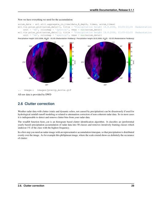
wradlib Documentation, Release 0.1.1 Now we have everything we need for the accumulation: accum_data = wrl.util.aggregate_in_time(data_R_depth, times, accum_times) wrl.vis.polar_plot(accum_data[0], title = ’Precipitation height 18.8.2006, 00:05-01:05 (Radarstation unit = ’mm’, colormap = ’spectral’, vmax = max(accum_data)) wrl.vis.polar_plot(accum_data[1], title = ’Precipitation height 18.8.2006, 01:05-02:05 (Radarstation unit = ’mm’, colormap = ’spectral’, vmax = max(accum_data)) .. image:: images/precip_movie.gif All raw data is provided by DWD 2.6 Clutter correction Weather radar data with clutter (static and dynamic echos, not caused by precipitation) can be disastrously if used for hydrological rainfall-runoff modeling or related to attenuation correction of non-coherent radar data. So in most cases it is indispensable to detect and remove clutter bins from your radar data. The wradlib function histo_cut is an histogram based clutter identification algorithm. It classifies an (preferential yearly based) precipitation accumulation of radar data into 50 classes and removes iteratively framing classes which undercut 1% of the class with the highest frequency. In a first step you need an radar-image with an representative accumulation timespan, so that precipitation is distributed evenly over the image. As for example this philipinean image, where the scale extend shows us definitely the occurance of clutter: 2.6. Clutter correction 29
Page 1: wradlib Documentation Release 0.1.1
Page 4 and 5: 5.3 Users . . . . . . . . . . . . .
Page 6 and 7: wradlib Documentation, Release 0.1.
Page 82 and 83:
wradlib Documentation, Release 0.1.
Page 84 and 85:
Page 86 and 87:
Page 88 and 89:
Page 90 and 91:
Page 92 and 93:
Page 94 and 95:
Page 96 and 97:
Page 98 and 99:
Page 100 and 101:
Page 102 and 103:
Page 104 and 105:
Page 106 and 107:
show all

wradlib Documentation - Bitbucket

Create successful ePaper yourself

Delete template?

Save as template?