wradlib Documentation - Bitbucket

wradlib Documentation, Release 0.1.1
2.1.1 Reading the data
The binary encoding of many radar products is a major obstacle for many potential radar users. Often, decoder software
is not easily available. wradlib support a couple of formats such as the OPERA BUFR and hdf5 implementations,
NetCDF, and some formats used by the Germany Weather Service. We seek to continuously enhance the range of
supported formats.
The basic data type used in wradlib is a multi-dimensional array, the numpy.ndarray. Such an array might e.g. represent
a polar or Cartesian grid, or a series of rain gage observations. Metadata are normally managed as Python dictionaries.
In order to read the content of a data file into a numpy array, you would normally use the wradib.io module. In the
following example, a local PPI from the German Weather Service, a DX file, is read:
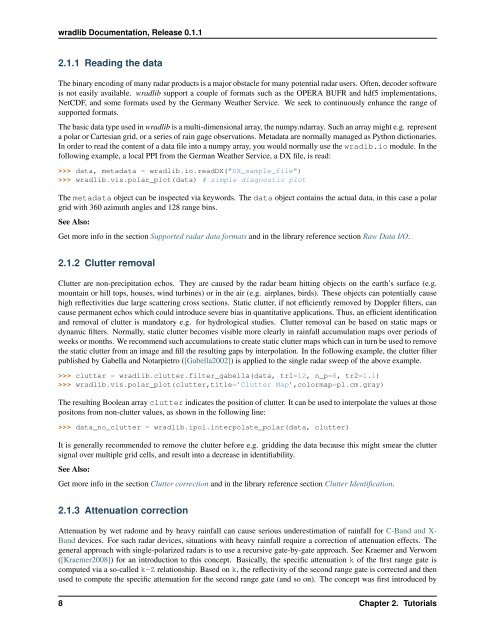
>>> data, metadata = wradlib.io.readDX("DX_sample_file")
>>> wradlib.vis.polar_plot(data) # simple diagnostic plot
The metadata object can be inspected via keywords. The data object contains the actual data, in this case a polar
grid with 360 azimuth angles and 128 range bins.
See Also:
Get more info in the section Supported radar data formats and in the library reference section Raw Data I/O.
2.1.2 Clutter removal
Clutter are non-precipitation echos. They are caused by the radar beam hitting objects on the earth’s surface (e.g.
mountain or hill tops, houses, wind turbines) or in the air (e.g. airplanes, birds). These objects can potentially cause
high reflectivities due large scattering cross sections. Static clutter, if not efficiently removed by Doppler filters, can
cause permanent echos which could introduce severe bias in quantitative applications. Thus, an efficient identification
and removal of clutter is mandatory e.g. for hydrological studies. Clutter removal can be based on static maps or
dynamic filters. Normally, static clutter becomes visible more clearly in rainfall accumulation maps over periods of
weeks or months. We recommend such accumulations to create static clutter maps which can in turn be used to remove
the static clutter from an image and fill the resulting gaps by interpolation. In the following example, the clutter filter
published by Gabella and Notarpietro ([Gabella2002]) is applied to the single radar sweep of the above example.
>>> clutter = wradlib.clutter.filter_gabella(data, tr1=12, n_p=6, tr2=1.1)
>>> wradlib.vis.polar_plot(clutter,title=’Clutter Map’,colormap=pl.cm.gray)
The resulting Boolean array clutter indicates the position of clutter. It can be used to interpolate the values at those
positons from non-clutter values, as shown in the following line:
>>> data_no_clutter = wradlib.ipol.interpolate_polar(data, clutter)
It is generally recommended to remove the clutter before e.g. gridding the data because this might smear the clutter
signal over multiple grid cells, and result into a decrease in identifiability.
See Also:
Get more info in the section Clutter correction and in the library reference section Clutter Identification.
2.1.3 Attenuation correction
Attenuation by wet radome and by heavy rainfall can cause serious underestimation of rainfall for C-Band and X-
Band devices. For such radar devices, situations with heavy rainfall require a correction of attenuation effects. The
general approach with single-polarized radars is to use a recursive gate-by-gate approach. See Kraemer and Verworn
([Kraemer2008]) for an introduction to this concept. Basically, the specific attenuation k of the first range gate is
computed via a so-called k-Z relationship. Based on k, the reflectivity of the second range gate is corrected and then
used to compute the specific attenuation for the second range gate (and so on). The concept was first introduced by
8 Chapter 2. Tutorials