Basic concepts of population genetics - Bioversity International

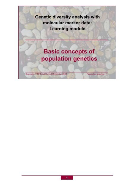
Genetic diversity analysis with
molecular marker data:
Learning module
Basic concepts of
population genetics
Copyright: IPGRI and Cornell University, 2003 Population genetics 1
1

Contents
Definitions
The Hardy-Weinberg principle
Examples of calculating allele frequencies
Reproduction and mating systems
Forces shaping genetic diversity
Appendix 1: Critical values of the chi-square
distribution
Copyright: IPGRI and Cornell University, 2003 Population genetics 2
2

Definitions: Population genetics
The measurement of variability by describing
changes in allele frequency for a particular trait
over time
The analysis of causes leading to those
changes
Copyright: IPGRI and Cornell University, 2003 Population genetics 3
‘Population genetics’ is defined in many ways. In general, we can say that
population genetics is the study of the application of Mendel’s laws and other
genetic principles to entire populations of organisms instead of just to individuals.
Population genetics is also the study of changes in gene frequencies and, as such,
is closely related to evolutionary genetics because evolution depends heavily on
changes in gene frequencies. A short introduction to the main factors possibly
causing changes in genetic diversity may be found in slides 33 to 42 of this section.
Although inspecting all genetic variables present in a population is virtually
impossible, we can examine a population through variation in individual phenotypes
(description of certain morphological or physiological traits) and genotypes
(molecular markers).
3

Phenotype is …
The description of all traits of an individual as
they concern its morphology, physiology,
ecological relationships and behaviour
At any given time, the phenotype is the result of
the genes of the individual interacting with the
environment
Copyright: IPGRI and Cornell University, 2003 Population genetics 4
Phenotypic differences can be either qualitative (present or absent) or can be
quantitative. Qualitative traits can be classified. Quantitative traits are measured.
Individuals share the same phenotype if they look alike. Some genotypes may have
the same phenotype. The distinction between genotype and phenotype is important
in those traits that are influenced by the environment: two individuals with the same
genotype may result in different phenotypes because of the environment.
4

Phenotypic variation
Pink Pale cream Dark pink
Yellow Red
Purple
Light blue
Copyright: IPGRI and Cornell University, 2003 Population genetics 5
5
Dark cream
White
Natural populations are phenotypically diverse. The amount of phenotypic diversity
is extraordinary and obvious, even at the most spontaneous observation.
A population of closely related individuals will show low variability. This is especially
critical if environmental conditions change and that population does not have the
variation to cope with the change. The population could rapidly move towards
extinction.
Population genetics deals with phenotypic diversity, especially where it is due to
differences in the genotypic composition of individuals.

Gene and allele
A gene is the basic physical and functional unit
of heredity, passing information from one
generation to the next
An allele is any of the alternative forms of a
gene that can exist at a single locus
Copyright: IPGRI and Cornell University, 2003 Population genetics 6
Not all of a DNA sequence is made up of genes. Genes are those sections of DNA
that have a known function. They include a transcribed section and a regulatory
element that allows its transcription. The existence of genes is deduced by
observing the segregation of variants in the progeny of crosses, whether naturally or
artificially produced. This observation was the basis on which Gregor Mendel
defined the laws of inheritance at the end of the 19 th century.
Genes may have two or more alleles. Indeed, a gene may have so many alleles as
to constitute an allelic series for that gene. Alleles belonging to a series may show
different patterns of dominance to each other. For example, an allele may show a
dominant effect, which means that it expresses its phenotype, even if accompanied
by a recessive allele. A recessive allele is one where its phenotype is not expressed
in an heterozygous individual. If an allele is codominant, its phenotypic effect will be
intermediate in the heterozygote relative to the effect of an homozygous dominant
and that of an homozygous recessive.
6

Genotype is …
The description of the complete set of genes
that an individual inherits from its parents
The genotype of an individual remains
unchanged throughout its life, regardless of the
environment surrounding and affecting it
Copyright: IPGRI and Cornell University, 2003 Population genetics 7
The term ‘gene’ generally refers to the physical entity that is transmitted from
parents to offspring during the reproductive process that influences hereditary traits.
An individual’s genotype, then, is the sum of all genes inherited from its parents.
Genes determine the composition of proteins and also influence external traits and
behaviour.
7

Genetic variation
Genetic variation deals with the concept of
genotype
Genetic variation affecting traits exists in most
natural populations, but these traits are
influenced by the alleles of many genes in
addition to the effects of the environment
It is difficult to trace phenotypic differences to
the effects of particular genes
Copyright: IPGRI and Cornell University, 2003 Population genetics 8
Hidden genetic variation is even more extensive than that observed through the
phenotype, so much so that it is virtually impossible for two individuals in a
population to have the same genotype at all loci. This genetic variation may be
detected through molecular technologies, which reveal polymorphisms, which are
then useful as genetic markers. However, even molecular tools are limited and,
except for comparisons of entire DNA sequences, most methods are limited to a
certain number of genes or loci. Even so, sufficient variation is usually found in
samples of genes to make assessing the genetic variation possible for most
populations.
As mentioned earlier, because only a small portion of the genome is usually
explored in genetic variation studies, questions arise about the reliability of results
for extrapolation to natural populations. This becomes an important reason to
carefully plan the experiments and pay particular attention to the sampling of both
individuals and the loci to be screened.
8

What is polymorphism?
‘Presence of many forms’
In genetic terms, it refers to the coexistence of
two or more alternative phenotypes in a
population or among populations. In general,
these diverse phenotypes are caused by
alternative alleles of one gene
At the molecular level, polymorphism refers to
the coexistence of alternative banding patterns
or DNA variants when revealed by a given
detection method
Copyright: IPGRI and Cornell University, 2003 Population genetics 9
A gene or a phenotypic trait is said to be polymorphic if more than one form of the
gene or trait exists in a population. Genetic variation, which may cause evolutionary
change, is ever-present.
More information about polymorphism in general, and molecular polymorphism in
particular, is given throughout the training module Using Molecular Marker
Technology in Studies on Plant Genetic Diversity (www.ipgri.cgiar.org/publications).
9

A population is …
Ecologically:
A group of individuals of the same species living within
a restricted geographical area that allows any two
individuals to interbreed
Genetically:
A group of individuals who share a common gene pool
and have the potential to interbreed
Copyright: IPGRI and Cornell University, 2003 Population genetics 10
Populations are extremely complex entities. In population genetics, the focus is on
the local interbreeding unit of a larger population because changes in allele
frequencies occur within such limited units and may result in the evolution of
adaptive traits. These local interbreeding units are usually called local populations,
subpopulations or simply populations. Normally, in a population, members of a
species are unevenly distributed. Subdivision of populations are often due to
accidents in the environment where they are present. In principle, population size is
not infinitely large and does not remain constant.
10

Population structure
Three levels of population structure are identified:
Individual organisms
Subpopulations
Total population
Copyright: IPGRI and Cornell University, 2003 Population genetics 11
A population may be considered as a single unit. However, in many species and
circumstances, populations are subdivided in smaller units. Such subdivision may
be the result of ecological (habitats are not continuous) or behavioural factors
(conscious or unconscious relocation). If a population is subdivided, the genetic
links among its parts may differ, depending on the real degree of gene flow taking
place.
A population is considered structured if (1) genetic drift is occurring in some of its
subpopulations, (2) migration does not happen uniformly throughout the population,
or (3) mating is not random throughout the population. A population’s structure
affects the extent of genetic variation and its patterns of distribution.
See the following slides and the Glossary for more details on these new concepts
(e.g. gene flow, migration).
11

Gene flow
Pollinating insects
carry pollen grains from
population Y (allele a >
allele A) to population X
Population X
p = 0.80 (frequency of allele A)
q = 0.20 (frequency of allele a)
Copyright: IPGRI and Cornell University, 2003 Population genetics 12
12
a
a
A
a a
A a
a
Migrant population Y
p = 0.10 (frequency of allele A)
q = 0.90 (frequency of allele a)
Gene flow is the passage and establishment of genes typical of one population in
the genepool of another by natural or artificial hybridization and backcrossing.
In the drawing above, population Y has a higher frequency of allele a (q = 0.90).
Pollinators flying from that population will transport more copies of allele a when
they move towards another population X. The resulting effect of gene flow is
observed in subsequent generations of population X as an increase in the frequency
of the migrant allele a.

Allele frequency
Allele frequency is the concept used to quantify
genetic variation
It is defined as a measure of the commonness
of a given allele in a population, that is, the
proportion of all alleles of that gene in the
population that are specifically this type
Copyright: IPGRI and Cornell University, 2003 Population genetics 13
An allele is an alternative form of a gene. If a gene corresponds to a specific
sequence of nucleotides along a DNA molecule, the alleles represent the different
sequences of nucleotides that are possible for that particular locus.
Often the term ‘gene’ is used synonymously with ‘allele’ and, hence, ‘gene
frequency’ is sometimes used synonymously with ‘allele frequency’. Allelic
differences at a single locus in a population indicate genetic variation. This genetic
variation needs to be quantified for different genes and for different individuals or
populations.
13

Calculating the allele frequency
P(A) = [2(AA) + (Aa)]/2n
Twice the number of homozygous genotypes
with that allele (because homozygotes carry two
copies each of the same allele),
plus the number of heterozygous genotypes
with that allele (because heterozygotes carry
only one copy of a particular allele),
divided by two times the total number of
individuals in the sample (because each
individual carries two alleles per locus)
Copyright: IPGRI and Cornell University, 2003 Population genetics 14
Note that any result obtained with this formula will only be an estimate of the total
allele frequency in the population, because only a sample of individuals is usually
studied. However, if the sampling of individuals is well done, that is, the size of the
sample is sufficiently large, then it can be assumed that our calculation is close to
the true allele frequency. As a rule of thumb, allele frequency estimates should be
performed, where possible, on samples of 100 individuals or more.
14

Genotype frequency
This is the frequency of a given genotype in a
population
The frequencies of various types of breeding
systems determine the mathematical
relationship between the allele and genotype
frequencies
Copyright: IPGRI and Cornell University, 2003 Population genetics 15
The natural breeding system of individuals can be examined through studies of the
frequencies with which alternative genotypes occur in a population. When a
population undergoes mating that is random relative to the alleles of interest, certain
patterns of genotype frequencies may be expected.
Genotype frequencies are also used to estimate the amount of self-pollination
occurring in populations of individuals that have this or mixed type of reproduction.
The mating or breeding system, therefore, has a significant effect on the frequency
of occurrence of alternative genotypes in a given population.
15

The Hardy-Weinberg principle
A population with random mating results in an
equilibrium distribution of genotypes after only
one generation, so that the genetic variation is
maintained
When the assumptions are met, the frequency
of a genotype is equal to the product of the
allele frequencies
AA Aa aa
p 2 2pq q 2
Copyright: IPGRI and Cornell University, 2003 Population genetics 16
The H-W equilibrium states that sexual reproduction does not reduce genetic
variation generation after generation; on the contrary, the amount of variation
remains constant if there are no disturbing forces acting against it. It establishes the
relationship for calculating genotype frequencies under random mating and, in doing
so, provides the foundation for many studies in population genetics.
This principle describes the expectations for allele frequencies in an idealized
situation where,
The organism is diploid
Reproduction is sexual
Generations are not overlapping
Mating is random
Population size is very large
Migration is negligible
Mutations can be ignored
Natural selection does not affect the alleles under consideration
Note that most crop plants violate at least one of these assumptions!
16

Demonstrating the H-W principle
Genotype
frequencies
Generation 0
N
A 1 A 1 , A 1 A 2 , A 2 A 2
p 2 , 2pq, q 2
Genotype frequencies
do not change from
generation to generation
Generation 1
N
A 1
A 1
A 1 A 1 , A 1 A 2 , A 2 A 2
p 2 , 2pq, q 2
gametes
gametes
Copyright: IPGRI and Cornell University, 2003 Population genetics 17
17
A 2
A 2
Random mating
A 1
(p)
A 2
(q)
A 1
(p) (q)
A 1 A 1 (p 2 ) A 1 A 2 (pq)
A 1 A 2 (pq)
Zygotes
A 2
A 2 A 2 (q 2 )
The starting point is generation 0. We have a gene with two alleles, A 1 and A 2 . The
frequency of allele A 1 is p and the frequency of allele A 2 is q. The genotype
frequencies in generation 0 are for A 1 A 1 = p 2 ,for A 1 A 2 = 2pq and for A 2 A 2 = q 2 . If
random mating occurs, the probability of any allele from the female plant meeting
any allele from the male plant will be the same. The table to the right of the slide
depicts the four possible genotypes for next generation. The frequency of
occurrence of each genotype is given by the product of the frequency of each allele
in the genotype (e.g. for A 1 A 1 is p x p = p 2 ). If the results in the table are
summarized, as in the blue inset at the bottom of the slide, we see that the
genotype frequencies in generation 1 remain the same as in the previous
generation.

An example of three populations in Hardy-
Weinberg equilibrium
Popul.
Pop. 1
Pop. 2
Pop. 3
Genotypes of G 0
A 1 A 1
0.6
0.49
0.4
A 1 A 2
0.2
0.42
0.6
A 2 A 2
0.2
0.09
0.0
p
0.7
0.7
0.7
Frequencies
G 0
0.3
0.3
0.3
Copyright: IPGRI and Cornell University, 2003 Population genetics 18
q
18
Genotypes of G 1
A 1 A 1
0.49
0.49
0.49
A 1 A 2
0.42
0.42
0.42
A 2 A 2
Population genotype frequencies are given in rows. Generations (G 0 and G 1 ) are
given in columns. Again, we have one gene with two alleles, A 1 and A 2 . The
frequency of allele A 1 is p and the frequency of allele A 2 is q. Genotype frequencies
are different for each population in generation 0 (e.g. the frequency of A 1 A 1 in
population 1 is 0.6; in population 2, 0.49; and in population 3, 0.4, and so on for the
other genotypes). We note, though, that the allele frequencies in the three
populations are similar in G 0 (p = 0.7 and q = 0.3). In the next generation, G 1 , if all
requirements of the H-W principle are met, the genotype frequencies in the three
populations balance (now the frequency of A 1 A 1 is 0.49 in the three populations,
and the same happens with the frequencies of A 1 A 2 and A 2 A 2 ). The allele
frequencies are kept.
0.09
0.09
0.09
p
0.7
0.7
0.7
G 1
q
0.3
0.3
0.3

The chi-square test
This hypothesis test is useful for determining
whether the allelic frequencies are in H-W
equilibrium
The procedure is as follows:
Define H 0 (and H a )
Define significance level
Perform the statistical test
Apply the decision criteria
Copyright: IPGRI and Cornell University, 2003 Population genetics 19
H 0 = the hypothesis that says the allele frequencies for trait Q in a given population are in H-
W equilibrium.
H a = an alternative hypothesis that says the allele frequencies for trait Q are not in H-W
equilibrium.
We choose a significance level to give us a certain percentage of confidence in our results.
The statistical test follows the formula:
Where,
ST = statistical test k = number of genotypic classes
O = observed frequencies m = number of alleles
E = expected frequencies df = degrees of freedom
If our sample allows for only 1 degree of freedom, then the difference in frequencies
is reduced by 0.5, a correction factor, such as:
The decision criteria is applied as follows:
Where,
If 2 cal 2 tab then H0 is accepted; and, if 2 cal > 2 tab then H0 is rejected
cal = the result of calculating ST with the data obtained in our sample
tab = the value identified in the table (a 2 table may be found in Appendix
1, click here).
19
Oi Ei
(Ei)
2
2
ST k mdf
2
Oi Ei
0.5
Ei

Applying the 2 test: An example
Genotype AA Aa aa
No. observed 169 520 311
No. expected 250 500 250
X 2 calculation (169-250-0.5) 2 /250 (520-500-0.5) 2 /500 (311-250-0.5) 2 /250
X 2 value +25.921 +0.760 +14.641 41.322
= 0.05
Copyright: IPGRI and Cornell University, 2003 Population genetics 20
20
Decision criteria:
2 cal (41.322) > 2 tab (3.8)
H 0 is rejected
In this example, let’s say that allele frequencies were 0.429 for A 1 and 0.571 for A 2 .
Each genotypic class was represented as in the table on the slide above.
The hypotheses being tested are:
H 0 = this population is in H-W equilibrium for its allele frequencies
H a = this population is not in H-W equilibrium for its allele frequencies
Because the number of genotypic classes is 3 and we therefore have only
1 degree of freedom, we apply the correction factor in our calculation of the 2
elements.
The 2 calculated is 41.322. With this figure and with an error margin of 0.05%, the
statistical evidence rejects H 0 , which means that this population is not in H-W
equilibrium for the trait under study.

Calculating allele frequencies: Examples
Calculating allele frequencies with a codominant
marker
Calculating allele frequencies with a dominant
marker
Calculating the allele frequencies with a
codominant gene having multiple alleles
Copyright: IPGRI and Cornell University, 2003 Population genetics 21
In the next few slides we show examples of calculations of allele frequencies for
results obtained with different marker types. The examples are given with figures
that emulate real gels and the bands obtained through the application of molecular
markers. For details on molecular marker technologies and the interpretation of
bands, see the training module Using Molecular Marker Technology in Studies on
Plant Genetic Diversity (http://www.ipgri.cgiar.org/publications/pubfile.asp?ID_PUB=912).
21

… with a codominant marker
Locus A
Gel
Indiv. 1 Indiv. 2 Indiv. 3
A1 1 1 0
A2 0 1 1
M
Genotypes
A 1A 1
Individuals
1 2 3
Scoring bands
Copyright: IPGRI and Cornell University, 2003 Population genetics 22
22
A 1A 2
Locus A
A 2A 2
M 1 2 3
1,0 1,1 0,1
(continued on next slide)
With a codominant marker, the genotypes of the three genotypic classes can be
observed for the two homozygotes and the heterozygote. In the drawing above, top
centre, we see a gel image with the banding pattern of a codominant marker for a
single locus of a diploid organism. We need to score the bands in the gel and
convert them to numbers. To do so, each of the band sizes (the band in the same
row) is scored and transformed to a 1 if it is present or to a 0 if it is absent. We can
do it by band, as in the table at the bottom left, or by genotype, as at the bottom
right corner. In the table below we can see the calculations of the expected and
observed genotype frequencies, as well as the allele frequencies. (M = size
marker.)
Genotypes
Genotype frequency
(expected)
Number of
individuals
Genotype frequency
(observed)
A 1 A 1
p 2
n 11 = 40
P 11 = n 11 /n
= 0.20
A 1 A 2
2pq
n 12 = 20
P 12 = n 12 /n
= 0.10
A 2 A 2
q 2
n 22 = 140
P 22 = n 22 /n
= 0.70
p = (2n 11 /2n) + (n 12 /2n) = P 11 + ½ P 12 = 0.20 + ½ (0.10) = 0.25
q = (2n 22 /2n) + (n 12 /2n) = P 22 + ½ P 12 = 0.70 + ½ (0.10) = 0.75
Total
1
n = 200
1

Locus
A
B
D
… with a codominant marker (continued)
Locus A
Locus B
Locus D
Locus A
Locus B
Locus D
Individuals
M 1 2 3 4 5 6 7 8 9 10
M
1 2 3 4 5 6 7 8 9 10
1,1 1,0 1,1 0,1 0,1 1,1 1,0 0,1 0,1 0,1
1,0 1,0 1,0 1,1 0,1 1,0 1,0 1,0 1,0 1,0
1,0 1,0 1,1 0,1 0,1 1,1 0,1 0,1 1,1 1,1
Copyright: IPGRI and Cornell University, 2003 Population genetics 23
The example in this slide is similar to that in the previous slide, but with 10 individuals and
three segregating loci (A, B and D). For ease of presentation, only one scoring method is
used (bottom of slide). (M = size marker.)
Note that a gel, like the one in the example, can be obtained only by multiplexing, that is,
loading different marker reactions into the same well.
Below, we see a table with the calculations of genotype and allele frequencies. (exp. =
expected values; obs. = observed values.)
Genotypes
23
Allele freq.
Genotype freq. (exp.) 2pq
1 p q
Number of indivs.
Genotype freq. (obs.)
Genotypes
Genotype freq. (exp.)
Number of indivs.
Genotype freq. (obs.)
Genotypes
Genotype freq. (exp.)
Number of indivs.
Genotype freq. (obs.)
Data analysis
A 1 A 1
p 2
2
P 11 = 0.2
B 1 B 1
p 2
8
P 11 = 0.8
D 1 D 1
p 2
2
P 11 = 0.2
A 1 A 2
3
P 12 = 0.3
B 1 B 2
2pq
1
P 12 = 0.1
D 1 D 2
2pq
4
P 12 = 0.4
A 2 A 2
q 2
5
P 22 = 0.5
B 2 B 2
q 2
1
P 22 = 0.1
D 2 D 2
q 2
4
P 22 = 0.4
Total
10
1
Total
1
10
1
Total
1
10
1
0.35
p
0.85
p
0.40
0.65
q
0.15
q
0.60

… with a dominant marker
Locus A
Gel
M
Genotypes
Individuals
1 2
AA, A a
a a
Copyright: IPGRI and Cornell University, 2003 Population genetics 24
24
Locus A
Scoring bands
M 1 2
1 0
(continued on next slide)
With a dominant marker, only two genotypic classes can be observed: AA + Aa and
aa, that is, one of the homozygote classes is confounded with the heterozygote. The
gel image with the banding pattern of a dominant marker for a single locus will show
either one band or no band for each individual. The bands are scored in a way
similar to that for the codominant marker, where bands are converted to a score of 1
if present or 0 if not. (M = size marker.)
The calculations of frequencies are performed as shown in the table below.
(p, q = allele frequencies.)
Phenotypes
Genotypes
Phenotype frequencies
(expected)
Number of individuals
Phenotype frequencies
(observed)
AA
A _
p 2 + 2pq
n 1 = 84
P 1 = n 1 /n = 0.84
q = (n 2 /n) = (P 2 )= (0.16 ) = 0.4
p = (1 – q ) = 0.6
Aa
aa
aa
q 2
n 2 = 16
P 2 = n 2 /n = 0.16
Total
1
n = 100
This is a biased estimate
because it does not take into
account the recessive
alleles in the heterozygotes.
1

Locus A
Locus B
Locus D
… with a dominant marker (continued)
Locus A
Locus B
Locus D
M 1 2 3 4 5 6 7 8 9 10
M 1 2 3 4 5 6 7 8 9 10
1 0 1 1 0 1 1 1 1 1
0 1 0 0 0 1 0 0 1 0
1 1 1 1 0 1 1 0 1 1
Copyright: IPGRI and Cornell University, 2003 Population genetics 25
25
Individuals
Here we have an example similar to that in the previous slide but with 10 individuals and three
segregating loci (A, B, and D). (M = size marker.)
Non-segregating bands (monomorphic) are not scored and thus are not included in the analysis.
Below, we see the table with calculations of genotype and allele frequencies:
Locus
s
A
B
D
Genotypes
Genotype freq. (exp.)
Number of indivs.
Genotype freq. (obs.)
Genotypes
Genotype freq. (exp.)
Number of indivs.
Genotype freq. (obs.)
Genotypes
Number of indivs.
Genotype freq. (obs.)
Data analysis
A 1 _
p 2 + 2pq
8
P 1 = 0.8
B 1 _
p 2 + 2pq
3
P 1 = 0.3
D 1 _
8
P 1 = 0.8
A 2 A 2
B 2 B 2
D 2 D 2
2
P 2 = 0.2
Total
Total
10
1
Allele freq.
0.55
0.16
q 1
2
p2 Genotype freq. (exp.) + 2pq
p q
q 2
2
P 2 = 0.2
q 2
7
P 2 = 0.7
Total
1
10
1
1
10
1
p
p
0.55
We cannot distinguish heterozygotes, but we can estimate the expected number of
heterozygotes in a population. For example, if sample size = 1000, then:
For locus A, no. expected heterozygotes = 2pqN = 2(0.55)(0.45)(1000) = 495
For locus B, no. expected heterozygotes = 2pqN = 2(0.16)(0.84)(1000) = 269
and so on ...
q
0.45
q
0.84
0.45

... with a codominant gene having multiple
alleles
Genotypes
Genotype frequencies
(expected)
Number of individuals
Genotype frequencies
(observed)
A 1 A 1
p 1 2
n 11
P 11 =
n 11 /n
A 1 A 2
2p 1 p 2
n 12
P 12 =
n 12 /n
p 1 = P 11 + ½ i 1 P 1j
p 3 = P 33 + ½ j 3 P 3j
A 1 A 3
2p 1 p 3
n 13
P 13 =
n 13 /n
p n = P nn + ½ j n P nj
Copyright: IPGRI and Cornell University, 2003 Population genetics 26
26
A 2 A 2
p 2 2
n 22
P 22 =
n 22 /n
A 2 A 3
2p 2 p 3
n 23
P 23 =
n 23 /n
p 2 = P 22 + ½ j 2 P 2j
p 4 = P 44 + ½ j 4 P 4j
...
...
...
...
A n A n
p n 2
n nn
P nn =
n nn /n
Total
(continued on next slide)
This is the situation encountered when markers such as microsatellites are used.
We have a locus A with n alleles A 1 , A 2 , A 3 , ..., A n and allele frequencies p 1 , p 2 , p 3 ,
..., p n , respectively, such that A 1 = A 2 = A 3 = ... = A n
1
n
1

... with a codominant gene having multiple
alleles (continued)
Locus A
Gel
Ind.1 Ind.2 Ind.3 Ind.4 Ind.5 Ind.6
A1 1 1 1 0 0 0
A2 0 1 0 1 1 0
A3 0 0 1 0 1 1
M
Genotypes
A 1 A 1
Individuals
1 2 3 4 5 6
A 1A 2
A 1 A 3
Scoring bands
Copyright: IPGRI and Cornell University, 2003 Population genetics 27
27
A 2A 2
Locus A
A 2 A 3
A 3A 3
M 1 2 3 4 5 6
(1,0,0) (1,1,0) (1,0,1) (0,1,0) (0,1,1) (0,0,1)
Again, with a codominant marker, the genotypes of the three genotypic classes can
be observed. In the drawing above, top centre, we see a gel image with the banding
pattern of a codominant marker with three alleles (A 1 , A 2 and A 3 ) in a diploid
sample. We score each band (each row) independently, and transform them to a
score of 1 if present or a score of 0 if not. We can do it by band (bottom left of slide)
or by genotype (bottom right corner). In the table below, we can see the calculations
of the expected and observed genotype frequencies, as well as the allele
frequencies (p 1 , p 2 and p 3 ). (M = size marker.)
Genotypes
Genotype
frequency
(exp.)
Number of
individuals
Genotype
frequency
(obs.)
A 1 A 1
p 1 2
n 11 =
4
P 11 =
n 11 /n
= 0.17
A 1 A 2
2p 1 p 2
n 12 =
6
P 12 =
n 12 /n
= 0.25
A 1 A 3
2p 1 p 3
n 13 =
0
P 13 =
n 13 /n
= 0
A 2 A 2
p 2 2
n 22 =
10
P 22 =
n 22 /n =
0.42
A 2 A 3
2p 2 p 3
n 23 =
2
P 23 =
n 23 /n
= 0.08
A 3 A 3
p 3 2
n 33 =
2
P 33 =
n 33 /n
= 0.08
p 1 = P 11 + ½P 12 + ½P 13 = P 11 + ½ j 1 P 1j = 0.17 + ½(0.25 + 0.00) = 0.30
p 2 = P 22 + ½P 21 + ½P 23 = P 22 + ½ j 2 P 2j = 0.42 + ½(0.25 + 0.08) = 0.59
p 3 = P 33 + ½P 31 + ½P 32 = P 33 + ½ j 3 P 3j = 0.08 + ½(0.00 + 0.08) = 0.12
Total
1
n = 24
1

Reproduction and mating systems
Outbreeding, inbreeding or asexual
reproduction
They influence:
The degree of genetic relatedness among mates
The organization of genes into genotypes
Copyright: IPGRI and Cornell University, 2003 Population genetics 28
In principle, outbreeding occurs as random mating, and inbreeding and asexual
reproduction both involve nonrandom mating.
Outcrossing species, compared with inbreeders, may retain large numbers of
deleterious recessives because the dominance situation hides them. The
recessives undergo frequent recombination, resulting in new gametic types.
Dominance refers to situations where, under heterozygous conditions, one allele
has a phenotypic effect that is strong enough to conceal the presence of the other
(recessive) allele. In a situation of dominance, only two phenotypes can be
observed: the dominant phenotype that is a mixture of the homozygous dominant
and the heterozygous, and the recessive phenotype.
In cross-pollinating species, selfing leads to inbreeding depression because it
increases the proportion of homozygotes, thus permitting rare recessive alleles to
become visible. Heterozygotes in cross-pollinating species have a more favourable
effect.
In organisms with asexual reproduction, a variety of consequences result,
depending on its type. Although asexual reproduction may be a constant mode of
reproduction, it may be combined with cycles of sexual reproduction, which allow
recombination of the current variation and, as such, the generation of new forms or
combinations. If only asexual reproduction occurs in the population, genotypic
frequencies cannot be changed.
28

Random mating
Mating that takes place at random, that is, the
chances of individual A mating with individual B
do not depend on the genotypes of either
If random mating occurs, the chance that an
individual mates with a given genotype is equal
to the frequency of that genotype in the
population
Copyright: IPGRI and Cornell University, 2003 Population genetics 29
Random mating is typically found in many outbreeding populations. For example,
we may have a population in which genotype AA is present 10% of times, Aa 58%
of times and aa 32% of times. If mating is random, then the chances of an individual
AA mating with another AA is 10/100, Aa 58/100, or aa 32/100.
29

Nonrandom mating
Classified mating:
Positive: mating among
individuals with similar
phenotypes
Inbreeding:
Negative: mating among individuals
with dissimilar phenotypes
Mating among relatives
Copyright: IPGRI and Cornell University, 2003 Population genetics 30
30
X X
X
Parents
Full sibs
Inbred individual
Nonrandom mating occurs when individuals that are more closely (inbreeding) or
less closely related mate more often than would be expected by chance for the
population.
Self-pollination or inbreeding is similar to mating between relatives. It increases the
homozygosity of a population and its effect is generalized for all alleles. Inbreeding
per se does not change the allelic frequencies but, over time, it leads to
homozygosity by slowly increasing the two homozygous classes.

Inbreeding coefficient
It compares the actual proportion of
heterozygous genotypes with those expected
under random mating
F
H0H F is the inbreeding coefficient and measures the
reduction of heterozygosity
Copyright: IPGRI and Cornell University, 2003 Population genetics 31
31
H
H = actual frequency of heterozygotes in the population.
H 0 = expected number of heterozygotes under random mating.
The inbreeding coefficient indicates the degree of inbreeding in a population.
0

What happens in selfing?
100.0
75.5
50.0
25.5
%
0.0
0 1 2 3 4 5 6 7 8
Generations
Copyright: IPGRI and Cornell University, 2003 Population genetics 32
Generation
G 0
G 1
G 2
G 3
G 4
G 5
G 6
G 7
G 8
32
Heterozygosity
Homozygosity
Selfing is a powerful inbreeding system that allows the attainment of high
levels of homozygosity within few generations. Simultaneously,
heterozygosity decreases. The chart on the slide shows the phenomenon
and, in the table below, we can see the changing values of homozygosity
and heterozygosity in
9 generations (G 0 to G 8 ).
Selfed genotypes
ratio/generation
Aa
1AA, 2Aa, 1aa
6AA, 4Aa, 6aa
28AA, 8Aa, 28aa
120AA, 16Aa, 120aa
496AA, 32Aa, 496aa
2016AA, 64Aa, 2016aa
8128AA, 128Aa, 8128aa
32640AA, 256Aa,
32640aa
Homozygosit
y (%)
0
50
75
87.5
93.75
96.875
98.4375
99.21875
99.60938
Heterozygosit
y (%)
100
50
25
12.5
6.25
3.125
1.5625
0.78125
0.390625

Forces shaping genetic diversity
Mutation
Migration
Recombination
Selection
Drift
Copyright: IPGRI and Cornell University, 2003 Population genetics 33
If, for any reason, a population becomes homogeneous, evolution would not occur.
Thus, constant change essentially depends on new variation.
A genetic population is the aggregate of allelic frequencies of all genes in that
population. Populations change or evolve because their gene frequencies
experience change. Several factors can produce changes in fitness—the capability
of an individual to survive until reproduction is achieved. If the fitness of an
individual in a population changes, the genotypes in the subsequent generation will
not be directly related to the gene frequencies of the former population, thus driving
the population to evolve.
Because changes in populations require changes in gene frequencies, we must
understand how these frequencies can change. In the next slides, we discuss the
primary causes of change: mutation, migration, recombination, selection and drift.
33

Mutation
It is the ultimate source of variation and may be
caused by:
Errors in DNA replication
Damage by radiation
Mutation increases diversity but, because
spontaneous mutations are rare, the rate of
change in gene frequency is very low
Consequently, mutation alone does not drive
the evolution of populations and species
Copyright: IPGRI and Cornell University, 2003 Population genetics 34
The simplest mutation is that which produces a change in a single nucleotide in the
DNA sequence of a gene. A mutation can cause one allele to change to another
allele already present in the population (from a dominant to a recessive) or it could
create a completely new allele. Mutations may be adverse or favourable. Many will
be adverse and disappear. But, if they are good for the individual, then frequencies
of that allele will increase from generation to generation. Moreover, this mutation
may migrate to other populations and spread.
Note: Genomes may go through a process known as gene duplication. This event
helps the individual to endure an unfavourable mutation in a copy of the gene
without major difficulties, because the other copy of the gene still may function
appropriately. More changes may affect the mutated gene and determine different
types of adaptation for the individual.
34

Migration
It is the movement of individuals or any form of
introduction of genes from one population to
another
Migration increases diversity and its rate can be
large, causing significant changes in frequency
The change in gene frequency is proportional to
the difference in frequency between the
recipient population and the average of the
donor populations
Copyright: IPGRI and Cornell University, 2003 Population genetics 35
From a genetic perspective, migration implies not only the movement of individuals
into new populations but that this movement introduces new alleles into the
population (gene flow). Changes in gene frequencies will occur through migration
either because more copies of an allele already present will be brought in or
because a new allele arrives.
Several factors affect migration in crop species:
Breeding system
Sympatry with wild and/or weedy relatives
Pollinators
Seed dispersal
The immediate effect of migration is to increase a population’s genetic variability
and, as such, helps increase the possibilities of that population to withstand
environmental changes. Migration also helps blend populations and prevent their
divergence.
35

Recombination
It is the process whereby a cell generates new
chromosomal combinations, compared with that
cell or with those of its progenitors
It does not create new diversity but generates
new combinations of the existing diversity
Genetic variance through recombination, given
that segregating alleles exist at different loci,
can occur very quickly
Copyright: IPGRI and Cornell University, 2003 Population genetics 36
Genetic diversity through recombination is the result of reshuffling the genetic
components of the original type. Mechanisms exist to generate allelic diversity
(intragenic recombination) and genomic diversity (new multigene combinations).
36

Selection
It is the inherited ability of organisms to survive and
reproduce. It acts in such a manner that, with time,
superior genotypes increase their frequency in the
population
Copyright: IPGRI and Cornell University, 2003 Population genetics 37
As a result of mutation, new forms develop. These forms, as explained, may be
favourable or deleterious to the individual’s ability to survive. If changes are
advantageous, then the new alleles will tend to prevail by being selected in the
population.
The effect of selection on diversity may be:
Directional, where it decreases diversity
Balancing, where it increases diversity. Heterozygotes have the highest
fitness, so selection favours the maintenance of multiple alleles
Frequency dependent, where it increases diversity. Fitness is a function of
allele or genotype frequency and changes over time
37

Drift
A a
Zygotes
A a A a A a
A A A A a a a a
A a
A A A a A A
A A A A a a a a
a a a a
A A a a a a a a
a a a a
A a A A
a a a a
Genepool Gametic sampling
Copyright: IPGRI and Cornell University, 2003 Population genetics 38
38
a
a
a
a
a
a
a
a
A
A
a
A
a
a
A
a
A
A
A A a A A
a
a
a
a
A
A A a a A
a
A a A
a
a
a
a
A
a
a
a
a a a a a
a
a
a
a
a
a
a
a
a
a
a
a
a
a
G 0
p = 0.5
q = 0.5
G1 p = 0.625
q = 0.375
G2 p = 0.3125
q = 0.6875
G3 p = 0.0
q = 1.0
Genetic drift refers to fluctuations in allele frequencies that occur by chance
(particularly in small populations) as a result of random sampling among gametes.
Drift decreases diversity within a population because it tends to cause the loss of
rare alleles, reducing the overall number of alleles.
In the example above, population size is constant in each generation (8 individuals).
Each individual may produce thousands of gametes but, from the total genepool in
each generation, only 2N gametes per individual are needed (16 in our example).
This situation is similar to extracting small samples from two boxes, one containing
a million white balls and the other a million red balls. In each extracting experiment,
we may take a different number of white and red balls. We simulate that, in
generation G 0 , 10 gametes of the thousands possible carried allele A and only 6
carried allele a. In G 1 , from those gametes that participated in the constitution of the
zygotes for next generation, 5 carried allele A and 11 allele a, and so on. These
values vary randomly. In G 3 all individuals are formed by allele a (homozygotes)
and allele A is lost.

Effective population size
Ne is the number of parents responsible for the
genetic composition of the next generation
Ne is generally less than N because of
Variation of population size from generation to
generation
Unequal sex ratio
Overlapping generations
Geographic dispersion of populations
Copyright: IPGRI and Cornell University, 2003 Population genetics 39
How big is the population?
The actual number of individuals in a population is called the census number
(N). This number is often an imprecise representation of the population size
from a genetic standpoint.
The effective population size (Ne) describes the size of an ideal population
that shows the same rate of loss of genetic variation due to genetic drift as for
the population of interest.
39

Consequences of a decreasing population
size
Genetic drift, with random variation of allele
frequencies
Inbreeding
Homozygosity: fixation and loss of alleles
Subpopulation differentiation
AA
aa
AA
AA AA
aa aa
aa
AA Aa AA
Aa Aa
aa
aa Aa
AA aa
aa Aa
Aa Aa
AA AA
aa Aa Aa
Aa
Aa
Population size
is reduced
AA
AA
aa
AA
Aa
AA
Aa
Mating among
relatives
aa AA
Copyright: IPGRI and Cornell University, 2003 Population genetics 40
Events that reduce population size:
Domestication
40
aa
aa
aa
aa
AA
aa
aa
Aa
AA
AA
Aa AA
AA AA
aa
Homozygosity
increased
Subpopulations (inbreeding, clonal reproduction)
Long-range dispersal (founder effect)
Regeneration of genetic resources collections
aa
aa
aa aa
aa
aa
aa
aa aa
AA
AA
AA
AA
AA
AA
AA
AA
AA
Population
differentiation
Fixation
(continued on next slide)

Consequences … (continued)
A bottleneck develops when the population size
drops sharply
The founder effect occurs when a few
individuals colonize and become established in
a new environment
p = 0.5 (frequency of A 1 )
q = 0.5 (frequency of A 2 )
N
A1A1 A1A1 A1A2 A1A1 A1A1 A1A2 A1A1 A2A2 A2A2 A2A2 A2A2 A1A2 A2A2 A1A1 A2A2 A2A2 A1A2 A1A1 A1A2 A1A2 A1A1 A1A2 A1A2 A2A2 A 2 A 2
Bottleneck
Copyright: IPGRI and Cornell University, 2003 Population genetics 41
41
A 2 A 2
p = 0.0 (frequency of A 1 )
q = 1.0 (frequency of A 2 )
A2A2 A2A2 A2A2 A2A2 A2A2 A2A2 A2A2 A2A2 A2A2 A2A2 A2A2 A2A2 A2A2 A2A2 A2A2 A2A2 Small populations are highly vulnerable to extinction because the surviving sample
may not be representative of the pre-crash genepool.
Both effects depend on the number of survivors (or colonizers) and the rate of
population growth.
The graphic in the slide shows a bottleneck effect. To the left is a population in
Hardy-Weinberg equilibrium with allele frequencies of 0.5. If a sudden reduction
occurs, then the original size restored, the result may be a loss of alleles and the
fixation of others. In the example (right), only A 2 A 2 survived and allele A 1 was lost.
time

With bottleneck and founder effects …
Heterozygosity declines at the rate of:
H 1 = (1 – 1/2N)H 0
Alleles are lost at the rate of:
P = p 2N + q 2N
Copyright: IPGRI and Cornell University, 2003 Population genetics 42
Heterozygosity decline
Where,
Then:
Allele loss
Where,
Then:
H 1 = final heterozygosity
H 0 = initial heterozygosity
N = population size
If N = 100 and H 0 = 0.25, then H 1 = 0.24875
If N = 40 and H 0 = 0.25, then H 1 = 0.24685
P = allele loss
p and q = allele frequencies
2N = total number of alleles in the population
If N = 100, p = 0.90 and q = 0.1, then P = 7.05508 x 10 -10
If N = 15, p = 0.90 and q = 0.1, then P = 0.0423911
If N = 10, p = 0.90 and q = 0.1, then P = 0.12157665
42

Appendix 1
Copyright: IPGRI and Cornell University, 2003 Population genetics 43
Appendix 1. Critical values of the chi-square distribution
43

In summary
To analyse and interpret genetic diversity data we
must be acquainted with:
A few basic definitions of population genetics
The Hardy-Weinberg principle
Calculating allele and genotype frequencies
The primary causes of changes in genetic diversity:
mutation, migration, recombination, selection and drift
Copyright: IPGRI and Cornell University, 2003 Population genetics 44
44

By now you should know …
The basic definitions used in population genetics
The Hardy-Weinberg principle
How to calculate allele frequencies with marker
data
The mating system’s effect on a population’s
diversity
The main sources of variation and their
consequences
Copyright: IPGRI and Cornell University, 2003 Population genetics 45
45

If you would like to read more …
Copyright: IPGRI and Cornell University, 2003 Population genetics 46
de Vicente, M.C. and T. Fulton. 2003. Using Molecular Marker Technology in
Studies on Plant Genetic Diversity.
Doolittle, D.P. 1987. Population Genetics: Basic Principles. Springer-Verlag, Berlin.
Falconer, D.S. and T.F.C. Mackay (eds.). 1996. Introduction to quantitative genetics
(4th edn.). Longman Group, London.
Griffiths, A.J.F., J.H. Miller, D.T. Suzuki, R.C. Lewontin and W.M. Gelbart (eds.).
1996. An Introduction to Genetic Analysis (6th edn.). Freeman and Co., NY.
Hartl, D.L. 1988. A Primer of Population Genetics (2nd edn.). Sinauer Associates,
Sunderland, MA.
Hedrick, P.W. 1985. Genetics of Populations. Jones and Barlett Publishers, Boston,
MA.
Snedecor, G.W. and W.S. Cochran (eds.). 1980. Statistical Methods (7th edn.).
Iowa State University Press, Ames, IO.
46

Next
Measures of genetic diversity
Software programs for analysing genetic
diversity
Glossary
Copyright: IPGRI and Cornell University, 2003 Population genetics 47
47