Basic concepts of population genetics - Bioversity International
Basic concepts of population genetics - Bioversity International
Basic concepts of population genetics - Bioversity International

You also want an ePaper? Increase the reach of your titles
YUMPU automatically turns print PDFs into web optimized ePapers that Google loves.
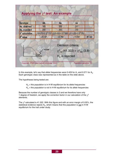
Applying the 2 test: An example<br />
Genotype AA Aa aa<br />
No. observed 169 520 311<br />
No. expected 250 500 250<br />
X 2 calculation (169-250-0.5) 2 /250 (520-500-0.5) 2 /500 (311-250-0.5) 2 /250<br />
X 2 value +25.921 +0.760 +14.641 41.322<br />
= 0.05<br />
Copyright: IPGRI and Cornell University, 2003 Population <strong>genetics</strong> 20<br />
20<br />
Decision criteria:<br />
2 cal (41.322) > 2 tab (3.8)<br />
H 0 is rejected<br />
In this example, let’s say that allele frequencies were 0.429 for A 1 and 0.571 for A 2 .<br />
Each genotypic class was represented as in the table on the slide above.<br />
The hypotheses being tested are:<br />
H 0 = this <strong>population</strong> is in H-W equilibrium for its allele frequencies<br />
H a = this <strong>population</strong> is not in H-W equilibrium for its allele frequencies<br />
Because the number <strong>of</strong> genotypic classes is 3 and we therefore have only<br />
1 degree <strong>of</strong> freedom, we apply the correction factor in our calculation <strong>of</strong> the 2<br />
elements.<br />
The 2 calculated is 41.322. With this figure and with an error margin <strong>of</strong> 0.05%, the<br />
statistical evidence rejects H 0 , which means that this <strong>population</strong> is not in H-W<br />
equilibrium for the trait under study.