PyRx tutorial - Bitbucket

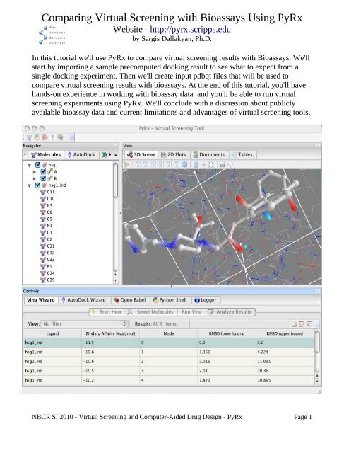
Comparing Virtual Screening with Bioassays Using PyRx
Website - http://pyrx.scripps.edu
by Sargis Dallakyan, Ph.D.
In this tutorial we'll use PyRx to compare virtual screening results with Bioassays. We'll
start by importing a sample precomputed docking result to see what to expect from a
single docking experiment. Then we'll create input pdbqt files that will be used to
compare virtual screening results with bioassays. At the end of this tutorial, you'll have
hands-on experience in working with bioassay data and you'll be able to run virtual
screening experiments using PyRx. We'll conclude with a discussion about publicly
available bioassay data and current limitations and advantages of virtual screening tools.
NBCR SI 2010 - Virtual Screening and Computer-Aided Drug Design - PyRx Page 1

Prerequisite: PyRx - http://pyrx.scripps.edu/downloads
Since PyRx is installed on all iMacs in this training room, we'll start by running it
from the /Applications folder or from the Dock. Users can also install PyRx on their
personal laptops by going to the download page for PyRx, at the above URL.
Part 1: AutoDock Wizard
In this part we'll do a dry run of the AutoDock Wizard, using precomputed docking
results.
Exercise 1: Importing Sample Data
Use the File -> Import menu, select Workspace Tarball – Remote File, click Next,
then click Finish. Wait for the Import Completed Successfully dialog and press OK.
PyRx extracts sample data and displays the
directory structure for the Ligands and the
Macromolecules folders using the AutoDock tab
under the Navigator panel shown on the right.
Click on the arrow next to hsg1 to expand or
contract the folders. As you can see from this
example, PyRx creates a folder for each target
within the Macromolecules folder, where it
stores the docking log (dlg) files. Double-click
on a pdbqt file in this widget to show the
corresponding molecule in a 3D Scene.
Control+click on any of the files in the
AutoDock tab and you'll see a menu of options
such as:
Edit Opens file in Documents editor
Delete deletes files or directories
Properties shows the path on this hard drive
Refresh Refreshes directory tree
There are additional options called Display and
Display (Mayavi) for pdbqt and for map files,
respectively, which we will cover later on.
Before we work with the AutoDock Wizard,
let's learn how to transform molecules in the
3D Scene.
NBCR SI 2010 - Virtual Screening and Computer-Aided Drug Design - PyRx Page 2

Mouse and Key Bindings
In this training room, Mac mouse preferences are set to emulate a 3-button mouse. This
means that clicking on the top-right part (i.e., the Secondary Button) emulates the rightmouse
click. Also, Button 3 act as a scroll wheel that can be used to zoom in and out in
a 3D Scene.
PyRx uses Mayavi for the 3D Scenes, and it uses the same mechanism to manipulate 3D
objects in the scene. The following is taken from the Mayavi v3.3.2 documentation to
describe interactions with the Mouse:
The view in the scene can be changed by using various mouse actions. Usually these
changes are accomplished by holding down a mouse button while dragging the mouse:
• holding the left mouse button down and dragging will rotate the camera/actor in the
direction moved.
• Holding down “SHIFT” when doing this will pan the scene – just
like the middle button.
• Holding down “CONTROL” will rotate around the camera’s axis
(roll).
• Holding down “SHIFT” and “CONTROL” and dragging up will
zoom in, while dragging down will zoom out. This is similar to
pressing the right mouse button.
• holding the right mouse button down and dragging upwards will zoom in (or
increase the actor's scale), and dragging downwards will zoom out (or reduce scale).
• holding the middle mouse button down and dragging will pan the scene or translate
the object.
• Rotating the mouse wheel upwards will zoom in and downwards will zoom out.
Users can also press the 'r' key on the keyboard to reset the camera's focal point and
position. Read the Mayavi User Guide for a complete list of features:
http://code.enthought.com/projects/mayavi/docs/development/html/mayavi/application.h
tml#interaction-with-the-scene
NBCR SI 2010 - Virtual Screening and Computer-Aided Drug Design - PyRx Page 3

Exercise 2: Using the AutoDock Wizard
Click on the AutoDock Wizard tab under the Controls panel to see the widget shown
above. There are 3 different execution modes that PyRx currently supports: (1) Local is
disabled by default. It is activated when PyRx finds autodock binaries in your “path”.
You can also use Edit -> Preferences... to tell PyRx where to find the autodock and
autogrid binaries. (2) Cluster execution mode is also disabled, since we don't have the
qsub command in our path, which can submit batch jobs to a cluster. (3) Remote mode
is always enabled, and it uses web services provided by the National Biomedical
Computation Resource (http://ws.nbcr.net) to run remote AutoDock jobs.
Note that starting with PyRx 0.6 there is a new Vina Wizard, which is selected by
default. Since Vina binaries are automatically distributed with PyRx, the Local mode for
Vina is enabled by default. There is no Remote mode available for Vina in PyRx, but
Vina web services might become available through ws.nbcr.net in the future.
Exercise 3: Select Molecules
Follow the instructions on the screen. Select ind.pdbqt from the Ligands folder, and
select the hsg1 folder or the hsg1.pdbqt file from the Macromolecules folder. Click
Forward to go to the next exercise.
NBCR SI 2010 - Virtual Screening and Computer-Aided Drug Design - PyRx Page 4

Exercise 4: Run AutoGrid
In this step you'll see a grid box in the 3D Scene and a Run AutoGrid page under the
AutoDock Wizard. You can move the spherical handles of the grid box to adjust the
dimensions for the AutoGrid maps. Click on the Maximize button if you want to
enclose the entire molecule in the gridbox (i.e., if you do not know the location of the
binding site you want to target). Click on Reset to restore the grid dimensions back to
40x40x40 and to reset the box's center to the geometric center of the molecule.
Click Forward to continue.
Note: since we already have precomputed grid maps for this example, PyRx won't run
autogrid again. However, if we didn't have the grid maps, or if the dimensions of the
grid maps had been changed, then the Forward button would start an autogrid run. You
can click on the Run AutoGrid button if you would like to run autogrid in this step,
regardless of the available grid maps.
NBCR SI 2010 - Virtual Screening and Computer-Aided Drug Design - PyRx Page 5

Exercise 5: Run AutoDock
The Run AutoDock tab allows you to select among four docking algorithms available
in AutoDock. Click on Docking Parameters... to see the run parameters that can be
changed. Users who are familiar with AutoDock can adjust these parameters to their
liking. In particular, the maximum number of energy evaluations is set to 250,000 by
default, which results in a short run. Users can choose either the short, medium, long or
custom value for this parameter. Click on OK to close this window, then click the
Forward button to go to the “analyze results” section. Similar to the Run AutoGrid
page, PyRx opens precomputed dlg files, when they are available. Note: the last
sentence of the status bar reads Click Forward to Analyze Results. If we did not have
any precomputed dlg files for this protein-ligand complex, then this line would have
read Click Forward to Run AutoDock, instead. Since we already imported the
precomputed dlg file during Exercise 1, we can now go to the next exercise, where we'll
see how docking results can be analyzed.
NBCR SI 2010 - Virtual Screening and Computer-Aided Drug Design - PyRx Page 6

Exercise 6: Analyze Results
The Analyze Results page is where the final docking results are presented. For the
AutoDock Wizard, this page contains a table, as shown above. Users can sort this table
according to the values in any particular column. Click on a row to see the
corresponding docking pose in the 3D Scene. You can also export the numerical results
as a Comma-Separated Values (CSV) file, which can later be imported into a third-party
spreadsheet application.
Before we start the next part, let's remove all the files from the workspace. Click on
the AutoDock tab in the Navigator window, and use Shift + the mouse to select all the
files in the Ligands folder. Right-click, select Delete, and click Yes to confirm.
This concludes the case study of docking a single ligand to a single receptor with
AutoDock. In the next part of the tutorial, we'll use AutoDock Vina and data from
PubChem's BioAssays to do a virtual screen and to compare the computational results
with the wet-lab experiment.
NBCR SI 2010 - Virtual Screening and Computer-Aided Drug Design - PyRx Page 7

Part 2: Virtual Screening and BioAssay
To compare our in silico screen with a real in vitro experiment, we'll use
15-Hydroxyprostaglandin Dehydrogenase (PDB ID: 2GDZ) as our target. This is one of
the few proteins that has both a 3D structure as well as bioassay data available in
PubChem. We'll start by preparing the input files for our virtual screen.
Exercise 1: Prepare the Input Structures
Click on File -> Import, click Next, enter 2gdz for the PDB ID, and click Finish.
Right-Click on 2gdz in the Molecules tab, and select
AutoDock -> Make Macromolecule. This opens up a dialog box that can be used to
select amongst alternate conformations. Click OK to let PyRx (1) create a 2gdz folder
under Macromolecules and (2) put 2gdz.pdbqt in it.
Click on the Open Babel tab under the Controls pane. Click on the first icon
on the toolbar, and open Desktop/PyRx2010/3D.sdf. You can also download this file
from the web by following the links to this PubChem BioAssay from the PyRx blog:
http://pyrx.scripps.edu/blog/81-thermal-shift-assay-for-inhibitors-of-hpgd
Right-Click on any of the entries inside the Open Babel widget, and select Convert All
to AutoDock Ligand (pdbqt). This opens a progress dialog box and shows the pdbqt
files created in the Ligands folder. Now that we have the input pdbqt structures, we are
ready to use the Vina Wizard.
NBCR SI 2010 - Virtual Screening and Computer-Aided Drug Design - PyRx Page 8

Exercise 2: Using the Vina Wizard
Click on the Vina Wizard tab under the Controls pane. The first page for the Vina
Wizard is similar to the AutoDock Wizard, except that there are 2 execution modes,
instead of 3 (i.e., there are currently no remote web services for Vina). Also, since Vina
binaries are distributed within PyRx, the Local execution mode is enabled by default.
Click on the Start button to begin. On the Select Molecules page, use
Shift + the mouse to select all the ligands, select 2gdz under the Macromolecules
folder, and click Forward. On the Run Vina page, click the Maximize button to make
the Vina search space large enough to include all the atoms from our target.
Click Forward to start the virtual screen. PyRx now loops through all the selected
ligands and runs Vina for each of them. You'll see a new tab in the View pane where
PyRx displays: the command line used to start Vina, the working directory, and the
output from Vina. Docking each ligand takes around a minute; thus, the entire virtual
screen might take an hour to finish. You can click on Analyze Results to see the Vina
results as they are created. If you have access to a computer cluster with the Portable
Batch System (PBS) or Sun Grid Engine (SGE) installed, then you'll have the qsub
command in your path, which will allow you to run virtual screens on a cluster. In this
case (when qsub is in your path), PyRx enables the Cluster execution mode on the start
page. You can also try the AutoDock Wizard with the Remote execution mode later.
NBCR SI 2010 - Virtual Screening and Computer-Aided Drug Design - PyRx Page 9

Exercise 3: Comparing Docking Results with BioAssay
PyRx stores virtual screening results in a multi-table database that you can access by
clicking on the Tables tab under the View pane. This table widget provides a bird's-eye
view of your workspace, and it includes tables for Ligands, Targets, and Docking
Results. In addition, it has an option to import other tables that are in the Comma-
Separated Values (CSV) format, such as bioassay data (or data from your own assays).
This SQLite3 database is stored in ~/.mgltools/PyRx/db.sqlite3. To save some space,
only the lowest binding energies per job are stored in the Docking Results table. PyRx
provides an option to save these tables as CSV files ( icon on the toolbar).
Click the icon on the toolbar to open the Data Plotting Dialog. By default, this
widget opens with the Docking Results table selected, and it plots Binding Energy
versus Ligand ID. If PyRx can't convert all entries in a given column into integer or
floating point numbers, then it will use the index (row) of the entries, instead. Click the
drop-down menu under Select
Table, and select Ligands. Then
select Torsional DOF for the Y
Column and Size for the X
Column. This creates the figure
shown on the right. Click OK to
store this figure under the 2D
Plots tab. You can then zoom,
pan, and save this figure using
matplotlib icons on the toolbar.
NBCR SI 2010 - Virtual Screening and Computer-Aided Drug Design - PyRx Page 10

Click the icon on the Tables tab, and open Desktop/PyRx2010/BioAssay.cvs. You
can also download this file from the web by following the links to this PubChem
BioAssay from the PyRx blog:
http://pyrx.scripps.edu/blog/81-thermal-shift-assay-for-inhibitors-of-hpgd
Click the icon again, and select Docking Results under Select Table. You'll see a
plot similar to the one shown above. Since we now have a fourth table that contains an
Outcome column with “Active”, “Inconclusive,” or “Inactive” entries, PyRx checks to
see if the compound IDs (CID) in this table match the CIDs under the Docking Results
table's Ligand column. If so, PyRx plots Active entries in red and Inactive entries in
blue. In addition, PyRx plots a Receiver Operating Characteristic (ROC) curve, where
you can see the True Positive Rate (Sensitivity) plotted against the False Positive Rate
(1 – Specificity). ROC curves are very useful when comparing virtual screening results
with in vitro experiments (especially when you are developing docking algorithms or
testing different parameters). For instance, if we had to pick randomly from our ligand
library, we would get 0.5 for the area under the ROC curve (AUC) – i.e., the diagonal
dotted line. In this particular case (this Thermal Shift Assay for Inhibitors of 15-
Hydroxyprostaglandin Dehydrogenase), we get perfect results with AutoDock: binding
energies for all active compounds are more favorable (lower) than the binding energies
for the two inactive compounds. This gives us an AUC of 1, as displayed in the above
figure.
Read the PyRx blog for other examples of ROC curves: http://pyrx.scripps.edu/blog
Useful Resources
The Curious Wavefunction Blog -
http://wavefunction.fieldofscience.com
In the Pipeline Blog - http://pipeline.corante.com
?Questions?
NBCR SI 2010 - Virtual Screening and Computer-Aided Drug Design - PyRx Page 11