(CRAM) For Wetlands User's Manual Version 5.0.2

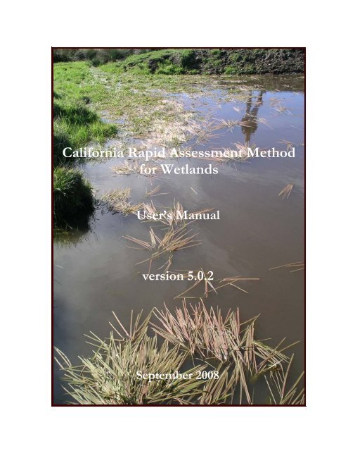
California Rapid Assessment Method 

for Wetlands 

User’s Manual 

version 5.0.2 

September 2008

This report should be cited as: 

Collins, J.N., E.D. Stein, M. Sutula, R. Clark, A.E. Fetscher, L. Grenier, C. Grosso, and A. 

Wiskind. 2008. California Rapid Assessment Method (CRAM) for Wetlands, v. 5.0.2. 157 pp. 

Funding for CRAM development was provided to the San Francisco Estuary Institute, the 

Southern California Coastal Water Research Project, and the California Coastal Commission 

through USEPA contracts CD-96911101-0, CD-96911201-0, and CD-96911301-1, respectively. 

The contents of this document do not necessarily reflect the views and policies of the EPA nor 

does the mention of trade names or commercial products constitute endorsement or 

recommendation for use. 

Cover Photograph: Joshua N. Collins

California Rapid Assessment Method for Wetlands v. 5.0.2 

California Rapid Assessment Method (CRAM) 

For Wetlands 

User’s Manual 

Version 5.0.2 

September 2008 

Joshua N. Collins, Ph.D., San Francisco Estuary Institute 1 

Eric Stein, Dr. Env., Southern California Coastal Water Research Project 2 

Martha Sutula, Ph.D., Southern California Coastal Water Research Project 2 

Ross Clark, California Coastal Commission 3 

A. Elizabeth Fetscher, Ph.D., Southern California Coastal Water Research Project 2 

Letitia Grenier, Ph.D., San Francisco Estuary Institute 1 

Cristina Grosso, MS, San Francisco Estuary Institute 1 

Adam Wiskind, Moss Landing Marine Laboratories 4 

1 San Francisco Estuary Institute 

7770 Pardee Lane 

Oakland, California 94621 

www.sfei.org 

2 Southern California Coastal 

Water Research Project 

3535 Harbor Boulevard, Suite 110 

Costa Mesa, California 92626 

www.sccwrp.org 

3 California Coastal Commission 

Central Coast District Office 

725 Front Street, Suite 300 

Santa Cruz, CA 95060 

www.coastal.ca.gov 

4 Moss Landing Marine Laboratories 

8272 Moss Landing Road 

Moss Landing, California, 95039 

www.mlml.calstate.edu 

Volume Two: Worksheets and Data sheets for assembling hardcopy field books, and 

CRAM Software 1.0.0 (an electronic version of CRAM 5.0.2) 

are available at www.cramwetlands.org


CRAM Core Team and Regional Team members 

Joshua N. Collins


VERSION HISTORY OF CRAM METHODOLOGY 

Version 5.0.2 released 9/30/08 

Changes in this version: 

Added section on version history of CRAM methodology and fixed typos 

Added paragraph in Section 2.3.1 to explain separation of assessments of condition and 

stress 

Added note to Section 3.2.2.2 that the depressional module was primarily based on 

perennial depressional wetlands and caution should be applied in the interpretation of 

scores in seasonal depressional wetlands 

Corrected text in various Sections to eliminate inconsistencies in terminology 

Updated figures in Chapter 3 

Revised the ratings for scoring Structural Patch Richness for Estuarine wetlands 

Version 5.0.1 released 10/17/07 


Minor wording changes for clarification 



Version numbering changed from 4.6 to 5.0—no other changes 

Version 4.6 released 9/10/07 


Substantial changes in nearly all areas 

Changes to metrics included: 

Wording changes for clarification 

Added a second “B” rating for scoring Landscape Connectivity for Riverine wetlands 

Revised the “C” and “D” ratings for scoring Number of Plant Layers Present for 

Slope and Confined Riverine wetlands 

Versions 4.3 - 4.5 

Internal development versions 



Reorganized volume 2 into three sections: Assessment Forms, Narratives, Tables & 

Figures; typos fixed 



Added citation to title page and fixed typos 



i


Vol 1, p. 15: Table 2.2, added new metric name Plant Community and bulleted its four 

component submetrics 

Vol 1, p. 36: Added language prescribing the calculation of mean submetric score in 

order to arrive at Plant Community metric value; in Table 3.8, changed expected 

maximum value of Biotic Structure attribute from 84 to 36 for Playas and Vernal Pools 

and 48 for all other wetland classes 

Vol 1, pp. 68-71: Changed “metric” to “submetric” for discussion of the four submetrics 

of the Plant Community metric 

Vol 2, pp.145-6: removed wrackline or organic debris in channel or on floodplain from 

worksheet 2 since this patch type is not expected in playas 

Vol 2, p. 55: Revised “D” narrative for number of plants layers present from "No layers 

are present" to "0-1 layer is present" 

Vol 2, pp. 133, 149, 166: Removed shading from scoring sheet for Interspersion and 

Zonation since this metric is assessed for vernal pools and playas 

Vol 2: Revised scoring forms to incorporate Plant Community metric 



Split into two volumes: main manual and assessment forms 

Created separate volume for assessment forms - all supporting documents included with 

each class 

Updated entrenchment ratio and hydrologic connectivity metric bins 

Revised bins for percent co-dominant species that are non-native 

Added confined v. unconfined diagram 

Revised scoring to a 1-12 scale for all metrics 



Separated estuarine class into two sub-classes: saline and non-saline 


ii

California Rapid Assessment Method for Wetlands v. 5.0.2 – Acknowledgments 

ACKNOWLEDGMENTS 

The authors would like to credit the Washington State Wetland Rating System, the Ohio Rapid 

Assessment Method for Wetlands, and the Hydrogeomorphic (HGM) Functional Assessment 

Method for providing a foundation upon which to create the California Rapid Assessment 

Method for Wetlands (CRAM). 

CRAM could not have been developed without the championship of Paul Jones (USEPA 

Region 9) and Richard Sumner (USEPA Office of Research and Development), technical 

guidance from Mary Kentula (USEPA Office of Research and Development), the inspirational 

successes of John Mack (Ohio EPA) and M. Siobhan Fennessy (Kenyon College), plus the 

abundant advice and review provided by the CRAM Core Team and Regional Teams. 

Core Team 

Aaron Allen USACOE-LA District Ruben Guieb SWRCB 

Richard Ambrose UCLA Raymond Jay RWQCB-Region 4 

Oscar Balaguer SWRCB Michael Jewell USACOE-Sacramento Dist. 

Andree Breaux RWQCB-Region 2 Steven John USEPA 

Robert Burton MLML Paul Jones USEPA 

John Callaway USF Molly Martindale USACOE – SF District 

Elizabeth Chattin County of Ventura Dan Martel USACOE – SF District 

Ross Clark CCC Sarah Pearce SFEI 

Bobby Jo Close CCC Chris Potter State Resources Agency 

Joshua Collins SFEI Eric Stein SCCWRP 

John Dixon CCC Don Stevens OSU 

Betty Fetscher SCCWRP Richard Sumner USEPA 

Letitia Grenier SFEI Martha Sutula SCCWRP 

Cristina Grosso SFEI Adam Wiskind MLML 

Central Coast Regional Team 

Mary Adams RWQCB, Region 3 Dave Highland CDFG 

Alyson Aquino CPI Bill Hoffman Morro Bay NEP 

Chris Berry City of Santa Cruz Matt Johnson Santa Cruz County 

Rob Burton MLML Ann Kitajima Morro Bay NEP 

Cammy Chabre Elkhorn Slough NERR Cheryl Lesinski Morro Bay NEP 

Becky Christensen Elkhorn Slough NERR Stacey Smith California Conservation Corps 

Ross Clark CCC Eric Van Dyke Elkhorn Slough NERR 

Bobby Jo Close CCC Kerstin Wasson Elkhorn Slough NERR 

Chris Coburn MBNMS Adam Wiskind MLML 

Kevin Contreras Elkhorn Slough Foundation David Wolff David Wolff Environmental 

Gage Dayton MLML Andrea Woolfolk Elkhorn Slough NERR 

Rebecca Ellin CCWGIS Susie Worcester CSU Monterey Bay 

North Coast Regional Team 

Annie Eicher UC Sea Grant Extension Chad Roberts HBHRCD 

Stephanie Morrissette Mad River Biologists Jeff Robinson HBHRCD 

Renee Pasquinelli CDPR 

iii

California Rapid Assessment Method for Wetlands v. 5.0.2 – Acknowledgments 

San Francisco Bay Area Regional Team 

Elaine Blok USFWS-NWI Paul Jones USEPA - Region 9 

Andree Breaux RWQCB - Region 2 Tom Kucera Kucera Associates 

John Callaway USF Karl Malamud-Roam CMVCA 

Josh Collins SFEI Dan Martel USACOE – SF District 

Steve Culberson CDWR Molly Martindale USACOE – SF District 

Joe Didonato EBRPD Nadav Nur PRBO 

Giselle Downard USFWS Lorraine Parsons USNPS 

Jules Evens Avocet Research Sarah Pearce SFEI 

Tom Gardali PRBO Louisa Squires SCVWD 

Letitia Grenier SFEI Eric Tattersall CDFG 

Cristina Grosso SFEI Nils Warnock PRBO 

Southern California Regional Team 

Darcy Aston WRP SB Task Force Spencer MacNeill Aspen Environmental 

Karen Bane SCC Mike Porter RWQCB-Region 9 

Shirley Birosik RWQCB - Region 4 Bruce Posthumus RWQCB-Region 9 

Liz Chattin Ventura County David Pritchett WRP SB Task Force 

Bryant Chesney NOAA Ruben Ramirez Cadre Environmental 

Jae Chung USACOE Lorraine Rubin Ventura County 

Rosi Dagit RCDSMM Mary Anne Skorpanich OCPFRD 

Sabrina Drill UC Extension Eric Stein SCCWRP 

Corrice Farrar USACOE- LA District Martha Sutula SCCWRP 

Doug Gibson SELC Kelly Schmoker RMC 

Ryan Henry PCR Wanda Smith RWQCB - Region 8 

Mike Kleinfelter Independent Consultant Bob Thiel WRP SB Task Force 

Erik Larsen URS Corp. Dick Zembal OCWD 

Dave Lawhead CDFG David Zoutendyk USFWS 

Mary Loquvam LASGRWC 

Organization Codes 

CCC Ca Coastal Commission OCPFRD Orange County Public Facilities & Resources Dept 

CCWGIS Central Coast Wetlands GIS Project PCR PCR Services Corporation 

CDFG Ca Department of Fish and Game PRBO Point Reyes bird Observatory 

CDPR CA Department of Parks and Recreation RCDSMM 

Resource Conservation District of the Santa 

iv 

Monica Mountains 

CDWR Ca Department of Water Resources RMC 

San Gabriel & Lower Los Angeles Rivers and 

Mountains Conservancy 

CMVCA Ca Mosquito & Vector Control Assoc. RWQCB Regional Water Quality Control Board 

CPI Ca Polytech Institute SCC South Coast Ca Coastal Conservancy 

CSU Ca State University SCCRPP Southern. Ca Coastal Water Research Project 

EBRPD East Bay Regional Park District SCVWD Santa Clara Valley Water District 

HBHRCD 

Humboldt Bay Harbor, Recreation and 

Conservation District 

SELC Southern Environmental Law Center 

LASGRWC 

Los Angeles & San Gabriel Rivers 

SFEI San Francisco Estuary Institute 

Watershed Council 

MBNMS Monterey Bay National Marine Sanctuary SWRCB Ca State Water Resources Control Board 

MLML Moss Landing Marine Laboratory UC University of California 

NEP National Estuary Program USACOE US Army Corps of Engineers 

NERR National Estuary Research Reserve USEPA US Environmental Protection Agency 

NWI National Wetland Inventory USF University of San Francisco 

OCWD Orange County Water District USFWS US Fish and Wildlife Service 

OSU Oregon State University USNPS US National Park Service

California Rapid Assessment Method for Wetlands v. 5.0.2 – Table Contents 

TABLE OF CONTENTS 

Version History of CRAM Methodology ..........................................................................................i 

Acknowledgments ...............................................................................................................................iii 

EXECUTIVE SUMMARY ................................................................................................................1 

CHAPTER 1: NEED, GOAL, STRATEGIC CONTEXT, INTENDED USES, AND 

GEOGRAPHIC SCOPE ........................................................................................3 

1.0 Introduction.............................................................................................................................3 

1.1 Statement of Need..................................................................................................................3 

1.2 Justification for Rapid Assessment.......................................................................................3 

1.3 Goal and Intended Use..........................................................................................................5 

1.4 Related Rapid Assessment Efforts in California and Other States .................................6 

1.5 Geographic Scope...................................................................................................................6 

1.6 Supporting Information Systems..........................................................................................6 

1.7 Organization and Coordination to Develop CRAM .........................................................7 

1.7.1 Core Team...............................................................................................................7 

1.7.2 Regional Teams ......................................................................................................7 

CHAPTER 2: KEY TERMS, CONCEPTS, ASSUMPTIONS, AND 

DEVELOPMENTAL PROCESS .........................................................................9 

2.0 Overview..................................................................................................................................9 

2.1 Key Terms................................................................................................................................9 

2.2 Conceptual Framework....................................................................................................... 10 

2.2.1 Management Framework................................................................................... 10 

2.2.2 Rapid Assessment ............................................................................................... 11 

2.2.3 Forcing Functions, Stress, Buffer, and Condition ......................................... 11 

2.2.4 Condition, Ecological Service, and CRAM Scores ........................................ 11 

2.3 Developmental Framework................................................................................................ 13 

2.3.1 Basic Design......................................................................................................... 13 

2.3.2 Calibration............................................................................................................ 13 

2.3.3 Validation ............................................................................................................. 14 

CHAPTER 3: PROCEDURES FOR USING CRAM .............................................................. 17 

3.0 Summary................................................................................................................................ 17 

3.1 Step 1: Assemble Background Information..................................................................... 17 

3.2 Step 2: Classify the Wetland and Riparian Areas ............................................................ 18 

3.2.1 General Definitions of Wetlands and Riparian Areas ................................... 18 

3.2.2 Wetland Typology............................................................................................... 20 

3.4 Step 4: Verify the Appropriate Assessment Window..................................................... 26 

3.5 Step 5: Establish the Assessment Area (AA)................................................................... 27 

3.5.1 Hydro-geomorphic Integrity ............................................................................. 27 

3.5.2 AA Size................................................................................................................. 28 

v


3.5.3 Assessment Purpose ........................................................................................... 30 

3.5.4 Special Considerations for Riverine Wetlands Including Riparian Areas... 32 

3.5.5 Special Considerations for Estuarine Wetlands.............................................. 33 

3.5.6 Special Considerations for Vernal Pool Systems............................................ 33 

3.5.7 Special Considerations for Post-assessment Analysis.................................... 35 

3.5.8 Special Considerations for Assessing Projects................................................ 35 

3.6 Step 6: Conduct Initial Office Assessment of Condition Metrics and Stressors........ 36 

3.7 Step 7: Conduct Field Assessment of Condition Metrics and Stressors...................... 37 

3.8 Step 8: Complete CRAM Scores and Basic QA/QC Procedures ................................ 37 

3.8.1 Calculating CRAM Scores.................................................................................. 37 

3.8.2 Initial QA/QC Procedures for Data Collectors............................................. 40 

3.8.3 Initial Quality Control Procedures for Data Managers ................................. 40 

3.9 Step 9: Upload Assessment Data and Results ................................................................. 41 

CHAPTER 4: GUIDELINES FOR SCORING CRAM METRICS...................................... 43 

4.0 Summary................................................................................................................................ 43 

4.1 Attribute 1: Buffer and Landscape Context..................................................................... 43 

4.1.1 Landscape Connectivity ..................................................................................... 43 

4.1.2 Percent of AA with Buffer ................................................................................ 47 

4.1.3 Average Buffer Width ........................................................................................ 49 

4.1.4 Buffer Condition................................................................................................. 52 

4.2 Attribute 2: Hydrology........................................................................................................ 53 

4.2.1 Water Source........................................................................................................ 53 

4.2.2 Hydroperiod or Channel Stability..................................................................... 56 

4.2.3 Hydrologic Connectivity.................................................................................... 62 

4.3 Attribute 3: Physical Structure ........................................................................................... 65 

4.3.1 Structural Patch Richness .................................................................................. 65 

4.3.2 Topographic Complexity ................................................................................... 71 

4.4 Attribute 4: Biotic Structure ............................................................................................... 74 

4.4.1 Plant Community Metric........................................................................................ 74 

4.4.2 Horizontal Interspersion and Zonation........................................................... 83 

4.4.3 Vertical Biotic Structure..................................................................................... 87 

CHAPTER 5: GUIDELINES TO COMPLETE STRESSOR CHECKLISTS.................... 91 

REFERENCES ................................................................................................................................. 95 

APPENDIX I: PROTOCOL FOR PROJECT ASSESSMENT BASED ON CRAM...... 101 

APPENDIX II: FLOW CHART TO DETERMINE PLANT DOMINANCE................ 107 

APPENDIX III: GLOSSARY..................................................................................................... 109 

APPENDIX IV: ACRONYM LIST........................................................................................... 115 

APPENDIX V: INVASIVE PLANT SPECIES LIST............................................................ 117 

Appendix V-A: List of California Plant Species (alphabetized by plant species)................ 117 

vi


Appendix V-B: List of California Plant Species (alphabetized by common name)............ 135 

APPENDIX VI: VERNAL POOL PLANT SPECIES LIST................................................ 153 

vii


LIST OF FIGURES 

Figure 2.1: Spatial hierarchy of factors that control wetland conditions...................................12 

Figure 2.2: Spatial hierarchy of stressors, buffers, and wetland condition................................12 

Figure 3.1: Using backshores, foreshores, and wetland boundaries to wetlands .....................19 

Figure 3.2: Flowchart to determine wetland type and sub-type..................................................21 

Figure 3.3: Illustrations of riverine confinement and entrenchment. ........................................22 

Figure 3.4: Cross-section of riverine AA........................................................................................32 

Figure 3.5: Example of an estuarine wetland and a characteristic Assessment Area...............33 

Figure 3.6: Example map of one vernal pool system and its component elements. ...............34 

Figure 3.7: Example graphs for displaying CRAM results. .........................................................39 

Figure 4.1: Method to assess Landscape Connectivity of riverine wetlands.. ..........................46 

Figure 4.2: Diagram of buffer and non-buffer land cover types. ...............................................48 

Figure 4.3: Examples of method used to estimate Buffer Width...............................................50 

Figure 4.4: Diagram of approach to estimate Buffer Width for Riverine AAs. .......................51 

Figure 4.5: Parameters of Channel entrenchment. .......................................................................63 

Figure 4.6: Scale-independent schematic profiles of Topographic Complexity.......................72 

Figure 4.7: Diagram of plant zone interspersion for Lacustrine, Depressional, 

Playas, and Slope wetlands ...........................................................................................83 

Figure 4.8: Diagram of plant zone interspersion for Individual Vernal Pools. ........................84 

Figure 4.9: Diagram of plant zone interspersion for Riverine wetlands....................................84 

Figure 4.10: Diagrams of plant zone interspersion for Perennial Saline, Non-saline, 

and Seasonal Estuarine wetlands.................................................................................85 

Figure 4.11: Diagrams of vertical interspersion of plant layers for Riverine wetlands 

and for Depressional and Lacustrine wetlands having Tall or Very Tall 

plant layers. .....................................................................................................................88 

Figure 4.12: Diagrams of entrained plant canopies in ESturaine wetlands and in 

Depressional and Lacustrine, wetlands dominated by emergent 

monocots or lacking Tall and Very Tall plant layers.. ..............................................89 

viii


LIST OF TABLES 

Table 4.1: Basic outline of CRAM development................................................................................13 

Table 2.2: CRAM Site Attributes and Metrics. ...................................................................................14 

Table 2.3: Expected relationships among CRAM attributes, metrics, and key services……... ..15 

Table 3.1: Steps for using CRAM. ........................................................................................................17 

Table 3.2: Example of background materials......................................................................................17 

Table 3.3: Guidelines to delineate a wetland for the purpose of CRAM........................................19 

Table 3.4: The CRAM Wetland Typology...........................................................................................20 

Table 3.5: Examples of features that should be used to delineate AA boundaries. ........................29 

Table 3.6: Examples of features that should not be used to delineate any AAs.............................29 

Table 3.7: Preferred and minimum AA sizes for each wetland type. ..............................................30 

Table 3.8: Guidelines for determining the number of AAs per wetland. .......................................31 

Table 3.9: Steps to delineate a vernal pool system and its component large and small pools….34 

Table 3.10: CRAM metrics suitable for pre-site visit draft assessment.............................................36 

Table 3.11: Steps to calculate attribute scores and AA scores............................................................38 

Table 3.12: Recommended topics of initial QA/QC...........................................................................40 

Table 4.1: Rating for Landscape Connectivity for all wetlands except Riverine............................45 

Table 4.2: Steps to assess Landscape Connectivity for riverine wetlands.......................................45 

Table 4.3: Rating for Landscape Connectivity for Riverine wetlands. ............................................46 

Table 4.4: Guidelines for identifying wetland buffers and breaks in buffers. ................................49 

Table 4.5: Rating for Percent of AA with Buffer. ..............................................................................49 

Table 4.6: Steps to estimate Buffer Width for all wetlands...............................................................50 

Table 4.7: Rating for Average Buffer Width. ......................................................................................52 

Table 4.8: Rating for Buffer Condition................................................................................................52 

Table 4.9: Rating for Water Source. .....................................................................................................55 

Table 4.10: Field Indicators of Altered Hydroperiod. .........................................................................57 

Table 4.11a: Rating of Hydroperiod for Depressional, Lacustrine, Playas, and Slope. ....................57 

Table 4.11b: Rating of Hydroperiod for Individual Vernal Pools and Pool Systems. ......................58 

Table 4.12: Rating of Hydroperiod for Perennial Estuarine wetlands. .............................................59 

Table 4.13: Rating of Hydroperiod for Seasonal Estuarine wetlands................................................59 

Table 4.14: Rating for Riverine Channel Stability.................................................................................62 

Table 4.15a: Rating of Hydrologic Connectivity for Non-confined Riverine wetlands. ..................64 

Table 4.15b: Rating of Hydrologic Connectivity for Confined Riverine wetlands............................64 

ix


Table 4.15c: Rating of Hydrologic Connectivity for Estuarine, Depressional, Lacustrine, and 

Slope wetlands, Playas, Individual Vernal Pools, and Vernal Pool Systems................64 

Table 4.16: Rating of Structural Patch Richness (based on results from worksheets)....................70 

Table 4.17: Typical indicators of Macro- and Micro-topographic Complexity................................71 

Table 4.18a: Rating of Topographic Complexity for Depressional Wetlands, Playas, 

Individual Vernal Pools, and Slope Wetlands...................................................................72 

Table 4.18b: Rating of Topographic Complexity for all Estuarine Wetlands.....................................73 

Table 4.18c: Rating of Topographic Complexity for all Riverine Wetlands.......................................73 

Table 4.18d: Rating of Topographic Complexity for Vernal Pool Systems........................................74 

Table 4.19: Ratings for submetrics of Plant Community Metric........................................................82 

Table 4.20a: Rating of Horizontal Interspersion of Plant Zones for all AAs except 

Riverine and Vernal Pool Systems. ....................................................................................86 

Table 4.20b: Rating of Horizontal Interspersion of Plant Zones for Riverine AAs. ........................86 

Table 4.20c: Rating of Horizontal Interspersion for Vernal Pool Systems. .......................................86 

Table 4.21: Rating of Vertical Biotic Structure for Riverine AAs and for Lacustrine 

and Depressional AAs supporting Tall or Very Tall plant layers ..................................88 

Table 4.22: Rating of Vertical Biotic Structure for wetlands dominated by emergent 

monocots or lacking Tall and Very Tall plant layers. ......................................................89 

Table 5.1: Wetland disturbances and conversions..............................................................................91 

x

LIST OF WORKSHEETS 

Worksheet 4.1: Landscape Connectivity Metric for All Wetlands Except Riverine........................44 

Worksheet 4.2: Landscape Connectivity Metric for Riverine Wetlands......................................... 146 

Worksheet 4.3: Calculating Average Buffer Width of AA. .................................................................51 

Worksheet 4.4: Assessing Hydroperiod for Riverine Wetlands..........................................................61 

Worksheet 4.5: Riverine Wetland Entrenchment Ratio Calculation............................................... 363 

Worksheet 4.6: Structural Patch Types for All Wetland Types, Except Vernal Pool 

Systems. ...........................................................................................................................38 

Worksheet 4.7: Structural Patch Types for Vernal Pool Systems.......................................................40 

Worksheet 4.8.1: Plant layer heights for all wetland types......................................................................57 

Worksheet 4.8.2: Co-dominant Species Richness for All Wetland Types, Except 

Confined Riverine, Slope Wetlands, Vernal Pools, and Playas.................................38 

Worksheet 4.8.3: Co-dominant Species Richness for Confined Riverine and Slope 

Wetlands ...........................................................................................................................38 

Worksheet 4.8.4: Co-dominant Plant Species in Vernal Pool Systems – Large Pools. ......................49 

Worksheet 4.8.5: Co-dominant Plant Species in Vernal Pool Systems – Small Pools .......................50 

Worksheet 4.8.6: Co-dominant Plant Species in Playas and Individual Vernal Pools........................81 

Worksheet 4.8.7: Native Plant Species Observed in Vernal Pools or Vernal Pool 

Systems. ...........................................................................................................................81 

Worksheet 4.8.8: Summary Submetric Scores for Vernal Pool Systems. .............................................81 

Worksheet 5.1: Stressor Checklist Worksheet.......................................................................................73 

xi

Seasonal estuarine wetland, Abbotts Lagoon, Point Reyes National Seashore 

xii 

Joshua N. Collins

California Rapid Assessment Method for Wetlands v. 5.0.2 – Executive Summary 

EXECUTIVE SUMMARY 

Large amounts of public funds and human resources are being invested in the protection, 

restoration, creation, and enhancement of wetlands in California. The State needs to be able to 

track the extent and condition of these habitats to evaluate the investments in them now and 

into the future. The community of wetland scientists, managers, and regulators needs to be able 

to answer the questions: where are the wetland areas and how are they doing? This need is 

clearly indicated by the California State Wetlands Conservation Policy. 

A consortium of local, state and federal authorities has been developing new tools to increase 

the State’s capacity to monitor its wetlands. The effort is guided by the three-level framework for 

surface water monitoring and assessment recently issued to the state by the USEPA (USEPA 

2006). Level 1 consists of habitat inventories and landscape profiles based on the statewide 

wetland inventory as mandated by California Assembly Bill 2286, the statewide riparian 

inventory as planned by the Riparian Habitat Joint Venture, and the Wetland Trackers of the 

Regional Data Centers being developed by the State Water Resources Control Board and others 

as part of the California Environmental Data Exchange Network. Level 2 consists of rapid 

assessment of wetland condition in relation to the broadest suite possible of ecological and social 

services and beneficial uses. Level 3 consists of standardized protocols for intensive-quantitative 

assessment of selected services and to validate and explain Level 1 and Level 2 methods and 

results. All three levels are to be supported by data management systems that enable the State to 

compile local and regional Level 1-3 data into statewide summary reports. Level 1 and Level 2 

methods are supported by open-source, web-based information systems (wetlandtracker.org and 

cramwetlands.org) that are consistent with existing state and federal environmental databases. 

Level 3 protocols and results will be added to these information systems as they are developed. 

This manual focuses on the California Rapid Assessment Method. CRAM is being developed as 

a cost-effective and scientifically defensible Level 2 method for monitoring the conditions of 

wetlands throughout California. The CRAM web site (www.cramwetlands.org) provides access 

to an electronic version of this manual, training materials, eCRAM (the downloadable software 

that eliminates the need for taking a hardcopy version of CRAM into the field), and the CRAM 

database. CRAM results can be uploaded to the database, viewed, and retrieved via the CRAM 

web site. CRAM, eCRAM, and the supporting web sites are public and non-proprietary. 

CRAM development has focused on the wetlands of coastal watersheds from Mexico to 

Oregon. These watersheds in aggregate encompass almost as much variation in climate, geology, 

and land use as the State as a whole. A special effort has been made, however, to involve 

environmental scientists and managers who are familiar with inland arid montane environments 

that are not well represented in the coastal watersheds. Seasoned staff from natural resource 

management and regulatory agencies, NGO science institutions, the private sector, and academia 

have worked together through four coastal Regional Teams and a statewide Core Team to 

provide the breadth and depth of technical and administrative experience necessary to help 

assure statewide applicability of CRAM. 

CRAM development has incorporated aspects of other approaches to habitat assessment used in 

California and elsewhere, including the Washington State Wetland Rating System (WADOE 

1993), MRAM (Burglund 1999), and ORAM (Mack 2001). CRAM also draws on concepts from 

1

California Rapid Assessment Method for Wetlands v. 5.0.2 – Executive Summary 

stream bio-assessment and wildlife assessment procedures of the California Department of Fish 

and Game, the different wetland compliance assessment methods of the San Francisco Bay 

Regional Water Quality Control Board and the Los Angeles Regional Water Quality Control 

Board, the Releve Method of the California Native Plant Society, and various HGM guidebooks 

that have been developed in California. 

In essence, CRAM enables two or more trained practitioners working together in the field for 

one half day or less to assess the overall health of a wetland by choosing the best-fit set of 

narrative descriptions of observable conditions ranging from the worst commonly observed to 

the best achievable for the type of wetland being assessed. There are four alternative descriptions 

of condition for each of fourteen metrics that are organized into four main attributes: (landscape 

context and buffer, hydrology, physical structure, and biotic structure) for each of six major 

types of wetlands recognized by CRAM (riverine wetlands, lacustrine wetlands, depressional 

wetlands, slope wetlands, playas, and estuarine wetlands). To the extent possible, CRAM has 

been standardized across all these wetland types. The differences in metrics and narrative 

descriptions between wetland types have been minimized. 

CRAM yields an overall score for each assessed area based on the component scores for the 

attributes and their metrics. The alternative narrative description for each metric has a fixed 

numerical value. An attribute score is calculated by first summing the values of the chosen 

narrative descriptions for the attribute’s component metrics, and then converting the sum into a 

percentage of the maximum possible score for the attribute. The overall score for an area is 

calculated by first summing the attribute scores, and then converting this sum into the maximum 

possible score for all attributes combined. The maximum possible score represents the best 

condition that is likely to be achieved for the type of wetland being assessed. The overall score 

for a wetland therefore indicates how it is doing relative to the best achievable conditions for 

that wetland type in the state. Local conditions can be constrained by unavoidable land uses that 

should be considered when comparing wetlands from different land use settings. 

CRAM also provides guidelines for identifying stressors that might account for low scores. 

Evident stressors are characterized as probably insignificant or strongly influencing an attribute 

score. The stressor checklist allows researchers and managers to explore possible relationships 

between condition and stress, and to identify actions to counter stressor effects. 

CRAM is a cost-effective ambient monitoring and assessment tool that can be used to assess 

condition on a variety of scales, ranging from individual wetlands to watersheds and larger 

regions. Applications could include preliminary assessments to determine the need for more 

intensive analysis; supplementing information during the evaluation of wetland condition to aid 

in regulatory review under Section 401 and 404 of the Clean Water Act or other wetland 

regulations; and assisting in the assessment of restoration or mitigation projects by providing a 

rapid means of checking progress along a particular restoration trajectory. CRAM is not intended 

to replace any existing tools or approaches to monitoring or assessment, and will be used at the 

discretion of each individual agency to complement preferred approaches. Quality assurance 

and control practices are being designed to ensure that CRAM is appropriately applied in 

ambient and regulatory applications. 

2

California Rapid Assessment Method for Wetlands v. 5.0.2 – Chapter 1 

CHAPTER 1: 

NEED, GOAL, STRATEGIC CONTEXT, INTENDED USES, AND 

GEOGRAPHIC SCOPE 

1.0 Introduction 

This document is the User’s Manual for the California Rapid Assessment Method (CRAM) for 

wetlands. CRAM is intended to assess all types of wetlands in California. The current version of 

CRAM can be used to assess all types of wetlands but cannot be used to assess riparian areas 

except in relation to riverine systems. The version of CRAM for assessing the riparian areas of 

other wetland types is not yet ready for implementation. 

Chapter 1 presents the rationale for CRAM, including why it’s needed, its primary goal, its 

strategic context, intended uses, and the geographic scope of its applicability. Chapter 2 covers 

key terms, the conceptual framework for CRAM, and its development process. Chapter 3 

describes the basic steps of the methodology. Chapter 4 provides detailed instructions with 

worksheets and datasheets for assessing a wetland using CRAM. 

1.1 Statement of Need 

As this document is being released, large amounts of public and private funds are being invested 

in policies, programs, and projects to protect, restore, and manage wetlands in California. Most 

of these investments cannot be evaluated, however, because the ambient conditions of wetlands 

are not being monitored, the methods to monitor individual wetland areas are inconsistent, and 

there is little assurance of data quality. Furthermore, the results of monitoring are not readily 

available to analysts and decision makers. CRAM is a new approach that can provide consistent, 

scientifically defensible, affordable information about wetland conditions throughout California. 

1.2 Justification for Rapid Assessment 

The three most significant obstacles to developing adequate information about the conditions of 

California wetlands are (1) the lack of regional or statewide inventories of wetlands and related 

projects; (2) the high costs of conventional assessment methods; and (3) the lack of an 

information management system to support regional or statewide wetland assessments. The 

USEPA has developed a 3-tiered framework for comprehensive assessment and monitoring of 

surface waters that can guide efforts to overcome these obstacles (USEPA 2006). 

Level 1. Level 1 consists of map-based inventories and landscape profiles of 

wetlands and related habitats in a Geographic Information System (GIS). 

Inventories are essential for locating wetlands and for describing their geographic 

distribution and abundance. While there are various efforts to map wetlands on 

regional, county, and local levels, the California State Wetland Inventory as 

mandated by Assembly Bill 2286 is the primary wetland inventory for the State. 

The statewide is inventory can be used to update the National Wetlands 

Inventory (NWI) of the USFWS and the National Hydrography Dataset (NHD) 

of the USGS, while also meeting many of the needs of regional wetland 

scientists, managers, and regulators. In addition to the inventory of wetlands, the 

State is supporting the development of web-based inventories of wetland 

3


projects (www.wetlandtracker.org) that can be used to assess the cumulative 

effect of projects on the extent and overall ambient condition of wetlands. The 

State Wetland Inventory, Riparian Inventory, and the Wetland Trackers will aid 

wetland conservation planning by showing each wetland in the context of all 

others. They will also serve as sample frames for objective, probabilistic surveys 

of the ambient condition of wetlands and for assessing the effects of projects 

and other management actions on the ambient wetland condition at various 

scales ranging from local watersheds to the State as a whole. Through the 

statewide Level 1 inventory and the Wetland Tracker, the State can overcome the 

obstacle of not having an adequate inventory of wetlands and related projects to 

track changes in their extent and condition. 

Level 2. Level 2 methods assess the existing condition of a wetland relative to its 

broadest suite of suitable functions, services, and beneficial uses, such as flood 

control, groundwater recharge, pollution control, and wildlife support, based on 

the consensus of best professional judgment. In this regard, a level 2 assessment 

represents the overall functional capacity of a wetland. To be valid, rapid 

assessments must be strongly correlated to Level 3 measures of actual functions 

or services. Once validated, Level 2 assessments can be used where Level 3 data 

are lacking or too expensive to collect. Level 2 assessments can thus lessen the 

amount and kinds of data needed to monitor wetlands across large areas over 

long periods. CRAM is the most completely developed and tested Level 2 

method for California at this time. 

Level 3. Level 3 provides quantitative data about selected functions, services, or 

beneficial uses of wetlands. Such data are needed to develop indicators, to 

develop standard techniques of data collection and analysis, to explore 

mechanisms that account for observed conditions, to validate Level 1 and 2 

methods, and to assess conditions when the results of Level 1 and Level 2 efforts 

are too general to meet the needs of wetland planners, managers, or regulators. 

CRAM is based on a growing body of scientific literature and practical experience in the rapid 

assessment of environmental conditions. Several authors have reviewed methods of wetland 

assessment (Margules and Usher 1981, Westman 1985, Lonard and Clairain 1986, Jain et al. 1993, 

Stein and Ambrose 1998, Bartoldus 1999, Carletti et al. 2004, Fennessy et al. 2004). Most 

methods differ more in the details of data collection than in overall approach. In general, the 

most useful approaches focus on the visible, physical and/or biological structure of wetlands, 

and they rank or categorize wetlands along one or more stressor gradients (Stevenson and Hauer 

2002). The indicators of condition are derived from intensive Level 3 studies that show 

relationships between the indicators, high-priority functions or ecological services of wetlands, 

and anthropogenic stress, such that the indicators can be used to assess the effects of 

management actions on wetland condition. 

Existing methods have been used to assess wetlands at a variety of spatial scales, from habitat 

patches within local projects, to watersheds and regions of various sizes. Methods that are 

designed to assess large areas, such as the Synoptic Approach (Leibowitz et al. 1992), typically 

produce coarser and more general results than site-specific methods, such as the 

Hydrogeomorphic Method (HGM; Smith et al. 1995, Smith 2000) or the Index of Biotic 

Integrity (IBI; Karr 1981). Each scale of wetland assessment provides different information. 

4


Furthermore, assessments at different scales can be used for cross-validation, thereby increasing 

confidence in the approach being used. A comprehensive wetland monitoring program might 

include a variety of methods for assessing wetlands at different scales. 

Existing methods also differ in the amount of effort and expertise they require. Methods such 

as the Wetland Rapid Assessment Procedure (WRAP; Miller and Gunsalus 1997) and the 

Descriptive Approach (USACOE 1995), are extremely rapid, whereas the Habitat Evaluation 

Procedure (HEP; USFWS 1980), the New Jersey Watershed Method (Zampella et al. 1994), and 

the Bay Area Watersheds Science Approach (WSA version 3.0, Collins et al. 1998), are much 

more demanding of time and expertise. 

None of the existing methods other than CRAM can be applied equally well to all kinds of 

wetlands in California. The HGM and the IBI are the most widely applied approaches in the 

U.S. While they are intended to be rapid, they require more time and resources than are usually 

available, and both have a somewhat limited range of applicability. For example, IBIs are 

developed separately for different ecological components of wetland ecosystems, such as 

vegetation and fish, and for different types of wetlands, such as wadeable streams and lakes. 

HGM guidebooks are similarly restricted to one type of habitat, such as vernal pools or riverine 

wetlands, and they are typically restricted to a narrowly defined bioregion. Some guidebooks are 

restricted to individual watersheds. Trial applications of rapid assessment methods developed for 

other states, including the Florida WRAP and the Ohio Rapid Assessment Method (ORAM; 

Mack 2001) in California coastal watersheds indicated that significant modifications of these 

methods would be required for their use in California, and lead to developing CRAM. 

1.3 Goal and Intended Use 

The overall goal of CRAM is to: 

Provide rapid, scientifically defensible, standardized, cost-effective assessments of the status 

and trends in the condition of wetlands and the performance of related policies, programs 

and projects throughout California. 

CRAM is being developed as a rapid assessment tool to provide information about the condition 

of a wetland and the stressors that affect that wetland. CRAM is intended for cost-effective 

ambient monitoring and assessment that can be performed on different scales, ranging from an 

individual wetland, to a watershed or a larger region. It can be used to develop a picture of 

reference condition for a particular wetland type or to create a landscape-level profile of the 

conditions of different wetlands within a region of interest. This information can then be used 

in planning wetland protection and restoration activities. Additional applications could include: 

preliminary assessments to determine the need for more traditional intensive 

analysis or monitoring; 

providing supplemental information during the evaluation of wetland condition to 

aid in regulatory review under Section 401 and 404 of the Clean Water Act, the 

Coastal Zone Management Act, Section 1600 of the Fish and Game code, or local 

government wetland regulations; and 

assisting in the monitoring and assessment of restoration or mitigation projects by 

providing a rapid means of checking progress along restoration trajectories. 

5


CRAM is not intended to replace any existing tools or approaches to monitoring or assessment, 

and will be used at the discretion of each individual agency to complement preferred 

approaches. Wetland impact analysis and compensatory mitigation planning and monitoring for 

larger wetland areas that exhibit more complex physical and biological functions will typically 

require more information than CRAM will be able to provide. 

1.4 Related Rapid Assessment Efforts in California and Other States 

Development of CRAM has incorporated concepts and methods from other wetland assessment 

programs in California and elsewhere, including the Washington State Wetland Rating System 

(WADOE 1993), MRAM (Burglund 1999), and ORAM (Mack 2001). CRAM also draws on 

concepts from stream bio-assessment and wildlife assessment procedures of the California 

Department of Fish and Game, the different wetland compliance assessment methods of the 

San Francisco Bay Regional Water Quality Control Board and the Los Angeles Regional Water 

Quality Control Board, the Releve Method of the California Native Plant Society, and various 

HGM guidebooks that are being used in California. 

1.5 Geographic Scope 

CRAM is intended for application to all kinds of wetlands throughout California. Although 

centered on coastal watersheds, CRAM development to date has involved scientists and 

managers from other regions to account for the variability in wetland type, form, and function 

that occurs with physiographic setting, latitude, altitude, and distance inland from the coast. 

Validation efforts have indicated that CRAM is broadly applicable throughout the range of 

conditions commonly encountered. However, since CRAM emphasizes the functional benefits 

of structural complexity, it may yield artificially low scores for wetlands that do not naturally 

appear to be structurally complex. CRAM should therefore be used with caution in such 

wetlands. This can include riverine wetlands in the headwater reaches of very arid watersheds, 

montane depressional wetlands above timberline, and vernal pools on exposed bedrock. Future 

CRAM results will be used to adjust CRAM metrics as needed to remove any systematic bias 

against any particular kinds of wetlands or their settings. 

1.6 Supporting Information Systems 

Information management is an essential part of a successful program of environmental 

monitoring and assessment. CRAM is supported by a public web site (cramwetlands.org) that 

provides downloadable versions of this User’s Manual, training materials, an electronic version 

of CRAM (eCRAM) that eliminates the need to take hardcopies of worksheets and datasheets in 

to the field, and access to an open-source database that allows registered CRAM practitioners to 

upload, view, and download CRAM results. The CRAM website and database are being 

developed in the context of a broad initiative in California to improve data and information 

sharing throughout the community of environmental scientists, managers, and the concerned 

public. At this time, the CRAM database is being built into the information management system 

of the State’s Surface Water Ambient Monitoring Program (SWAMP) through the coastal 

Regional Information Centers of the California Environmental Data Exchange Network 

(CEDEN). The CRAM website is being integrated with the Wetland Tracker website to provide 

easy access to information about the extent as well as the condition of wetlands. However, as of 

6


this writing, the CRAM database is only publicly accessible through the CRAM website 

(cramwetlands.org). 

1.7 Organization and Coordination to Develop CRAM 

An organization was created to foster collaboration and coordination among the regional CRAM 

developers. USEPA awarded Wetland Development Grants through Section 104b(3) of the US 

Clean Water Act to the Southern California Coastal Water Research Project (SCCWRP), to a 

partnership of the Association of Bay Area Governments (ABAG) and the San Francisco 

Estuary Institute (SFEI), to a partnership of the Central Coast District of the California Coastal 

Commission (CCC) and the Moss Landing Marine Laboratories (MLML), and to the North 

Coast Region of the California Department of Fish and Game (CDFG) to develop and begin 

implementing Level 1-3 methods, with an emphasis on Level 2 (CRAM) and information 

management. The Principal Investigators (PIs) worked with sponsoring agencies to form a 

statewide Core Team and Regional Teams that have provided the breadth and depth of technical 

and administrative experience necessary to develop and begin implementing CRAM. 

1.7.1 Core Team 

The Core Team fostered collaboration and coordination among the regions to produce a rapid 

assessment method that is consistent for all kinds of wetlands throughout California. The Core 

Team consists of the PIs plus technical experts in government agencies, non-governmental 

organizations, and academia. Core Team members are listed in the acknowledgments at the front 

of this document. The Core Team set the direction for the PIs and the Regional Teams, 

reviewed their products, and promoted CRAM to potential user groups. 

1.7.2 Regional Teams 

The Regional Teams advised and reviewed the work of the PIs to ensure that CRAM addressed 

regional differences in wetland form, structure, and ecological service. The members of each 

Regional Team are listed in the acknowledgments at the front of this document. Members of the 

Regional Teams have assisted in the verification and validation of CRAM, and have provided 

feedback through the PIs to the Core Team about the utility of CRAM in the context of regional 

wetland regulation and management. Each Regional Team consisted of the PIs, local and 

regional wetland experts having experience with assessment methodologies, Core Team 

members who work within the region, and technical representatives from potential user groups. 

7


Depressional wetland, Gualala River watershed, Mendocino County 

8 

Joshua N. Collins

2.0 Overview 


CHAPTER 2: 

KEY TERMS, CONCEPTS, ASSUMPTIONS, AND 

DEVELOPMENTAL PROCESS 

CRAM uses standardized definitions for key terms, including “wetland,” “disturbance,” “stress,” 

and “condition.” CRAM is based on basic assumptions about functional relationships between 

condition and function or ecological service, and about the spatial relationships between stress 

and condition, as explained below. 

2.1 Key Terms 

Assessment Area (AA). An AA is the portion of a wetland that is the subject of a 

CRAM assessment. Multiple AAs might be needed to assess large wetlands. 

Rules for delineating an AA are presented in Section 3.5. 

Stress. Stress is the consequence of anthropogenic events or actions that 

measurably affect conditions in the field. The key stressors tend to reduce the 

amount of wetlands, or they significantly decrease the quantity and/or quality of 

sediment supplies and/or water supplies upon which the wetlands depend. 

Gradients of stress result from spatial variations in the magnitude, intensity, or 

frequency of the stressors. 

Disturbance. Disturbance is the consequence of natural phenomena, such as 

landslides, droughts, floods, wildfires, and endemic diseases that measurably 

affect conditions in the field. 

Condition. The condition of a wetland is the states of its physical and biological 

structure and form relative to their best achievable states. 

Buffer. The buffer for a wetland consists of its adjoining lands including other 

wetland areas that can reduce the effects of stressors on the wetland’s condition. 

Landscape Context. The landscape context of a wetland consists of the lands, 

waters, and associated natural processes and human uses that directly affect the 

condition of the wetland or its buffer. 

Ecological Services or Beneficial Uses. These are the benefits to society that are 

afforded by the conditions and functions of a wetland. Key ecological services 

for many types of wetlands in California include flood control, shoreline and 

stream bank protection, groundwater recharge, water filtration, conservation of 

cultural and aesthetic values, and support of endemic biological diversity. 

Attribute. Attributes are categories of metrics used to assess wetland condition as 

well as buffer and landscape context. There are four CRAM attributes: Buffer 

and Landscape Context, Hydrology, Physical Structure, and Biotic Structure. 

Metric. A metric is a measurable component of an attribute. Each metric should 

be field-based (Fennessy et al. 2004), ecologically meaningful, and have a dosedependent 

response to stress that can be distinguished from natural variation 

across a stressor gradient (Barbour et al. 1995). 

9


Narrative Descriptions of Alternative States. For each type of wetland, the narrative 

descriptions of alternative states represent the full range of possible condition 

from the worst conditions that are commonly observed to the best achievable 

conditions, for each metric of each attribute in CRAM. 

Indicators. These are visible clues or evidence about field conditions used to select 

the best-fit narrative description of alternative states for CRAM metrics. 

Metric Score. The score for a CRAM metric is the numerical value associated with 

the narrative description of an alternative state that is chosen because it best-fits 

the condition observed at the time of the assessment. 

Attribute Score. An attribute score is the percent of the maximum possible sum of 

the metric scores for the attribute. 

CRAM Score or AA Score. A CRAM score or AA score indicates the overall 

condition of an Assessment Area. It is calculated as the percent of the maximum 

possible sum of the attribute scores for the Assessment Area. 

2.2 Conceptual Framework 

CRAM was developed according to a set of underlying conceptual models and assumptions 

about the meaning and utility of rapid assessment, the best framework for managing wetlands, 

the driving forces that account for their condition, and the spatial relationships among the 

driving forces. These models and assumptions are explicitly stated in this section to help guide 

the interpretation of CRAM scores. 

2.2.1 Management Framework 

The management framework for CRAM is the Pressure-State-Response model (PSR) of adaptive 

management (Holling 1978, Bormann et al. 1994, Pinter et al. 1999). The PSR model states that 

human operations, such as agriculture, urbanization, recreation, and the commercial harvest of 

natural resources can be sources of stress or pressure affecting the condition or state of natural 

resources. The human responses to these changes include any organized behavior that aims to 

reduce, prevent or mitigate undesirable stresses or state changes. Natural resource protection 

depends on monitoring and assessment to understand the relationships between stress, state, 

and management responses. The managers’ concerns guide the monitoring efforts, and the 

results of the monitoring should influence the managers’ actions and concerns. 

Assessment approaches vary in that they may evaluate any or all aspects of the pressure-stateresponse 

model. Pressure indicators describe the variables that directly cause (or may cause) 

wetland problems, such as discharges of fill or urban encroachment. State indicators evaluate 

the current condition of the wetland, such as plant diversity or concentration of a particular 

contaminant in the water. Response indicators demonstrate the efforts of managers to address 

the wetland problem, such as the implementation of best management practices. The approach 

used by CRAM is to focus on condition or state. A separate stressor checklist is then used to note 

which, if any, stressors appear to be exerting pressure affecting condition. It is assumed that 

managers with knowledge of pressures and states will exact more effective responses. 

10


The PSR framework is a simple construct that can help organize the monitoring components of 

adaptive management. It can be elaborated to better represent complex systems involving 

interactions and nonlinear relations among stressors, states and management responses (e.g., 

Rissik et al. 2005) For the purposes of CRAM the PSR model is simply used to clarify that 

CRAM is mainly intended to described state conditions of wetlands. 

2.2.2 Rapid Assessment 

CRAM embodies the basic assumption of most other rapid assessment methods that ecological 

conditions vary predictably along gradients of stress, and that the conditions can be evaluated 

based on a fixed set of observable indicators. CRAM metrics were built on this basic 

assumption according to the following three criteria common to most wetland rapid assessment 

methods (Fennessy et al. 2004): 

the method should assess existing conditions (see Section 2.1 above), without regard for 

past, planned, or anticipated future conditions; 

the method should be truly rapid, meaning that it requires two people no more than 

one half day of fieldwork plus one half day of subsequent data analysis to 

complete; and 

the method is a site assessment based on field conditions and does not depend largely 

on inference from Level 1 data, existing reports, opinions of site managers, etc. 

2.2.3 Forcing Functions, Stress, Buffer, and Condition 

The condition of a wetland is determined by interactions among internal and external 

hydrologic, biologic (biotic), and physical (abiotic) processes (Brinson, 1993). CRAM is based on 

a series of assumptions about how these processes interact through space and over time. First, 

CRAM assumes that the condition of a wetland is mainly determined by the quantities and 

qualities of water and sediment (both mineral and organic) that are either processed on-site or 

that are exchanged between the site and its immediate surroundings. Second, the supplies of 

water and sediment are ultimately controlled by climate, geology, and land use. Third, geology 

and climate govern natural disturbance, whereas land use accounts for anthropogenic stress. 

Fourth, biota (especially vegetation) tend to mediate the effects of climate, geology, and land use 

on the quantity and quality of water and sediment (Figure 2.1). For example, vegetation can 

stabilize stream banks and hillsides, entrap sediment, filter pollutants, provide shade that lowers 

temperatures, reduce winds, etc. Fifth, stress usually originates outside the wetland, in the 

surrounding landscape or encompassing watershed. Sixth, buffers around the wetland can 

intercept and otherwise mediate stress (Figure 2.2). 

2.2.4 Condition, Ecological Service, and CRAM Scores 

Three major assumptions govern how wetlands are scored using CRAM. First, it is assumed that 

the societal value of a wetland (i.e., its ecological services) matters more than whatever intrinsic 

value it might have in the absence of people. This assumption does not preclude the fact that the 

support of biological diversity is a service to society. Second, it is assumed that the value 

depends more on the diversity of services than the level of any one service. Third, it is assumed 

that the diversity of services increases with structural complexity and size. CRAM therefore 

favors large, structurally complex examples of each type of wetland. 

11


Figure 2.1: Spatial hierarchy of factors that control wetland conditions, which 

are ultimately controlled by climate, geology, and land use. 

Stress and disturbance 

originate outside the 

wetland, in landscape 

context 

Condition is assessed at 

the wetland 

12 

Buffer zone exists 

between stressors and 

wetland 

Figure 2.2: Spatial hierarchy of stressors, buffers, and wetland condition. 

Most stressors originate outside the wetland. The buffer exists 

between the wetland and the sources of stress, and serves to 

mediate the stress.

2.3 Developmental Framework 


The CRAM developmental process consists of nine steps with distinct products organized into 

three phases: basic design, calibration, and validation (Table 2.1). 

Core Team 

Core and 

Regional 

Teams 

Table 2.1: Basic outline of CRAM development. 

Basic 

Design 

Phase 

Calibration 

Phase 

Validation 

Phase 

Develop conceptual models of wetland form and function 

Identify universal Attributes of wetland condition 

Nominate Metrics of the Attributes 

Nominate descriptions of alternative states for each Metric 

Clarify and revise the Metrics and narrative descriptions of 

alternative states based on regional team input and inter- and 

intra-team comparisons 

Develop a checklist to identify stressors 

Test and select methods of scaling and weighting Attributes 

and Metrics 

Test and select formulas for calculating Attribute scores and 

AA scores 

Validate Metrics and Attributes using Level 3 data 

Conduct independent peer review 

Provide outreach and training 

2.3.1 Basic Design 

This phase of CRAM development involved creating conceptual models of wetland form and 

function, defining key terms, developing the wetland typology, identifying the attributes, and 

formulating metrics that describe each attribute. The basic design work was done primarily 

through initial field-testing and feedback by Regional Teams and the Core Team. Version 2.0 of 

CRAM marked the completion of the basic design phase. 

Each CRAM attribute is represented by a set of metrics (Table 2.2 below), and each metric is 

represented by a set of mutually exclusive narrative descriptions of alternative states. In 

aggregate, the alternative states of all the metrics for any type of wetland represent its full range 

of visible form and structure. 

An effort was made to separate assessments of condition from assessments of stress. This was 

done to explore correlations between stress and condition. For example, CRAM AAs can be 

grouped according to their associated stressors, and the groups can be compared based on their 

CRAM scores. The separation has been difficult to achieve, however, For example, the Plant 

Community metric of the Biotic Structure attribute includes a sub-metric about the relative 

abundance of non-native plant species, although biological invasion is usually considered a 

significant stressor. Some autocorrelation can therefore be expected between stress and 

condition as assessed using the current version of CRAM 

2.3.2 Calibration 

The calibration phase was used to determine if the draft wetland classification scheme, the 

attributes, the metrics, and the narrative descriptions of alternative states were (1) clear and 

13


understandable; (2) comprehensive and appropriate; (3) sensitive to obvious variations in 

condition; (4) able to produce similar scores for areas subject to similar levels of the same kinds 

of stress; and (5) tended to foster repeatable results among different practitioners. The 

calibration phase was also used to test and select methods of calculating, scaling, and weighting 

scores for metrics, attributes, and AAs. 

Calibration has involved iterative adjustments to the classification system and the metrics during 

multiple field tests by each Regional Team. The amount of revision has declined steadily, but 

minor changes are expected to continue as the number of CRAM users and the amount of its 

use increases. For the CRAM version used in the Validation Phase, all the regional teams were 

able to meet the targeted within-team and between-team QAQC standards of 10% and 20%, 

respectively, for each metric. 

Table 2.2: CRAM Site Attributes and Metrics. 

Attributes Metrics 

Buffer and Landscape 

Context 

Structure 

Hydrology 

Physical 

Biotic 

Landscape Connectivity 

Buffer: 

Percent of AA with Buffer 

Average Buffer Width 

Buffer Condition 

Water Source 

Hydroperiod or Channel Stability 

Hydrologic Connectivity 

Structural Patch Richness 

Topographic Complexity 

Plant Community: 

Number of Plant Layers Present 

or Native Species Richness (vernal pools only) 

Number of Co-dominant Species 

Percent Invasion 

Horizontal Interspersion and Zonation 

Vertical Biotic Structure 

2.3.3 Validation 

The purpose of the validation phase was to assess the overall performance of CRAM by 

regressing metric scores and attribute scores on Level 3 data representing expected relationships 

between condition and function or service (Table 2.3). The same models were used to guide 

alternative approaches for weighting and combining scores. CRAM performed best using the 

simplest combination rules without any weighting. The level of performance was adequate for 

the functions and services represented by the selected Level 3 data. The validation phase for 

estuarine wetlands and riverine/riparian systems was completed with CRAM version 4.0. The 

other types of wetlands will be validated as CRAM is implemented. A full report of the 

validation efforts to date is available at www.cramwetlands.org. 

14

KEY SERVICES 

Short- or long-term surface 

water storage 


Table 2.3: Expected relationships among CRAM attributes, metrics, and key services. 

Buffer and 

Landscape 

Context 

Buffer and 

Landscape 

Connectivity 

Metrics 

Water Source 

Hydrology 

Hydroperiod or 

Channel Stability 

Hydrologic 

Connectivity 

15 

Physical 

Structure 

Structural Patch 

Richness 

Topographic 

Complexity 

Number of Plant 

Layers 

Number of Codominant 

Species 

and Native Species 

Richness 

Biotic Structure 


Horizontal 

Interspersion and 

Zonation 

X X X X X X X 

Subsurface water storage X X X X 

Moderation of groundwater 

flow or discharge 

X X 

Dissipation of energy X X X X X 

Cycling of nutrients X X X X X X X X X 

Removal of elements and 

compounds 

X X X X X X 

Retention of particulates X X X X X X X 

Export of organic carbon X X X X X X 

Maintenance of plant and 

animal communities 

Vertical Biotic 

Structure 

X X X X X X X X X X

Vernal pool in oak woodland, Vina Plain, Butte County 

16 

Joshua N. Collins

3.0 Summary 


CHAPTER 3: 

PROCEDURES FOR USING CRAM 

The general procedure for using CRAM consists of eight (8) steps (Table 3.1). 

Table 3.1: Steps for using CRAM. 

Step 1 Assemble background information about the management of the wetland. 

Step 2 Classify the wetland using this manual (see Section 3.2 and Figure 3.2). 

Step 3 Verify the appropriate season and other timing aspects of field assessment. 

Step 4 Estimate the boundary of the AA (subject to field verification). 

Step 5 Conduct the office assessment of stressors and on-site conditions of the AA. 

Step 6 Conduct the field assessment of stressors and on-site conditions of the AA. 

Step 7 Complete CRAM assessment scores and QA/QC Procedures. 

Step 8 Upload CRAM results into regional and statewide information systems. 

3.1 Step 1: Assemble Background Information 

CRAM assessments are aided by background information about the management objectives, 

history, known or expected stressors, and general ecological character of the wetland to be 

assessed. Background materials include the following (Table 3.2). 

Table 3.2: Example of background materials. 

USGS topographic quadrangles, National Wetlands Inventory (NWI), State 

Wetlands Inventory, road maps, and other maps of geology, soils, vegetation, 

land uses, etc. 

Air photos and other imagery, preferably geo-rectified with 1-3 m. pixel 

resolution. 

California Natural Diversity Database (CNDDB) search results. 

Relevant reports on geology, geotechnical conditions, hydrology, soils, 

environmental impacts, cultural history, land use, restoration and mitigation 

projects, management plans, etc., from water districts, flood control districts, 

open space districts, state and federal agencies, etc. 

17


3.2 Step 2: Classify the Wetland and Riparian Areas 

Wetland classification requires the application of a standard wetland definition followed by the 

application of a standard wetland typology or classification system. 

3.2.1 General Definitions of Wetlands and Riparian Areas 

CRAM employs the following wetland definition provided by the National Wetland Inventory 

(NWI) of the US Fish and Wildlife Service (USFWS). The NWI definition might be replaced 

with the proposed California State definition when it is promulgated. 

“Wetlands are lands transitional between terrestrial and aquatic systems, where the water table is 

usually at or near the surface or the land is covered by shallow water. For the purposes of this 

classification wetlands must have one or more of the following three attributes: (1) at least 

periodically, the land supports predominantly hydrophytes; (2) the substrate is predominantly 

undrained hydric soil; and (3) the substrate is not a soil and is saturated with water or covered by 

shallow water at some time during the growing season of each year” (Cowardin et al. 1979). 

CRAM is designed to assess vegetated wetlands, meaning wetlands that support at least 5% 

cover of vegetation during the peak growing season. Therefore, for the purposes of CRAM, a 

wetland is further defined as the vegetated portion of a discrete area of wetland habitat (as 

defined by NWI) that is large enough to contain one or more CRAM Assessment Areas (AAs). 

A wetland may be the same size as an AA or larger than multiple AAs, but it is never smaller 

than an AA (see AA delineation guidelines in Section 3.5 and AA size recommendations in Table 

3.7 below). This modification of the NWI definition is necessary to convert a Level 1 wetland 

inventory based on the NWI definition into a sample frame for ambient surveys of wetland 

condition using CRAM. A sample frame is a list or map of every wetland or potential CRAM 

AA) within the population of wetlands to be surveyed (Särndal et al. 1992). 

CRAM recognizes that all wetlands have some amount of adjacent riparian area, as defined by 

the NRC. However, for the purposes of wetland assessment, the riparian areas adjacent to 

lacustrine wetlands, depressional wetlands, vernal pools, playas, slope wetlands, and estuarine 

wetlands are considered part of the wetland buffers, and not part of the wetlands. In contrast, 

riverine wetlands include the portions of the adjacent riparian areas with which the riverine 

wetlands are inextricably and obviously connected through various ecological and hydrological 

processes. The reason for treating riverine riparian areas differently than other riparian areas is 

more fully explained in Sections 3.2.2.1 and 3.5.4 below. CRAM employs the riparian definition 

provided by the US National Research Council (NRC): 

“Riparian Areas are transitional between terrestrial and aquatic ecosystems and are 

distinguished by gradients in biophysical conditions, ecological processes and biota. They are areas 

through which surface and subsurface hydrology connect water bodies with their adjacent uplands. 

They include those portions of terrestrial ecosystems that significantly influence exchanges of energy 

and matter with aquatic ecosystems. Riparian areas are adjacent to perennial, intermittent, and 

ephemeral streams, lakes and estuarine-marine shorelines” (National Research Council 2001). 

The approximate boundaries of a wetland can be determined from the State Wetland Inventory, 

NWI, an existing Jurisdictional Delineation (JD), by using the State Inventory or NWI mapping 

methods, or by using the JD manual (USACE 1987). A JD is especially useful for determining 

18


the boundaries of a wetland when assessing impacted sites or mitigation sites as defined under 

Section 404 of the US Clean Water Act. When using the State Inventory, NWI, or the JD 

manual to identify a wetland, it is important to limit the wetland to the vegetated area, as 

described above. 

If the wetland cannot be identified from an existing inventory or a JD, then its boundaries 

should be sketched on the base imagery for the CRAM assessment, using the general guidelines 

in Table 3.3 and Figure 3.1 below. A sketch map based on these guidelines cannot replace a JD, 

the State Wetland Inventory or NWI. 

Delineating 

Feature 

Backshore 

Foreshore 

Adjoining 

Wetland 

Table 3.3: Guidelines to delineate a wetland for the purpose of CRAM. 

Adjoining Riverine 

Riparian Wetland 

Description of Features 

The backshore of a wetland is the boundary between the wetland and the 

adjoining upland, where the upland is at least 5m wide. The high-water 

contour of the wetland is a good proxy for its backshore boundary. 

The foreshore of a wetland is the boundary between the vegetated wetland 

and any adjoining semi-aquatic, non-wetland area, such as an intertidal flat 

or a non-vegetated riverine channel bar, or a fully aquatic area such as the 

open water area of a lake or estuary that is at least 30m wide. 

Any wetland that is mostly less than 5m distant from the wetland being 

assessed is an adjoining wetland. 

Backshore Foreshore 

Figure 3.1: Using the backshores, foreshores, and the boundaries between wetland 

types to delineate a wetland. 

19 

Open Water 

Adjoining Slope 

Wetland 

Depressional 

Wetland


3.2.2 Wetland Typology 

In determining the appropriate wetland typology for CRAM, the Core Team considered the 

ecological typology used by NWI, the hydro-geomorphic (HGM) classification used by the 

USACE, and typologies used in state policy. The NWI typology emphasizes the habitat 

functions of wetlands. The HGM typology emphasizes wetland hydrology and landscape 

position. While the Core Team considered the need to be consistent with both of these 

typologies, it also considered the need to recognize the kinds of wetlands named in California 

wetland protection policies. The hierarchical CRAM typology reflects all of these considerations, 

but it favors the HGM classification system overall, with sub-types that reflect State policy. 

The CRAM typology consists of six major wetland types, four of which have sub-types (Table 

3.4 and Figure 3.2). Additional sub-types can be added in the future as needed. 

Table 3.4: The CRAM Wetland Typology. 

CRAM Wetland Types 

CRAM Sub-types 

(these are recognized for some but not all metrics) 

Riverine Wetlands 

Confined Riverine Wetlands 

Non-confined Riverine Wetlands 

Individual Vernal Pools 

Depressional Wetlands Vernal Pool Systems 

Other Depressional Wetlands 

Playas no sub-types 

Perennial Saline Estuarine Wetlands 

Estuarine Wetlands Perennial Non-saline Estuarine Wetlands 

Seasonal Estuarine Wetlands 

Lacustrine Wetlands no sub-types 

Slope Wetlands 

Seeps and Springs 

Wet Meadows 

Some wetlands will have undergone a conversion from one type to another due to either natural 

or anthropogenic events. For example, a channel avulsion may capture a depressional wetland 

and convert it to a riverine system, or construction of a dam may impound a stream and convert 

it to a lacustrine system. In any case, the wetland should be evaluated according to its current 

type and condition. Metric scores should be assigned using the ratings for the current state of 

the wetland, without regard for what the wetland might have been in the past, or what it might 

become in the future. 

However, for converted wetlands, the historical type as well as the existing type should be noted. 

The stressor checklist enables the user to document if the wetland is currently being stressed by 

the conversion (i.e., if the process of conversion is continuing and a significant source of stress). 

20


Figure 3.2: Flowchart to determine wetland type and sub-type. 

Spring or 

Seep 

Vegetation adapted to 

seasonal drying? 

Playa 

Yes 

Evidence of extreme pH or 

salinity with vascular 

vegetation only on perimeter 

of seasonal wet area? 

Yes 

Non-confined 

Riverine 

Yes 

No 

Flora characterized by Vernal 

Pool specialists 

No 

Valley width is at least 

twice channel width? 

Riverine 

Yes No 

Slope 

Wet 

Meadow 

Occurs on slope or 

base of slope 

Confined 

Riverine 

No 

No 

Yes 

Yes 

No 

Yes 

Is hydrology fully or 

partially tidal for at least 1 

month during most years? 

Yes 

Flow-through system with channelized 

flow between distinct inlet and outlet? 

START 

Flow-through system with channelized 

flow between distinct inlet and outlet? 

No 

Groundwater is primary 

water source? 

No 

Prone to seasonal 

drying under natural 

hydrologic regime? 

No 

Associated with lentic 

water body (>8 ha. and 

2m. deep) 

No 

Depressional 

Vernal Pools 

Many pools hydrologically 

interconnected 

Yes No 

Vernal Pool System Individual Vernal Pool 

21 

Yes 

Yes 

Lacustrine 

Marine 

not appropriate for CRAM 

Evidence of strong 

freshwater influence? 

No 

Seasonal 

Estuarine 

Foreshore and Channel 

banks dominated by salttolerant 

plants? 

Yes 

No 

Yes 

Saline 

Estuarine 

Estuarine 

Is hydrology tidal at least 11 

months most years? 

Yes 

No 

Non-saline 

Estuarine


3.2.2.1 Riverine (Including Closely Associated Riparian Areas) 

A riverine wetland consists of the riverine channel and its active floodplain, plus any portions of 

the adjacent riparian areas that are likely to be strongly linked to the channel or floodplain 

through bank stabilization and allochthanous inputs (see Section 3.5.3 below). An active 

floodplain is defined as the relatively level area that is periodically flooded, as evidenced by 

deposits of fine sediment, wrack lines, vertical zonation of plant communities, etc. The water 

level that corresponds to incipient flooding can vary depending on flow regulation and whether 

the channel is in equilibrium with water supplies and sediment supplies. Under equilibrium 

conditions, the usual high water contour that marks the inboard margin of the floodplain (i.e., 

the margin nearest the thalweg of the channel) corresponds to the height of bankfull flow, which 

has a recurrence interval of about 1.5 to 2.0 years. The active floodplain can include broad areas 

of vegetated and non-vegetated bars and low benches among the distributaries of deltas and 

braided channel systems. Vegetated wetlands can develop along the channel bottoms of 

intermittent and ephemeral streams during the dry season. Dry season assessment in these 

systems therefore includes the channel beds. However, the channel bed is excluded from the 

assessment when it contains non-wadeable flow. 

There may be a limit to the applicability of CRAM in low order (i.e., headwater) streams in very 

arid environments that tend not to support species-rich plant communities with complex 

horizontal and vertical structure. CRAM may be systematically biased against such naturally 

simple riverine systems. Therefore, while the current version of CRAM can be used in these 

systems, the results will be tracked carefully. If warranted, the riverine CRAM module will be 

revised based on past experience and additional field work during FY 2008-10. 

Riverine wetlands are further classified as confined or non-confined, based on the ratio of valley 

width to channel width (see Figure 3.2 above). Channels can also be entrenched, based on the 

ratio of flood-prone width to bankfull width (Figure 3.3 below). Entrenchment impacts 

hydrologic connectivity and is discussed more fully in Section 4.2.3. 

Bankfull Width 

Valley Width 

A 

C 

Figure 3.3: Illustrations of riverine confinement and entrenchment. 

(A) non-confined entrenched, (B) non-confined not entrenched, (C) confined not 

entrenched, and (D) confined entrenched riverine sub-types. 

22 

B 

D


3.2.2.1.1 Non-confined Riverine Sub-type 

In non-confined riverine systems, the width of the valley across which the system can migrate 

without encountering a hillside, high terrace, or other feature that is likely to resist migration is at 

least twice the average bankfull width of the channel. Non-confined riverine systems typically 

occur on alluvial fans, deltas in lakes, and along broad valleys. A channel can be confined by 

substantial artificial levees if the average distance across the channel at bankfull is more than half 

the distance between the levees. This assumes that the channel would not be allowed to migrate 

past the levees, and that levee breaches will be repaired. Confinement is unrelated to the channel 

entrenchment. Entrenched channels can be confined or non-confined (Figure 3.3). 

3.2.2.1.2 Confined Riverine Sub-type 

In confined riverine systems, the width of the valley across which the system can migrate 

without encountering a hillside, terrace, or substantial man-made levee is less than twice the 

average bankfull width of the channel. A channel can be confined by artificial levees and urban 

development if the average distance across the channel at bankfull is more than half the distance 

between the levees or more than half the width of the non-urbanized lands that border the 

stream course. This assumes that the channel would not be allowed to migrate past the levees 

and that levee breaches will be repaired. Confinement is unrelated to channel entrenchment. 

Entrenched channels can be confined or non-confined (Figure 3.3). 

3.2.2.2 Depressional Wetlands 

Depressional wetlands exist in topographic lows that do not usually have outgoing surface 

drainage except during extreme flood events or heavy rainfall. Precipitation is their main source 

of water. Depressional wetlands can have distinct or indistinct boundaries. Many depressional 

wetlands are seasonal, and some lack surface ponding or saturated conditions during dry years. 

A complex of shallows and seasonally wet swales and depressions created by the slight 

topographic relief of a vernal pool system is an example of an indistinct depressional wetland. 

The margins of distinct depressional wetlands are relatively easy to discern in aerial photos and 

in the field. Examples of distinct depressional wetlands include sag ponds, snowmelt ponds, 

kettle-holes in moraines, cutoff ox-bows on floodplains, and water hazards on golf courses. 

3.2.2.2.1 Vernal Pool Wetlands 

Vernal pools are ephemeral wetlands that form in shallow depressions underlain by bedrock or 

by an impervious, near-surface soil horizon (Witham 2006). These depressions fill with 

rainwater and runoff during the winter and may remain inundated until spring or early summer, 

sometimes filling and emptying repeatedly during the wet season (USFWS 1994). Vernal pools 

undergo four distinct annual phases: (1) the wetting phase with the onset of the first rains; (2) 

the aquatic phase when the peak rainfall and inundation occurs; (3) the drying phase when many 

plants flower and produce seed and many animals disperse; and finally (4) the drought phase 

when the soil dries and cracks, and the plants succumb to extreme dry conditions (Zedler 1987). 

Vernal pools typically support a minimum of 30% cover of native plant species during the 

aquatic or drying phase. Vernal pools in disturbed areas or ones that are subjected to abnormal 

rainfall patterns might not meet this criterion due to invasion by non-native plants (USFWS 

1994). If the wetland is mostly characteristic of a vernal pool but also has characteristics of other 

kinds of wetlands, such that its classification as a vernal pool is not completely certain, then it 

should be considered a vernal pool. 

23


3.2.2.2.2 Vernal Pool Systems 

Vernal pools often occur together and with vernal swales as vernal pool systems (Figure 3.6). 

These can have many pools of various sizes and shapes, varying floral and faunal composition, 

and various hydroperiods (Witham 2006). Water can move between adjacent pools and swales 

through the thin soils above the underlying impervious substrate. The lack of surface flow 

between pools does not necessarily indicate that they are not hydrologically inter-connected. 

3.2.2.2.3 Other Depressional Wetlands 

Depressional wetlands other than vernal pools can be seasonal or perennial, but their flora and 

fauna are mostly not characteristic of vernal pools, and they lack the impervious substrate that 

controls vernal pool hydrology. They differ from lacustrine wetlands by lacking an adjacent area 

of open water (at least 2 m deep and 8 ha total area). They differ from playas by lacking an 

adjacent area larger than the wetland of either alkaline or saline open water less than 2 m deep or 

non-vegetated, fine-grain sediments. Unlike slope wetlands (i.e., springs and seeps), depressional 

wetlands depend more on precipitation than groundwater as their water source. 

There may be a limit to the applicability of CRAM in seasonal depressional wetlands that 

tend not to support species-rich plant communities with complex horizontal and vertical 

structure. CRAM may be systematically biased against such naturally simple depressional 

systems. Therefore, while the current version of CRAM can be used in these systems, the 

results will be tracked carefully. If warranted, the depressional wetlands CRAM module will be 

revised based on past experience and additional field work during FY 2008-09. 

3.2.2.3 Playa Wetlands 

The central feature of a playa is a seasonal or perennial body of very sodic (i.e., strongly alkaline) 

or saline water less than 2m deep that is larger than the adjacent, fringing wetland. The benthic 

sediments of a playa are mostly very fine-grain clays and silts. The fringing wetlands are 

characterized by grasses and herbaceous plants tolerant of the soluble salts that accumulate along 

the margins of the playas (Gustavson et al. 1994, Rocchio 2006). Playas differ from vernal pools 

by having little or no vascular vegetation within the area that is seasonally saturated or inundated. 

Vernal pools are generally much smaller than playas. And, unlike vernal pools, playas are more 

dependent on runoff than direct precipitation. The condition of a playa can be strongly 

influenced by the condition of its watershed (Keate 2005). The shallowness of playas and their 

high salinity or alkalinity distinguishes them from lacustrine systems. 

3.2.2.4 Estuarine Wetlands 

An estuary consists of aquatic (i.e., sub-tidal) and semi-aquatic (i.e., intertidal) environments that 

are strongly influenced by mixtures of ocean water and upland runoff due to tidal processes 

operating through an ocean inlet. Estuaries are mostly enclosed by land. Their inlets may be 

natural or unnatural. Typical sources of freshwater include rivers, streams, lakes and reservoirs, 

point discharges (e.g., effluent from sewage treatment facilities), and storm drains. 

An estuarine wetland consists of the vegetated marsh plain, its pannes, potholes, hummocks, and 

other habitat elements of the plain, as well as the natural levees, shell beds, submerged plant 

beds, and other habitat elements created or supported by tidal processes and associated with 

tidal channels that tend to dewater at low tide or that are less than 30m wide. Tidal channels that 

24


do not tend to dewater at low tide or that are wider than 30m are not considered to be part of 

the wetland and can serve to separate one estuarine wetland from another. 

3.2.2.4.1 Perennial Saline Estuarine Wetland Sub-type 

For the purposes of CRAM, saline estuarine wetlands are distinguished from non-saline 

estuarine wetlands by the obvious dominance of salt-tolerant species of emergent vascular 

vegetation, such as cordgrass (Spartina spp.), pickleweed (Salicornia spp.), and salt grass (Distichlis 

spp.) along the foreshore of the wetland and along the immediate banks of the larger tidal 

channels that tend to dewater at low tide. 

3.2.2.4.2 Perennial Non-saline Estuarine Wetland Sub-type 

In non-saline wetlands (i.e., brackish or freshwater estuarine wetlands), the plant community 

along the foreshore of the wetland and along the immediate banks of the larger tidal channels 

that tend to dewater at low tide is dominated by species that don’t tolerate high salinities, such as 

cattails (Typha spp.), rushes (Scirpus species), and willows (Salix spp.). 

3.2.2.4.3 Seasonal Estuarine Wetland Sub-type 

Seasonal estuaries are the reaches of coastal rivers and streams that are ecologically influenced by 

seasonal closures of their tidal inlets. The frequency and duration of inlet closure can be natural 

or managed. The tidal regime can be muted or not (i.e., the tidal range can be the same or less 

than that of the adjacent marine or estuarine system when the tidal inlet is open). The salinity 

regime of a seasonal estuary can be highly variable. It can be fresh throughout very wet years or 

hypersaline during extended droughts. Some seasonal estuaries are locally referred to as lagoons. 

3.2.2.5 Lacustrine Wetlands 

Lacustrine systems are lentic water bodies that usually exceed 8 hectares in total area during the 

dry season and that usually have a maximum dry season depth of at least 2m. They are deeper 

and larger than depressional wetlands or vernal pools or playas. Some lacustrine systems are 

separated from estuarine or marine systems by barrier beaches, dunes, or other natural or 

artificial barriers that are occasionally but irregularly breached. Some of these coastal lacustrine 

systems are locally referred to as lagoons. Here they are regarded as lacustrine systems because 

they resemble other lacustrine systems based on CRAM attributes and metrics. 

3.2.2.6 Slope Wetlands 

Slope wetlands form due to seasonal or perennial emergence of groundwater into the root zone 

or across the ground surface. Their hydroperiods are mainly controlled by unidirectional 

subsurface flow. 

3.2.2.6.1 Seeps and Springs 

These are slope wetlands that occur on hillsides or at the bases of dunes, hills, alluvial fans, etc. 

Springs are indicated by groundwater emerging and flowing across the ground surface or 

through indistinct or very small rivulets, runnels, and other features that are too small to be 

called a creek or riverine system. They often lack the features of riverine channels, such as a 

thalweg or floodplain. Seeps are similar to springs but lack a single-dominant origin of surface 

flow. Most of the flow is confined to the root zone and is not evident on the ground surface. 

25


3.2.2.6.2 Wet Meadows 

Wet meadows include bogs, fens, and alpine meadows where the hydrology is controlled mainly 

by fluctuations in ground water levels. They are associated with broad, gentle topographic 

gradients along which the near-surface ground water moves advectively, albeit slowly, in one 

dominant direction. If the hydroperiod of a wetland that looks like a wet meadow mainly 

depends on direct precipitation, then it is a depressional wetland (see Sections 3.2.2.2 and 3.2.2.3 

above). Channels can lead into and from a wet meadow, but not all the way through it. If 

surface water moves through the wetland in a well-defined channel, then the wetland is riverine. 

3.4 Step 4: Verify the Appropriate Assessment Window 

The Assessment Window is the period of time each year when assessments of wetland condition 

based on CRAM should be conducted. One Assessment Window exists for all attributes and 

metrics of each wetland type, but different types of wetlands can have different Assessment 

Windows. For example, the window is not the same for vernal pools and estuarine wetlands. 

In general, the CRAM Assessment Window falls within the growing season for the characteristic 

plant community of the wetland type to be assessed. For wetlands that are not subject to 

snowfall and that are non-tidal, the main growing season usually extends from March through 

September, although it may begin earlier at lower latitudes and altitudes. The growing season 

tends to start earlier and last longer in tidal wetlands than adjoining non-tidal wetlands due to the 

seasonal variations in tidal inundation. For wetlands subject to snowfall, the start of the growing 

season is retarded by the spring thaw, which at very high elevations may not happen until late 

May or early June, depending on the depth of the snow pack. For seasonal wetlands (e.g., vernal 

pools, playas, and some seeps), the growing season will generally be March through June, 

although it can be much shorter for vernal pools. 

Since the timing of the growing season varies with altitude and latitude, the Assessment Window 

might vary within and between regions, and local or regional cues may be needed to determine 

when the window opens and closes each year. The best cues will be the early evidence of new 

growth of plants, and the subsequent senescence of the plants, for any given wetland types. For 

example, the assessment of seasonal depressional wetlands might begin after the start of the 

growing season (the window is opening) but before summertime desiccation of the wetland soils 

(the window is closing). Some experts can reconstruct conditions for the Assessment Window 

after it closes based on forensic botany and other field techniques. It should be clearly noted on 

the CRAM data sheets, however, if an assessment is being done outside the designated 

Assessment Window. 

Note that the assessment of estuarine wetlands should occur at low tide, when most of the 

smaller intertidal channels of the wetland are dewatered and associated benthic indicators of 

conditions are visible. 

Also note that riverine wetlands should not be assessed during high water, not only because 

some important indicators of channel condition might be concealed, but also because of the 

dangers presented by high flows. Riverine wetlands should be assessed late in the growing 

season, near the onset of base flow. 

26


3.5 Step 5: Establish the Assessment Area (AA) 

The Assessment Area (AA) is the portion of the Wetland that is assessed using CRAM. An AA 

might include a small wetland in its entirety. But, in most cases the wetland will be larger than 

the AA. Rules are therefore needed to delineate the AA. 

Establishing a proper AA is a critical step in correctly performing a rapid assessment using 

CRAM. As explained below, the use of an incorrect AA can yield results that are not 

reproducible, and that are not likely to relate to stressors or management actions. The 

delineation of the boundary of an AA must adhere to the following guidelines. 

It is assumed that different wetlands, even neighboring wetlands of the same type, can be 

managed differently, or for different purposes, and can be subject to different stressors. 

Therefore, each AA must not encompass or involve more than one wetland, as defined in the 

Level 1 inventory. 

Since CRAM metrics vary between wetland types, each AA must only represent one type of 

wetland. Different types of wetlands can be contiguous with each other, or even nested one 

within the other, but each AA must only represent one wetland type. 

The wetland AA must be classified using the typology provided in Section 3.2.2 and it must be 

assessed using the metrics designed for its wetland type. Misclassification of wetlands can lead to 

using the wrong CRAM module, which in turn will lead to spurious assessments. 

Each of the additional considerations outlined below, if applied alone, could lead to defining a 

different AA for the same wetland. The delineation of an AA is therefore an optimization 

among these considerations. Experience has shown, however, that for the purpose of 

standardizing the AAs for any wetland type, the overriding considerations are hydro-geomorphic 

integrity and size. 

3.5.1 Hydro-geomorphic Integrity 

Wetland managers need to be able to distinguish between the effects of management actions and 

the natural variability within and among wetlands of any given type based on CRAM scores. In 

effect, the AA should help maximize the CRAM signal-to-noise ratio. 

Each AA must therefore encompass most if not all of the natural spatial variability in the visible 

form and structure of its encompassing wetland, and the AA should also encompass most of the 

internal workings of the wetland that account for its homeostasis – its tendency to maintain a 

certain overall condition or return to it during or after significant stress or disturbance. 

For an AA to have this desired level of integrity, it should be bounded by obvious physical 

changes in topography, hydrology, or infrastructure that significantly control the sources, 

volumes, rates, or general composition of sediment supplies or water supplies within the AA at 

the time of the field assessment. In essence, the boundaries of an AA should not extend beyond 

any features that represent or cause a major spatial change in water source or sediment source. 

One way to visualize the AA is to identify the spatial scale at which the structure and form of the 

wetland seem to repeat themselves (i.e., the scale at which self-similarity becomes evident). This 

27


is assumed to be the scale at which the internal workings of the wetland yield the least variability 

in form and structure. For example, the s-shaped curve created by two consecutive river bends 

tends to have a wave length equal to 10x the average width of the river through the bends 

(Leopold 1994). Also, large estuarine wetlands tend to consist of a number of drainage networks 

of very similar length and drainage area for any given drainage order (Collins et al. 1987, Collins 

and Grossinger 2004). Shorelines can be characterized by alternating reaches of erosion and 

deposition that repeat themselves at certain spatial scales relating to wave fetch and shoreline 

geology (e.g., Philips 1986). Observing the patterns of self-similarity for a given wetland type can 

help identify the dimensions of the appropriate AA. 

3.5.2 AA Size 

For any given wetland type, larger AAs might tend to yield higher CRAM scores. This is because 

CRAM is especially sensitive to wetland structural complexity, and larger AAs can afford more 

opportunity to encounter variability in structure. For any given wetland type, having AAs of very 

different sizes can introduce variability into CRAM scores. 

As stated above, one of the primary considerations for delineating an AA is its hydrogeomorphic 

integrity. The boundaries of the AA should be established based on clear breaks in 

surface hydrology, sediment supply, or geomorphology (see Tables 3.5 and 3.6 below). 

Experience has shown, however, that most of the AAs of each wetland type that are delineated 

according to indicators of hydro-geomorphic integrity fall within a narrow range of size, 

although their shapes are more variable. This suggests that size guidelines can be applied to the 

process of establishing an AA without necessarily violating the criterion for the hydrogeomorphic 

integrity of the AA. 

Furthermore, in some cases the self-similar, self-organizing, integral area of a wetland is not 

clearly evident. For example, some wet meadows, brackish estuarine wetlands, large riverine 

systems, and fringing wetlands of playas and lacustrine systems lack obvious hydrological breaks 

or other features that clearly demarcate changes in water supplies or sediment supplies. In these 

cases, overall size may be the dominant criterion for delineating the AA. 

The preferred AA size is generally greater for types of wetlands that tend to have broad, level 

planes than for wetlands fringing steep terrain. The size-frequency distribution of wetlands for 

each wetland type (a Level 1 analysis) was also considered when the recommendations for AA 

sizes were being developed. 

Examples of features that should be used to delineate an AA, and other features that should not 

be used, are listed in Tables 3.5 and 3.6 below. The preferred and minimum AA sizes for each 

wetland type are presented below in Table 3.7. 

To the degree possible, the delineation of an AA should first be based on the hydro-geomorphic 

considerations presented in Tables 3.5 and 3.6. But, if these considerations are not applicable, or 

if the resulting AA is more than about 25% larger than the preferred size presented in Table 3.7, 

then the AA delineation should rely only on the size guidelines. The number of AAs per wetland 

will depend on the purpose of the assessment, as outlined in Table 3.8. 

28


Table 3.5: Examples of features that should be used to delineate AA boundaries. 

Flow-Through Wetlands Non Flow-Though Wetlands 

Riverine, Estuarine and Slope 

Wetlands 

diversion ditches 

end-of-pipe large discharges 

grade control or water height 

control structures 

major changes in riverine 

entrenchment, confinement, 

degradation, aggradation, 

slope, or bed form 

major channel confluences 

water falls 

open water areas more than 

30 m wide on average or 

broader than the wetland 

transitions between wetland 

types 

foreshores, backshores and 

uplands at least 5 m wide 

weirs, culverts, dams, levees, 

and other flow control 

structures 

Lacustrine, Wet Meadows, 

Depressional, and Playa 


above-grade roads and fills 

berms and levees 

jetties and wave deflectors 

major point sources or 

outflows of water 

open water areas more 

than 30 m wide on average 

or broader than the 

wetland 

foreshores, backshores and 

uplands at least 5 m wide 

weirs and other flow 

control structures 

29 

Vernal Pools and 

Vernal Pool Systems 

above-grade roads and 

fills 

major point sources of 

water inflows or 

outflows 

weirs, berms, levees 

and other flow control 

structures 

Table 3.6: Examples of features that should not be used to delineate any AAs. 

at-grade, unpaved, single-lane, infrequently used roadways or crossings 

bike paths and jogging trails at grade 

bare ground within what would otherwise be the AA boundary 

equestrian trails 

fences (unless designed to obstruct the movement of wildlife) 

property boundaries 

riffle (or rapid) – glide – pool transitions in a riverine wetland 

spatial changes in land cover or land use along the wetland border 

state and federal jurisdictional boundaries


Table 3.7: Preferred and minimum AA sizes for each wetland type. 

Note: Wetlands smaller than the preferred AA sizes can be assessed in their entirety. 

Wetland Type 

Slope 

Recommended AA Size 

Spring or Seep 

Preferred size is 0.50 ha (about 75m x 75m, but shape can vary); 

there is no minimum size (least examples can be mapped as dots). 


Wet Meadow 

minimum size is 0.1 ha (about 30m x 30m). 

Depressional 

Vernal Pool There are no size limits (see Section 3.5.6 and Table 3.8). 

Preferred size is 1.0 km (about 300m x 300m, but shape can vary); 

Vernal Pool System 

There is no minimum size (see Section 3.5.6 and Table 3.8). 


Other Depressional 

Minimum size is 0.1 ha (about 30m x 30m). 

Riverine 

Preferred length is 10x average bankfull channel width; maximum 

length is 200m; minimum length is 100m. 

Confined and Non- AA should extend laterally (landward) to encompass all the 

confined vegetation (trees, shrubs vines, etc) that probably provide woody 

debris, leaves, insects, etc. directly to the channel and its 

floodplain (Figure 3.4); minimum width is 2m. 

Lacustrine 

Playa 

Estuarine 

Perennial Saline 

Perennial Non-saline 

Seasonal 

3.5.3 Assessment Purpose 





Preferred size and shape for estuarine wetlands is a 1.0 ha circle 

(radius about 55m), but the shape can be non-circular if necessary 

to fit the wetland and to meet hydro-geomorphic and other 

criteria as outlined in Sections 3.5.1 through 3.5.3. The minimum 

size is 0.1 ha (about 30m x 30m). 

There are two primary purposes for using CRAM. It is used to assess the ambient condition of a 

population of wetlands or to assess the condition of an individual wetland or wetland project. 

30


The same guidelines for delineating AAs (see Tables 3.5 through 3.7 above) pertain to project 

assessments and ambient assessments using CRAM. 

However, the number of AAs per wetland can vary between ambient surveys and individual 

wetland assessments. Multiple AAs might be required to assess the average condition of a 

wetland project that is many times larger than one AA, whereas just one AA would be required 

in the same wetland if it were only being assessed as part of an ambient survey (see Table 3.8). 

Single AA 

Multiple AAs 

Reporting 

Table 3.8: Guidelines for determining the number of AAs per wetland. 

Assessment Scenario 

If the size of the wetland is within the size limits given in Table 3.7, then 

the entire wetland constitutes the AA, regardless of the purpose of the 

assessment. 

31 

Or 

If the wetland is one in a population of wetlands to be assessed as part of 

an ambient survey, then delineate one AA around each point randomly 

selected within the wetland as part of the sample draw from the ambient 

sample frame. For more information about ambient sampling design go to 

http://epa.gov/nheerl/arm/designing/design_intro.htm. 

If the wetland is about twice as large as the preferred size AA from Table 

3.7, and if the purpose is to assess the average condition of the wetland, 

then assess the second AA and report the results for both AAs. 

Or 

If the wetland is at least thrice as large as the preferred size AA from Table 

3.7, and if the purpose is to assess the average condition of the wetland, 

then randomly select and assess three AAs from the array of all possible 

AAs for the wetland. If the overall score for the third AA differs from the 

average of the first two scores by more than 15%, then assess a randomly 

selected fourth AA; if its score differs from the average of the first three 

by more than 15%, then assess a randomly selected fifth AA. Repeat this 

procedure until the overall score for the latest AA is no more than 15% 

different than the average of all previous scores, or until the array of 

possible AAs is exhausted. For more detailed instructions on assessing 

multiple AAs per wetland, see Section 3.5.8 and Appendix I). 

The final boundaries of all the AAs of a wetland should be mapped using 

either the eCRAM software mapping tool or by drawing a heavy pencil line 

on a hardcopy of the site imagery. Hardcopy maps will need to be 

digitized using the online version of eCRAM as part of the process of 

entering CRAM results into the online CRAM database.


3.5.4 Special Considerations for Riverine Wetlands Including Riparian Areas 

For a riverine wetland, the AA should begin at a hydrological or geomorphic break in form or 

structure of the channel that corresponds to a significant change in flow regime or sediment 

regime, as guided by Tables 3.5 and 3.6. If no such break exists, then the AA can begin at any 

point near the middle of the wetland. For ambient surveys, the AA should begin at the point 

drawn at random from the sample frame (for more information about ambient survey designs go 

to http://epa.gov/nheerl/arm/designing/design_intro.htm). From this beginning, the AA 

should extend upstream for a distance ten times (10x) the average channel width, but at least 

100m, and no further than 200m. In any case, the AA should not extend upstream of any 

confluence that obviously increases the downstream sediment supply or flow, or if the channel 

in the AA is obviously larger below the confluence than above it. The AA should include both 

sides of wadeable channels, but only one side of channels that can’t be safely crossed by wading. 

All types of wetlands can have adjacent riparian areas. However, riparian areas play a larger role 

in the overall form and function of riverine wetlands than other wetland types. Riverine wetlands 

are generally more dependent on the allochthanous riparian input to support their food webs. 

Also, the large woody debris provided by riparian areas can be essential to maintain riverine 

geomorphology, such as pools and riffles, as well as the associated ecological services, such the 

support of anadromous fishes. 

Therefore, the riverine AA should extend landward from the backshore of the floodplain to 

include the adjacent riparian area that probably accounts for bank stabilization and most of the 

direct allochthanous inputs of leaves, limbs, insects, etc. into the channel including its floodplain. 

Any trees or shrubs that directly contribute allochthanous material to the channel should be 

included in the AA in their entirety (Figure 3.4). The AA can include topographic benches, 

interfluves, paleo-channels, terraces, meander cutoffs, and other features that are at least semiregularly 

influenced by fluvial processes associated with the main channel of the AA or that 

support vegetation that is likely to directly provide allochthanous inputs. 

Lateral Extent of AA Including 

Riparian Area Area That Contributing Contributes 

Allocthanous Material to Channel 

Channel with Its Floodplain Inundated 

Figure 3.4: Cross-section of riverine AA including portion of riparian area that 

affects channel bank stability and allochthanous inputs. 

32


In some cases, the lateral limit of allochthanous input is not readily discernable. The vegetation 

along riverine channels in grasslands, croplands, or urban areas might seem too short or sparse 

to provide direct allochthanous input. In such cases, the lateral extent of the riparian portion of 

the AA is calculated as twice (2x) the height of the dominant plant cover along the channel, or 

2m, which ever is wider. The opposing sides (different banks) of a riverine AA can have 

different riparian widths, based on differences in plant architecture. 

3.5.5 Special Considerations for Estuarine Wetlands 

The boundary of an estuarine wetland AA should be determined during low tide. If possible, the 

AA should be circular, but it can be non-circular as required to fit the wetland and to conform to 

the size and hydro-geomorphic criteria outlined in Sections 3.5.1-3. It should not extend above 

the backshore, as indicated by wrack lines, transitions from intertidal to upland vegetation, etc., 

and it should not extend more than 10m across a non-vegetated tidal flat that adjoins the 

foreshore. The AA should not extend across any tidal channel that is wider than 30m or that 

cannot be safely crossed at low tide. The boundary of the AA can extend along the midline of 

such channels but not across them. The AA can incorporate any smaller channels that can be 

safely crossed on the ground. The AA will therefore include all of the intertidal marsh plain and 

associated features, such as pannes and natural levees, plus all of the tidal channels that can be 

crossed, plus the exposed banks and beds of channels that border the AA. But, the AA should 

not extend further than 10m onto any tidal flat that adjoins the foreshore (Figure 3.5). 

Wetland as defined by Backshore and 


Backshore 


Figure 3.5: Example of an estuarine wetland and a characteristic Assessment Area. 

3.5.6 Special Considerations for Vernal Pool Systems 

Vernal pool systems consist of multiple, hydrologically interconnected vernal pools and vernal 

swales plus their surrounding upland matrix or riparian area. The larger systems consist of 

tributaries that converge downslope and are separated in their headward reaches by subtle 

topographic divides. The drainage divides are apparent in aerial imagery and in the field as 

corridors of relatively high ground covered by upland vegetation and lacking many vernal pools. 

33 

This estuarine AA meets the size criterion and 

encompasses one of several drainage systems 

within the wetland that are similar to each 

other and therefore this AA also meets the 

hydro-geomorphic integrity criterion. 

110 m


Delineating a vernal pool system requires careful examination of aerial imaging and field 

reconnaissance to identify the pathways of surface flow that links pools together. Once the flow 

path of a system has been traced, then the large pools and small pools are separately coded on 

the site imagery (Figure 3.6). There are no fixed numerical criteria for distinguishing large pools 

from small pools; large pools are simply much larger than small pools. 

Table 3.9: Steps to delineate a vernal pool system and its component large and small pools. 

Step Vernal Pool System Delineation Task 

On the site imagery, trace the interconnected pathways of surface flow for 

1 

one pool system up to 10 ha in size (see Table 3.7). 

2 Delineate and number all large pools within the pool system from Step 1. 

3 Delineate and number all small pools within each pool system from Step 1. 

4 The pools delineated in Steps 2 and 3 comprise the AA. 

Randomly select three small pools and three large pools from the AA. 

5 

These pools will be assessed individually and their scores will be averaged. 

Figure 3.6: Example map of one vernal pool system and its component elements. 

34 

Riverine 

Small Pool 

Large Pool 

Flow Path


3.5.7 Special Considerations for Post-assessment Analysis 

For CRAM scores to be comparable they must be standardized in terms of time (i.e., scores 

should represent comparable amounts of assessment effort during comparable years and times 

of year), and in terms of space (i.e., for any given wetland type, the scores should represent 

comparable amounts of wetlands, and these should have hydrological and ecological integrity; 

see Section 3.5.2 above). 

For a variety of reasons, scores that do not meet these standards cannot be compared and 

cannot be combined into datasets. For example, assessments that take longer or that involve 

larger areas are likely to encounter more structural complexity and therefore yield higher scores. 

The use of Assessment Windows (see Section 3.4 above), fixed assessment times (i.e., no 

assessment should take longer than one half day in the field), recommended AA sizes, and 

guidelines for assembling data of varying vintage will achieve more consistent assessment results. 

To achieve the spatial standards, each AA for each wetland type should fall within a standard 

size range that is large enough to incorporate the natural processes of homeostasis that 

characterize the wetland (see discussion of AA integrity in Section 3.5.2), but small enough to 

meet the time constraints (see Table 3.7). 

An additional spatial consideration for ambient surveys is that the probability of any wetland 

within a given area being selected for assessment increases with its size, and weighting CRAM 

scores for the inclusion probabilities of their associated AAs depends on having a standard AA 

size range for each wetland type. For more information about ambient sampling design go to 

http://epa.gov/nheerl/arm/designing/design_intro.htm. 

Standardizing the shape of AAs (e.g., having all AAs be circles or squares of fixed size) may 

increase the ease with which they are delineated, but may also lead to a disregard of features such 

as water control structures that affect AA integrity. Standardizing the shapes of AAs is less 

important than standardizing their sizes. 

3.5.8 Special Considerations for Assessing Projects 

For the purposes of CRAM, a “project” is an area of wetland that is subject to physical change 

as authorized under Section 404 of the US Clean Water Act, under the State’s 401 Certification 

Program, or under Section 1600 of the State’s Fish and Game Code. Such projects are often at 

least partly delimited by property lines or other administrative or legal boundaries. Wetland 

restoration projects, mitigation projects, mitigation banks, and wetlands that are targeted for 

development (i.e., impacted wetlands) are often delimited by property lines. 

Property lines, jurisdictional limits, and other administrative or legal boundaries should not 

automatically be used to delineate AAs, except for the assessment of a project, in which case the 

wetland and its AA(s) are confined to the project boundaries. A formal wetland Jurisdictional 

Delineations (JD) in good standing for a project can be used in the absence of any other wetland 

map to define the wetland and to help delimit the AA(s). If the project is much larger than one 

AA, then the process outlined in Appendix I should be used to assess multiple AAs. 

35


The best achievable condition of a project might be unavoidably constrained by adjacent or 

nearby land uses. In these situations, the expected or target level of performance of a project 

might be adjusted for the land use constraints. In other words, although a project is assessed 

relative to the best achievable conditions for its wetland type throughout the State, what is 

expected or deemed acceptable for any particular project might reflect its land use setting. For 

example, stream restoration projects in urban landscapes need not be held to the same standards 

of high performance as projects in rural or non-developed landscapes. As CRAM scores 

accumulate throughout the State, their relationship to land use setting can be analyzed to guide 

local adjustments in project performance criteria that are based on CRAM. 

3.6 Step 6: Conduct Initial Office Assessment of Condition Metrics and Stressors 

For each CRAM assessment, there is initial office work to acquire the site imagery, plan logistics 

for the site visit, and to assemble information about the management of the site and its possible 

stressors. Preliminary scores can be developed for some metrics, based on existing 

documentation (e.g., aerial photography, reports, etc.), prior to conducting any fieldwork. Such 

preliminary scoring is not necessary, however, and any preliminary scores must be verified 

during the site visit. The initial office work is itemized in Table 3.10 below. 

Table 3.10: CRAM metrics suitable for pre-site visit draft assessment. 

Background Information to Assemble Prior to the Site Visit 

1m-3m pixel resolution digital geo-rectified site imagery 

Site-specific and neighboring reports on hydrology, ecology, chemistry, etc. 

Access permission if needed 

Preliminary map of the Assessment Area 

Maps to the site, access points, and other logistical information 

Metrics/Submetrics Suitable for Preliminary Scoring Prior to Site Visit 

Attributes Metrics/Submetrics Suitable? 

Buffer and 

Landscape 

Context 

Hydrology 

Structure 

Physical 

Biotic 

Landscape Connectivity Yes 

Percent of AA with Buffer Yes 

Average Buffer Width Yes 

Buffer Condition No 

Water Source Yes 

Hydroperiod or Channel Stability No 

Hydrologic Connectivity Yes 

Structural Patch Richness No 

Topographic Complexity No 

Number of Plant Layers Present No 

Number of Co-dominant Species No 

Native Plant Species Richness No 

Percent Invasion No 

Horizontal Interspersion and Zonation No 

Vertical Biotic Structure No 

36


For air photos and other imagery, the minimum pixel resolution is 3m (i.e., each pixel in the 

digital image of a site should represent no more than about 9m 2 of area). Existing Digital 

Orthogonal Quarterly Quadrangles (DOQQs) dating from 1998 to 2004 with a pixel resolution 

of 3m, and geo-rectified natural color imagery dated 2005 with a pixel resolution of 1m are 

available from the National Agriculture Imagery Program (NAIP) for the entire state. The 

eCRAM software is designed to work with any geo-rectified imagery that can be loaded into the 

image directory and then used with a tablet computer or laptop in the field to map AAs and to 

conduct the assessment using CRAM. 

3.7 Step 7: Conduct Field Assessment of Condition Metrics and Stressors 

After assembling the background information about the wetland to be assessed, the next step is 

to conduct an assessment of the wetland in the field. A complete description of CRAM metrics 

and the Stressor Checklist is provided in Chapter 4. Fieldwork for CRAM consists of finding 

and confirming the boundaries of the AA, and scoring the AA based on the condition metrics 

and stressor checklist. Any field-based modifications of the preliminary AA boundary must be 

recorded on the site imagery. 

3.8 Step 8: Complete CRAM Scores and Basic QA/QC Procedures 

3.8.1 Calculating CRAM Scores 

Scores for CRAM are easily calculated. There is no weighting of any metrics or attributes. 

Weightings are not supported by theory or the validation exercises. Letter scores for each metric 

(A, B, C, D) are simply converted into whole integer scores (12, 9, 6, 3, respectively; see Step 1 in 

Table 3.11). 

For the Hydrology and Physical Structure attributes, the attribute scores are simply calculated as 

the sum of the component metric scores (see Step 2 in Table 3.11). 

For the Buffer and Landscape Context attribute, the submetric scores relating to buffer are 

combined into an overall buffer score that is added to the score for the Landscape Connectivity 

metric, using the formula in Step 2 in Table 3.11. 

For the Biotic Structure attribute, the Plant Community metric consists of three submetrics 

(Number of Plant Layers Present; Number of Co-dominant Species; and Percent Invasion). 

Prior to calculating the Biotic Structure attribute score, the values for these submetrics must be 

averaged. Then the Biotic Structure attribute score can be calculated as described in Table 3.11. 

Each raw attribute score is then converted into a percentage of the maximum possible score (see 

Step 3 in Table 3.11). This eliminates any weighting of one attribute relative to another due to 

their differences in numbers of component metrics and numbers of alternative states of the 

metrics. 

An overall AA score is calculated by averaging the attribute scores. All scores are rounded to the 

nearest whole percentage value (see Step 4 in Table 3.11). 

Different wetlands are likely to have different functions and ecological services due to 

differences in wetland form, structure, geomorphic setting, climatic regime, evolutionary stage, 

stressor regime, etc. It is therefore unlikely that the same CRAM score represents the same level 

37


of function or even the same set of functions for different wetlands. CRAM scores cannot be 

used to infer wetland function except in the context of correlations between CRAM scores and 

actual functional levels, as measured using Level 3 methods. Validation efforts to date indicate 

that CRAM scores are strongly correlated to a variety of wetland functions and services. 

It is expected that the same scores for different wetlands of the same type probably represent 

the same overall condition and functional capacity. CRAM can therefore be used to track the 

progress of restoration efforts over time, to compare impacted sites to their in-kind mitigation 

sites, or to compare an individual wetland to the status and trends in ambient condition of its 

wetland type. 

CRAM scores can also be used to compare the status and trends of different types of wetlands. 

This is because all wetlands are assessed relative to their best achievable condition. For example, 

separate ambient surveys of lacustrine and estuarine wetlands might reveal that one type is doing 

better than the other, relative to their particular overall best achievable conditions. 

Step 1: Calculate 

Metric Score 


Raw Attribute 

Score 


final Attribute 

Score 


the AA Score 

Table 3.11: Steps to calculate attribute scores and AA scores. 

For each Metric, convert the letter score into the corresponding 

numeric score: A=12, B=9, C=6 and D=3. 

For each Attribute, calculate the Raw Attribute Score as the sum of 

the numeric scores of the component Metrics, except in the 

following cases: 

For Attribute 1 (Buffer and Landscape Context), the submetric 

scores relating to buffer are combined into an overall buffer score 

that is added to the score for the Landscape Connectivity metric, 

using the following formula: 

Buffer 

Condition 

½ 

½ 

X 

% AA with 

Buffer X 

Average 

Buffer + 

Prior to calculating the Biotic Structure Raw Attribute Score, 

average the three Plant Community sub-metrics. 

For vernal pool systems, first calculate the average score for all 

three Plant Community sub-metrics for each replicate pool, then 

average these scores across all six replicate pools; calculate the 

average Topographic Complexity score for all six replicates. 

For each Attribute, divide its Raw Score by its maximum possible 

score, which is 24 for Buffer and Landscape Context, 36 for 

Hydrology, 24 for Physical Structure, and 36 for Biotic Structure. 

Calculate the AA score by averaging the final attribute scores. 

Round the average to the nearest whole integer. 

38 

Landscape 

Connectivity


There are many possible ways to graphically present CRAM scores. The choice should depend 

on the information to be conveyed and the intended audience. It will not usually be necessary to 

present metric scores except in the context of validation efforts and to explain attribute scores. 

The metric scores can be presented effectively, however, as a circular graph that depicts the 

contribution of each metric to the overall score (e.g., Figure 3.7A). Site-specific and ambient 

scores can be compared in bar charts (Figure 3.7B). The progress of a restoration or mitigation 

project can be shown as the change in average overall score relative to performance standards 

(Figure 3.7C). The ambient conditions of two different types of wetlands can be compared 

based on the frequency distributions of the overall scores (Figure 3.7D). The ambient condition 

of any given wetland type can be displayed as the cumulative frequency of overall scores (Figure 

3.7E). The graphs pertaining to ambient condition or to any population of wetlands can be 

produced for a variety of spatial scales, from watersheds or regions to the State as a whole. 

Cumulative Frequency 

Distribution 

A 

Maximum Achievable Score 

Metric 

Score 

E 

CRAM Scores by Wetland Type 

Figure 3.7: Example graphs for displaying CRAM results. 

Figure shows (A) “spider plot” of metric scores for one or more AAs (multiple areas 

would be represented by average scores) (see Ambrose et al. 2006); (B) site-specific 

attribute scores compared to ambinet conditions or reference conditions; (C) changes 

in AA scores over time for a wetland an project; (D) comparison of two different 

populations of wetlands based on the frequency distribution of their AA scores; and 

(E) cummulative frequency distribution of scores for one population of wetlands. 

39 

CRAM Attribute 

Project Performance 

Frequency 

Ambient Condition 

Site Condition 

CRAM Attribute Scores 

Desired Performance 

Type A 

Type B 

CRAM Scores over Time 

D 

C 

B 

CRAM Scores over Space or Time


3.8.2 Initial QA/QC Procedures for Data Collectors 

Part of the value of CRAM is its ability to yield reproducible results for wetlands of similar 

condition, regardless of the data collector. Quality control procedures should be employed to 

assure that the data collectors or assessors are using the same approach and are obtaining 

information accurately when conducting CRAM assessments. For large wetland projects having 

numerous AAs and for ambient assessments involving multiple wetlands, it is recommended 

that at least 10% of the AAs be revisited by an independent CRAM assessment team and 

compared to the original assessments for the same AAs. The replicate scores should be within 

10% of the original scores for each attribute. 

Beginning in 2008, CRAM Training Courses will be offered through the Extension Service of 

the University of California at Davis (http://extension.ucdavis.edu/). Each three-day courses 

provides an introductory lecture, training on 2-3 wetland types, and training on eCRAM. 

In addition to taking on or more CRAM training courses through UC Davis Extension, all 

CRAM practitioners are advised to carefully read and understand the most recent version of the 

CRAM User’s Manual before they begin conducting assessments. The User’s Manual and CRAM 

training materials are available at the CRAM web site (www.cramwetlands.org). Supporting 

materials include a photo-glossary with picture examples of many of the terms and wetland 

characteristics described or referenced in the User’s Manual. These materials are intended to 

help users develop an understanding of the complete range of conditions for each metric, and 

arrive at consistent conclusions about wetland condition. 

The initial quality control procedures for any assessment involve a basic review of the AA map 

and the summary scoring sheet. The recommended topics for the initial quality control are listed 

in Table 3.12 below. 

Table 3.12: Recommended topics of initial QA/QC. 

Recommended Topics of Initial QA/QC for CRAM Results 

AA map quality: hardcopy maps must be clear enough to be readily digitized. 

AA maps must be on geo-rectified imagery with minimum pixel resolution of 

3 m (i.e., each pixel should represent no more than 9 m 2 ). 

Summary data sheet: make sure all fields of information for site name, wetland 

type, date of assessment, personnel making the assessment, etc. are complete 

and legible. 

Summary score sheet: make sure that every metric and attribute has a correct 

score, and that the overall site score is also correct. 

Summary stressor sheet: make sure the stressor checklist has been completed. 

3.8.3 Initial Quality Control Procedures for Data Managers 

The main objective of data management is to assure that the data are accurately collected and 

verified for analysis and interpretation by CRAM practitioners and resource managers. 

Procedures described in this User’s Manual are designed to help assure the accuracy and 

40


consistency of data collection and processing. Since metric scores are combined into more 

complex attribute and overall CRAM site scores, any errors in data collection can be 

compounded if quality control measures are not followed. 

Data management involves maintaining various types of data and information, including 

hardcopy and electronic imaging and other background information for sites to be assessed 

using CRAM, as well as completed field data sheets. Routine backups of the computing systems 

and databases should be performed daily, along with measures to assure network and computer 

security. Backup files containing CRAM data should be stored in fireproof facilities. In addition, 

hardcopies of the data should be maintained and, if the data are only in electronic form, 

printouts of these data should be stored separately from the electronic versions. 

These basic criteria for secure data management are currently met through administration of the 

CRAM web site and supporting database at the San Francisco Estuary Institute as a regional 

Information Center of the California Environmental Data Exchange Network (CEDEN). 

Expansion of data management to include other regional data centers is expected. The eCRAM 

software, the CRAM database, and its supporting web sites are open source. No aspect of 

CRAM programming is proprietary. The CRAM database incorporates numerous measures to 

assure accurate data entry and processing, including the following. 

Each database field that requires a value is checked for null or missing values. 

Standard codes are provided in look-up lists for populating the data table fields. 

The entry of duplicate records is prevented, based on a unique combination of fields 

that define the primary key. 

If one record set is related to another, it is checked for orphan records (parent 

records have child records and child records have parent records). 

Users are prompted to complete data fields as data are being uploaded into the 

database via the CRAM web site. 

Data entry and editing are password-protected; data authors can only access and edit 

their own data. 

All data are time-stamped and automatically assigned to a unique site code. 

Database users are automatically prompted to download new versions of CRAM if 

the version they have is outdated. 

3.9 Step 9: Upload Assessment Data and Results 

No CRAM assessment is complete until the results are uploaded into the CRAM database. The 

database is accessible at www.cramwetlands.org. Anyone who wants to enter data into the 

database must register on the CRAM website to obtain a database log-in name and password. 

Results for hardcopy versions of CRAM must be transcribed into the electronic version on the 

web site. Results obtained by using eCRAM software in the field can be uploaded automatically. 

The database is only accessible to registered users, and they can only access and edit their own 

data. All results can be viewed and downloaded by the public through interactive maps at the 

CRAM web site. 

41


Riverine and riparian wetland, Carriger Creek, Sonoma County 

42 

Joshua N. Collins

4.0 Summary 


CHAPTER 4: 

GUIDELINES FOR SCORING CRAM METRICS 

This chapter contains detailed guidelines for using CRAM. Each metric is supported by a 

definition, rationale, and an indication of the metric’s sensitivity to seasonal variability in wetland 

condition. Also provided are visual cues or indicators of condition that can be used in the field 

or when studying the imagery of a site to guide the scoring of the metrics. 

The attributes and stressor checklists are the same for all wetland types and regions of the State. 

The wetland types are very different from each other, however, in terms of their form and 

structure. Some metrics have been adjusted to reflect these differences. There is not enough 

evidence at this time to warrant adjusting any metric for regional differences in any wetland type. 

A full set of data sheets and worksheets for each wetland type is provided on the CRAM website 

(www.cramwetlands.org) as a basic hardcopy field book for conducting CRAM assessments. 

CRAM training materials are also available at the CRAM web site (www.cramwetlands.org). 

4.1 Attribute 1: Buffer and Landscape Context 

For the purposes of CRAM, a buffer is a zone of transition between the immediate margins of a 

wetland and its surrounding environment that is likely to help protect the wetland from 

anthropogenic stress (see Figure 2.2). Areas adjoining wetlands that probably do not provide 

protection are not considered buffers. 

Buffers can protect wetlands by filtering pollutants, providing refuge for wetland wildlife during 

times of high water levels, acting as barriers to disruptive incursions by people and pets into 

wetlands, and moderating predation by ground-dwelling terrestrial predators. Buffers can also 

reduce the risk of invasion by non-native plants and animals, by either obstructing terrestrial 

corridors of invasion or by helping to maintain the integrity and therefore the resistance of 

wetland communities to invasions. 

Because regulation and protection of wetlands historically did not extend to adjacent uplands, 

these areas in some cases have been converted to recreational, agricultural, or other human land 

uses and might no longer provide their critical buffer functions for wetlands. 

CRAM includes two metrics to assess the Buffer and Landscape Context attribute of wetlands: 

the Landscape Connectivity metric and the Buffer metric. The buffer metric is composed of 

three submetrics: (1) percentage of the AA perimeter that has a buffer; (2) the average buffer 

width; and (3) the condition or quality of the buffer. 

4.1.1 Landscape Connectivity 

A. Definition: The landscape connectivity of an Assessment Area is assessed in terms of its 

spatial association with other areas of aquatic resources, such as other wetlands, lakes, streams, 

etc. It is assumed that wetlands close to each other have a greater potential to interact 

ecologically and hydrologically, and that such interactions are generally beneficial. 

43


B. Rationale: Wetlands are often important components of local mosaics of multiple types of 

habitat. The components of such mosaics tend to be inter-connected by the flow of water and 

movements of wildlife, such that they have additive influences on the timing and extent of many 

landscape-level processes, including flooding, filtration of pesticides and other contaminants, 

and wildlife support. In turn, these processes can strongly influence the form and function of 

wetlands. The functional capacity of a wetland is therefore determined not only by its intrinsic 

properties, but by its relationship to other habitats across the landscape. For example, Frissell et 

al. (1986) concluded that the structure and dynamics of stream habitats are determined by the 

surrounding watershed. Several researchers have concluded that landscape-scale variables are 

often better predictors of stream and wetland integrity than localized variables (Roth et al. 1996; 

Scott et al. 2002). Wetlands that are close together without hydrological or ecological barriers 

between them are better able to provide refuge and alternative habitat patches for metapopulations 

of wildlife, to support transient or migratory wildlife species, and to function as 

sources of colonists for primary or secondary succession of newly created or restored wetlands. 

In general, good landscape connectivity exists only where neighboring wetlands or other habitats 

do not have intervening obstructions that could inhibit the movements of wildlife. 

C. Seasonality: This metric is not sensitive to seasonality. 

D. Office and Field Indicators: For the purposes of CRAM, 500 m has been surmised as the 

maximum distance between wetlands and other water-dependent habitats that does not by itself 

function as a barrier to the easy regular movements of small mammals, birds, amphibians, or 

reptiles. Greater distances between the wetland of interest and neighboring habitats are 

considered breaks in landscape connectivity. Similarly, any permanent physical alteration of the 

landscape surrounding the wetland that would preclude the movements of wildlife between 

habitat types or patches, or that would substantially impound or divert surface water flow 

between the wetland of interest and other water-dependent habitats are also considered to be 

breaks in connectivity. 

All wetlands except riverine: On digital or hardcopy site imagery, draw a 

straight line extending 500 m from the AA boundary in each of the four 

cardinal compass directions. The lines should intercept the approximate 

centroid of the AA. Along each transect line, estimate the percentage of the 

segment that passes through wetland or aquatic habitat of any kind, including 

open water. Vernal pool systems should be considered aquatic habitat. Use the 

worksheet below to record these estimates. 

Worksheet 4.1: Landscape Connectivity Metric for All Wetlands Except Riverine 

Percentage of Transect Lines that Contains 

Wetland Habitat of Any Kind 

Segment Direction Percentage of Transect Length 

That is Wetland 

North 

South 

East 

West 

Average Percentage of Transect Length 

That Is Wetland 

44


Table 4.1: Rating for Landscape Connectivity for all wetlands except Riverine. 

Rating Alternative States 

A An average of 76 – 100 % of the transects is wetland habitat of any kind. 

B An average of 51 – 75 % of the transects is wetland habitat of any kind. 

C An average of 26 – 50 % of the transects is wetland habitat of any kind. 

D An average of 0 – 25 % of the transects is wetland habitat of any kind. 

Riverine wetlands: For riverine wetlands, landscape connectivity is assessed as 

the continuity of the riparian corridor over a distance of about 500 m upstream 

and 500 m downstream of the AA. Of special concern is the ability of wildlife 

to enter the riparian area from outside of it at any place within 500 m of the 

AA, and to move easily through adequate cover along the riparian corridor 

through the AA from upstream and downstream. The landscape connectivity 

of riverine wetlands is assessed as the total amount of non-buffer land cover (as 

defined in Table 4.4) that interrupts the riparian corridor within 500m upstream 

or downstream of the AA. Non-buffer land covers less than 10m wide are 

disregarded in this metric. 

Note that, for riverine wetlands, this metric considers areas of open water to 

provide landscape connectivity. For the purpose of assessing buffers, open 

water is considered a non-buffer land cover. But for the purpose of assessing 

landscape connectivity for riverine wetlands, open water is considered part of 

the riparian corridor. This acknowledges the role that riparian corridors have in 

linking together aquatic habitats and in providing habitat for anadromous fish 

and other wildlife. 

Table 4.2: Steps to assess Landscape Connectivity for riverine wetlands. 

Step 1 

Step 2 

Step 3 

Extend the AA 500 m upstream and downstream, regardless of the 

land cover types that are encountered (see Figure 4.1). 

Using the site imagery, identify all the places where non-buffer land 

covers (see Table 4.4) at least 10 m wide interrupt the riparian area 

on at least one side of the channel in the extended AA. Disregard 

interruptions of the riparian corridor that are less than 10m wide. 

Do not consider open water as an interruption. 

Estimate the length of each non-buffer segment identified in Step 2, 

and enter the estimates in the worksheet for this metric. 

45


AA 

Figure 4.1: Diagram of method to assess Landscape Connectivity of riverine wetlands. 

This example shows that about 400 m of non-buffer cover crosses at least 

one half of the buffer corridor within 500 m downstream of the AA, and 

about 10 m crosses the corridor upstream of the AA. 

Worksheet 4.2: Landscape Connectivity Metric for Riverine Wetlands 

Lengths of Non-buffer Segments For 

Distance of 500 m Upstream of AA 

46 

500 m 

Assessment Area (AA) 

Extended AA 

Non-buffer Land Cover Segments 

Lengths of Non-buffer Segments For 

Distance of 500 m Downstream of AA 

Segment No. Length (m) Segment No. Length (m) 

1 1 

2 2 

3 3 

4 4 

5 5 

Upstream Total Length Downstream Total Length 

Table 4.3: Rating for Landscape Connectivity for Riverine wetlands. 

Notes: 

a. Assume the riparian width is the same upstream and downstream as it is for the AA, 

unless a substantial change in width is obvious for a distance of at least 100 m. 

b. Assume that open water areas serve as buffer (only for this metric as it applies to 

riverine wetlands). 

c. The minimum length for any non-buffer segment (measured parallel to the channel) 

is 10 m. 

d. To be a concern, a non-buffer segment must cross the riparian area on at least one 

side of the AA. 

e. For wadeable systems, assess both sides of the channel upstream and downstream 

of the AA. 

f. For systems that cannot be waded, only assess the accessible side of the channel, 

upstream and downstream of the AA.


Table 4.3 (Continued): Rating for Landscape Connectivity for Riverine wetlands. 

Rating For Distance of 500 m Upstream of AA: 

For Distance of 500 m Downstream of 

AA: 

The combined total length of all non- The combined total length of all non-buffer 

A 

buffer segments is less than 100 m for segments is less than 100 m for wadeable 

wadeable systems (“2-sided” AAs); 50 m systems (“2-sided” AAs); 50 m for non- 

for non-wadeable systems (“1-sided” AAs). wadeable systems (“1-sided” AAs). 

B 

The combined total length of all nonbuffer 

segments is less than 100 m for “2sided” 

AAs; 50 m for “1-sided” AAs. 

OR 

The combined total length of all non-buffer 

segments is between 100 m and 200 m for “2sided” 

AAs; 50 m and 100 m for “1-sided” 

AAs. 

B 

The combined total length of all nonbuffer 

segments is between 100 m and 200 

m for “2-sided” AAs; 50 m and 100 m for 

“1-sided” AAs. 

The combined total length of all non-buffer 

segments is less than 100 m for “2-sided” 

AAs; is less than 50 m for “1-sided” AAs. 

The combined total length of all non- The combined total length of all non-buffer 

C 

buffer segments is between 100 m and 200 

m for “2-sided” AAs; 50 m and 100 m for 

segments is between 100 m and 200 m for “2sided” 

AAs; 50 m and 100 m for “1-sided” 

“1-sided” AAs. 

The combined total length of non-buffer 

AAs. 

D 

segments is greater than 200 m for “2sided” 

AAs; greater than 100 m for “1sided” 

AAs. 

OR 

any condition 

D any condition 

47 

The combined total length of non-buffer 

segments is greater than 200 m for “2-sided” 

AAs; greater than 100 m for “1-sided” AAs. 

4.1.2 Percent of AA with Buffer 

A. Definition: The buffer is the area adjoining the AA that is in a natural or semi-natural state 

and currently not dedicated to anthropogenic uses that would severely detract from its ability to 

entrap contaminants, discourage visitation into the AA by people and non-native predators, or 

otherwise protect the AA from stress and disturbance. 

B. Rationale: The ability of buffers to protect a wetland increases with buffer extent along the 

wetland perimeter. For some kinds of stress, such as predation by feral pets or disruption of 

plant communities by cattle, small breaks in buffers may be adequate to nullify the benefits of an 

existing buffer. However, for most stressors, small breaks in buffers caused by such features as 

trails and small, unpaved roadways probably do not significantly disrupt the buffer functions. 


D. Office and Field Indicators: The assessment should be conducted first in the office, using 

aerial imagery and land-use maps, as available. The office work should then be verified in the 

field. This metric is assessed by visually estimating the total percentage of the perimeter of the


AA that adjoins land cover types that usually provide buffer functions (see Table 4.3). To be 

considered as buffer, a suitable land cover type must be at least 5 m wide and extend along the 

perimeter of the AA for at least 5 m. The maximum width of the buffer is 250 m. At distances 

beyond 250 m from the AA, the buffer becomes part of the landscape context of the AA. 

Any area of open water at least 30 m wide that is adjoining the AA, such as a lake, large river, or 

large slough, is not considered in the assessment of the buffer. Such open water is considered to 

be neutral, neither part of the wetland nor part of the buffer. There are three reasons for 

excluding large areas of open water (i.e., more than 30 m wide) from Assessment Areas and their 

buffers. First, assessments of buffer extent and buffer width are inflated by including open 

water as a part of the buffer. Second, while there may be positive correlations between wetland 

stressors and the quality of open water, quantifying water quality generally requires laboratory 

analyses beyond the scope of rapid assessment. Third, open water can be a direct source of 

stress (i.e., water pollution, waves, boat wakes) or an indirect source of stress (i.e., promotes 

human visitation, encourages intensive use by livestock looking for water, provides dispersal for 

non-native plant species), or it can be a source of benefits to a wetland (e.g., nutrients, 

propagules of native plant species, water that is essential to maintain wetland hydroperiods, etc.). 

However, any area of open water at least 30 m wide that is within 250 m of the AA but is not 

adjoining the AA is considered part of the buffer. 

In the example below (Figure 4.2), most of the area around the AA (outlined in white) consists 

of non-buffer land cover types. The AA adjoins a major roadway, parking lot, and other 

development that is a non-buffer land cover type. There is a nearby wetland but it is separated 

from the AA by a major roadway and is not considered buffer. The open water area is neutral 

and not considered in the estimation of the percentage of the AA perimeter that has buffer. In 

this example, the only areas that would be considered buffer is the area labeled “Upland Buffer”. 

Upland Buffer 

Development 

Open Water 

Assessment Area 

Highway or Parking Lot 

Other Wetland 

Figure 4.2: Diagram of buffer and non-buffer land cover types. 

48


Table 4.4: Guidelines for identifying wetland buffers and breaks in buffers. 

Examples of Land Covers 

Included in Buffers 

bike trails 

dry-land farming areas 

foot trails 

horse trails 

links or target golf courses 

natural upland habitats 

nature or wildland parks 

open range land 

railroads 

roads not hazardous to wildlife 

swales and ditches 

vegetated levees 

Examples of Land Covers Excluded from Buffers 

Notes: Buffers do not cross these land covers; areas of 

open water adjacent to the AA are not included in the 

assessment of the AA or its buffer. 

commercial developments 

fences that interfere with the movements of wildlife 

intensive agriculture (row crops, orchards and vineyards 

lacking ground cover and other BMPs) 

paved roads (two lanes plus a turning lane or larger) 

lawns 

parking lots 

horse paddocks, feedlots, turkey ranches, etc. 

residential developments 

sound walls 

sports fields 

traditional (intensely manicured) golf courses 

urbanized parks with active recreation 

pedestrian/bike trails (i.e., nearly constant traffic) 

Table 4.5: Rating for Percent of AA with Buffer. 

Rating 

Alternative States 

(not including open-water areas) 

A Buffer is 75 - 100% of AA perimeter. 

B Buffer is 50 – 74% of AA perimeter. 

C Buffer is 25 – 49% of AA perimeter. 

D Buffer is 0 – 24% of AA perimeter. 

4.1.3 Average Buffer Width 

A. Definition: The average width of the buffer adjoining the AA is estimated by averaging the 

lengths of straight lines drawn at regular intervals around the AA from its perimeter outward to 

the nearest non-buffer land cover at least 10 m wide, or to a maximum distance of 250 m, 

whichever is first encountered. The maximum buffer width is 250 m. The minimum buffer 

width is 5 m, and the minimum buffer length along the AA perimeter is also 5 m. Any area that 

is less than 5 m wide and 5 m long is assumed to be too small to provide buffer functions. See 

Table 4.4 above for more guidance regarding the identification of AA buffers land covers. 

49


B. Rationale: A wider buffer has a greater capacity to serve as habitat for wetland edgedependent 

species, to reduce the inputs of non-point source contaminants, to control erosion, 

and to generally protect the wetland from human activities. Also see the buffer rationale 

presented in Section 4.1.2 above. 


D. Office and Field Indicators: This procedure can be performed initially in the office using 

the site imagery, and then revised based on the field visit. The procedure has four steps as 

presented in Table 4.6 below. There are special considerations for riverine wetlands explained 

below in Figure 4.4. 

Table 4.6: Steps to estimate Buffer Width for all wetlands except Riverine, for 

which these steps are modified according to Figure 4.4. 

Step 1 Identify areas in which open water is within 5 m of the AA. These areas are 

excluded from buffer calculations. 

Step 2 

Step 3 

Draw straight lines 250 m in length perpendicular to the AA through the 

buffer area at regular intervals along the portion of the perimeter of the AA 

that has a buffer. For one-sided riverine AAs, draw four lines; for all other 

wetland types, draw eight lines (see Figures 4.3 and 4.4 below). 

Estimate the buffer width of each of the lines as they extend away from the 

AA. Record these lengths on the worksheet below. 

Step 4 Estimate the average buffer width and record it on the worksheet below. 

Upland Buffer 

Development 

Open Water 

Assessment Area 

Highway or Parking Lot 

Other Wetland 

G 

H 

F 

A 

B 

C 

D 

E 

A B 

Figure 4.3: Examples of method used to estimate Buffer Width. It is based on the lengths 

of eight lines A-H that extend at regular intervals though the buffer areas, 

whether they are not extensive (A) or all encompassing (B). 

50 

G 

H 

F 

A 

E 

D 

B 

C


Worksheet 4.3: Calculating Average Buffer Width of AA 

Line Buffer Width (m) 

A 

B 

C 

D 

E 

F 

G 

H 

Average Buffer Width 

Riverine wetlands: For Riverine wetlands, conduct the steps of Table 4.6 with 

the following modifications. If the AA includes both sides of the channel (i.e., if 

the channel is wadeable), then draw four lines through the buffer areas on each 

side (see Figure 4.4 below). If the AA only exists on one side of the channel, then 

draw four lines through the buffer on one side (Figure 4.4). No lines should 

extend from the downstream or upstream ends of the riverine AA. Use 

worksheet 4.3 to record the data for buffer width. 

e 

a 

f 

b 

g 

c 

h 

d 

A B 

Figure 4.4: Diagram of approach to estimate Buffer Width for Riverine AAs. Widths 

are measured along lines a-h on both sides of a wadeable channel (A), and 

along lines a-d on one side of a non-wadeable channel (B). 

51 

a 

b 

c 

d


Table 4.7: Rating for Average Buffer Width (based worksheet 4.3). 


A Average buffer width is 190 – 250 m. 

B Average buffer width 130 – 189 m. 

C Average buffer width is 65 – 129 m. 

D Average buffer width is 0 – 64 m. 

4.1.4 Buffer Condition 

A. Definition: The condition of a buffer is assessed according to the extent and quality of its 

vegetation cover and the overall condition of its substrate. Evidence of direct impacts by people 

are excluded from this metric and included in the Stressor Checklist. Buffer conditions are 

assessed only for the portion of the wetland border that has already been identified or defined as 

buffer, based on Section 4.1.2 above. 

B. Rationale: The condition or composition of the buffer, in addition to its width and extent 

around a wetland, determines the overall capacity of the buffer to perform its critical functions. 


D. Office and Field Indicators: Buffer condition must be assessed in the field. The method is 

the same across all wetland types. Prevalence of native vegetation, absence of exotic vegetation, 

absence of recent substrate disturbance, and absence of trash or debris are assumed to indicate 

good buffer conditions. For the purpose of assessing substrate condition in the buffer, no 

evidence of problems more than 3 years old should be considered. Narratives for Buffer 

Condition ratings are provided in Table 4.8. If there is no buffer, assign a score of D. 

Table 4.8: Rating for Buffer Condition. 


A 

B 

C 

D 

Buffer for AA is dominated by native vegetation, has undisturbed soils, and is 

apparently subject to little or no human visitation. 

Buffer is characterized by an intermediate mix of native and non-native 

vegetation, but mostly undisturbed soils and is apparently subject to little or no 

human visitation. 

Buffer is characterized by substantial amounts of non-native vegetation AND 

there is at least a moderate degree of soil disturbance/compaction, and/or there 

is evidence of at least moderate intensity of human visitation. 

Buffer is characterized by barren ground and/or highly compacted or otherwise 

disturbed soils, and/or there is evidence of very intense human visitation. 

52

4.2 Attribute 2: Hydrology 


Hydrology includes the sources, quantities, and movements of water, plus the quantities, 

transport, and fates of water-borne materials, particularly sediment as bed load and suspended 

load. Hydrology is the most important direct determinant of wetland functions (Mitch and 

Gosselink 1993). The physical structure of a wetland is largely determined by the magnitude, 

duration, and intensity of water movement. For example, substrate grain size, depth of wetland 

sediments, and total organic carbon in sediments tend to be inversely correlated to duration of 

inundation in a lacustrine wetland. The hydrology of a wetland directly affects many physical 

processes, including nutrient cycling, sediment entrapment, and pollution filtration. For 

example, Odum and Heywood (1978) found that leaves in freshwater depressional wetlands 

decomposed more rapidly when submerged. The hydrology of a wetland constitutes a dynamic 

habitat template for wetland plants and animals. For example, Richards et al. 2002 concluded 

that meandering and braiding in riverine systems control habitat patch dynamics and ecosystem 

turnover. The spatial distribution of plants and animals in a tidal marsh closely correspond to 

patterns of tidal inundation or exposure (Sanderson et al. 2000). 

4.2.1 Water Source 

A. Definition: Water Sources directly affect the extent, duration, and frequency of saturated or 

ponded conditions within an Assessment Area. Water Sources include inputs of water into the 

AA as well as any diversions of water from the AA. Diversions are considered a water source 

because they affect the ability of the AA to function as a source of water for other habitats while 

also directly affecting the hydrology of the AA. 

Inputs of water affecting conditions during the dry season are especially important because they 

strongly influence the structure and composition of wetland plant and animal communities. The 

Water Source metric therefore focuses on conditions that affect dry season hydrology. 

Natural water sources include precipitation, ground water discharge, and flooding of the AA due 

to high tides or naturally high riverine flows. Examples of unnatural sources include stormdrains 

that empty into the AA or into an immediately adjacent area. For seeps and springs that occur at 

the toes of earthen dams, the reservoirs behind the dams are water sources. Large reservoirs and 

lakes that do not drain directly into the AA should not be considered water sources, although 

they can have systemic, ubiquitous, effects on the condition of the AA. For example, although 

the salinity regimes of some estuarine wetlands in San Francisco Bay are indirectly affected by 

dams in the Sierra Nevada, others are directly affected by nearby discharges from sewage 

treatment facilities. This metric focuses on the more direct water sources. Engineered 

hydrological controls, such as pumps, weirs, and tide gates can serve to demarcate the boundary 

of an AA (see Section 3.5), but they are not considered water sources. 

B. Rationale: Wetlands depend on constant or recurrent, shallow inundation or saturation at or 

near the surface of the substrate (National Research Council 2001). Consistent, natural inflows 

of water to a wetland are important to their ability to perform and maintain most of their 

intrinsic ecological, hydrological, and societal functions and services. The flow of water into a 

wetland also affects its sedimentary processes, geo-chemistry, and basic physical structure. Sudol 

and Ambrose (2002) found that one of the greatest causes of failed wetland mitigation or 

restoration projects is inadequate or inappropriate hydrology. 

53


C. Seasonality: Water source should be evaluated during the dry season. 

D. Office and Field Indicators: The assessment of this metric is the same for all wetland types. 

It can be assessed initially in the office using the site imaging, and then revised based on the field 

visit. For all wetlands, this metric focuses on direct sources of non-tidal water as defined above. 

The natural sources will tend to be more obvious than the unnatural sources. Evaluation of this 

metric should therefore emphasize the identification of the unnatural sources or diversions that 

directly affect the dry season conditions of the AA. 

The office work should initially focus on the immediate margin of the AA and its wetland, and 

then expand to include the smallest watershed or storm drain system that directly contributes to 

the AA or its immediate environment, such as another part of the same wetland or adjacent 

reach of the same riverine system within about 2km upstream of the AA. Landscape indicators 

of unnatural water sources include adjacent intensive development, irrigated agriculture, and 

wastewater treatment discharge. 

The typical suite of natural water sources differs among the wetland types. The effects of 

changing the natural sources or modifying them also differ among the types. The following 

discussion may be helpful in understanding these differences and recognizing them in the field. 

Estuarine: This metric is focused on the non-tidal water sources that account 

for the aqueous salinity regime of the AA during the early and middle months 

of the dry season, regardless of the time of year when these sources exist. The 

focus is usually on the tidal water that enters and exits the AA across the 

associated foreshore, as well as any local freshwater seeps or artificial sources 

of non-saline water that enter the site across its backshore. To assess the water 

source, the plant species composition of the wetland should be compared to 

what is expected, in terms of the position of the wetland along the salinity 

gradient of the estuary, as adjusted for the overall wetness of the water year. In 

general, altered sources are indicated by vegetation that is either more tolerant 

of saline conditions or less tolerant than would be expected. If the plant 

community is unexpectedly salt-tolerant, then an unnatural decrease in 

freshwater supply is indicated. Conversely, if the community is less salt-tolerant 

than expected, than an unnatural increase in freshwater is indicated. 

Slope Wetlands: Ground water is the source of water for seeps and springs 

(i.e., slope wetlands). It is generally expected that the source is perennial and 

relatively constant in volume throughout most years. The water source can be 

assessed, therefore, based on plant indicators of its permanence and 

consistency. The hydrologic needs of many plant species commonly found in 

wetlands have been determined (Reed 1988). 

Riverine, Depressional, Lacustrine, and Playas: The natural sources of 

water for these wetlands are mainly direct rainfall, groundwater discharge, 

runoff, and riverine flows. Whether the wetlands are perennial or seasonal, 

alterations in the water sources result in changes in either the high water or low 

water levels. Such changes can be assessed based on the patterns of plant 

growth along the wetland margins or across the bottom of the wetlands. 

54


Vernal Pools: The hydrology of vernal pools and pool systems depends 

mainly on direct rainfall and runoff from the adjacent upland. Sub-surface 

flows between pools can be subtle, multi-directional, and difficult to assess, but 

significant during wet years. The effects of changes in water sources can be 

assessed according to the distribution, abundance, and size of individual pools 

and pool systems, as well as the pattern of plant zonation and interspersion. 

Table 4.9: Rating for Water Source. 


A 

B 

C 

D 

Freshwater sources that affect the dry season condition of the AA, such as 

its flow characteristics, hydroperiod, or salinity regime, are precipitation, 

groundwater, and/or natural runoff, or natural flow from an adjacent 

freshwater body, or the AA naturally lacks water in the dry season. There 

is no indication that dry season conditions are substantially controlled by 

artificial water sources. 

Freshwater sources that affect the dry season condition of the AA are 

mostly natural, but also obviously include occasional or small effects of 

modified hydrology. Indications of such anthropogenic inputs include 

developed land or irrigated agricultural land that comprises less than 20% 

of the immediate drainage basin within about 2 km upstream of the AA, 

or that is characterized by the presence of a few small stormdrains or 

scattered homes with septic systems. No large point sources or dams 

control the overall hydrology of the AA. 

Freshwater sources that affect the dry season conditions of the AA are 

primarily urban runoff, direct irrigation, pumped water, artificially 

impounded water, water remaining after diversions, regulated releases of 

water through a dam, or other artificial hydrology. Indications of 

substantial artificial hydrology include developed or irrigated agricultural 

land that comprises more than 20% of the immediate drainage basin 

within about 2 km upstream of the AA, or the presence of major point 

source discharges that obviously control the hydrology of the AA. 

OR 

Freshwater sources that affect the dry season conditions of the AA are 

substantially controlled by known diversions of water or other 

withdrawals directly from the AA, its encompassing wetland, or from its 

drainage basin within 2 km of the AA. 

Natural, freshwater sources that affect the dry season conditions of the 

AA have been eliminated based on the following indicators: 

impoundment of all possible wet season inflows, diversion of all dryseason 

inflow, predominance of xeric vegetation, etc. 

55


4.2.2 Hydroperiod or Channel Stability 

A. Definition: Hydroperiod is the characteristic frequency and duration of inundation or 

saturation of a wetland during a typical year. The natural hydroperiod for estuarine wetlands is 

governed by the tides, and includes predictable variations in inundation regimes over days, 

weeks, months, and seasons. Depressional, lacustrine, playas, and riverine wetlands typically have 

daily variations in water height that are governed by diurnal increases in evapotranspiration and 

seasonal cycles that are governed by rainfall and runoff. Seeps and springs that depend on 

groundwater may have relatively slight seasonal variations in hydroperiod. 

Channel stability only pertains to riverine wetlands. It’s assessed as the degree of channel 

aggradation (i.e., net accumulation of sediment on the channel bed causing it to rise over time), 

or degradation (i.e., net loss of sediment from the bed causing it to be lower over time). There is 

much interest in channel entrenchment (i.e., the inability of flows in a channel to exceed the 

channel banks) and this is addressed in the Hydrologic Connectivity metric. 

B. Rationale: For all wetlands except riverine wetlands, hydroperiod is the dominant aspect of 

hydrology. The pattern and balance of inflows and outflows is a major determinant of wetland 

functions Mitch and Gosselink (1993). The patterns of import, storage, and export of sediment 

and other water-borne materials are functions of the hydroperiod. In most wetlands, plant 

recruitment and maintenance are dependent on hydroperiod. The interactions of hydroperiod 

and topography are major determinants of the distribution and abundance of native wetland 

plants and animals. Natural hydroperiods are key attributes of successful wetland projects 

(National Research Council 2001). 

For riverine systems, the patterns of increasing and decreasing flows that are associated with 

storms, releases of water from dams, seasonal variations in rainfall, or longer term trends in peak 

flow, base flow, and average flow are more important than hydroperiod. The patterns of flow, in 

conjunction with the kinds and amounts of sediment that the flow carries or deposits, largely 

determine the form of riverine systems, including their floodplains, and thus also control their 

ecological functions. Under natural conditions, the opposing tendencies for sediment to stop 

moving and for flow to move the sediment tend toward a dynamic equilibrium, such that the 

form of the channel in cross-section, plan view, and longitudinal profile remains relatively 

constant over time (Leopold 1994). Large and persistent changes in either the flow regime or the 

sediment regime tend to destabilize the channel and cause it to change form. Such regime 

changes are associated with upstream land use changes, alterations of the drainage network, and 

climatic changes. A riverine channel is an almost infinitely adjustable complex of interrelations 

between flow, width, depth, bed resistance, sediment transport, and riparian vegetation. Change 

in any of these factors will be countered by adjustments in the others. The degree of channel 

stability can be assessed based on field indicators. 

C. Seasonality: For all wetland types other than depressional wetlands, vernal pools, and playas, 

hydroperiod should be evaluated during the dry season. For depressional wetlands and playas, 

hydroperiod should be assessed during the latter part of the wet season (i.e., June and July, in 

most years). The assessment window for vernal pools can be relatively short, and varies from 

one year to the next. As a general rule, however, hydroperiod for vernal pools should be 

assessed near the end of their growing season, when botanical indicators of successional change 

in hydroperiod are evident (i.e., April or May in most years). 

56


D. Office and Field Indicators: This metric evaluates recent changes in the hydroperiod, flow 

regime, or sediment regime of a wetland and the degree to which these changes affect the 

structure and composition of the wetland plant community or, in the case of riverine wetlands, 

the stability of the riverine channel. Common indicators are presented for the different wetland 

types. This metric focuses on changes that have occurred in the last 2-3 years. 

Table 4.10: Field Indicators of Altered Hydroperiod. 

Direct Engineering Evidence Indirect Ecological Evidence 

Reduced Extent and Duration of Inundation or Saturation 

Upstream spring boxes 

Impoundments 

Pumps, diversions, ditching that 

move water out of the wetland 

57 

Evidence of aquatic wildlife mortality 

Encroachment of terrestrial vegetation 

Stress or mortality of hydrophytes 

Compressed or reduced plant zonation 

Increased Extent and Duration of Inundation or Saturation 

Berms 

Dikes 

Pumps, diversions, ditching that 

move water into the wetland 

Late-season vitality of annual vegetation 

Recently drowned riparian vegetation 

Extensive fine-grain deposits 

Depressional, Lacustrine, Playas, and Slope Wetlands: Field indicators for 

altered hydroperiod in t6hese kinds of wetlands include pumps, spring boxes, 

ditches, hoses and pipes, and encroachment of terrestrial vegetation (see Table 

4.10 above). Tables 4.11a and 4.11b provide narratives for rating Hydroperiod 

for depressional, lacustrine, and seep and spring wetlands. 

Table 4.11a: Rating of Hydroperiod for Depressional, Lacustrine, Playas, and Slope wetlands. 

Rating 

A 

B 

C 

D 


(based on Table 4.10 above) 

Hydroperiod of the AA is characterized by natural patterns of filling or 

inundation and drying or drawdown. 

The filling or inundation patterns in the AA are of greater magnitude or 

duration than would be expected under natural conditions, but thereafter, the 

AA is subject to natural drawdown or drying. 

Hydroperiod of the AA is characterized by natural patterns of filling or 

inundation, but thereafter, is subject to more rapid or extreme drawdown or 

drying, as compared to more natural wetlands. 

OR 

The filling or inundation patterns in the AA are of substantially lower 

magnitude or duration than would be expected under natural conditions, but 

thereafter, the AA is subject to natural drawdown or drying. 

Both the inundation and drawdown of the AA deviate from natural conditions 

(either increased or decreased in magnitude and/or duration).


Table 4.11b: Rating of Hydroperiod for Individual Vernal Pools and Pool Systems. 

Rating 

A 

B 

C 

D 


(based on Table 4.10 above) 

Hydroperiod of the AA is characterized by natural patterns of filling, 

inundation, or saturation as well as natural patterns of drying or drawdown 

with no indication of hydro-modification. There are no artificial controls on 

the hydroperiod. 

The filling, inundation, or saturation patterns in the AA are of greater 

magnitude or longer duration than would be expected under natural condition 

(or compared to comparable natural wetlands), but thereafter, the AA is subject 

to natural processes and patterns of drawdown or drying. 

The patterns of filling, inundation or saturation of the AA as well as the 

patterns of drawdown or drying of the AA are naturalistic but controlled by 

unnatural processes due to hydromodification. 

The patterns of filling, inundation or saturation of the AA as well as the 

patterns of drawdown or drying of the AA significantly deviate from natural 

patterns due to hydromodification. 

Perennial Estuarine: The volume of water that flows into and out of an 

estuarine wetland is termed the “tidal prism.” 

The tidal prism consists of inputs from both tidal (i.e., marine or estuarine) and 

non-tidal (e.g., fluvial or upland) sources. The timing, duration, and frequency 

of inundation of the wetland by these waters are collectively referred to as the 

tidal hydroperiod. 

Under natural conditions, increases in tidal prism tend to cause increases in 

inorganic sedimentation, which raises the tidal elevation of the wetland and 

thus reduces its hydroperiod. If the sediment supply is adequate, estuarine 

marshes tend to build upward in quasi-equilibrium with sea level rise. 

A change in the hydroperiod of an estuarine wetland (i.e., a change in the tidal 

prism) can be inferred from changes in channel morphology, drainage network 

density, and the relative abundance of plants indicative of either high or low 

tidal marsh. A preponderance of shrink-swell cracks or dried pannes on the 

wetland plain is indicative of decreased hydroperiod. In addition, inadequate 

tidal flushing may be indicated by algal blooms or by encroachment of 

freshwater vegetation. Dikes, levees, ponds, or ditches are indicators of an 

altered hydroperiod resulting from management for flood control, salt 

production, waterfowl hunting, mosquito control, etc. Table 4.12 provides 

narratives for rating Hydroperiod for perennial estuarine wetlands. 

Seasonal Estuarine: The hydroperiod of a seasonal estuarine wetland can be 

highly variable due to inter-annual variations in freshwater inputs and 

58


occasional breaching of the tidal barrier. Assessing hydroperiod for seasonal 

estuaries requires knowing its recent history of inlet closure and opening. 

Hydroperiod alteration can be inferred from atypical wetting and drying 

patterns along the shoreline (e.g., a preponderance of shrink-swell cracks or 

dried pannes). Inadequate tidal flushing, or, in arid systems, excessive 

freshwater input during the dry season may be indicated by algal blooms or by 

encroachment of freshwater vegetation. Dikes, levees, ponds, ditches, and 

tide-control structures are indicators of an altered hydroperiod resulting from 

management for flood control, salt production, waterfowl hunting, mosquito 

control, boating, etc. Table 4.13 provides narratives for rating Hydroperiod for 

seasonal estuarine wetlands. 

Table 4.12: Rating of Hydroperiod for Perennial Estuarine wetlands. 


AA is subject to the full tidal prism, with two daily tidal minima and 

A 

maxima. 

AA is subject to reduced, or muted, tidal prism, although two daily 

B 

minima and maxima are observed. 

C 

D 

AA is subject to muted tidal prism, with tidal fluctuations evident 

only in relation to extreme daily highs or spring tides. 

AA is subject to muted tidal prism, plus there is inadequate drainage, 

such that the marsh plain tends to remain flooded during low tide. 

Table 4.13: Rating of Hydroperiod for Seasonal Estuarine wetlands. 


A 

B 

C 

AA is subject to natural inter-annual tidal fluctuations (range may be 

severely muted or vary seasonally), and episodically has tidal inputs by 

natural breaching due to either fluvial flooding or storm surge. 

AA is subject to tidal inputs more often than would be expected under 

natural circumstances, because of artificial breaching of the tidal inlet. 

AA is subject to tidal inputs less often than would be expected under 

natural circumstances due to management of the inlet to prevent its 

opening. 

D AA is rarely subject to natural tidal inputs. 

59


Riverine: The hydroperiod of a riverine wetland can be assessed based on a 

variety of statistical parameters, including the frequency and duration of 

flooding (as indicated by the local relationship between stream depth and time 

spent at depth over a prescribed period), and flood frequency (i.e., how often a 

flood of a certain height is likely to occur). These characteristics, plus channel 

form in cross-section and plan view, steepness of the channel bed, material 

composition of the bed, sediment loads, and the amount of woody material 

entering the channel all interact to create the physical structure and form of the 

channel at any given time. 

The data needed to calculate hydroperiod is not available for most riverine 

systems in California. Rapid assessment must therefore rely on field indicators 

of hydroperiod. For a broad spectral diagnosis of overall riverine wetland 

condition, the physical stability or instability of the system is especially 

important. Whether a riverine system is stable (i.e., sediment supplies and water 

supplies are in dynamic equilibrium with each other and with the stabilizing 

qualities of riparian vegetation), or if it is degrading (i.e., subject to chronic 

incision of the channel bed), or aggrading (i.e., the bed is being elevated due to 

in-channel storage of excess sediment) can have large effects on downstream 

flooding, contaminant transport, riparian vegetation structure and composition, 

and wildlife support. CRAM therefore translates the concept of riverine 

wetland hydroperiod into riverine system physical stability. 

Every stable riverine channel tends to have a particular form in cross section, 

profile, and plan view that is in dynamic equilibrium with the inputs of water 

and sediment. If these supplies change enough, the channel will tend to adjust 

toward a new equilibrium form. An increase in the supply of sediment can 

cause a channel to aggrade. Aggradation might simply increase the duration of 

inundation for existing wetlands, or might cause complex changes in channel 

location and morphology through braiding, avulsion, burial of wetlands, 

creation of new wetlands, sediment splays and fan development, etc. An 

increase in discharge might cause a channel to incise (i.e., cut-down), leading to 

bank erosion, headward erosion of the channel bed, floodplain abandonment, 

and dewatering of riparian areas. 

There are many well-known field indicators of equilibrium conditions for 

assessing the degree to which a channel is stable enough to sustain existing 

wetlands. To score this metric, visually survey the AA for field indicators of 

aggradation or degradation (listed in the following worksheet). After reviewing 

the entire AA and comparing the conditions to those described in worksheet 

4.4, decide whether the AA is in equilibrium, aggrading, or degrading, then 

assign a rating score using the alternative state descriptions in Table 4.14. 

60

Condition 

Indicators of 

Channel 

Equilibrium 

Indicators of 

Active 

Degradation 

Indicators of 

Active 

Aggradation 


Worksheet 4.4: Assessing Hydroperiod for Riverine Wetlands 

Field Indicators 

(check all existing conditions) 

□ The channel (or multiple channels in braided systems) has a welldefined 

bankfull contour that clearly demarcates an obvious active 

floodplain in the cross-sectional profile of the channel throughout 

most of the AA. 

□ Perennial riparian vegetation is abundant and well established along 

the bankfull contour, but not below it. 

□ There is leaf litter, thatch, or wrack in most pools. 

□ The channel contains embedded woody debris of the size and amount 

consistent with what is naturally available in the riparian area. 

□ There is little or no active undercutting or burial of riparian vegetation. 

□ There are no mid-channel bars and/or point bars densely vegetated 

with perennial vegetation. 

□ Channel bars consist of well-sorted bed material. 

□ There are channel pools, the bed is not planar, and the spacing 

between pools tends to be regular. 

□ The larger bed material supports abundant mosses or periphyton. 

□ The channel is characterized by deeply undercut banks with exposed 

living roots of trees or shrubs. 

□ There are abundant bank slides or slumps, or the lower banks are 

uniformly scoured and not vegetated. 

□ Riparian vegetation is declining in stature or vigor, or many riparian 

trees and shrubs along the banks are leaning or falling into the channel. 

□ An obvious historical floodplain has recently been abandoned, as 

indicated by the age structure of its riparian vegetation. 

□ The channel bed appears scoured to bedrock or dense clay. 

□ Recently active flow pathways appear to have coalesced into one 

channel (i.e. a previously braided system is no longer braided). 

□ The channel has one or more nick points indicating headward erosion 

of the bed. 

□ There is an active floodplain with fresh splays of coarse sediment. 

□ There are partially buried living tree trunks or shrubs along the banks. 

□ The bed is planar overall; it lacks well-defined channel pools, or they 

are uncommon and irregularly spaced. 

□ There are partially buried, or sediment-choked, culverts. 

□ Perennial terrestrial or riparian vegetation is encroaching into the 

channel or onto channel bars below the bankfull contour. 

□ There are avulsion channels on the floodplain or adjacent valley floor. 

61

Rating 

A 

B 

C 


Table 4.14: Rating for Riverine Channel Stability. 

Alternative State 

(based on worksheet above) 

Most of the channel through the AA is characterized by equilibrium conditions, 

with little evidence of aggradation or degradation (based on the field indicators 

listed in worksheet). 

Most of the channel through the AA is characterized by some aggradation or 

degradation, none of which is severe, and the channel seems to be approaching an 

equilibrium form (based on the field indicators listed in worksheet). 

There is evidence of severe aggradation or degradation of most of the channel 

through the AA (based on the field indicators listed in worksheet), or the channel 

is artificially hardened through less than half of the AA. 

D The channel is concrete or otherwise artificially hardened through most of AA. 

4.2.3 Hydrologic Connectivity 

A. Definition: Hydrologic Connectivity describes the ability of water to flow into or out of the 

wetland, or to accommodate rising flood waters without persistent changes in water level that 

can result in stress to wetland plants and animals. This metric pertains only to Riverine, 

Estuarine, Vernal Pool Systems, Individual Vernal Pools, Depressional, and Playas. 

B. Rationale: Hydrologic connectivity between wetlands and adjacent uplands promotes the 

exchange of water, sediment, nutrients, and organic carbon. Inputs of organic carbon are of 

great importance to ecosystem function. Litter and allochthanous input from adjacent uplands 

provides energy that subsidizes the aquatic food web (Roth 1966). Connection with adjacent 

water bodies promotes the import and export of water-borne materials, including nutrients. 

Hydrologic connections with shallow aquifers and hyporheic zones influence most wetland 

functions. Plant diversity tends to be positively correlated with connectivity between wetlands 

and natural uplands, and negatively correlated with increasing inter-wetland distances (Lopez et 

al. 2002). Amphibian diversity is directly correlated with connectivity between streams and their 

floodplains (Amoros and Bornette 2002). Linkages between aquatic and terrestrial habitats allow 

wetland-dependent species to move between habitats to complete life cycle requirements. 

This metric is scored by assessing the degree to which the lateral movement of flood waters or 

the associated upland transition zone of the AA and its encompassing wetland is restricted by 

unnatural features such as levees, sea walls, or road grades. 

For estuarine wetlands, the function of upland transitions as refuge for intertidal wildlife during 

extreme high tides is especially important 


D. Field Indicators: Scoring of this metric is based solely on field indicators. Tables 4.14a–14c 

contain narratives for rating the Hydrologic Connectivity metric. 

62


Riverine: For riverine wetlands, Hydrologic Connectivity is assessed based on the 

degree of channel entrenchment (Leopold et al. 1964, Rosgen 1996, Montgomery and 

MacDonald 2002). Entrenchment calculated as the flood-prone width divided by the 

bankfull width. The flood-prone width is measured at the elevation equal to twice the 

maximum bankfull depth; maximum bankfull depth is the height of bankfull flow 

above the thalweg. The process for estimating entrenchment is outlined below. 

Worksheet 4.5: Riverine Wetland Entrenchment Ratio Calculation 

The following 5 steps should be conducted for each of 3 cross-sections located in the AA at the 

approximate mid-points along straight riffles or glides, away from deep pools or meander bends. 

Steps Replicate Cross-sections 1 2 3 

1 Estimate 

bankfull width. 

2: Estimate max. 

bankfull depth. 

3: Estimate flood 

prone depth. 

4: Estimate flood 

prone width. 

5: Calculate 

entrenchment. 

6: Calculate average 

entrenchment. 

This is a critical step requiring familiarity with field 

indicators of the bankfull contour. Estimate or 

measure the distance between the right and left 

bankfull contours. 

Imagine a level line between the right and left bankfull 

contours; estimate or measure the height of the line 

above the thalweg (the deepest part of the channel). 

Double the estimate of maximum bankfull depth 

from Step 2. 

Imagine a level line having a height equal to the flood 

prone depth from Step 3; note where the line 

intercepts the right and left banks; estimate or 

measure the length of this line. 

Divide the flood prone width (Step 4) by the bankfull 

width (Step 1). 

Calculate the average results for Step 5 for all 3 replicate cross-sections. 

Enter the average result here and use it in Tables 4.15 a, b. 

Flood Prone Width 

Bankfull Width 

Figure 4.5: Parameters of Channel entrenchment. Flood prone depth is twice maximum 

bankfull depth. Entrenchment equals flood prone width divided by bankfull width. 

63 

Flood Prone Depth 

Bankfull Depth


Table 4.15a: Rating of Hydrologic Connectivity for Non-confined Riverine wetlands. 

Rating 


(based on the entrenchment ratio calculation worksheet above) 

A Entrenchment ratio is > 2.2. 

B Entrenchment ratio is 1.9 to 2.2. 

C Entrenchment ratio is 1.5 to 1.8. 

D Entrenchment ratio is 2.0. 

B Entrenchment ratio is 1.6 to 2.0. 

C Entrenchment ratio is 1.2 to 1.5. 

D Entrenchment ratio is < 1.2. 

Table 4.15c: Rating of Hydrologic Connectivity for Estuarine, Depressional, Lacustrine, and 

Slope wetlands, Playas, Individual Vernal Pools, and Vernal Pool Systems. 


A 

B 

C 

D 

Rising water in the AA has unrestricted access to adjacent areas, without 

levees or other obstructions to the lateral movement of flood waters. 

There are unnatural features such as levees or road grades that limit the 

amount of adjacent transition zone or the lateral movement of flood waters, 

relative to what is expected for the setting. But, the limitations exist for less 

than 50% of the boundary of AA. Restrictions may be intermittent along 

margins of the AA, or they may occur only along one bank or shore of the 

AA. Flood flows may exceed the obstructions, but drainage out of the AA is 

probably obstructed. 

The amount of adjacent transition zone or the lateral movement of flood 

waters to and from the AA is limited, relative to what is expected for the 

setting, by unnatural features, such as levees or road grades, for 50-90% of 

the boundary of the AA. Flood flows may exceed the obstructions, but 

drainage out of the AA is probably obstructed. 

The amount of adjacent transition zone or the lateral movement of flood 

waters is limited, relative to what is expected for the setting, by unnatural 

features, such as levees or road grades, for more than 90% of the boundary 

of the AA. 

64


4.3 Attribute 3: Physical Structure 

Physical structure is defined as the spatial organization of living and non-living surfaces that 

provide habitat for biota (Maddock 1999). For example, the distribution and abundance of 

organisms in riverine systems are largely controlled by physical processes and the resulting 

physical characteristics of habitats (e.g., Frissell et al. 1986). Metrics of the Physical Structure 

attribute in CRAM therefore focus on physical conditions that are indicative of the capacity of a 

wetland to support characteristic flora and fauna. 

4.3.1 Structural Patch Richness 

A. Definition: Patch richness is the number of different obvious types of physical surfaces or 

features that may provide habitat for aquatic, wetland, or riparian species. This metric is 

different from topographic complexity in that it addresses the number of different patch types, 

whereas topographic complexity evaluates the spatial arrangement and interspersion of the types. 

Physical patches can be natural or unnatural. 

B. Rationale: The richness of physical, structural surfaces and features in a wetland reflects the 

diversity of physical processes, such as energy dissipation, water storage, and groundwater 

exchange, which strongly affect the potential ecological complexity of the wetland. The basic 

assumption is that natural physical complexity promotes natural ecological complexity, which in 

turn generally increases ecological functions, beneficial uses, and the overall condition of a 

wetland. For each wetland type, there are visible patches of physical structure that typically 

occur at multiple points along the hydrologic/moisture gradient. But not all patch types will 

occur in all wetland types. Therefore, the rating is based on the percent of total expected patch 

types for a given type of wetland. 


D. Field Indicators: Prior to fieldwork, the imagery of the AA should be reviewed to survey 

the major physical features or patch types present. The office work must be field-checked using 

the Structural Patch Worksheet below, by noting the presence of each of the patch types 

expected for a given wetland type, and calculating the percentage of expected patch types 

actually found in the AA. Table 4.16 contains narratives for rating the Structural Patch Richness 

Metric for each wetland type. 

4.3.1.1 Patch Type Definitions for All Wetlands Except Vernal Pool Systems 

Animal mounds and burrows. Many vertebrates make mounds or holes as a consequence of 

their foraging, denning, predation, or other behaviors. The resulting soil disturbance 

helps to redistribute soil nutrients and thus it influences plant species composition and 

abundance. To be considered a patch type there should be evidence that a population 

of burrowing animals has occupied the Assessment Area. A single burrow or mound 

does not constitute a patch. 

Bank slumps or undercut banks in channels or along shorelines. A bank slump is a portion of a 

depressional, estuarine, or lacustrine bank that has broken free from the rest of the 

bank but has not eroded away. Undercuts are areas along the bank or shoreline of a 

wetland that have been excavated by waves or flowing water. 

Cobble and boulders. Cobble and boulders are rocks of different size categories. The long axis 

of cobble ranges from about 6 cm to about 25 cm. A boulder is any rock having a long 

65


axis greater than 25 cm. Submerged cobbles and boulders provide abundant habitat for 

aquatic macroinvertebrates and small fish. Exposed cobbles and boulders provide 

roosting habitat for birds and shelter for amphibians. They contribute to patterns of 

shade and light and air movement near the ground surface that affect local soil 

moisture gradients, deposition of seeds and debris, and overall substrate complexity. 

Concentric or parallel high water marks. Repeated variation in water level in a wetland can cause 

concentric zones in soil moisture, topographic slope, and chemistry that translate into 

visible zones of different vegetation types, increasing overall ecological diversity. The 

variation in water level might be natural (e.g., seasonal) or unnatural (i.e., managed). 

Debris jams. A debris jam is an accumulation of drift wood and other flotage across a 

channel that partially obstructs surface water flow. 

Hummocks or sediment mounds. Hummocks are mounds created by plants in slope wetlands, 

depressions, and along the banks and floodplains of riverine and tidal systems. 

Hummocks are typically less than 1 m high. Sediment mounds are similar to 

hummocks but lack plant cover. 

Islands (exposed at high-water stage). An island is an area of land above the usual high water 

level and is, at least at times, surrounded by water in a riverine, lacustrine, estuarine, or 

playa system. Islands differ from hummocks and other mounds by being large enough 

to support trees or large shrubs. 

Macroalgae and algal mats. Macroalgae occurs on benthic sediments and on the water surface 

of all types of wetlands. Macroalgae are important primary producers, representing the 

base of the food web in some wetlands. Algal mats can provide abundant habitat for 

macro-invertebrates, amphibians, and small fishes. 

Non-vegetated flats (sandflats, mudflats, gravel flats, etc.). A flat is a non-vegetated area of silt, clay, 

sand, shell hash, gravel, or cobble at least 10 m wide and at least 30 m long that adjoins 

the wetland foreshore and is a potential resting and feeding area for fishes, shorebirds, 

wading birds, and other waterbirds. Flats can be similar to large bars (see definitions of 

point bars and in-channel bars below), except that they lack the convex profile of bars 

and their compositional material is not as obviously sorted by size or texture. 

Pannes or pools on floodplain. A panne is a shallow topographic basin lacking vegetation but 

existing on a well-vegetated wetland plain. Pannes fill with water at least seasonally due 

to overland flow. They commonly serve as foraging sites for waterbirds and as 

breeding sites for amphibians. 

Point bars and in-channel bars. Bars are sedimentary features within intertidal and fluvial 

channels. They are patches of transient bedload sediment that form along the inside of 

meander bends or in the middle of straight channel reaches. They sometimes support 

vascular vegetation. They are convex in profile and their surface material varies in size 

from small on top to larger along their lower margins. They can consist of any mixture 

of silt, sand, gravel, cobble, and boulders. 

Pools in channels. Pools are areas along tidal and fluvial channels that are much deeper than 

the average depths of their channels and that tend to retain water longer than other 

areas of the channel during periods of low or no surface flow. 

66


Riffles or rapids. Riffles and rapids are areas of relatively rapid flow and standing waves in 

tidal or fluvial channels. Riffles and rapids add oxygen to flowing water and provide 

habitat for many fish and aquatic invertebrates. 

Secondary channels on floodplains or along shorelines. Channels confine riverine or estuarine flow. 

A channel consists of a bed and its opposing banks, plus its floodplain. Estuarine and 

riverine wetlands can have a primary channel that conveys most flow, and one or more 

secondary channels of varying sizes that convey flood flows. The systems of diverging 

and converging channels that characterize braided and anastomosing fluvial systems 

usually consist of one or more main channels plus secondary channels. Tributary 

channels that originate in the wetland and that only convey flow between the wetland 

and the primary channel are also regarded as secondary channels. For example, short 

tributaries that are entirely contained within the CRAM Assessment Area (AA) are 

regarded as secondary channels. 

Shellfish beds. Oysters, clams and mussels are common bivalves that create beds on the 

banks and bottoms of wetland systems. Shellfish beds influence the condition of their 

environment by affecting flow velocities, providing substrates for plant and animal life, 

and playing particularly important roles in the uptake and cycling of nutrients and 

other water-borne materials. 

Soil cracks. Repeated wetting and drying of fine grain soil that typifies some wetlands can 

cause the soil to crack and form deep fissures that increase the mobility of heavy 

metals, promote oxidation and subsidence, while also providing habitat for amphibians 

and macroinvertebrates. Cracks must be a minimum of 1 inch deep to qualify. 

Standing snags. Tall, woody vegetation, such as trees and tall shrubs, can take many years to 

fall to the ground after dying. These standing “snags” they provide habitat for many 

species of birds and small mammals. Any standing, dead woody vegetation that is at 

least 3 m tall is considered a snag. 

Submerged vegetation. Submerged vegetation consists of aquatic macrophytes such as Elodea 

canadensis (common elodea), and Zostera marina (eelgrass) that are rooted in the subaqueous 

substrate but do not usually grow high enough in the overlying water column 

to intercept the water surface. Submerged vegetation can strongly influence nutrient 

cycling while providing food and shelter for fish and other organisms. 

Swales on floodplain or along shoreline. Swales are broad, elongated, vegetated, shallow 

depressions that can sometimes help to convey flood flows to and from vegetated 

marsh plains or floodplains. But, they lack obvious banks, regularly spaced deeps and 

shallows, or other characteristics of channels. Swales can entrap water after flood flows 

recede. They can act as localized recharge zones and they can sometimes receive 

emergent groundwater. 

Variegated or crenulated foreshore. As viewed from above, the foreshore of a wetland can be 

mostly straight, broadly curving (i.e., arcuate), or variegated (e.g., meandering). In plan 

view, a variegated shoreline resembles a meandering pathway. Variegated shorelines 

provide greater contact between water and land. Generally shorelines that are not 

variegated have been artificially straightened. 

Wrackline or organic debris in channel or on floodplain. Wrack is an accumulation of natural or 

unnatural floating debris along the high water line of a wetland. 

67


Worksheet 4.6: Structural Patch Types for All Wetland Types, Except Vernal Pool Systems 

Circle each type of patch that is observed in the AA and enter the total number 

of observed patches in Table 4.16 below. In the case of riverine wetlands, their 

status as confined or non-confined must first be determined (see Section 3.2.2.1). 

STRUCTURAL PATCH TYPE 

(check for presence) Riverine 

68 

(Non-confined) 

Riverine 

(Confined) 

All Estuarine 

Depressional 


Lacustrine 

Individual 

Vernal Pools 

Minimum Patch Size 3 m 2 3 m 2 3 m 2 3 m 2 1 m 2 3 m 2 

1 m 2 3 m 2 

Secondary channels on floodplains or along 

shorelines 

1 0 1 0 1 1 0 1 

Swales on floodplain or along shoreline 1 0 0 1 1 1 1 1 

Pannes or pools on floodplain 1 0 1 0 1 1 1 1 

Vegetated islands (mostly above high-water) 1 0 0 1 0 0 1 1 

Pools or depressions in channels 

(wet or dry channels ) 

1 1 1 0 0 0 0 0 

Riffles or rapids (wet channel) 

or planar bed (dry channel) 

1 1 0 0 0 0 0 0 

Non-vegetated flats or bare ground 

(sandflats, mudflats, gravel flats, etc.) 

0 0 1 1 1 1 1 1 

Point bars and in-channel bars 1 1 1 0 0 0 0 0 

Debris jams 

Abundant wrackline or organic debris in channel, 

1 1 1 0 0 1 0 0 

on floodplain, or across depressional wetland 

plain 

1 1 1 1 0 1 0 0 

Plant hummocks and/or sediment mounds 1 1 1 1 1 1 1 1 

Bank slumps or undercut banks in channels or 

along shoreline 

1 1 1 1 0 1 0 0 

Variegated, convoluted, or crenulated foreshore 

(instead of broadly arcuate or mostly straight) 

1 1 0 1 0 1 0 0 

Animal mounds and burrows 0 0 1 1 1 0 1 1 

Standing snags (at least 3 m tall) 1 1 1 1 1 1 0 0 

Filamentous macroalgae or algal mats 1 1 1 1 1 1 1 1 

Shellfish beds 0 0 1 0 0 1 0 0 

Concentric or parallel high water marks 0 0 0 1 1 1 1 1 

Soil cracks 0 0 1 1 0 1 1 1 

Cobble and/or Boulders 1 1 0 0 1 1 1 0 

Submerged vegetation 1 0 1 1 0 1 0 0 

Total Possible 

No. Observed Patch Types(enter here and 

use in Table 4.16 below) 

16 11 15 13 10 16 10 10 

Playas


4.3.1.2 Patch Type Definitions for Vernal Pool Systems 

Animal mounds and burrows. Many vertebrates make mounds or holes as a consequence of 

their foraging, denning, predation, or other behaviors. The resulting soil disturbance 

helps to redistribute soil nutrients and thus it influences plant species composition and 

abundance. To be considered a patch type there should be evidence that a population 

of burrowing animals has occupied the Assessment Area. A single burrow or mound 

does not constitute a patch. 

Bare Soil. Areas at least 1m2 that lack at least 5% cover of vegetation are considered bare 

ground. Patches of bare ground serve as resting sites for passerine birds and foraging 

sites for predators. 

Drainage Branches. Many vernal pool systems consist of low-gradient drainage networks 

with multiple pathways or branches for surface water flow that provide alternative 

ways to naturally fill and drain vernal pools. 

Mima-mounds. These are regularly spaced, elliptical mounds of soil ranging in height from 

about 50 cm to 2 m. They provide upland transition zones around vernal pools, 

perches for ground-dwelling birds, burrowing habitat for small mammals, etc. 

Hummocks. In vernal pool systems, hummocks are small mounds created by plants, such as 

bunch grasses, usually along the upland margins of vernal pools or in the adjacent 

upland matrix. They are usually less than 10 cm high and less than 10 cm in diameter. 

Vernal Pool Types. The component pools of any given vernal pool system tend to vary in 

size and shape in ways that affect the communities of plants and animals they support. 

Large and Small Pools. There are no fixed, numerical criteria to identify large and small 

pools. Within many vernal pool systems, some pools are obviously larger than others. 

For any AA, the cutoff in size between large and small pools must result in three 

replicates of each. 

Simply- and Complexly-shaped Pools. Within many systems, some pools will be round 

in plan form (i.e., simply-shaped), whereas others will be much longer than wide or 

very irregularly shaped, with variegated shorelines. 

Pool Clusters. A cluster of vernal pools is a set of three or more pools that are 

hydrologically interconnected by swales or other surface flow pathways, with each pool 

being no more than 10 m away from another pool in the set. 

Soil cracks. Repeated wetting and drying of fine grain soil that typifies some vernal pools 

can cause the soil to crack and form fissures that provide habitat for amphibians and 

macroinvertebrates. Cracks must be a minimum of 1 inch deep to qualify. 

Swale Types. Vernal pool systems consist of vernal pools, vernal swales (and other pathways 

of surface water flow), subsurface flow, and an upland matrix that surrounds each pool 

and swale. A swale is an elongate feature, slightly concave in cross-section, that 

conveys surface flow but lacks a well-defined channel. Swales vary in width and length. 

Large and Small Swales. There are no fixed, numerical criteria to identify large and 

small pools. Within many vernal pool systems, some swales are obviously larger than 

others. For any AA, the cutoff in size between large and small pools must result in 

three replicates of each. 

69


Worksheet 4.7: Structural Patch Types for Vernal Pool Systems 

Identify each type of patch that is observed in the AA and enter the total number of observed 

patch types in Table 4.16 below. 

STRUCTURAL PATCH TYPE 

(check for presence) 

Small individual pools 

Large individual pools 

Small swales 

Large swales 

More than 1 pool cluster (a set of 3 or more interconnected pools with nearest 

neighbors less than 10 m apart) 

Drainage branches (more than 1 drainage branch) 

Simply-shaped pools (mostly round or oval) 

Complexly-shaped pools (not mostly round or oval) 

Plant hummocks 

Mima-mounds 

Animal burrows 

Bare soil 

Soil cracks 

70 

Vernal Pool 

Systems 

Total Possible 13 

No. Observed Patch Types 

(enter here and use in Table 4.16 below) 

Table 4.16: Rating of Structural Patch Richness (based on results from worksheets). 

Rating 

Confined Riverine, 

Playas, 

Springs & Seeps, 


Vernal Pool 

Systems and 

Depressional 

Estuarine 

Nonconfined 

Riverine, 

Lacustrine 

A ≥ 8 ≥ 11 ≥ 9 ≥ 12 

B 6 – 7 8 – 10 6 – 8 9 – 11 

C 4 – 5 5 – 7 3 – 5 6 – 8 

D ≤ 3 ≤ 4 ≤ 2 ≤ 5

4.3.2 Topographic Complexity 


A. Definition: Topographic complexity refers to the micro- and macro-topographic relief 

within a wetland due to physical, abiotic features and elevations gradients. 

B. Rationale: Topographic complexity promotes variable hydroperiods and concomitant 

moisture gradients that, in turn, promote ecological complexity by increasing the spatial and 

temporal variability in energy dissipation, surface water storage, groundwater recharge, 

particulate matter detention, cycling of elements and compounds, and habitat dynamics. Areas 

that are aerated due to flow across complex surfaces may promote volatilization of compounds, 

or re-suspension and export of water-borne material. 


D. Field Indicators: Topographic complexity is assessed by noting the overall variability in 

physical patches and topographic features (Table 4.17 and Figure 4.6). Care must be taken to 

distinguish indicators of topographic complexity or habitat features within a wetland from 

different kinds of wetlands. For each type of wetland, topographic complexity can be evaluated 

by observing the number of elevational features that affect moisture gradients or that influence 

the path of water flow along a transect across the AA, and the amount of micro-topographic 

relief along the gradients or flow paths. Topographic gradients may be indicated by plant 

assemblages with different inundation/saturation or salinity tolerances. Tables 4.18a-d provide 

narratives for rating Topographic Complexity for all wetland types. 

Table 4.17: Typical indicators of Macro- and Micro-topographic Complexity for each 

wetland type. 

Type Examples of Topographic Features 

Depressional 

and Playas 

Estuarine 

Lacustrine 

Riverine 

Slope 


Vernal Pools 

and Pool 

Systems 

pools, islands, bars, mounds or hummocks, variegated shorelines, soil 

cracks, partially buried debris, plant hummocks, livestock tracks 

channels large and small, islands, bars, pannes, potholes, natural levees, 

shellfish beds, hummocks, slump blocks, first-order tidal creeks, soil 

cracks, partially buried debris, plant hummocks 

islands, bars, boulders, cliffs, benches, variegated shorelines, cobble, 

boulders, partially buried debris, plant hummocks 

pools, runs, glides, pits, ponds, hummocks, bars, debris jams, cobble, 

boulders, slump blocks, tree-fall holes, plant hummocks 

pools, runnels, plant hummocks, burrows, plant hummocks, cobbles, 

boulders, partially buried debris, cattle or sheep tracks 

soil cracks, “mima-mounds,” rivulets between pools or along swales, 

cobble, plant hummocks, cattle or sheep tracks 

71

A 

B 

C 

D 

A 

A 

B 

B 

C 

C 

4.6c 

Rating 

A 

B 

C 

D 

4.6a 


D 

Figure 4.6: Scale-independent schematic profiles 

of Topographic Complexity. 

Each profile A-D represents one-half of a 

characteristic cross-section through an AA for 

(4.6a) Slope, Playas, Depressional Wetlands 

and Individual Vernal Pools, (4.6b) Estuarine 

Wetlands, and (4.6c) Lacustrine and Riverine 

Wetlands. The right end of each profile 

represents one edge of the AA. For vernal 

pool systems, the right end (4.6a) represents 

the lower margin of the upland matrix, 

slightly above the edge of a large or small 

vernal pool. 

Table 4.18a: Rating of Topographic Complexity for Depressional Wetlands, 

Playas, Individual Vernal Pools, and Slope Wetlands. 


(based on diagrams in Figure 4.6 above) 

AA as viewed along a typical cross-section has at least two benches or breaks 

in slope, and each of these benches, plus the slopes between them contain 

physical patch types or features that contribute to abundant microtopographic 

relief or variability as illustrated in profile A of Figure 4.6a. 

AA has at least two benches or breaks in slope above the middle area or 

bottom zone of the AA, but these benches and slopes mostly lack abundant 

micro-topographic relief. The AA resembles profile B of Figure 4.6a. 

AA lacks any obvious break in slope or bench, and is best characterized has a 

single slope that has at least a moderate amount of micro-topographic 

complexity, as illustrated in profile C of Figure 4.6a. 

AA has a single, uniform slope with little or no micro-topographic complexity, 

as illustrated in profile D of Figure 4.6a. 

72 

A 

B 

C 

D 

4.6b

Rating 

A 

B 

C 

D 

Rating 

A 

B 

C 

D 


Table 4.18b: Rating of Topographic Complexity for all Estuarine Wetlands. 



The vegetated plain of the AA in cross-section has a variety of microtopographic 

features created by plants, animal tracks, cracks, partially buried 

debris, retrogressing channels (i.e., channels filling-in with sediment and plants), 

natural levees along channels, potholes and pannes that together comprise a 

complex array of ups and downs resembling diagram A in Figure 4.6b. 

The vegetated plain of the AA has a variety of micro-topographic features as 

described above for “A” but they are less abundant and/or they comprise less 

variability in elevation overall, as illustrated in diagram B of Figure 4.6b. 

The vegetated plain of the AA has a variety of micro-topographic features as 

described above for “A” but lacks well-formed tidal channels that are welldrained 

during ebb tide. If channels exist, they mostly do not drain well or are 

filling-in with sediment. The plain overall resembles diagram C of Figure 4.6b. 

The vegetated plain of the AA has little or no micro-topographic relief and few 

or no well-formed channels. The plain resembles diagram D of Figure 4.6b. 

Table 4.18c: Rating of Topographic Complexity for all Riverine Wetlands. 



AA as viewed along a typical cross-section has at least two benches or breaks in 

slope, including the riparian area of the AA, above the channel bottom, not 

including the thalweg. Each of these benches, plus the slopes between the 

benches, as well as the channel bottom area contain physical patch types or 

features such as boulders or cobbles, animal burrows, partially buried debris, 

slump blocks, furrows or runnels that contribute to abundant micro-topographic 

relief as illustrated in profile A of Figure 4.6c. 

AA has at least two benches or breaks in slope above the channel bottom area of 

the AA, but these benches and slopes mostly lack abundant micro-topographic 

complexity. The AA resembles profile B of Figure 4.6c. 

AA has a single bench or obvious break in slope that may or may not have 

abundant micro-topographic complexity, as illustrated in profile C of Figure 4.6c. 

AA as viewed along a typical cross-section lacks any obvious break in slope or 

bench. The cross-section is best characterized as a single, uniform slope with or 

without micro-topographic complexity, as illustrated in profile D of Figure 4.6c 

(includes concrete channels). 

73


Table 4.18d: Rating of Topographic Complexity for Vernal Pool Systems. 

Pool 

Type 

Small 

Pools 

Large 

Pools 

Replicate Number 

Replicate 1 

Replicate 2 

Replicate 3 

74 

Topographic Complexity Score 

(A = 12; B = 9; C = 6; D = 3) 

Average Score for All Three Small Pool Replicates 

Replicate 1 

Replicate 2 

Replicate 3 

Average Score for All Three Large Pool Replicates 

Average Score for All Small and Large Pool Replicates 

4.4 Attribute 4: Biotic Structure 

The biotic structure of a wetland includes all of its organic matter that contributes to its material 

structure and architecture. Living vegetation and coarse detritus are examples of biotic structure. 

Plants strongly influence the quantity, quality, and spatial distribution of water and sediment 

within wetlands. For example, in many wetlands, including bogs and tidal marshes, much of the 

sediment pile is organic. Vascular plants in estuarine and riverine wetlands entrap suspended 

sediment. Plants reduce wave energies and decrease the velocity of water flowing through 

wetlands. Plant detritus is a main source of essential nutrients. Vascular plants and large patches 

of macroalgae function as habitat for wetland wildlife. 

4.4.1 Plant Community Metric 

A. Definition: The Plant Community Metric is composed of three submetrics for each wetland 

type. Two of these sub-metrics, Number of Co-dominant Plants and Percent Invasion, are 

common to all wetland types. For all wetlands except Vernal Pools and Vernal Pool Systems, the 

Number of Plant Layers as defined for CRAM is also assessed. For Vernal Pools and Pool 

Systems, the Number of Plant layers submetric is replaced by the Native Species Richness 

submetric. A thorough reconnaissance of an AA is required to assess its condition using these 

submetrics. The assessment for each submetric is guided by a set of Plant Community 

Worksheets. The Plant Community metric is calculated based on these worksheets. 

A “plant” is defined as an individual of any species of tree, shrub, herb/forbs, moss, fern, 

emergent, submerged, submergent or floating macrophyte, including non-native (exotic) plant 

species. For the purposes of CRAM, a plant “layer” is a stratum of vegetation indicated by a 

discreet canopy at a specified height that comprises at least 5% of the area of the AA where the 

layer is expected to occur.


Non-native species owe their occurrence in California to the actions of people ever since shortly 

before Euro American contact. “Invasive” species are non-native species that tend to dominate 

one or more plant layers within an AA. CRAM uses the California Invasive Plant Council (Cal- 

IPC) list to determine the invasive status of plants, with augmentation by regional experts. 

B. Rationale: The functions of whole-wetland systems are optimized when a rich native flora 

dominates the plant community, and when the botanical structure of the wetland is complex in 

3-dimensional space, due to species diversity and recruitment, and resulting in suitable habitat 

for multiple animal species. Much of the natural microbial, invertebrate, and vertebrate 

communities of wetlands are adjusted to the architectural forms, phenologies, detrital materials, 

and chemistry of the native vegetation. Furthermore, the physical form of wetlands is partly the 

result of interactions between plants and physical processes, especially hydrology. A sudden 

change in the dominant species, such as results from plant invasions, can have cascading effects 

on whole-system form, structure, and function. 

C. Seasonality: This suite of metrics is ideally assessed during the latter third of the growing 

season, when all plant layers have developed to their full extent. 

D. Field Indicators: The Plant Community Metric is assessed in terms of the similarity between 

the dominant species composition of the plant community and what is expected based on 

CRAM verification and validation studies, regional botanical surveys, and historical resources. 

This metric requires the ability to recognize the most common and abundant plants species of 

wetlands. When a CRAM field team lacks the necessary botanical expertise, voucher specimens 

will need to be collected using standard plant presses and site documentation. This can greatly 

increase the time required to complete a CRAM assessment. 

4.4.1.1 Number of Plant Layers Present 

The first submetric of the Plant Community Metric is the Number of Plant Layers Present in the 

AA. This submetric does not pertain to Vernal Pools or Playas. Plant layers play a large role in 

the assessment of the biotic structure attribute. They are distinguished from one another by the 

differences in average maximum heights of their co-dominant plant species. For the Other 

Depressional Wetlands, plus Estuarine, Lacustrine, and Non-confined Riverine Wetlands a 

maximum of five plant layers are recognized by CRAM. For Slope Wetlands and Confined 

Riverine Wetlands, a maximum of four layers are recognized. To be counted in CRAM, a layer 

must cover at least 5% of the portion of the AA that is suitable for the layer (see Appendix II). This 

would be the littoral zone of lakes and depressional wetlands for the one aquatic layer, called 

“floating.” The “short,” “medium,” and “tall” layers might be found throughout the non-aquatic 

areas of each wetland class, except in areas of exposed bedrock, mudflat, beaches, active point 

bars, etc. The “very tall” layer is usually expected to occur along the backshore, except in 

forested wetlands. 

It is essential that the layers be identified by the actual plant heights (i.e., the approximate 

maximum heights) of plant species in the AA, regardless of the growth potential of the species. 

For example, in a riverine system a young sapling redwood between 0.5 m and 0.75 m tall would 

belong to the “medium” layer, even though in the future the same individual redwood might 

belong to the “very tall” layer. Some species might belong to multiple plant layers. For example, 

groves of red alders of all different ages and heights might collectively represent all four non- 

75


aquatic layers in a riverine AA. Riparian vines, such as wild grape, might also dominate all of the 

non-aquatic layers. 

Standing (upright) dead or senescent vegetation from the previous growing season can be used 

in addition to live vegetation to assess the number of plant layers present. However, the lengths 

of prostrate stems or shoots are disregarded. In other words, fallen vegetation should not be 

“held up” to determine the plant layer to which it belongs. The number of plant layers must be 

determined based on the way the vegetation presents itself in the field. 

Aquatic Layer. This layer includes rooted aquatic macrophytes such as Ruppia cirrhosa 

(ditchgrass), Ranunculus aquatilis (water buttercup), and Potamogeton foliosus (leafy 

pondweed) that create floating or buoyant canopies at or near the water surface that 

shade the water column. This layer also includes non-rooted aquatic plants such as Lemna 

spp. (duckweed) and Eichhornia crassipes (water hyacinth) that form floating canopies. 

Short Vegetation. This layer varies in maximum height among the wetland types, but is 

never taller than 50 cm. It includes small emergent vegetation and plants. It can include 

young forms of species that grow taller. Vegetation that is naturally short in its mature 

stage includes Rorippa nasturtium-aquaticum (watercress), small Isoetes (quillworts), Distichlis 

spicata (saltgrass), Jaumea carnosa (jaumea), Ranunculus flamula (creeping buttercup), Alisma 

spp. (water plantain), Sparganium (burweeds), and Sagitaria spp. (arrowhead). 

Medium Vegetation. This layer never exceeds 75 cm in height. It commonly includes 

emergent vegetation such Salicornia virginica (pickleweed), Atriplex spp. (saltbush), rushes 

(Juncus spp.), and Rumex crispus (curly dock). 

Tall Vegetation. This layer never exceeds 1.5 m in height. It usually includes the tallest 

emergent vegetation and the larger shrubs. Examples include Typha latifolia (broad-leaved 

cattail), Scirpus californicus (bulrush), Rubus ursinus (California blackberry), and Baccharis 

piluaris (coyote brush). 

Very Tall Vegetation. This layer is reserved for shrubs, vines, and trees that are taller than 

1.5 m. Examples include Plantanus racemosa (western sycamore), Populus fremontii (Fremont 

cottonwood), Alnus rubra (red alder), Sambucus mexicanus (Blue elderberry), and Corylus 

californicus (hazelnut). 

4.4.1.2 Number of Co-dominant Species 

The second submetric, Number of Co-dominant Species, deals directly with dominant plant 

species richness in each plant layer and for the AA as a whole. For each plant layer in the AA, all 

species represented by living vegetation that comprises at least 10% relative cover within the 

layer are considered to be dominant (see Appendix II). Only living vegetation in growth position 

is considered in this metric. Dead or senescent vegetation is disregarded. 

The investigator lists the names of all co-dominant plant species in each layer. The list is used to 

determine the total number of co-dominant species for all the layers that are represented in the 

AA. Some species, such as wild grapes and poison oak, can dominate multiple layers. Even 

though such plants provide have functional differences between layers, they should only be 

76


counted once when calculating the Number of Co-dominant Species for the AA. Ni matter how 

many layers a given species dominates, it should only be counted once as a co-dominant. 

4.4.1.3 Percent Invasion 

For the third submetric, Percent Invasion, the number of invasive co-dominant species for all 

plant layers combined is assessed as a percentage of the total number of co-dominants, based on 

the results of the Number of Co-dominant Species sub-metric. The invasive status for many 

California wetland and riparian plant species is based on the Cal-IPC list (Appendix V). 

However, the best professional judgment of local experts may be used instead to determine 

whether or not a co-dominant species is invasive. To the extent possible, photographs of known 

invasive plant species will be available through the eCRAM software to minimize the amount of 

botanical expertise needed to determine the status of co-dominant plants as invasive. If the 

status cannot be determined in the field, then a voucher specimen and field photographs of the 

plants in question should be used in conjunction with the Jepson Manual (Hickman 1993) or in 

consultation with appropriate experts to determine invasive status. Even if they appear in 

multiple layers plant species should only be counted once when calculating the Number of Codominant 

Species. 

4.4.1.4 Native Plant Species Richness 

This submetric only applies to Vernal Pools and Vernal Pool System. These wetlands are 

distinguished from all other wetland types by a unique native flora. This submetric is based on 

the total number of native plant species listed in Appendix V that appear in the AA. For Vernal 

Pool Systems, native species richness is assessed for all the replicate pools combined. 

Wetland Type 


Estuarine 

Perennial Nonsaline 

Estuarine, 

Seasonal Estuarine 

Lacustrine, 

Depressional and 

Non-confined 

Riverine 

Worksheet 4.8.1: Plant layer heights for all wetland types 

Plant Layers 

Aquatic Semi-aquatic and Riparian 

Floating Short Medium Tall 

On Water 

Surface 

On Water 

Surface 

On Water 

Surface 

77 

Very 

Tall 

1.5 m 

1.5 m 

3.0 m 

Slope NA 1.5 m 

Confined Riverine NA 3.0 m


Worksheet 4.8.2: Co-dominant species richness for all wetland types, 

except Confined Riverine, Slope wetlands, Vernal Pools, and Playas 

(A dominant species represents ≥10% relative cover) 

Note: Plant species should only be counted once when calculating the Number of Co-dominant Species 

and Percent Invasion metric scores. 

Floating or Canopy-forming Invasive? Short Invasive? 

Medium Invasive? Tall Invasive? 

Very Tall Invasive? 

78 

Total number of co-dominant 

species for all layers combined 

(enter here and use in Table 4.19) 



Worksheet 4.8.3: Co-dominant species richness for 

Confined Riverine and Slope wetlands 




Short Invasive? Medium Invasive? 

Tall Invasive? Very Tall Invasive? 

Total number of co-dominants 

for all layers combined 



(enter here and use in Table 4.19)


Worksheet 4.8.4: Co-dominant Plant Species in Vernal Pool Systems – Large Pools 




Large 

Pools 

Replicate 1 Co-dominant Species 

No. of Co-dominant Species 

No. of Co-dominant Species Score 

No. of Invasive Co-dominant Species 


Percent Invasion Score 













Average No. of Co-dominant Species Score for All Three Large Pool Replicates 

(enter here and on worksheet 4.8.7) 

Average Percent Invasion Score for All Three Large Pool Replicates 

(enter here and on worksheet 4.8.7) 

79


Worksheet 4.8.5: 

Co-dominant Plant Species in Vernal Pool Systems – Small Pools 




Small 

Pools 



















Average No. of Co-dominant Species Score for All Three Small Pool Replicates 

(enter here and on Plant Community Metric Worksheet 7) 

Average Percent Invasion Score for All Three Small Pool Replicates 

(enter here and on Plant Community Metric Worksheet 7) 

80



Co-dominant Plant Species in Playas and Individual Vernal Pools 


Plant Name 

Invasive? 

Total number of co-dominant species 




81 

Plant Name 

Worksheet 4.8.7: Native Plant Species Observed in Vernal Pools or Vernal Pool Systems 

Total Number of Species (enter here and use in Table 4.19) 


Summary Submetric Scores for Vernal Pool Systems 

Average No. of Co-dominant Species Score for All Small and Large Pools in AA 

(enter here and on AA Score Card) 

Average Percent Invasion Score for All Small and Large Pools in AA 

(enter here and on AA Score Card) 

Invasive?


Table 4.19: Ratings for submetrics of Plant Community Metric. 

Rating 

Number of Plant Layers 

Present 

Number of Co-dominant 

Species 


A 4 – 5 

Perennial Saline Wetlands 

≥ 5 0 – 15% 

B 2 – 3 4 16 – 30% 

C 1 2 – 3 31 – 45% 

D 0 0 – 1 46 – 100% 

Perennial Non-Saline and Seasonal Estuarine Wetlands 

A 4 – 5 ≥ 7 0 – 20% 

B 3 5 – 6 21 – 35% 

C 1 – 2 3 – 4 36 – 60% 

D 0 0 – 2 

Lacustrine, Depressional and 

Non-confined Riverine Wetlands 

61 – 100% 

A 4 – 5 ≥ 12 0 – 15% 

B 3 9 – 11 16 – 30% 

C 1 – 2 6 – 8 31 – 45% 

D 0 0 – 5 


46 – 100% 

A 4 ≥ 7 0 – 20% 

B 3 5 – 6 21 – 35% 

C 1 – 2 3 – 4 36 – 60% 

D 0 0 – 2 

Confined Riverine Wetlands 

61 – 100% 

A 4 ≥ 11 0 – 15% 

B 3 8 – 10 16 – 30% 

C 1 – 2 5 – 7 31 – 45% 

D 0 0 – 4 

Playas 

46 – 100% 

A ≥ 7 0 – 15% 

B Not 

5 – 6 16 – 30% 

C Applicable 

3 – 4 31 – 45% 

D 

0 – 2 46 – 100% 

Individual Vernal Pools and Vernal Pool Systems 

Large Pools Small Pools Large Pools Small Pools 

A 

B 

C 

Not 

Applicable 

≥ 9 

5 – 8 

3 – 4 

≥ 7 

5 – 6 

3 – 4 

0 – 15% 

16 – 35% 

36 – 55% 

0 – 15% 

16 – 35% 

36 – 55% 

D 

0 – 2 0 – 2 56 – 100% 56 – 100% 

Native Species Richness 


82 

Native Species Richness 

Vernal Pool Systems 

(all 6 replicate pools combined) 

A ≥ 7 A ≥ 9 

B 5 – 6 B 6 – 8 

C 3 – 4 C 3 – 5 

D 0 – 2 D 0 – 2


4.4.2 Horizontal Interspersion and Zonation 

A. Definition: Horizontal biotic structure refers to the variety and interspersion of plant 

“zones.” Plant zones are plant monocultures or obvious multi-species associations that are 

arrayed along gradients of elevation, moisture, or other environmental factors that seem to affect 

the plant community organization in plan view. Interspersion is essentially a measure of the 

number of distinct plant zones and the amount of edge between them. 

B. Rationale: The existence of multiple horizontal plant zones indicates a well-developed plant 

community and predictable sedimentary and bio-chemical processes. The amount of 

interspersion among these plant zones is indicative of the spatial heterogeneity of these 

processes. Richer native communities of plants and animals tend to be associated with greater 

zonation and more interspersion of the plant zones. 


D. Field Indicators: The distribution and abundance of horizontal plant zones, plus their 

interspersion, are combined into a single indicator. For large wetlands, the prominent zonation 

is evident in aerial photographs of scale 1:24,000 or smaller. For vernal pools and other 

depressional wetlands that are essentially round in plan form, the plant zones might be more or 

less concentric. For small wetlands, the zonation is apparent only in the field. The zones may 

be discontinuous and they can vary in number within a wetland. Plant zones often consist of 

more than one plant species, but some zones may be mono-specific. In some cases, one or two 

plant species dominates each zone. In order to score this metric, the practitioner must evaluate 

the wetland from a "plan view," i.e., as if the observer was hovering above the wetland in the air 

and looking down upon it. Figure 4.7 through 4.10 can aid evaluating the degree of horizontal 

interspersion (adapted from Mack 2001), which is rated using Table 4.19a-c. 

Low Low 

Medium 

Medium 

High High 

83 

Figure 4.7: Diagram of the degrees 

of interspersion of plant zones for 

Lacustrine, Depressional, Playas, 

and Slope wetlands. Hatching 

patterns represent plant zones 

(adapted from Mack 2001). Each 

zone must comprise at least 5% of 

the AA.


A 

High 

B 

Moderate 

C 

Low 

D 

None 

Figure 4.8: Schematic diagrams illustrating varying degrees of interspersion of plant zones for 

Individual Vernal Pools. Each zone must comprise at least 5% of the pool area. 

Figure 4.9: Schematic diagrams illustrating varying degrees of interspersion of plant 

zones for all Riverine wetlands. Each zone comprises at least 5% of the AA. 

84 

Pool has 3 plant zones 

and much shared edge 


and much shared edge 


and little shared edge 

Pool has 1 plant zone and 

no interspersion 

A B C D


A 

B B 

C 

D D 

85 

A 

C 

Figure 4.10: Schematic 

diagrams of varying degrees 

of interspersion of plant 

zones and patches for 

Perennial Saline, Non-saline, 

and Seasonal Estuarine 

wetlands. In these diagrams, 

each plant zone or patch 

type has a unique color and 

comprises at least 5% of the 

AA. There are two examples 

for each condition A-D. The 

left-side example in each pair 

shows zones or patches 

organized around a tidal 

channel, and the right-side 

example in each pair shows 

patches or zones that are 

more broadly distributed 

across the wetland plain.


Table 4.20a: Rating of Horizontal Interspersion of Plant Zones for all AAs except Riverine and 

Vernal Pool Systems. 

Pool 

Type 

Small 

Pools 

Large 

Pools 

Rating 


(based on Figures 4.7, 4.8, and 4.10) 

A AA has a high degree of plan-view interspersion. 

B AA has a moderate degree of plan-view interspersion. 

C AA has a low degree of plan-view interspersion. 

D AA has essentially no plan-view interspersion. 

Table 4.20b: Rating of Horizontal Interspersion of Plant Zones for Riverine AAs. 

Rating 


(based on Figure 4.9) 

A AA has a high degree of plan-view interspersion. 

B AA has a moderate degree of plan-view interspersion. 

C AA has a low degree of plan-view interspersion. 

D AA has essentially no plan-view interspersion. 

Table 4.20c: Rating of Horizontal Interspersion for Vernal Pool Systems. 

Replicate Number Horizontal Interspersion Score 

Replicate 1 

Replicate 2 

Replicate 3 

Average Score for All Three Small Pool Replicates 

Replicate 1 

Replicate 2 

Replicate 3 

Average Score for All Three Large Pool Replicates 

Average Score for All Small and Large Pool Replicates 

86


4.4.3 Vertical Biotic Structure 

A. Definition: The vertical component of biotic structure assesses the degree of overlap among 

plant layers. The same plant layers used to assess the Plant Community Composition metrics 

(see Section 4.4.2) are used to assess Vertical Biotic Structure. To be counted in CRAM, a layer 

must cover at least 5% of the portion of the AA that is suitable for the layer (see Appendix II). 

This metric does not pertain to Vernal Pools, Vernal Pool Systems, or Playas. 

B. Rationale: The overall ecological diversity of a wetland tends to correlate with the vertical 

complexity of the wetland’s vegetation. For many types of wetlands in California, overlapping 

layers of vegetation above or below the water surface contribute to vertical gradients in light and 

temperature that result in greater species diversity of macroinvertebrates, fishes, amphibians, and 

birds. In riparian areas, the species richness of birds and small mammals tends to increase with 

the density and number of well-developed, overlapping plant layers. Many species of birds that 

nest near the ground or water surface in wetlands commonly require a cover of vegetation at 

their nest sites. Multiple layers of vegetation also enhance hydrological functions, including 

rainfall interception, reduced evaporation from soils, and enhanced filtration of floodwaters. 

In many depressional wetlands and some wet meadows, the detritus of above-ground growth of 

low and medium layers of herbaceous plants and emergent monocots tends to get entrained 

within the layers as an internal canopy below the maximum height of the upper plant layer. 

These “entrained canopies” serve as cover for many wildlife species. 

In estuarine wetlands, the entrained canopies entrap debris including coarse plant litter that is 

lifted into the canopies by rising tides. As the tide goes out, the material is left hanging in the 

plant cover. Over time, these entrained canopies can gain enough density and thickness to 

provide important shelter for many species of birds and small mammals that inhabit estuarine 

wetlands. Most passerine birds and rails that nest in estuarine wetlands choose to nest below an 

entrained canopy because it protects them from avian predators, including owls and harriers. 

C. Seasonality: This metric should be assessed late during the growing season. 

D. Field Indicators: Vertical structure must be assessed in the field. The vertical component of 

biotic structure is commonly recognized as the overall number of plant layers, their spatial 

extent, and their vertical overlap relative to the expected conditions. 

Plant layers for this metric are determined in the same way as defined in the Plant Community 

Metric. Only the maximum height of any vegetation should be used to determine the plant layer 

to which it belongs. For example, although a tall tree might span the entire range of all the layers, 

it can only represent one layer, based on its overall height. Standing (upright) dead or senescent 

vegetation from the previous growing season can be used in addition to live vegetation to assess 

the number of plant layers present. However, the lengths of prostrate stems or shoots are 

disregarded. I other words, fallen plants are not lifted into a vertical position as evidence of 

plant height. 

Once the plant layers in the wetland are identified, use the following worksheet and figures to 

assess the Vertical Biotic Structure metric. Note that plant layers in perennial saline estuarine 

wetlands can be difficult to distinguish, and assessing the entrained canopy in an estuarine 

wetland requires close examination of the low plant layers. 

87


Figure 4.11: Schematic diagrams of vertical interspersion of plant layers 

for Riverine wetlands for Depressional and Lacustrine 

wetlands having Tall or Very Tall plant layers. 

Table 4.21: Rating of Vertical Biotic Structure for Riverine AAs and for Lacustrine and 

Depressional AAs supporting Tall or Very Tall plant layers (see Figure 4.11). 


A 

B 

C 

D 

Tall or Very 

Tall 

Medium 

Short 

Tall or Very 

Tall 

Medium 

Short 

OR 

Abundant vertical overlap involves 

. three overlapping plant layers. 

More than 50% of the vegetated area of the AA supports abundant 

overlap of plant layers (see Figures 4.11). 

More than 50% of the area supports at least moderate overlap of plant 

layers. 

25–50% of the vegetated AA supports at least moderate overlap of 

plant layers, or three plant layers are well represented in the AA but 

there is little to no overlap. 

Less than 25% of the vegetated AA supports moderate overlap of plant 

layers, or two layers are well represented with little overlap, or AA is 

sparsely vegetated overall. 

88 

OR 

Moderate vertical overlap involves 

two overlapping plant layers

Emergent 

Monocots with 

Canopy 


89 

Figure 4.12: Schematic diagrams 

of entrained plant canopies as an 

important aspect of Vertical 

Biotic Structure in all Estuarine 

wetlands, or in Depressional and 

Lacustrine wetlands dominated 

by emergent monocots or 

lacking Tall and Very Tall plant 

layers. In Estuarine wetlands, 

the ability to conceal a hand or 

foot beneath the canopy is a key 

indicator of its density. 

Table 4.22: Rating of Vertical Biotic Structure for wetlands dominated by emergent 

monocots or lacking Tall and Very Tall plant layers, especially 

Estuarine saline wetlands (see Figure 4.12). 


A 

B 

C 

Emergent 

Monocots without 

Canopy 

Emergent Dicots 

without Canopy or 

Entrained Litter 

Emergent Dicots 

with Canopy and 

Entrained Litter 

Most of the vegetated plain of the AA has a dense canopy of living 

vegetation or entrained litter or detritus forming an entrained canopy that 

shades the soil surface and provides abundant cover for wildlife, such as 

small mammals and ground-dwelling birds. 

Less than half of the vegetated plain of the AA has a dense entrained 

canopy as described in “A” above; 

OR 

Most of the vegetated plain has a dense entrained canopy but it is too 

close to the soil surface to provide cover for wildlife. 

Less than half of the vegetated plain of the AA has a dense canopy of 

vegetation or entrained litter AND the canopy is too close to the soil 

surface to provide cover for wildlife. 

D Most of the AA lacks a dense entrained canopy of vegetation or litter.

Depressional wetland in a horse paddock, Elkhorn, Monterey County 

90 

Joshua N. Collins


CHAPTER 5: 

GUIDELINES TO COMPLETE STRESSOR CHECKLISTS 

A. Definition: For the purposes of CRAM, a stressor is an anthropogenic perturbation within a 

wetland or its setting that is likely to negatively impact the functional capacity of a CRAM 

Assessment Area (AA). In contrast, disturbances are distinctly defined as natural phenomena, 

although they might have similar impacts as stressors. 

B. Rationale: Physical and biological processes connect wetlands to their environmental 

settings and thus help shape wetland conditions, which are therefore influenced by land use 

practices within the settings (Frissell et al. 1986, Roth et al. 1996, Scott et al. 2002). Wetland 

conditions can also be affected by stressors operating directly within the wetlands, although 

these tend to be less abundant than stressors originating in the surrounding landscape. 

The purpose of the Stressor Checklist is to identify stressors within a CRAM Assessment Area 

(AA) or its immediate hat might help account for any low CRAM scores. In some cases, a single 

stressor might be the primary cause for low-scoring conditions, but conditions are usually due to 

interactions among multiple stressors (USEPA 2002). 

There are four underlying assumptions of the Stressor Checklist: (1) stressors can help explain 

CRAM scores; (2) wetland condition declines as the number of stressors acting on the wetland 

increases (there is no assumption that the decline is additive (linear), non-linear, or 

multiplicative); (3) increasing the intensity or the proximity of the stressor results in a greater 

decline in condition; and (4) continuous or chronic stress increases the decline in condition. 

C. Seasonality: The Stressor Checklist is not sensitive to seasonality. 

D. Office and Field Indicators: The process to identify stressors is the same for all wetland 

types. For each CRAM attribute, a variety of possible stressors are listed. Their presence and 

likelihood of significantly affecting the AA are recorded in the Stressor Checklist Worksheet. 

For the Hydrology, Physical Structure, and Biotic Structure attributes, the focus is on stressors 

operating within the AA or within 50 m of the AA. For the Buffer and Landscape Context 

attribute, the focus is on stressors operating within 500 m of the AA. More distant stressors that 

have obvious, direct, controlling influences on the AA can also be noted. 

Table 5.1: Wetland disturbances and conversions. 

Is there evidence of a major disturbance? 

(select one best answer) 

If there is evidence of disturbance, how 

severe was it? 

If the wetland has been 

converted from another 

type, what type was it? 

not 

converted 

flood fire landslide other none 

effects will last 

next 5 years 

91 


3-5 years 


1-2 years 

depressional vernal pool 

vernal pool 

system 

non-confined confined seasonal 

riverine riverine estuarine 

perennial saline 

estuarine 

perennial nonsaline 

estuarine 

wet meadow 

lacustrine seep or spring playa


Estuarine wetlands, Martin Luther King, Jr. Shoreline Park, Alameda County 

92 

Joshua N. Collins


Worksheet 5.1: Stressor Checklist Worksheet 

HYDROLOGY ATTRIBUTE 

(WITHIN 50 M OF AA) 

Point Source (PS) discharges (POTW, other non-stormwater discharge) 

Non-point Source (Non-PS) discharges (urban runoff, farm drainage) 

Flow diversions or unnatural inflows 

Dams (reservoirs, detention basins, recharge basins) 

Flow obstructions (culverts, paved stream crossings) 

Weir/drop structure, tide gates 

Dredged inlet/channel 

Engineered channel (riprap, armored channel bank, bed) 

Dike/levees 

Groundwater extraction 

Ditches (agricultural drainage, mosquito control, etc.) 

Actively managed hydrology 

Comments 

PHYSICAL STRUCTURE ATTRIBUTE 


Filling or dumping of sediment or soils (N/A for restoration areas) 

Grading/ compaction (N/A for restoration areas) 

Plowing/Discing (N/A for restoration areas) 

Resource extraction (sediment, gravel, oil and/or gas) 

Vegetation management 

Excessive sediment or organic debris from watershed 

Excessive runoff from watershed 

Nutrient impaired (PS or Non-PS pollution) 

Heavy metal impaired (PS or Non-PS pollution) 

Pesticides or trace organics impaired (PS or Non-PS pollution) 

Bacteria and pathogens impaired (PS or Non-PS pollution) 

Trash or refuse 

Comments 

93 

Present and likely 

to have negative 

effect on AA 



effect on AA 

Significant 

negative 

effect on AA 

Significant 

negative 

effect on AA


BIOTIC STRUCTURE ATTRIBUTE 


Mowing, grazing, excessive herbivory (within AA) 

Excessive human visitation 

Predation and habitat destruction by non-native vertebrates (e.g., 

Virginia opossum and domestic predators, such as feral pets) 

Tree cutting/sapling removal 

Removal of woody debris 

Treatment of non-native and nuisance plant species 

Pesticide application or vector control 

Biological resource extraction or stocking (fisheries, aquaculture) 

Excessive organic debris in matrix (for vernal pools) 

Lack of vegetation management to conserve natural resources 

Lack of treatment of invasive plants adjacent to AA or buffer 

Comments 

BUFFER AND LANDSCAPE CONTEXT ATTRIBUTE 


Urban residential 

Industrial/commercial 

Military training/Air traffic 

Dams (or other major flow regulation or disruption) 

Dryland farming 

Intensive row-crop agriculture 

Orchards/nurseries 

Commercial feedlots 

Dairies 

Ranching (enclosed livestock grazing or horse paddock or feedlot) 

Transportation corridor 

Rangeland (livestock rangeland also managed for native vegetation) 

Sports fields and urban parklands (golf courses, soccer fields, etc.) 

Passive recreation (bird-watching, hiking, etc.) 

Active recreation (off-road vehicles, mountain biking, hunting, fishing) 

Physical resource extraction (rock, sediment, oil/gas) 

Biological resource extraction (aquaculture, commercial fisheries) 

Comments 

94 



effect on AA 



effect on AA 

Significant 

negative 

effect on AA 

Significant 

negative 

effect on AA

California Rapid Assessment Method for Wetlands v. 5.0.2 – References 

REFERENCES 

Ambrose, R.F., J.C. Callaway, and S.F. Lee. 2006. An Evaluation of Compensatory Mitigation 

Projects Permitted Under Clean Water Act Section 401 by the California State Water 

Quality Control Board, 1991-1992. Prepared for California Environmental Protection 

Agency and California State Water Resources Control Board, Los Angeles, CA. 414 pp. 

Amoros, C. and G. Bornette. 2002. Connectivity and Bio-complexity in Water bodies of 

Riverine Floodplains. Freshwater Biology 47:761-776. 

Barbour, M.T., J.B. Stribling, and J.R. Karr. 1995. Multimetric approach for establishing and 

measuring biological condition. In Biological Assessment and Criteria, Tools for Water Resource 

Planning and Decision Making, Eds. Wayne S. Davis and Thomas P. Simon, CRC Press, 

Inc. 

Bartoldus, C.C., 1999. A comprehensive review of wetland assessment procedures: a guide for 

wetland practitioners. Environmental Concern Inc., St. Michaels, MD. 

Bormann, B.T., P.G. Cunningham, M.H. Brooks, V.W. Manning, and M.W. Collopy. 1994. 

Adaptive Ecosystem Management in the Pacific Northwest. U.S. Department of 

Agriculture, U.S. Forest Service General Technical Report PNW-GTR-341. 22 pp. 

Brinson, M.M. 1993. A Hydrogeomorphic Classification for Wetlands. U.S. Army Corps of 

Engineers, Waterways Experiment Station, Vicksburg, MS, USA. Technical Report WRP- 

DE-4. 

Burglund, J. 1999. Montana Wetland Assessment Method. Montana Department of 

Transportation and Morrison-Maierle, Inc. Helena, MT. 

Cal-IPC. 2006. California Invasive Plant Inventory. Cal-IPC Publication 2006-02. California 

Invasive Plant Council: Berkeley, CA. Available: www.cal-ipc.org. 

Carletti, A., G.A. De Leo, and I. Ferrari, 2004. A critical review of representative wetland rapid 

assessment methods in North America, Aquatic Conserv: Mar. Freshw. Ecosyst. 14: 

S103–S113. 

CDF. 1998. California Forest Practice Rules. California Department of Forestry and Fire 

Protection. Sacramento, CA. 

Collins, J.N. San Francisco Estuary Institute. 1998. Bay Area Watersheds Science Approach. 

Version 3. The role of watershed science to support environmental planning and 

resource protection. Oakland, CA. 36 pp. 

Collins, J.N. and R.M. Grossinger. 2004. Synthesis of scientific knowledge concerning estuarine 

landscapes and related habitats of the South Bay Ecosystem. Technical report of the 

South Bay Salt Pond Restoration Project. San Francisco Estuary Institute, Oakland, CA. 

Collins, J.N., M. Sutula, E.D. Stein, M. Odaya, E. Zhang, K. Larned. 2006. Comparison of 

Methods to Map California Riparian Areas. Final Report Prepared for the California 

Riparian Habitat Joint Venture. 85 pp. 

Collins, L.M., J.N. Collins, and L.B. Leopold. 1987. Geomorphic processes of an estuarine tidal 

marsh: preliminary results and hypotheses. In: International Geomorphology 1986 Part I. 

V. Gardner (ed.). John Wiley and Sons, LTD. Pp. 1049-1072. 

95


Cowardin, L.M., V. Carter, F.C. Golet, and E.T. LaRoe. 1979. Classification of Wetlands and 

Deepwater Habitats of the United States. U.S. Fish & Wildlife Service, Washington, 

D.C. 131 pp. 

Federal Interagency Committee for Wetland Delineation. 1989. Federal Manual for Identifying 

and Delineating Jurisdictional Wetlands. Cooperative technical publication. U.S. Army 

Corps of Engineers, U.S. Environmental Protection Agency, U.S. Fish and Wildlife 

Service, and USDA Soil Conservation Service, Washington, D.C. 

Fennessy, M.S, A.D. Jacobs, and M.E. Kentula. 2004. Review of Rapid Methods for Assessing 

Wetland Condition. EPA/620/R-04/009. National Health and Environmental Effects 

Research Laboratory, Office of Research and Development, Research Triangle Park, 

NC. 

Frissell, C.A., W.J. Liss, C.E. Warren, and M.C. Hurley. 1986. A Hierarchical Framework for 

Stream Habitat Classification: Viewing Streams in a Watershed Context. Environmental 

Management 10(2): 199-214. 

Gustavson, T.C, V.T. Holliday, and S.D. Hovorka1. 1994. Development of Playa Basins, 

Southern High Plains, Texas and New Mexico. pp. 5-14 in L. V. Urban and A. Wayne 

Wyatt, Co-Chairmen. Proceedings of the Playa Basin Symposium. Texas Tech University, 

Lubbock, TX, May 1994. 

Hickman, J.C., ed. 1993. The Jepson Manual: Higher Plants of California. University of 

California Press, Berkeley. 

Holling, C.S. 1978. Adaptive Environmental Assessment and Management. John Wiley & Sons. 

New York, NY. 

Jain, R.K., L.V. Urban, G.S. Stacey, and H.E. Balbach. 1993. Environmental Assessment. New 

York: McGraw Hill. 

Karr, J.R. 1981. Assessment of Biotic Integrity Using Fish Communities. Fisheries 6:21-27. 

Keate, N.S. 2005. Functional assessment of Great Salt Lake ecosystem slope and depressional 

wetlands. Utah Department of Natural Resources, Division of Wildlife Resources. Salt 

Lake City, UT. 

Kondolf, G.M., R. Kattelmann, M. Embury and D.C. Erman. 1996. Status of Riparian Habitat. 

Sierra Nevada Ecosystem Project: Final report to Congress, Vol. II, Assessments and 

Scientific Basis for Management Options. University of California, Centers for Water 

and Wildland Resources, Davis, CA. 

Leibowitz, S.G., B. Abbruzzese, P.R. Adamus, L.E. Hughes, and J.T. Irish. 1992. A Synoptic 

Approach to Cumulative Impact Assessment: A Proposed Methodology. U.S. 

Environmental Protection Agency, Environmental Research Laboratory, Corvallis, 

Oregon. EPA/600/R-92/167. 

Leopold, L.B. 1994. A view of the river. Harvard University Press. 

Leopold, L.B., M.G. Wolman, and J.P. Miller. 1964. Fluvial Processes in Geomorphology. 

96


Lonard, R.I. and E.J. Clairain, Jr. 1986. Identification of Methodologies for the Assessment of 

Wetland Functions and Values. in Kusler, J.A. and P. Riexinger (eds). Proc. of the National 

Wetland Assessment Symposium. pp. 66-72. 

Lopez, R.D., C.B. Davis, and M.S. Fennessy. 2002. Ecological Relationships Between Landscape 

Change and Plant Guilds in Depressional Wetlands. Landscape Ecology 17(1): 43-56. 

Mack, John J. 2001. Ohio Rapid Assessment Method for Wetlands, Manual for Using Version 

5.0. Ohio EPA Technical Bulletin Wetland/2001-1-1. Ohio Environmental Protection 

Agency, Division of Surface Water, 401 Wetland Ecology Unit, Columbus, Ohio. 

Maddock, I. 1999. The Importance of Physical Habitat Assessment for Evaluating River Health. 

Freshwater Biology 41:373-391. 

Margules, C. and M.B. Usher. 1981. Criteria Used in Assessing Wildlife Conservation Potential: 

A Review. Biological Conservation 21:79-109. 

Miller, R.E., and B.E. Gunsalus. 1997. Wetland Rapid Assessment Procedure (WRAP) Technical 

Publication REG-001. South Florida Water Management District, Natural Resource 

Management Division, West Palm Beach, FL. 

Mitch, W.J. and J.G. Gosselink. 1993. Wetlands. New York, Van Nostrand Reinhold. 

Montgomery, D.R. and L.H. MacDonald. 2002. Diagnostic Approach to Stream Channel 

Assessment and Monitoring. JAWRA 38(1): 1-16. 

National Research Council. 2001. Compensating for Wetland Losses under the Clean Water Act. 

Washington, DC, National Academy of Sciences: 322. 

Odum, W.E., and M.A. Heywood. 1978. Decomposition of intertidal freshwater marsh plants. p. 

89–97. In R.E. Good et al. (ed.) Fresh-water wetlands: Ecological processes and 

management potential. Academic Press, New York. 

Phillips, J.D. 1986. Spatial analysis of shoreline erosion, Delaware Bay, New Jersey. Annals of 

the Association of American Geographers 76 (1), 50–62. 

Pinter, L., D.R. Cressman, and K. Zahedi. 1999. Capacity building for integrated environmental 

assessment and reporting: training manual. United Nations Environment Programme 

(UNEP), International Institute for Sustainable Development (IISD) and Ecologistics 

International Ltd. 

Richards, K., J. Brasington, and F. Hughes. 2002. Geomorphic dynamics of floodplains: 

ecological implications and a potential modeling strategy. Freshwater Biology 47(4):559- 

579. 

Rissik, D., M. Cox, A. Moss, D. Rose, D. Scheltinga, L.T.H. Newham, A. Andrews, and S.C. 

Baker-Finch. 2005. VPSIRR (Vulnerability - Pressure - State - Impact - Risk and 

Response): An approach to determine the condition of estuaries and to assess where 

management responses are. In: A. Zerger and R.M. Argent. MODSIM 2005 International 

Congress on Modeling and Simulation, (170-176), Melbourne, Australia. 

Rocchio, J. 2006. Intermountain playa ecological system ecological integrity assessment. 

Colorado Natural Heritage Program, Colorado State University, Fort Collins, CO. 

Rosgen, D. 1996. Applied river morphology. Wildlife Hydrology, Pagosa Springs, CO. 

97


Roth, N.E., J.D. Allen, and D.L. Erickson. 1996. Landscape Influences on Stream Biotic 

Integrity Assessed at Multiple Spatial Scales. Landscape Ecology 11(3): 141-156. 

Sanderson, E.W., S.L. Ustin, and T.C. Foin. 2000. The influence of tidal channels on the 

distribution of salt marsh plant species in Petaluma Marsh, CA, USA. Plant Ecology 

146:29-41. 

Särndal, C.E., B. Swensson, and J. Wretman. 1992. Model assisted survey sampling. Springer- 

Verlag, New York. 

Sawyer, J. and T. Keeler-Wolf. 1995a. A new unified classification to California's vegetation 

types with definitions for 275 vegetation series. CNPS Press. 

Sawyer, J. and T. Keeler-Wolf 1995b. A Manual of California Vegetation. California Native Plant 

Society, Sacramento, CA. 

Scott, M.C., G.S. Helfman, M.E. McTammany, E.F. Benfield, and P.V. Bolstad. 2002. Multiscale 

Influences on Physical and Chemical Stream Conditions Across Blue Ridge Landscapes. 

Journal of the American Water Resources Association 38(5): 1379-1392. 

Smith, D.R., A. Ammann, C. Bartoldus, and M.M. Brinson. 1995. An approach for assessing 

wetland functions using hydrogeomorphic classification, reference wetlands, and 

functional indices, Technical Report WRP-DE-9, U.S. Army Engineer Waterways 

Experiment Station, Vicksburg, MS. NTIS No. AD A307 121. 

Smith, R.D. 2000. Assessment of Riparian Ecosystem Integrity in the San Juan/San Mateo Watersheds, 

Orange County, California. U.S. Army Engineer Research and Development Center, 

Waterways Experiment Station, Vicksburg, MS. Final Report to the U. S. Army Corps of 

Engineers, Los Angeles District. 

Stein, E.D. and R.F. Ambrose. 1998. A Rapid Impact Assessment Method for Use in a 

Regulatory Context. Wetlands, Vol. 18(3). 

Stevenson, R.J. and F.R. Hauer. 2002. Integrating Hydrogeomorphic and Index of Biotic 

Integrity approaches for environmental assessment of wetlands. Journal of North American 

Benthological Society 21(3): 502-513. 

Sudol, M.F. and R.F. Ambrose. 2002. The U.S. Clean Water Act and Habitat Replacement: 

Evaluation of Mitigation Sites in Orange County, California, USA. Environmental 

Management 30(5): 727-734. 

U.S. Army Corps of Engineers (USACOE). 1995. The highway methodology workbook 

supplement. Wetlands functions and values: A descriptive approach. U.S. Army Corps 

of Engineers, New England Division, NENEP-360-1-30a. 32 pp. 

U.S. Environmental Protection Agency (USEPA). 1999 Workshop on Non-Indigenous Species 

in the San Francisco Bay, EPA Laboratory, Richmond, CA, December 14, 1999. 

U.S. Environmental Protection Agency (USEPA). 2002. Methods for Evaluating Wetland 

Condition. USEPA, Office of Water. EPA 822-R-02-014, Washington, D.C. 

98


U.S. Environmental Protection Agency (USEPA). 2006. Application of elements of a state water 

monitoring and assessment program for wetlands. Wetlands Division, Office of 

Wetlands, Oceans and Watersheds, U.S. Environmental Protection Agency, Washington, 

D.C. 

U.S. Fish and Wildlife Service (USFWS). 1980. Habitat Evaluation Procedure (HEP) Manual, 

Washington, D.C. 

U.S. Fish and Wildlife Service (USFWS). 1988. National List of Plant Species That Occur in 

Wetlands, California (Region 0). Available: www.fws.gov/nwi/bha/lists.html. 

U.S. Fish and Wildlife Service (USFWS). 1994. Appendix A. Specific habitat mitigation and 

monitoring guidelines for vernal pools. U.S. Fish and Wildlife Service. Sacramento, CA. 

Washington State Department of Ecology (WADOE). 1993. Washington State Wetlands Rating 

System– Technical Report 93-74. 61 pp. 

Westman, W.E. 1985. Ecology, impact assessment, and environmental planning. John Wiley 

and Sons, New York. 

Witham, C. 2006. Ecology, conservation, and management of vernal pools ecosystems. 

California native Plan Society, Sacramento, CA. 

Zampella, R.A., R.G. Lathrop, J.A. Bognar, L.J. Craig, and K.J. Laidig. 1994. A watershed-based 

wetland assessment method for the New Jersey Pinelands. Pinelands Commission, New 

Lisbon, NJ. 

Zedler, P. 1987. The ecology of southern California vernal pools: a community profile. 

Biological Report 85 [7.11]. U.S. Fish and Wildlife Service. Washington, D.C. 136 pp. 

99

Playa wetland, Soda Lake, California 

100 

Todd Keeler-Wolf

California Rapid Assessment Method for Wetlands v. 5.0.2 – Appendix I 

APPENDIX I: 

PROTOCOL FOR PROJECT ASSESSMENT BASED ON CRAM 

Version 1.1 

Introduction 

There are generally two kinds of CRAM applications: assessments of ambient condition and 

assessments of project conditions. The approach is essentially the same in each case. The critical 

concepts common to both are Sample Universe and Sample Frame. The Sample Universe is the 

population of possible CRAM Assessment Areas (AAs) that is supposed to be assessed. The 

Sample Frame is a map of the Sample Universe. For more information about sample frames go 

to http://epa.gov/nheerl/arm/designing/design_intro.htm. 

In the case of an ambient assessment, the Sample Universe consists of all the possible AAs of a 

single wetland type within a prescribed area that is larger than a project. For example, an 

ambient Sample Universe might encompass all of the possible AAs for lacustrine wetlands 

within a watershed, administrative region of an agency, congressional district, etc. In the case of 

a project assessment, the Sample Universe is all of the possible AAs for one kind of wetland 

within the boundaries of one project. The results are used to characterize the project. 

Project Definition 

For the purposes of CRAM, a “project” is any activity authorized under Section 404 of the US 

Clean Water Act, under the State’s 401 Certification/WDR Programs, or under Section 1600 of 

the State’s Fish and Game Code that directly changes the extent, type, or condition of at least 0.1 

ha of non-riverine wetland, or at least 100m of riverine wetland length as defined in the CRAM 

Manual. 

Project Assessment Steps 

Step 1: Identify the Project Boundary 

The project boundary is usually designated by the project sponsors and could include 

upland areas and other non-wetland areas (Figure 1). The project boundary has to be 

imported into a GIS as an overlay on 1-3m pixel resolution aerial imagery or a wetland 

inventory of comparable resolution and of recent vintage. 

If a project is part of a larger wetland and is less that 80% of the recommended minimum 

size for a CRAM Assessment Area than conduct two assessments, one that is confined to 

project and one for the larger Assessment Area that includes the project. 

Step 2: Identify the Sample Universe 

Overlay the project boundary on the aerial imagery in the GIS and digitize the boundary 

of all non-riverine wetlands at least 0.1 ha in area and all riverine wetlands at least 100m 

long within the footprint of the project (Figure 1). All the wetlands of one type comprise 

a separate Sample Universe. There will be as many Sample Universes as there are wetland 

types within the project that meet the minimum polygon size requirements. 

101


Figure 1: Diagrams of Project Boundary (dark green line) and Sample 

Universe (area shaded light green) showing a grid used to 

develop the Sample Frame of candidate AAs. A GIS can be 

used to generate the Sample Frame without using a grid. 

Step 3: For each Sample Universe, Develop the Sample Frame (Figures 2-4) 

The Sample Frame will be a map of all candidate AAs within the Sample Universe. See 

the following Table 3.7 from Chapter 3 of the CRAM Manual for a list of recommended 

AA sizes for each wetland type. 

There are two ways to begin creating a Sample Frame. One way is to overlay the Sample 

Universe with a grid having a cell size just large enough to encompass one AA. Another 

way is to use a GIS to generate a map of the maximum number of non-overlapping AAs. 

At this stage of Sample Frame development, candidate AAs can overlap the edge of the 

Sample Universe, although they cannot overlap each other. 

Any AAs that do not meet the criteria for an AA as presented in Chapter 3 of the CRAM 

Manual must be rejected. The following considerations are especially important. 

a. Each AA should not cross any obvious, major physical changes in topography, 

hydrology, or infrastructure that significantly control the sources, volumes, rates, 

or general composition of sediment supplies or water supplies within the AA at 

the time of the field assessment. 

b. Each AA can only include one wetland type. No AA can include any portion of 

more than one type of wetland, as defined by the CRAM Manual. 

c. Reject any candidate AA that is more than 50% outside the Sample Universe. 

The remaining AAs comprise the Sample Frame (Figure 3). 

102 

Sample 

Universe 

Project 

Boundary


Table 3.7 (from Chapter 3 of the CRAM Manual): Preferred and minimum AA sizes for 

each wetland type. Note: wetlands smaller than the preferred AA sizes can be 

assessed in their entirety. 

Wetland Type 

Slope 

Recommended AA Size 

Spring or Seep 


there is no minimum size (least examples can be mapped as dots). 

Wet Meadow 

Depressional 


minimum size is 0.1 ha (about 30m x 30m). 

Vernal Pool There are no size limits (see Section 3.5.6 and Table 3.8). 

Vernal Pool System 

Other Depressional 

Riverine 

Confined and Nonconfined 

Lacustrine 

Playa 

Estuarine 


Perennial Non-saline 

Seasonal 

Preferred size is 1.0 km (about 300m x 300m, but shape can vary); 

There is no minimum size (see Section 3.5.6 and Table 3.8). 



Preferred length is 10x average bankfull channel width; maximum 

length is 200m; minimum length is 100m. 

AA should extend laterally (landward) to encompass all the 

vegetation (trees, shrubs vines, etc) that probably provide woody 

debris, leaves, insects, etc. directly to the channel and its 

floodplain (Figure 3.4); minimum width is 2m. 





Preferred size and shape for estuarine wetlands is a 1.0 ha circle 

(radius about 55m), but the shape can be non-circular if necessary 

to fit the wetland and to meet hydro-geomorphic and other 

criteria as outlined in Sections 3.5.1 through 3.5.3. The minimum 

size is 0.1 ha (about 30m x 30m). 

Step 4: Identify and assess any Sample Universe only large enough for one AA. 

In these kinds of cases, the Sampler Universe and the AA are the same. After 

completing Step 4, go to Step 8. 

103


Step 5: Identify any Sample Universe that is only large enough for two or three AAs, 

and assess all thee AAs that comprise the Sample Universe. 

If at least 20% of any AA is outside the boundary of the Sample Universe, then, to the 

extent possible, re-shape the AA so that it fits entirely within the Sample Universe 

(Figure 4). After completing Step 5, go to Step 8. 

Step 6: For each Sample Universe large enough for more than three AAs, assess the 

first two AAs randomly selected from the Sample Frame. 

If at least 20% of a selected AA is outside the boundary of the Sample Universe, then reshape 

the AA so that it fits entirely within the Sample Universe (Figure 4). Average the 

overall sites scores for these first two AAs. After completing Step 6, go to Step 7. 

Step 7: For each Sample Universe identified in Step 6, complete the assessment. 

Randomly select and assess a third AA. If the overall CRAM score for the third AA 

differs from the average score of the first two AAs by more than 15%, randomly select 

and assess a fourth AA. If the overall score for the fourth AA differs from the average 

score of the first three AAs by more than 15%, then randomly select and assess a fifth 

AA. If at least 20% of any AA is outside the boundary of the Sample Universe, then, to 

the extent possible, re-shape the AA so that it fits entirely within the Sample Universe 

(Figure 4). Continue this process until the overall score for the latest AA does not differ 

from the average score for all the previous AAs by more than 15%. After completing 

Step7, go to Step 8. 

Step 8: Upload the CRAM results for each AA to the CRAM website. 

Figure 2: Map of the maximum number of candidate AAs generated in a GIS. 

104 

Candidate AA


Figure 3: Map of the maximum number of candidate AAs showing AAs rejected for being 

more than 50% outside of the sample universe (red AAs. 

2 3 

5 6 7 

10 11 

1 

8 

4 

12 13 14 

15 16 17 18 

Figure 4: Sample Frame of final candidate AAs showing those entirely within the Sample 

universe (grey AAs) that do not have to be re-shaped if selected for assessment, and 

THOSE at 20% outside the sample universe (yellow AAs) that have to be reshaped if 

assessed. Each AA of the sample frame is numbered for random selection. 

105 

9 

AA rejected from 

Sample Frame for being 

more than 50% outside 

of the Sample Universe 

AA that will 

remain a circle 

if selected for 

assessment 

AA that will be 

reshaped to fit 

within the sample 

universe if selected 

for assessment

Seasonal depressional wetland, Sonoma County 

106 

Joshua N. Collins

California Rapid Assessment Method for Wetlands v. 5.0.2 – Appendix II 

APPENDIX II: 

FLOW CHART TO DETERMINE PLANT DOMINANCE 

Step 1: Determine the number of plant layers. Estimate which 

possible layers comprise at least 5% of the portion of the AA that 

is suitable for supporting vascular vegetation. 

< 5 % 

It does not count 

as a layer, and is no 

longer considered 

in this analysis. 

107 

≥ 5 % 

It counts as a layer. 

Step 2: Determine the co-dominant plant species in each 

layer. For each layer, identify the species that represent at least 

10% of the total area of plant cover. 

< 10 % 

It is not a “dominant” 

species, and is no longer 

considered in the analysis. 

≥ 10 % 

It is a “dominant” species. 

Step 3: Determine invasive status of co-dominant plant 

species. For each plant layer, use the list of invasive species 

(Appendix IV) or local expertise to identify each co-dominant 

species that is invasive. eCRAM software will automatically identify 

known invasive species that are listed as co-dominants.

Lacustrine and riparian wetlands, Phillip Burton Wilderness, Point Reyes National Seashore 

108 

Joshua N. Collins

California Rapid Assessment Method for Wetlands v. 5.0.2 – Appendix III 

APPENDIX III: GLOSSARY 

aggradation – filling and raising of the level of the bed of a stream by deposition of 

sediment; the opposite of degradation 

allochthanous – external source of energy for a stream (e.g., dead leaves, branches, and 

dead trees that fall into the river) 

alluvial – refers to natural, channelized runoff from terrestrial terrain and the material borne 

or deposited by such runoff 

anthropogenic – arising from human activity 

assessment area – the portion of a wetland or riverine system that is the subject of the 

CRAM evaluation 

assessment window – the period of time when assessments of wetland condition should be 

conducted. In general, it is during the growing season for the characteristic plant 

community of the wetland type to be assessed. 

attribute – attributes constitute the obvious, universal aspects of wetland condition; CRAM 

recognizes a total of four attributes of condition within a wetland: (1) buffer and 

landscape context; (2) hydrology; (3) physical structure; and (4) biotic structure. 

avulsion – sudden movement of fluvial flow entirely or in part from one channel to another, 

less sinuous and steeper channel, usually during flood flows 

bankfull – height of fluvial flow corresponding to the floodplain 

bar – an alluvial or tidal deposit of sand, gravel, cobble, or other material within a channel. 

that directs flow and is often exposed during low-water periods 

barrier beach – a natural area of sand or gravel along a lacustrine, marine or estuarine shore 

that blocks the landward action of tides or waves 

benthic – pertaining to the sea bed, river bed, or lake floor 

braided – a stream that forms an interlacing network of branching and recombining 

channels separated by floodplains, channel bars, or islands 

buffer – for the purposes of CRAM, the area extending from the immediate edge of the AA 

that is in a natural, or semi-natural, state and protects the AA from stressors 

catchment – synonymous with watershed. An area of land, bounded by a drainage divide, 

which drains to a fluvial channel or water body. 

109


condition – condition is defined as the ability of a wetland to maintain its complexity and 

capacity for self-organization with respect to species composition, physio-chemical 

characteristics, and functional processes, relative to healthy wetlands of the same type. 

There are three primary aspects of condition: location, form, and structure. 

confinement – the degree to which levee, terraces, or hillsides prevent the later migration of 

a fluvial channel 

debris jam – a conglomeration of material, organic or inorganic, floating or submerged, that 

has been lodged into place by the action of a flowing stream 

deciduous – plants (trees and shrubs) that shed all of their leaves annually, such that there is 

a time each year at which individuals of the species are essentially devoid of leaves 

deposition – the settlement of materials out of moving water and onto the bed, banks, or 

floodplain of a wetland or riverine channel. 

degradation – the long-term lowering of a fluvial channel due to erosion of its bed 

detritus – deposition of newly dead or decaying organic matter 

disturbance – the consequence of natural changes in forcing functions, or controlling 

factors, through space and over time; disturbance is natural, regardless of its frequency, 

persistence, or magnitude 

duff – a spongy layer of decaying leaves, branches, and other organic materials along a 

wetland shore or in a riverine riparian area 

ecological services – the services, or beneficial uses, for which a wetland can be managed; 

Key ecological services for many types of wetland include flood control, groundwater 

recharge, water filtration, conservation of cultural values, aesthetics, and the support of 

special-status species. 

emergent vegetation - plant species typically growing on saturated soils or on soils covered 

with water for most of the growing season; the leaves of emergent aquatic species are 

partly or entirely borne above the water surface; examples of such species include 

Rorippa nasturtium-aquaticum (watercress), Scirpus californicus (tule, bulrush), Veronica 

anagallis-aquatica (water speedwell), Polygonum amphibium (water knotweed), Typha 

angustifolia (narrow-leaved cattail), Mimulus guttatus (common monkeyflower). 

entrenchment – the degree to which fluvial flood flows are confined to channel banks 

without access to the effective valley 

effective valley width – the portion of a valley within which its fluvial channel is able to 

migrate without cutting into hill slopes, terraces, man-made levees, etc. 

forb – a plant with a soft, rather than permanent, woody stem that is not a grass or grass-like 

110


floodplain – the bench or broader flat area of a fluvial channel that corresponds to the 

height of the bankfull flow 

flood prone - land susceptible to inundation by extreme flood events. The height of the 

flood prone area approximately corresponds to twice bankfull height. 

fluvial – of, relating to, or happening in, a river or stream 

free-floating – plants that float at or just beneath the water surface without attachment to 

the substrate; free-floating aquatic species are transported freely by wind and water 

currents 

function – for the purposes of Level 2 assessment, a function is something that a wetland 

stream or riparian area does. For example, groundwater recharge, flood-stage 

desynchronization, pollution filtration, wildlife support, and recreation are wetland 

functions. In this context, functions are identified separately from the processes that 

cause them to happen. In most cases, Level 3 tools are needed to assess the processes 

that account for functions. 

herbaceous – a plant having stems that are not secondarily thickened and that die down 

annually 

hummock – a mound composed of organic materials 

hyporheic – saturated zone under a river or stream, comprising substrate with the interstices 

filled with water 

interfluve – the region of higher land between two fluvial channels or swales on a floodplain 

or in a braided channel system 

invasive – species that have been introduced from other regions by the actions of people 

and that exhibit a tendency to significantly displace native species 

littoral zone – the nearshore area of a water body, where it is sufficiently shallow to allow 

light to penetrate to the bottom and reach rooted vegetation; corresponds with the 

limit of submerged aquatic vegetation 

meander – the curves of a fluvial or tidal channel as viewed from above; a meander cutoff is 

a new, shorter channel across the narrow neck of a meander 

metric – a measurable component of a CRAM attribute 

natural levee – a low ridge landward of the active floodplain of a channel that forms by 

deposition during flood events. 

nick point – the point where the stream is actively eroding the streambed to a new base 

level; nick points tend to migrate upstream 

111


organic – pertaining to, or derived from, living organisms, or to compounds containing 

carbon as an essential component 

panne – a shallow pond or pool, inundated or exposed, that forms on a fluvial floodplain or 

tidal marsh plain 

patch – a spatially distinct structural element of a wetland system large enough to serve as 

habitat for wildlife, or to serve as an indicator of spatial variations in hydrological or 

edaphic conditions within a wetland 

periphyton – benthic algae that grow attached to surfaces such as rocks or larger plants 

rating – for a CRAM metric, a rating represents its state relative to the full range of possible 

states, from worst possible state to best 

reach – a length of stream, lacustrine shore, or estuarine shore that has generally consistent 

physical and biological characteristics 

riffle – a submerged, topographical high area in a channel created by the accumulation of 

relatively coarse-grained sediment causing turbulent flow indicated by standing waves 

riparian – a transitional area between terrestrial and aquatic ecosystems, distinguished by 

gradients in biophysical conditions, ecological processes and biota; areas through 

which surface and subsurface hydrology connect water bodies with their adjacent 

uplands, including those portions of terrestrial ecosystems that significantly influence 

exchanges of energy and matter with aquatic ecosystems; riparian areas are adjacent to 

perennial, intermittent, and ephemeral streams, lakes and estuarine-marine shorelines 

(National Research Council 2001). 

run – a reach of straight, smooth, fast-moving fluvial flow between riffles; also called a glide 

scour – concentrated erosive action of flowing water in streams that removes and carries 

away material from the bed and banks 

sediment – organic or inorganic material that has been transported and/or deposited by 

wind or water action 

slough – a large tidal channel, or a large fluvial channel lacking an obvious terminal water 

body, cam also refer to an abandoned fluvial channel within the effective valley 

snag – a standing, dead tree or shrub at least 12 feet tall 

stress – the consequence of unnatural, anthropogenic changes in forcing functions or 

controlling factors; key stressors are anthropogenic actions that tend to modify the 

quantity and/or quality of physical or biological habitat, sediment supplies, and/or 

water supplies upon which the desired functions of the wetland depend 

stressor – an agent that inflicts stress on a wetland 

112


submergent vegetation - plant species that are adapted to spending their lifespan, from 

germination to fruiting, completely or nearly completely under water; examples of such 

species include Ruppia cirrhosa (ditchgrass), Zannichellia palustris (horned pondweed) 

swale – gentle, elongated depression in which shallow water collects or flows during heavy 

rains, floods, etc. 

thalweg – The line connecting the lowest or deepest points along the riverbed 

wetlands – lands transitional between terrestrial and aquatic systems where the water table is 

usually at or near the surface or the land is covered by shallow water; wetlands must 

have one or more of the following attributes: (1) at least periodically, the land supports 

predominantly hydrophytes; (2) the substrate is predominantly undrained hydric soil; 

and (3) the substrate is non-soil and is saturated with water or covered by shallow 

water at some time during the growing season of each year (Cowardin et al. 1979). 

wrack or wrackline – kelp, plastic debris, wood, and similar material left along the shore of 

a river, lake, tidal marsh, or other water body by high water levels 

xeric – characterized by an extremely dry habitat 

zonation – distribution of plants or animals arranged in zones or bands, caused by 

gradations of abiotic and/or biotic factors 

113

Depressional wetland, McCabe Creek Meadow, Yosemite National Park 

114 

Joshua N. Collins

California Rapid Assessment Method for Wetlands v. 5.0.2 – Appendix IV 

APPENDIX IV: ACRONYM LIST 

AA Assessment Area 

BMP Best Management Practices 

Cal-IPC California Invasive Plant Council 

CDF California Department of Forestry and Fire Protection 

CEDEN California Environmental Data Exchange Network 

CNDDB California Natural Diversity Database 

CNPS California Native Plant Society 

CRAM California Rapid Assessment Method for Wetlands 

DOQQ Digital Orthogonal Quarterly Quadrangles 

eCRAM An electronic version of CRAM 

GIS Geographic Information System 

HEP Habitat Evaluation Procedure 

HGM Hydrogeomorphic Functional Assessment Method 

IBI Index of Biotic Integrity 

JD Jurisdictional Delineation 

NAIP National Agriculture Imagery Program 

NGO Non-governmental Organization 

NHD National Hydrography Dataset 

Non-PS Non-point Source of pollution 

NRC National Research Council 

NWI National Wetlands Inventory 

ORAM Ohio Rapid Assessment Method 

PI Principal Investigator 

POTW Publically Owned Treatment Works 

PS Point Source of pollution 

PSR Pressure-State-Response Model 

QA/QC Quality Assurance/Quality Control 

SPTH Site Potential Tree Height 

SPVH Site Potential Vegetation Height 

SWAMP Surface Water Ambient Monitoring Program 

WRAP Wetland Rapid Assessment Procedure 

115

Saline estuarine wetland, Petaluma River, California 

116 

Laurel Collins

California Rapid Assessment Method for Wetlands v. 5.0.2 – Appendix V 

APPENDIX V: INVASIVE PLANT SPECIES LIST 

1 In general, code names consist of the first two letters of the genus and the first two letters of the species. For species in which this 

formula produces duplicate code names within the list, the final letter in the code is changed for one of the two species. In all such 

cases, the resulting code names of both species are presented in bold as a “flag” to warn the observer about the potential for an error of 

duplication. The invasive status is based upon species with a rating of high, moderate, and limited in the Cal-IPC Invasive Plant 

Inventory (Cal-IPC 2006). Indicator status is from the U.S. Fish and Wildlife Service's National List of Plant Species That Occur in 

Wetlands: California (Region 0), May 1988. FAC=Facultative, FACU=Facultative Upland, FACW=Facultative Wetland, NI=No 

Indicator, OBL=Obligate Wetland, UPL=Obligate Upland, na=Indicator status not available. A positive (+) or negative (-) sign is used 

with the Facultative Indicator categories to more specifically define the regional frequency of occurrence in wetlands. The positive sign 

indicates a frequency toward the higher end of the category (more frequently found in wetlands), and a negative sign indicates a 

frequency toward the lower end of the category (less frequently found in wetlands). An asterisk (*) following a regional Indicator 

identifies tentative assignments based on limited information from which to determine the indicator status. 

Appendix V-A: List of California Plant Species (alphabetized by plant species) 


Plant Species Code 1 Common Name Invasive 

117 

Growth 

Habit Family 

Indicator 

status 

Abies concolor Abco white fir No tree Pinaceae na 

Acer circinatum Acci vine maple No shrub Aceraceae FAC 

Acer macrophyllum Acma big-leaf maple No tree Aceraceae FAC 

Acer negundo L. Acne box elder No tree Aceraceae FACW 

Adiantum aleuticum Adal Five fingered fern No herb Pteridaceae na 

Adiantum jordanii Adjo California maidenhair No herb Pteridaceae NI 

Aesculus californica Aeca California buckeye No tree Hippocastanaceae na 

Ageratina adenophora Agad sticky eupatorium Yes herb Asteraceae NI 

Agrostis gigantea Aggi redtop No herb Poaceae NI 

Agrostis stolonifera L. Agst creeping bentgrass Yes herb Poaceae FACW 

Agrostis viridis Agvi water bentgrass No herb Poaceae OBL




118 

Growth 

Habit Family 

Indicator 

status 

Ailanthus altissima (P. Mill.) Swingle Aial tree of heaven Yes tree Simaroubaceae FACU 

Alisma plantago-aquatica Alpl water plantain No herb Alismataceae OBL 

Allenrolfea occidentalis Aloc iodine bush No shrub Chenopodiaceae FACW+ 

Alnus incana Alin mountain alder No shrub Betulaceae NI 

Alnus rhombifolia Alrh white alder No tree Betulaceae FACW 

Alnus rubra Alru red alder No tree Betulaceae FACW 

Alopecurus aequalis Alae shortawn foxtail No herb Poaceae OBL 

Amaranthus albus Amal tumbleweed No herb Amaranthaceae FACU 

Amaranthus californicus Amca California pigweed No herb Amaranthaceae FACW 

Ambrosia artemisiifolia Amat common ragweed No herb Asteraceae FACU 

Ambrosia chamissonis Amch beach-bur No shrub Asteraceae NI 

Ambrosia psilostachya DC. Amps western ragweed No herb Asteraceae FAC 

Ammannia coccinea Rottb. Amco tooth-cup No herb Lythraceae OBL 

Ammophila arenaria Amar European beach grass Yes herb Poaceae FACU 

Anagallis arvensis L. Anar scarlet pimpernel No herb Primulaceae FAC 

Andropogon glomeratus (Walt.) B.S.P. Angl southwestern bushy bluestem No herb Poaceae FACW 

Anemopsis californica (Nutt.) Anca yerba mansa No herb Saururaceae OBL 

Anthriscus caucalis Ancc bur chervil No herb Apiaceae na 

Apium graveolens L. Apgr celery No herb Apiaceae FACW* 

Apocynum cannabinum Apca indian hemp No shrub Apocynaceae FAC 

Aquilegia formosa Aqfo columbine No herb Ranunculaceae OBL 

Aralia californica A. Wats. Arcl California spikenard No herb Araliaceae FACW 

Artemisia californica Arca California sagebrush No shrub Asteraceae NI 

Artemisia douglasiana Bess. Ardg mugwort No shrub Asteraceae FACW 

Artemisia ludoviciana Arlu silver wormwood No shrub Asteraceae FACU- 

Artemisia tridentata Artr Great Basin sage No shrub Asteraceae na 

Arundo donax L. Ardo giant reed Yes shrub Poaceae FAC+




119 

Growth 

Habit Family 

Indicator 

status 

Aster subulatus Michx. Assu slender aster No herb Asteraceae FACW 

Athyrium filix-femina Atfi common ladyfern No herb Dryopteridaceae FAC 

Atriplex californica Moq. Atca California saltbush No shrub Chenopodiaceae FAC 

Atriplex lentiformis ssp. lentiformis Atle Brewer's saltbush No shrub Chenopodiaceae FAC 

Atriplex semibaccata Atse Australian saltbush Yes shrub Chenopodiaceae FAC 

Atriplex triangularis Attr saltbush No herb Chenopodiaceae NI 

Atriplex wattsonii Atwa Watson's saltbush No shrub Chenopodiaceae FACW+ 

Avena barbata Avba slender wild oat Yes herb Poaceae NI 

Avena fatua Avfa wild oat Yes herb Poaceae NI 

Avena sativa Avsa hay No herb Poaceae NI 

Baccharis douglasii Bado marsh baccharis/Douglas' false-willow No shrub Asteraceae OBL 

Baccharis emoryi Gray Baem Emory baccharis No shrub Asteraceae FACW 

Baccharis pilularis Bapi coyote brush No shrub Asteraceae NI 

Baccharis salicifolia Basa mule fat No shrub Asteraceae FACW 

Baccharis sarothroides Gray Basr broom baccharis No shrub Asteraceae FAC 

Bassia hyssopifolia Bahy bassia Yes herb Chenopodiaceae FAC 

Batis maritima L. Bama saltwort, beachwort No shrub Bataceae OBL 

Bergia texana (Hook.) Seub. ex Walp. Bete Texas bergia No herb Elatinaceae OBL 

Berula erecta (Huds.) Coville Beer cutleaf water-parsnip No herb Apiaceae OBL 

Beta vulgaris Bevu wild beet No herb Chenopodiaceae FACU 

Bidens laevis (L.) B.S.P. Bila bur-marigold No herb Asteraceae OBL 

Blennosperma nanum Blna common blennosperma No herb Asteraceae FACW 

Boykinia occidentalis Booc coast boykinia No herb Saxifragaceae FACW 

Brassica nigra Brni black mustard Yes herb Brassicaceae NI 

Brickellia californica Brca California brickellbush No shrub Scrophulariaceae FACU 

Bromus diandrus Brdi ripgut brome Yes herb Poaceae NI 

Bromus madritensis Brma foxtail chess Yes herb Poaceae UPL




120 

Growth 

Habit Family 

Indicator 

status 

Bromus mollis Brmo soft brome No herb Poaceae FACU- 

Bromus tectorum Brte cheat grass Yes herb Poaceae NI 

Callitriche heterophylla Pursh Cahe water starwort No herb Callitrichaceae OBL 

Calocedrus decurrens Cade incense cedar No tree Cupressaceae na 

Caltha palustris Capa marsh marigold No herb Ranunculaceae NI 

Calystegia macrostegia Cama morning-glory No herb Convovulaceae NI 

Calystegia sepium (L.) R. Br. Case hedge bindweed No herb Convovulaceae OBL 

Camissonia chieranthifolia var. suffruticosa Cach beach evening primrose No shrub Onagraceae NI 

Cardamine californica Caca milk maids, tooth wort No herb Brassicaceae UPL 

Carduus pycnocephalus Capy Italian thistle Yes herb Asteraceae NI 

Carex barbarae Caba Santa Barbara sedge No herb Cyperaceae FACW 

Carex lenticularis Cale lakeshore sedge No herb Cyperaceae na 

Carex lyngbyei Caly Lyngbyei's sedge No herb Cyperaceae OBL 

Carex praegracilis W. Boott Capr clustered field sedge No herb Cyperaceae FACW- 

Carex schottii Casc Schott's sedge No herb Cyperaceae OBL 

Carex spissa Bailey Casp San Diego sedge No herb Cyperaceae FAC* 

Carex Whitneyi Cawh sedge No herb Cyperaceae na 

Carpobrotus edulis Caed iceplant Yes herb Aizoaceae NI 

Casuarina equisetifolia Caeq river she-oak No tree Casuarinaceae na 

Centaurea solstitialis Ceso yellow starthistle Yes herb Asteraceae NI 

Centella asiatica Ceas Asiatic pennywort No herb Apiaceae NI 

Cercocarpus betuloides Cebe mountain mahogany No shrub Rosaceae na 

Chenopodium album Chal lamb's quarters No herb Chenopodiaceae FAC 

Chenopodium ambrosioides Cham Mexican tea No herb Chenopodiaceae FAC 

Chrysanthemum coronarium Chco garland chrysanthemum Yes herb Asteraceae na 

Chrysothamnus nauseosus Chna rabbit brush No shrub Asteraceae na 

Cicuta douglasii Cido western waterhemlock No herb Apiaceae OBL




121 

Growth 

Habit Family 

Cirsium arvense Ciar Canada thistle Yes herb Asteraceae FAC- 

Cirsium vulgare (Savi) Ten. Civu bull thistle Yes herb Asteraceae FAC 

Clematis ligusticifolia Clli virgin's bower No shrub Ranunculaceae FAC 

Conium maculatum L. Coma poison hemlock Yes herb Apiaceae FAC 

Conyza bonariensis Cobo horseweed No herb Asteraceae na 

Conyza canadensis (L.) Cronq. Coca horseweed No herb Asteraceae FAC 

Cordylanthus maritimus ssp. maritimus Comr salt marsh bird's beak No herb Scrophulariaceae OBL 

Cordylanthus mollis ssp. mollis Como soft bird's beak No herb Scrophulariaceae OBL 

Indicator 

status 

Cornus sericea Cosr creek dogwood No shrub Cornaceae FACW 

Cortaderia jubata Coju Andean pampas grass Yes herb Poaceae NI 

Cortaderia selloana Cose pampas grass Yes herb Poaceae NI 

Cotula coronopifolia L. Coco brass buttons Yes herb Asteraceae FACW+ 

Crassula aquatica (L.) Schoenl. Craq water pygmyweed No herb Crassulaceae OBL 

Cressa truxillensis Kunth Crtr alkali weed No shrub Convovulaceae FACW 

Crypsis schoenoides Crsc swamp pickle-grass No herb Poaceae OBL 

Crypsis vaginiflora (Forsk.) Opiz Crva sharp-leaved Timothy No herb Poaceae OBL 

Cuscuta salina Cusa witch's hair/dodder No herb Cuscutaceae NI 

Cynara cardunculus Cyca artichocke thistle Yes herb Asteraceae NI 

Cynodon dactylon Cyda Bermuda grass Yes herb Poaceae FACU 

Cynosurus echinatus Cyec bristly dogstail grass Yes herb Poaceae na 

Cyperus eragrostis Lam. Cyer umbrella sedge No herb Cyperaceae FACW 

Cyperus esculentus Cyes nutsedge No herb Cyperaceae FACW 

Cyperus involucratus Cyin nutsedge No herb Cyperaceae FACW+ 

Cyperus rotundus L. Cyro purple nutsedge No herb Cyperaceae FAC 

Cyperus squarrosus L. Cysq awned flatsedge/bearded flatsedge No herb Cyperaceae OBL 

Datisca glomerata (K. Presl) Baill. Dagl Durango root No herb Datiscaceae FACW 

Delairea odorata/Senecio mikanoides Deod Cape (German) ivy Yes herb Asteraceae na




122 

Growth 

Habit Family 

Indicator 

status 

Deschampsia cespitosa Dece tufted hairgrass No herb Poaceae FACW 

Dichelostemma capitatum ssp. capitatum Dica blue dicks No herb Liliaceae FAC* 

Distichlis spicata (L.) Greene Disp saltgrass No herb Poaceae FACW 

Downingia cuspidata Docu toothed calicoflower No herb Campanulaceae OBL 

Dryopteris arguta Drar wood fern No herb Dryopteridaceae NI 

Echinochloa crus-galli (L.) Beauv. Eccr banyard grass No herb Poaceae FACW 

Eclipta prostrata Ecpr eclipta No herb Asteraceae FAC+ 

Ehrharta erecta Eher veldt grass Yes herb Poaceae NI 

Elatine brachysperma Gray Elbr shortseed waterwort No herb Elatinaceae OBL 

Eleocharis acicularis Elac hairgrass No herb Cyperaceae OBL 

Eleocharis geniculata Elge annual spikerush No herb Cyperaceae OBL 

Eleocharis macrostachya Elma common spikerush No herb Cyperaceae NI 

Eleocharis montevidensis Elmo sand spikerush No herb Cyperaceae FACW 

Eleocharis parishii Elpa Parish's spikerush No herb Cyperaceae FACW 

Eleocharis radicans Elra rooted spikerush No herb Cyperaceae OBL 

Eleocharis rostellata Elro beaked spikerush No herb Cyperaceae OBL 

Elymus elymoides Elel squirreltail No herb Poaceae FACU- 

Emmenanthe penduliflora Empe whispering bells No herb Hydrophyllaceae NI 

Encelia californica Enca bush sunflower No shrub Asteraceae NI 

Epilobium (Zauschneria) canum Epca california fuchsia No herb Onagraceae na 

Epilobium ciliatum Raf. Epci hairy willow-herb No herb Onagraceae FACW 

Epilobium pygmaeum (Speg.) Eppy smooth willow-herb No herb Onagraceae OBL 

Equisetum arvense Eqar common horsetail No herb Equisetaceae FAC 

Equisetum laevigatum Eqla smooth scouring rush No herb Equisetaceae FACW 

Equisetum telmateia Ehrh. Eqte giant horsetail No herb Equisetaceae OBL 

Eriogonum fasciculatum Erfa California buckwheat No shrub Polygonaceae na 

Eriophyllym confertifolium Erco golden yarrow No shrub Asteraceae NI




123 

Growth 

Habit Family 

Erodium botrys Erbo long-beaked filaree No herb Geraniaceae NI 

Erodium cicutarium Erci red-stem filaree Yes herb Geraniaceae NI 

Eryngium aristulatum var. parishii Erar San Diego-button celery No herb Apiaceae OBL 

Eucalyptus globulus Eugl Tasmanian blue gum Yes tree Mytaceae NI 

Euphorbia peplus Eupe petty spurge No herb Euphorbiaceae NI 

Euphorbia terracina Eute Geraldton carnation weed Yes herb Euphorbiaceae na 

Indicator 

status 

Foeniculum vulgare P. Mill. Fovu sweet fennel Yes herb Apiaceae FACU- 

Frankenia salina (Molina) Frsa alkali heath No herb Frankeniaceae FACW+ 

Fraxinus dipetala Frdi California ash No tree Oleaceae NI 

Fraxinus latifolia Frla Oregon ash No tree Oleaceae FACW 

Fraxinus velutina Torr. Frve velvet ash No tree Oleaceae FACW 

Galium aparine Gaap goose grass No herb Rubiaceae FACU 

Genista monspessulana Gemo French broom Yes shrub Fabaceae na 

Glaux maritima Glma sea-milkwort No herb Primulaceae OBL 

Gnaphalium californicum Gncl California everlasting No herb Asteraceae NI 

Gnaphalium canescens ssp. beneolens Gnca fragrant everlasting No herb Asteraceae NI 

Gnaphalium palustre Nutt. Gnpa lowland cudweed No herb Asteraceae FACW 

Grindelia hirsutula var. hirsutula Grhi hairy gumweed No herb Asteraceae FACW 

Grindelia stricta Grst marsh gum-plant No shrub Asteraceae OBL 

Hedera helix Hehe English ivy Yes vine ("shrub") Araliaceae NI 

Helianthus annuus L. Hean common sunflower No herb Asteraceae FAC- 

Helianthus californicus DC. Hecl California sunflower No herb Asteraceae OBL 

Heliotropium curassavicum L. Hecu alkali heliotrope No herb Boraginaceae OBL 

Hemizonia paniculata Gray Hepa fascicled tarweed No herb Asteraceae FACU* 

Hemizonia parryi var. australis Hepr southern tarplant No herb Asteraceae FAC 

Heracleum lanatum Hela cow parsnip No herb Apiaceae FACU 

Hesperevax caulescens Heca hogwallow starfish No herb Asteraceae OBL




124 

Growth 

Habit Family 

Hesperocnide tenella Hete western nettle No herb Urticaceae na 

Heteromeles arbutifolia Hear toyon No shrub Rosaceae NI 

Heterotheca grandiflora Hegr telegraph weed No herb Asteraceae NI 

Hirschfeldia incana Hiin summer mustard Yes herb Brassicaceae UPL 

Holcus lanatus Hola velvet grass Yes herb Poaceae FAC 

Holodiscus discolor Hodi oceanspray No shrub Rosaceae na 

Indicator 

status 

Hordeum brachyantherum Hobr barley No herb Poaceae FACW 

Hordeum geniculatum/H. marinum gussonianum Hoge Mediterrenean barley Yes herb Poaceae NI 

Hordeum intercedens Nevski Hoin vernal barley No herb Poaceae FAC 

Hordeum secalinum Hose meadow barley No herb Poaceae NI 

Hydrilla verticillata (L. f.) Royle Hyve waterthyme Yes herb Hydrocharitaceae OBL 

Hydrocotyle ranunculoides L. f. Hyra floating marsh pennywort No herb Apiaceae OBL 

Hydrocotyle umbellata L. Hyum water-pennywort No herb Apiaceae OBL 

Hydrocotyle verticillata Thunb. Hyvr whorled marsh pennywort No herb Apiaceae OBL 

Iris pseudacorus Irps yellow water iris/yellow flag Yes herb Iridaceae OBL 

Isocoma menziesii Isme coast goldenbush No shrub Asteraceae FAC+ 

Isoetes howellii Engelm. Isho Howell's quillwort No herb Isoetaceae OBL 

Isoetes nuttallii A. Braun ex Engelm. Isnu Nuttall's quillwort No herb Isoetaceae OBL 

Isomeris arborea Isar bladderpod No shrub Capparaceae NI 

Jaumea carnosa (Less.) Gray Jaca marsh jaumea/salty Susan No herb Asteraceae OBL 

Juglans californica Juca California black walnut No tree Juglandaceae FAC 

Juncus acutus Juac southwestern spiny rush/sharp rush No herb Juncaceae FACW 

Juncus balticus Juba Baltic rush No herb Juncaceae FACW+ 

Juncus bufonius L. Jubu toadrush No herb Juncaceae FACW+ 

Juncus effusus Juef common rush No herb Juncaceae FACW+ 

Juncus lesueurii Jule salt rush No herb Juncaceae FACW 

Juncus longistylus Julo long-beaked rush No herb Juncaceae na




125 

Growth 

Habit Family 

Indicator 

status 

Juncus mexicanus Jume Mexican rush No herb Juncaceae FACW 

Juncus nevadensis June Sierra rush No herb Juncaceae FACW 

Juncus occidentalis Juoc rush No herb Juncaceae NI 

Juncus phaeocephalus Juph brown-headed creeping rush No herb Juncaceae FACW 

Juncus rugulosus Engelm. Juru wrinkled rush No herb Juncaceae OBL 

Juncus textilis Jute basket rush No herb Juncaceae OBL 

Kyllinga brevifolia Kybr kyllinga No herb Cyperaceae FACW 

Lactuca serriola L. Lase prickly lettuce No herb Asteraceae FAC 

Larrea tridentata Latr creosote bush No shrub Zygophyllaceae na 

Lasthenia glabrata Lindl. Lagl goldfields No herb Asteraceae FACW 

Lathryus jepsonii var. jepsonii Laje tule pea No herb Fabaceae OBL 

Lemna minor L. Lemi lesser duckweed No herb Lemnaceae OBL 

Lemna minuta Lemu least duckweed No herb Lemnaceae OBL 

Lepidium latifolium L. Lelf perennial pepperweed Yes herb Brassicaceae FACW 

Lepidium latipes Hook. Lela dwarf pepper grass No herb Brassicaceae OBL 

Lepidium nitidum Leni peppergrass No herb Brassicaceae FAC 

Lepidospartum squamatum Lesq scalebroom No shrub Asteraceae NI 

Leptochloa uninervia (J. Presl) Leun Mexican sprangletop No herb Poaceae FACW 

Leymus condensatus Leco giant wild-rye No herb Poaceae FACU 

Leymus triticoides Letr beardless wild-rye No herb Poaceae FAC+ 

Lilaeopsis masonii Lima Mason's lilaeopsis No herb Apiaceae OBL 

Lilaeopsis occidentalis Lioc western grasswort No herb Apiaceae OBL 

Limonium californicum Lica sea lavender/marsh rosemary No herb Plumbaginaceae OBL 

Lithocarpus densiflorus Lide Tanbark oak No tree Fagaceae na 

Lobularia maritima Loma sweet alyssum Yes herb Brassicaceae NI 

Lolium multiflorum Lomu Italian ryegrass Yes herb Poaceae NI 

Lolium perenne L. Lope perennial ryegrass No herb Poaceae FAC*




126 

Growth 

Habit Family 

Lonicera hispidula Lohi California honeysuckle No shrub Caprifoliaceae NI 

Lonicera involucrata Loin twinberry honeysuckle No vine ("shrub") Caprifoliaceae FAC 

Lotus argophyllus Loar silver lotus No herb Fabaceae NI 

Lotus corniculatus Loco birdfoot trefoil No herb Fabaceae FAC 

Lotus scoparius Losc deerweed No shrub Fabaceae NI 

Ludwigia peploides (Kunth) Raven Lupe floating water primrose, false loosestrife No herb Onagraceae OBL 

Lupinus arboreus Luar yellow bush lupine No shrub Fabaceae na 

Lupinus chamissonis Luch silver dune lupine No shrub Fabaceae na 

Lupinus lepidus Lule dwarf lupine No herb Fabaceae na 

Indicator 

status 

Lupinus polyphyllus Lupo bigleaf lupine No herb Fabaceae FACW 

Lythrum californicum Torr. & Gray Lyca California loosestrife No herb Lythraceae OBL 

Lythrum hyssopifolium Lyhy loosestrife Yes herb Lythraceae FACW 

Malacothrix californica Maca malacothrix No herb Asteraceae na 

Malacothrix torreyi Mato Torrey's desertdandelion No herb Asteraceae na 

Malosma laurina Mala laurel sumac No shrub Anacardiaceae NI 

Malvella leprosa (Ortega) Krapov. Male alkali mallow/whiteweed No herb Malvaceae FAC* 

Marrubium vulgare L. Mavu horehound Yes herb Lamiaceae FACU 

Marsilea vestita Mave hairy pepperwort No herb Marsileaceae OBL 

Matricaria suaveolens Masu pineapple weed No herb Asteraceae NI 

Medicago polymorpha L. Mepo California burclover Yes herb Fabaceae FACU- 

Melilotus alba Meal white sweetclover Yes herb Fabaceae FACU 

Melilotus indica Mein sourclover Yes herb Fabaceae FAC 

Mentha piperita Mepi peppermint No herb Lamiaceae NI 

Mentha pulegium Mepu pennyroyal Yes herb Lamiaceae OBL 

Mentha spicata L. Mesp spearmint No herb Lamiaceae OBL 

Mesembryanthemum crystallinum L. Mecr crystalline iceplant Yes herb Aizoaceae FAC 

Mesembryanthemum nodiflorum Meno slender-leaved iceplant Yes herb Aizoaceae FAC




127 

Growth 

Habit Family 

Mimulus aurantiacus Miau bush monkeyflower No shrub Scrophulariaceae NI 

Mimulus cardinalis Dougl. ex Benth. Mica scarlet monkeyflower No herb Scrophulariaceae OBL 

Indicator 

status 

Mimulus guttatus DC. Migu common monkeyflower No herb Scrophulariaceae FACW+ 

Mimulus moschatus Mimo musk monkeyflower No herb Scrophulariaceae OBL 

Monanthochloe littoralis Moli wiregrass/shoregrass No herb Poaceae OBL 

Muhlenbergia rigens (Benth.) A.S. Hitchc. Muri deergrass No herb Poaceae FACW 

Myoporum laetum Myla mousehole tree Yes tree Myoporaceae NI 

Myosotis symphytifolia Mysy forget-me-not No herb Boraginaceae NI 

Myosurus minimus L. Mymi mouse tail No herb Ranunculaceae OBL 

Myriophyllum aquaticum Myaq parrot's feather Yes herb Haloragaceae OBL 

Najas marina Nama holly-leaved water-nymph No herb Hydrocharitaceae OBL 

Nemacaulis denudata var. denudata Nede wooly-heads No herb Polygonaceae NI 

Nicotiana glauca Graham Nigl tree tobacco Yes shrub Solanaceae FAC 

Olea europaea Oleu olive Yes tree Oleaceae NI 

Orizopsis mileaceum Ormi smilo grass Yes herb Poaceae NI 

Osmorhiza brachypoda Osbr California sweetcicely No herb Apiaceae NI 

Oxalis pes-caprae Oxpe Bermuda buttercup Yes herb Oxalidaceae NI 

Parapholis incurva Pain sickle grass No herb Poaceae OBL 

Paspalum distichum Padi knot grass No herb Poaceae OBL 

Pennisetum clandestinum Pecl kikuyu grass Yes herb Poaceae FACU 

Petasites frigidus (L.) Fries Pefr coltsfoot No herb Asteraceae NI 

Phacelia distans Phdi phacelia No herb Hydrophyllaceae NI 

Phalaris aquatica Phaq Harding grass Yes herb Poaceae FAC 

Phalaris arundinacea Phar reed canary grass No herb Poaceae OBL 

Phalaris lemmonii Phle Lemmon's canary grass No herb Poaceae FACW 

Phoenix canariensis Phca Phoenix date palm Yes tree Arecaceae NI 

Phragmites australis (Cav.) Trin. ex Steud. Phau common reed No herb Poaceae FACW




128 

Growth 

Habit Family 

Phyllospadix scouleri Hook. Phsc Scouler's surfgrass No herb Zosteraceae OBL 

Phyllospadix torreyi S. Wats. Phto Torrey's surfgrass No herb Zosteraceae OBL 

Picris echioides L. Piec bristly ox-tongue Yes herb Asteraceae FAC 

Pilularia americana Piam American pillwort No herb Marsileaceae OBL 

Pimpinella anisum Pian anise No herb Umbelliferae NI 

Pinus jeffryi Pije Jeffrey pine No tree Pinaceae na 

Indicator 

status 

Pinus ponderosa Pipo ponderosa pine No tree Pinaceae FACU 

Piptatherum miliaceum Pimi smilo grass Yes herb Poaceae NI 

Plagiobothrys leptocladus Plle alkali plagiobothrys No herb Boraginaceae OBL 

Plagiobothrys stipitatus Plst stipitate popcorn flower No herb Boraginaceae OBL 

Plagiobothrys undulatus Plun coast popcorn-flower No herb Boraginaceae FACW 

Plantago elongata Pursh Plel slender plantain No herb Plantaginaceae FACW* 

Plantago erecta Pler dwarf plantain No herb Plantaginaceae na 

Plantago lanceolata L. Plla English plantain Yes herb Plantaginaceae FAC- 

Plantago major Plma common plantain No herb Plantaginaceae FAC 

Plantago subnuda Plsu naked plantain No herb Plantaginaceae FACW 

Platanus racemosa Plra western sycamore No tree Platanaceae FACW 

Pluchea odorata Plod salt marsh fleabane No herb Asteraceae OBL 

Pluchea sericea (Nutt.) Cav. Plse arrow weed No shrub Asteraceae FACW 

Poa pratensis Popr Kentucky bluegrass Yes herb Poaceae FACU 

Polygonum amphibium L. Poam water smartweed No herb Polygonaceae OBL 

Polygonum arenastrum Jord. ex Boreau Poar common knotweed No herb Polygonaceae FAC 

Polygonum lapathifolium L. Pola willow weed No herb Polygonaceae OBL 

Polygonum punctatum Popu water smartweed No herb Polygonaceae OBL 

Polypogon monspeliensis (L.) Desf. Pomo annual beard grass/rabbitfoot grass Yes herb Poaceae FACW+ 

Populus balsamifera Poba black cottonwood No tree Salicaceae FACW 

Populus fremontii S. Wats. Pofr Fremont cottonwood No tree Salicaceae FAC+*




129 

Growth 

Habit Family 

Portulaca oleracea Pool common purslane No herb Portulacaceae FAC 

Potamogeton foliosus Raf. Pofo leafy pondweed No herb Potamogetonaceae OBL 

Potamogeton nodosus Poir. Pono long-leaved pondweed No herb Potamogetonaceae OBL 

Potamogeton pectinatus Pope fennel-leaf pondweed No herb Potamogetonaceae OBL 

Potentilla anserina Poan cinquefoil No herb Rosaceae NI 

Prunus ilicifolia Pril holly-leaved cherry No tree Rosaceae na 

Pseudotsuga menziesii Psme douglas fir No tree Pinaceae NI 

Psilocarphus brevissimus Nutt. Psbr wooly marbles No herb Asteraceae OBL 

Indicator 

status 

Pteridium aquilinum Ptaq bracken fern No herb Polypodiaceae FACU 

Puccinellia distans (Jacq.) Parl. Pudi European alkali grass No herb Poaceae OBL 

Pulicaria paludosa Link Pupa Spanish sunflower No herb Asteraceae NI 

Purshia tridentata Putr antelope bush No shrub Rosaceae na 

Quercus agrifolia Quag coast live oak No tree Fagaceae NI 

Quercus berberidifolia Qube scrub oak No shrub Fagaceae NI 

Quercus durata Qudu leather oak No tree Fagaceae NI 

Quercus garryana Quga Oregon oak No tree Fagaceae na 

Quercus kelloggii Quke California black oak No tree Fagaceae na 

Quercus lobata Qulo valley oak No tree Fagaceae FACU 

Ranunculus aquatilis L. Raaq water buttercup No herb Ranunculaceae OBL 

Raphanus sativus L. Rasa wild radish Yes herb Brassicaceae UPL 

Retama monosperma Remo bridal broom Yes shrub Fabaceae NI 

Rhamnus californica Rhca California coffeeberry No shrub Rhamnaceae NI 

Rhododendron occidentalis Rhoc western azalea No shrub Ericaceae na 

Rhus intergrifolia Rhin lemonadeberry No shrub Anacardiaceae na 

Rhus ovata Rhov sugar bush No shrub Anacardiaceae NI 

Ribes divaricatum Ridi spreading gooseberry No shrub Grossulariaceae FACW 

Ribes speciosum Risp fucshia-flowered gooseberry No shrub Grossulariaceae NI




130 

Growth 

Habit Family 

Indicator 

status 

Ribes visicosissimum Rivi sticky currant No shrub Grossulariaceae na 

Ricinus communis L. Rico castor bean Yes herb Euphorbiaceae FACU 

Robinia pseudoacacia Rops black locust Yes tree Fabaceae FACU- 

Rorippa curvipes Greene Rocu bluntleaf yellow-cress No herb Brassicaceae OBL 

Rorippa nasturtium-aquaticum Rona water cress No herb Brassicaceae OBL 

Rorippa palustris (L.) Bess. Ropa marsh yellow-cress No herb Brassicaceae OBL 

Rosa californica Roca California rose No shrub Rosaceae FAC 

Rosa gymnocarpa Rogy wood rose No shrub Rosaceae NI 

Rosa woodsii Rowo Wood's rose No shrub Rosaceae FAC- 

Rubus discolor Rudi Himalaya blackberry Yes shrub Rosaceae FACW 

Rubus parviflorus Rupa thimbleberry No shrub Rosaceae FAC+ 

Rubus rosaefolius Ruro Mauritius raspberry No shrub Rosaceae NI 

Rubus ursinus Ruur California blackberry No herb Rosaceae FAC+ 

Rubus villosus Ruvi low-running blackberry No shrub Rosaceae NI 

Rumex conglomeratus Murr. Ruco clustered dock No herb Polygonaceae FACW 

Rumex crispus L. Rucr curly dock Yes herb Polygonaceae FACW- 

Rumex maritimus L. Rumr golden dock No herb Polygonaceae FACW+ 

Ruppia maritima L. Ruma ditch-grass No herb Potamogetonaceae OBL 

Salicornia bigelovii Torr. Sabi pickleweed No herb Chenopodiaceae OBL 

Salicornia europea (S. rubra) Saeu slender glasswort No herb Chenopodiaceae OBL 

Salicornia subterminalis Sasu Parish's glasswort No herb Chenopodiaceae OBL 

Salicornia utahensis Saut Utah pickleweed No herb Chenopodiaceae NI 

Salicornia virginica L. Savi common pickleweed No herb Chenopodiaceae OBL 

Salix babylonica Saba weeping willow No tree Chenopodiaceae FACW- 

Salix exigua Nutt. Saex sandbar willow/narrow-leaved willow No shrub Salicaceae FACW 

Salix gooddingii Ball Sago Goodding's black willow No tree Salicaceae FACW 

Salix laevigata Bebb Sala red willow No tree Salicaceae FACW+




131 

Growth 

Habit Family 

Indicator 

status 

Salix lasiolepis Benth. Sals arroyo willow No shrub/tree Salicaceae FACW 

Salix lemmonii Sale Lemmon's willow No shrub Salicaceae OBL 

Salix lucida Muhl. Salu shining willow No shrub/tree Salicaceae FACW 

Salix lutea Nutt. Salt yellow willow No shrub/tree Salicaceae OBL 

Salix melanopsis Samp dusky willow No shrub Salicaceae FACW 

Salix scouleriana Sasc Scouler willow No shrub Salicaceae FAC 

Salix sitchensis Sasi Sitka willow No shrub/tree Salicaceae FACW+ 

Salsola soda L. Saso oppositeleaf Russian thistle Yes herb Chenopodiaceae FACW+ 

Salsola tragus Satr Russian thistle/tumbleweed Yes herb Chenopodiaceae NI 

Salvia apiana Saap white sage No shrub Lamiaceae NI 

Sambucus melanocarpa Saml black elderberry No shrub Caprifoliaceae FACU 

Sambucus mexicana K. Presl ex DC. Same Mexican elderberry/blue elderberry No shrub Caprifoliaceae FACU 

Saponaria officinalis Saof bouncing bet Yes herb Caryophyllaceae FACU 

Schinus molle Scmo Peruvian pepper tree Yes tree Anacardiaceae NI 

Schinus terebinthifolius Raddi Scte Brazilian pepper tree Yes tree Anacardiaceae NI 

Scirpus acutus Muhl. ex Bigelow Scac common tule No herb Cyperaceace OBL 

Scirpus americanus Pers. Scam three-square bulrush No herb Cyperaceace OBL 

Scirpus californicus (C.A. Mey.) Steud. Scca California bulrush No herb Cyperaceace OBL 

Scirpus cernuus Vahl Scce bulrush No herb Cyperaceace OBL 

Scirpus maritimus L. Scma alkali bulrush No herb Cyperaceace OBL 

Scirpus microcarpus Scmi bulrush No herb Cyperaceace OBL 

Scirpus robustus Pursh Scro bulrush No herb Cyperaceace OBL 

Senecio mikanoides/Delairea odorata Semi Cape (German) ivy Yes herb Asteraceae NI 

Senecio triangularis Setr arrowleaf ragwort No herb Asteraceae OBL 

Senecio vulgaris Sevu common groundsel No herb Asteraceae NI* 

Sequoia sempervirens Sese redwood No tree Taxodiaceae NI 

Silybum marianum Sima milk thistle Yes herb Asteraceae NI




132 

Growth 

Habit Family 

Indicator 

status 

Sisymbrium irio Siir London rocket Yes herb Brassicaceae NI 

Sisyrinchium bellum S. Wats. Sibe blue-eyed grass No herb Iridaceae FAC+ 

Solanum douglasii Sodo white-flowered nightshade No herb Solanaceae FAC 

Solanum xantii Soxa nightshade No herb Solanaceae NI 

Sonchus asper (L.) Hill Soas prickly sow-thistle Yes herb Asteraceae FAC 

Sonchus oleraceous Sool common sow-thistle No herb Asteraceae NI* 

Spartina alterniflora Loisel. Spal salt-water cordgrass Yes herb Poaceae OBL 

Spartina densiflora Brongn. Spde dense-flowered cordgrass Yes herb Poaceae OBL 

Spartina foliosa Trin. Spfo California cordgrass No herb Poaceae OBL 

Spartina HYBRID Sphy cordgrass No herb Poaceae OBL 

Spartina patens (Ait.) Muhl. Sppa salt-meadow cordgrass Yes herb Poaceae OBL 

Spergularia bocconii Spbo Boccone’s sandspurrey No herb Carophyllaceae FAC* 

Spergularia macrotheca Spmc sand-spurrey No herb Carophyllaceae FAC+ 

Spergularia marina Spma saltmarsh sand-spurrey No herb Carophyllaceae OBL 

Spergularia rubra Spru red sand-spurrey No herb Carophyllaceae FAC- 

Spirodela punctata (G.F.W. Mey.) Sppu dotted duckmeat No herb Lemnaceae OBL 

Sporobolus airoides Spai alkali sacaton No herb Poaceae FAC+ 

Stachys ajugoides Benth. Staj Ajuga hedgenettle No herb Lamiaceae OBL 

Stachys albens Gray Stal rigid hedgenettle/marsh hedgenettle No herb Lamiaceae OBL 

Stellaria media Stme common chickweed No herb Caryophyllaceae FACU 

Suaeda calceoliformis Sucl horned sea-blite No herb Chenopodiaceae NI 

Suaeda californica Suca sea-blite No shrub Chenopodiaceae FACW 

Suaeda esteroa Sues estuary sea-blite No herb Chenopodiaceae FACW 

Suaeda moquinii Sumo bush seepweed No shrub Chenopodiaceae na 

Suaeda taxifolia Suta woolly sea-blite No shrub Chenopodiaceae NI 

Taeniatherum caput-medusae Taca medusa-head Yes herb Poaceae NI 

Tamarix parviflora Tapa tamarisk Yes shrub/tree Tamaricaceae FAC




133 

Growth 

Habit Family 

Indicator 

status 

Tamarix ramosissima Ledeb. Tara saltceder Yes shrub/tree Tamaricaceae FAC 

Taraxacum officinale Taof dandelion No herb Asteraceae FACU 

Tetragonia tetragonioides Tete New Zealand spinach No herb Aizoaceae FACU* 

Tolmiea menziesii Tome pig-a-back plant No herb Saxifragaceae OBL 

Toxicodendron diversilobum Todi poison oak No shrub Anacardiaceae NI 

Tribulus terrestris Trte puncturevine No herb Zygophyllaceae na 

Trifolium repens L. Trre white clover No herb Fabaceae FAC 

Triglochin concinna Trco arrow-grass No herb Juncaginaceae OBL 

Triglochin maritima Trma seaside arrow-grass No herb Juncaginaceae OBL 

Tropaeolum majus Trmj garden nasturtium Yes herb Tropaeolaceae na 

Tsuga heterophylla Tshe hemlock No tree Pinaceae FACU 

Typha angustifolia Tyan narrow-leaved cattail No herb Typhaceae OBL 

Typha dominguensis Tydo southern cattail No herb Typhaceae OBL 

Typha latifolia Tyla common cattail/broad-leaved cattail No herb Typhaceae OBL 

Umbellularia californica Umca California bay/California laurel No tree Lauraceae FAC 

Urtica dioica L. Urdi stinging nettle No herb Urticaceae FACW 

Veratrum californicum Dur. Vecl California corn lily No herb Liliaceae OBL 

Verbascum thapsus Veth woolly mullein Yes herb Scrophulariaceae na 

Verbena scabra Vahl Vesc sandpaper vervain No herb Verbenaceae OBL 

Veronica americana Schwein Veam American speedwell/ brooklime No herb Scrophulariaceae OBL 

Veronica anagallis-aquatica L. Vean water speedwell No herb Scrophulariaceae OBL 

Veronica catenata. Veca chain speedwell No herb Scrophulariaceae OBL 

Veronica peregrina L. Vepe hairy purslane/speedwell No herb Scrophulariaceae OBL 

Vinca major Vima greater periwinkle Yes herb Apocynaceae NI 

Viola adunca Viad hookedspur violet No herb Violaceae FAC 

Vitis californica Vica California wild grape No vine ("shrub") Vitaceae FACW 

Vulpia myuros (L.) K.C. Gmel. Vumy foxtail fescue Yes herb Poaceae FACU*




134 

Growth 

Habit Family 

Indicator 

status 

Washingtonia filifera Wafi California fan palm No tree Arecaceae FACW 

Wolffia columbiana Karst. Woco watermeal No herb Lemnaceae OBL 

Woodwardia fimbriata Wofi giant chain fern No herb Blechnaceae FACW 

Xanthium spinosum L. Xasp spiny cocklebur No herb Asteraceae FAC+ 

Xanthium strumarium L. Xast cocklebur No herb Asteraceae FAC+ 

Yucca whipplei Yuwh chaparral yucca No shrub Liliaceae na 

Zannichellia palustris L. Zapa horned-pondweed No herb Zannichelliaceae OBL 

Zostera marina L. Zoma common eelgrass No herb Zosteraceae OBL 

Zostera pacifica L. Zopa seawrack/eelgrass No herb Zosteraceae OBL


Appendix V-B: List of California Plant Species (alphabetized by common name) 

Appendix V-B: List of California Plant Species (alphabetized by plant species) 

Plant Species Code1 Common Name Invasive Growth Habit Family 

Indicator 

status 

Stachys ajugoides Benth. Staj Ajuga hedgenettle No herb Lamiaceae OBL 

Scirpus maritimus L. Scma alkali bulrush No herb Cyperaceace OBL 

Frankenia salina (Molina) Frsa alkali heath No herb Frankeniaceae FACW+ 

Heliotropium curassavicum L. Hecu alkali heliotrope No herb Boraginaceae OBL 

Malvella leprosa (Ortega) Krapov. Male alkali mallow/whiteweed No herb Malvaceae FAC* 

Plagiobothrys leptocladus Plle alkali plagiobothrys No herb Boraginaceae OBL 

Sporobolus airoides Spai alkali sacaton No herb Poaceae FAC+ 

Cressa truxillensis Kunth Crtr alkali weed No shrub Convovulaceae FACW 

Pilularia americana Piam American pillwort No herb Marsileaceae OBL 

Veronica americana Schwein Veam American speedwell/ brooklime No herb Scrophulariaceae OBL 

Cortaderia jubata Coju Andean pampas grass Yes herb Poaceae NI 

Pimpinella anisum Pian anise No herb Umbelliferae NI 

Polypogon monspeliensis (L.) Desf. Pomo annual beard grass/rabbitfoot grass Yes herb Poaceae FACW+ 

Eleocharis geniculata Elge annual spikerush No herb Cyperaceae OBL 

Purshia tridentata Putr antelope bush No shrub Rosaceae na 

Pluchea sericea (Nutt.) Cav. Plse arrow weed No shrub Asteraceae FACW 

Triglochin concinna Trco arrow-grass No herb Juncaginaceae OBL 

Senecio triangularis Setr arrowleaf ragwort No herb Asteraceae OBL 

Salix lasiolepis Benth. Sals arroyo willow No shrub/tree Salicaceae FACW 

Cynara cardunculus Cyca artichocke thistle Yes herb Asteraceae NI 

Centella asiatica Ceas Asiatic pennywort No herb Apiaceae NI 

Atriplex semibaccata Atse Australian saltbush Yes shrub Chenopodiaceae FAC 

Cyperus squarrosus L. Cysq awned flatsedge/bearded flatsedge No herb Cyperaceae OBL 

Juncus balticus Juba Baltic rush No herb Juncaceae FACW+ 

Echinochloa crus-galli (L.) Beauv. Eccr banyard grass No herb Poaceae FACW 

135




Indicator 

status 

Hordeum brachyantherum Hobr barley No herb Poaceae FACW 

Juncus textilis Jute basket rush No herb Juncaceae OBL 

Bassia hyssopifolia Bahy bassia Yes herb Chenopodiaceae FAC 

Camissonia chieranthifolia var. suffruticosa Cach beach evening primrose No shrub Onagraceae NI 

Ambrosia chamissonis Amch beach-bur No shrub Asteraceae NI 

Eleocharis rostellata Elro beaked spikerush No herb Cyperaceae OBL 

Leymus triticoides Letr beardless wild-rye No herb Poaceae FAC+ 

Oxalis pes-caprae Oxpe Bermuda buttercup Yes herb Oxalidaceae NI 

Cynodon dactylon Cyda Bermuda grass Yes herb Poaceae FACU 

Lupinus polyphyllus Lupo bigleaf lupine No herb Fabaceae FACW 

Acer macrophyllum Acma big-leaf maple No tree Aceraceae FAC 

Lotus corniculatus Loco birdfoot trefoil No herb Fabaceae FAC 

Populus balsamifera Poba black cottonwood No tree Salicaceae FACW 

Sambucus melanocarpa Saml black elderberry No shrub Caprifoliaceae FACU 

Robinia pseudoacacia Rops black locust Yes tree Fabaceae FACU- 

Brassica nigra Brni black mustard Yes herb Brassicaceae NI 

Isomeris arborea Isar bladderpod No shrub Capparaceae NI 

Dichelostemma capitatum ssp. capitatum Dica blue dicks No herb Liliaceae FAC* 

Sisyrinchium bellum S. Wats. Sibe blue-eyed grass No herb Iridaceae FAC+ 

Rorippa curvipes Greene Rocu bluntleaf yellow-cress No herb Brassicaceae OBL 

Spergularia bocconii Spbo Boccone’s sandspurrey No herb Carophyllaceae FAC* 

Saponaria officinalis Saof bouncing bet Yes herb Caryophyllaceae FACU 

Acer negundo L. Acne box elder No tree Aceraceae FACW 

Pteridium aquilinum Ptaq bracken fern No herb Polypodiaceae FACU 

Cotula coronopifolia L. Coco brass buttons Yes herb Asteraceae FACW+ 

Schinus terebinthifolius Raddi Scte Brazilian pepper tree Yes tree Anacardiaceae NI 

Atriplex lentiformis ssp. lentiformis Atle Brewer's saltbush No shrub Chenopodiaceae FAC 

136




Indicator 

status 

Retama monosperma Remo bridal broom Yes shrub Fabaceae NI 

Cynosurus echinatus Cyec bristly dogstail grass Yes herb Poaceae na 

Picris echioides L. Piec bristly ox-tongue Yes herb Asteraceae FAC 

Baccharis sarothroides Gray Basr broom baccharis No shrub Asteraceae FAC 

Juncus phaeocephalus Juph brown-headed creeping rush No herb Juncaceae FACW 

Cirsium vulgare (Savi) Ten. Civu bull thistle Yes herb Asteraceae FAC 

Scirpus cernuus Vahl Scce bulrush No herb Cyperaceace OBL 

Scirpus microcarpus Scmi bulrush No herb Cyperaceace OBL 

Scirpus robustus Pursh Scro bulrush No herb Cyperaceace OBL 

Anthriscus caucalis Ancc bur chervil No herb Apiaceae na 

Bidens laevis (L.) B.S.P. Bila bur-marigold No herb Asteraceae OBL 

Mimulus aurantiacus Miau bush monkeyflower No shrub Scrophulariaceae NI 

Suaeda moquinii Sumo bush seepweed No shrub Chenopodiaceae na 

Encelia californica Enca bush sunflower No shrub Asteraceae NI 

Fraxinus dipetala Frdi California ash No tree Oleaceae NI 

Umbellularia californica Umca California bay/California laurel No tree Lauraceae FAC 

Quercus kelloggii Quke California black oak No tree Fagaceae na 

Juglans californica Juca California black walnut No tree Juglandaceae FAC 

Rubus ursinus Ruur California blackberry No herb Rosaceae FAC+ 

Brickellia californica Brca California brickellbush No shrub Scrophulariaceae FACU 

Aesculus californica Aeca California buckeye No tree Hippocastanaceae na 

Eriogonum fasciculatum Erfa California buckwheat No shrub Polygonaceae na 

Scirpus californicus (C.A. Mey.) Steud. Scca California bulrush No herb Cyperaceace OBL 

Medicago polymorpha L. Mepo California burclover Yes herb Fabaceae FACU- 

Rhamnus californica Rhca California coffeeberry No shrub Rhamnaceae NI 

Spartina foliosa Trin. Spfo California cordgrass No herb Poaceae OBL 

Veratrum californicum Dur. Vecl California corn lily No herb Liliaceae OBL 

137




Indicator 

status 

Gnaphalium californicum Gncl California everlasting No herb Asteraceae NI 

Washingtonia filifera Wafi California fan palm No tree Arecaceae FACW 

Epilobium (Zauschneria) canum Epca california fuchsia No herb Onagraceae na 

Lonicera hispidula Lohi California honeysuckle No shrub Caprifoliaceae NI 

Lythrum californicum Torr. & Gray Lyca California loosestrife No herb Lythraceae OBL 

Adiantum jordanii Adjo California maidenhair No herb Pteridaceae NI 

Amaranthus californicus Amca California pigweed No herb Amaranthaceae FACW 

Rosa californica Roca California rose No shrub Rosaceae FAC 

Artemisia californica Arca California sagebrush No shrub Asteraceae NI 

Atriplex californica Moq. Atca California saltbush No shrub Chenopodiaceae FAC 

Aralia californica A. Wats. Arcl California spikenard No herb Araliaceae FACW 

Helianthus californicus DC. Hecl California sunflower No herb Asteraceae OBL 

Osmorhiza brachypoda Osbr California sweetcicely No herb Apiaceae NI 

Vitis californica Vica California wild grape No vine ("shrub") Vitaceae FACW 

Cirsium arvense Ciar Canada thistle Yes herb Asteraceae FAC- 

Delairea odorata/Senecio mikanoides Deod Cape (German) ivy Yes herb Asteraceae na 

Senecio mikanoides/Delairea odorata Semi Cape (German) ivy Yes herb Asteraceae NI 

Ricinus communis L. Rico castor bean Yes herb Euphorbiaceae FACU 

Apium graveolens L. Apgr celery No herb Apiaceae FACW* 

Veronica catenata. Veca chain speedwell No herb Scrophulariaceae OBL 

Yucca whipplei Yuwh chaparral yucca No shrub Liliaceae na 

Bromus tectorum Brte cheat grass Yes herb Poaceae NI 

Potentilla anserina Poan cinquefoil No herb Rosaceae NI 

Rumex conglomeratus Murr. Ruco clustered dock No herb Polygonaceae FACW 

Carex praegracilis W. Boott Capr clustered field sedge No herb Cyperaceae FACW- 

Boykinia occidentalis Booc coast boykinia No herb Saxifragaceae FACW 

Isocoma menziesii Isme coast goldenbush No shrub Asteraceae FAC+ 

138




Indicator 

status 

Quercus agrifolia Quag coast live oak No tree Fagaceae NI 

Plagiobothrys undulatus Plun coast popcorn-flower No herb Boraginaceae FACW 

Xanthium strumarium L. Xast cocklebur No herb Asteraceae FAC+ 

Petasites frigidus (L.) Fries Pefr coltsfoot No herb Asteraceae NI 

Aquilegia formosa Aqfo columbine No herb Ranunculaceae OBL 

Blennosperma nanum Blna common blennosperma No herb Asteraceae FACW 

Typha latifolia Tyla common cattail/broad-leaved cattail No herb Typhaceae OBL 

Stellaria media Stme common chickweed No herb Caryophyllaceae FACU 

Zostera marina L. Zoma common eelgrass No herb Zosteraceae OBL 

Senecio vulgaris Sevu common groundsel No herb Asteraceae NI* 

Equisetum arvense Eqar common horsetail No herb Equisetaceae FAC 

Polygonum arenastrum Jord. ex Boreau Poar common knotweed No herb Polygonaceae FAC 

Athyrium filix-femina Atfi common ladyfern No herb Dryopteridaceae FAC 

Mimulus guttatus DC. Migu common monkeyflower No herb Scrophulariaceae FACW+ 

Salicornia virginica L. Savi common pickleweed No herb Chenopodiaceae OBL 

Plantago major Plma common plantain No herb Plantaginaceae FAC 

Portulaca oleracea Pool common purslane No herb Portulacaceae FAC 

Ambrosia artemisiifolia Amat common ragweed No herb Asteraceae FACU 

Phragmites australis (Cav.) Trin. ex Steud. Phau common reed No herb Poaceae FACW 

Juncus effusus Juef common rush No herb Juncaceae FACW+ 

Sonchus oleraceous Sool common sow-thistle No herb Asteraceae NI* 

Eleocharis macrostachya Elma common spikerush No herb Cyperaceae NI 

Helianthus annuus L. Hean common sunflower No herb Asteraceae FAC- 

Scirpus acutus Muhl. ex Bigelow Scac common tule No herb Cyperaceace OBL 

Spartina HYBRID Sphy cordgrass No herb Poaceae OBL 

Heracleum lanatum Hela cow parsnip No herb Apiaceae FACU 

Baccharis pilularis Bapi coyote brush No shrub Asteraceae NI 

139




Indicator 

status 

Cornus sericea Cosr creek dogwood No shrub Cornaceae FACW 

Agrostis stolonifera L. Agst creeping bentgrass Yes herb Poaceae FACW 

Larrea tridentata Latr creosote bush No shrub Zygophyllaceae na 

Mesembryanthemum crystallinum L. Mecr crystalline iceplant Yes herb Aizoaceae FAC 

Rumex crispus L. Rucr curly dock Yes herb Polygonaceae FACW- 

Berula erecta (Huds.) Coville Beer cutleaf water-parsnip No herb Apiaceae OBL 

Taraxacum officinale Taof dandelion No herb Asteraceae FACU 

Muhlenbergia rigens (Benth.) A.S. Hitchc. Muri deergrass No herb Poaceae FACW 

Lotus scoparius Losc deerweed No shrub Fabaceae NI 

Spartina densiflora Brongn. Spde dense-flowered cordgrass Yes herb Poaceae OBL 

Ruppia maritima L. Ruma ditch-grass No herb Potamogetonaceae OBL 

Spirodela punctata (G.F.W. Mey.) Sppu dotted duckmeat No herb Lemnaceae OBL 

Pseudotsuga menziesii Psme douglas fir No tree Pinaceae NI 

Datisca glomerata (K. Presl) Baill. Dagl Durango root No herb Datiscaceae FACW 

Salix melanopsis Samp dusky willow No shrub Salicaceae FACW 

Lupinus lepidus Lule dwarf lupine No herb Fabaceae na 

Lepidium latipes Hook. Lela dwarf pepper grass No herb Brassicaceae OBL 

Plantago erecta Pler dwarf plantain No herb Plantaginaceae na 

Eclipta prostrata Ecpr eclipta No herb Asteraceae FAC+ 

Baccharis emoryi Gray Baem Emory baccharis No shrub Asteraceae FACW 

Hedera helix Hehe English ivy Yes vine ("shrub") Araliaceae NI 

Plantago lanceolata L. Plla English plantain Yes herb Plantaginaceae FAC- 

Suaeda esteroa Sues estuary sea-blite No herb Chenopodiaceae FACW 

Puccinellia distans (Jacq.) Parl. Pudi European alkali grass No herb Poaceae OBL 

Ammophila arenaria Amar European beach grass Yes herb Poaceae FACU 

Hemizonia paniculata Gray Hepa fascicled tarweed No herb Asteraceae FACU* 

Potamogeton pectinatus Pope fennel-leaf pondweed No herb Potamogetonaceae OBL 

140




Indicator 

status 

Adiantum aleuticum Adal Five fingered fern No herb Pteridaceae na 

Hydrocotyle ranunculoides L. f. Hyra floating marsh pennywort 

floating water primrose, false 

No herb Apiaceae OBL 

Ludwigia peploides (Kunth) Raven Lupe loosestrife No herb Onagraceae OBL 

Myosotis symphytifolia Mysy forget-me-not No herb Boraginaceae NI 

Bromus madritensis Brma foxtail chess Yes herb Poaceae UPL 

Vulpia myuros (L.) K.C. Gmel. Vumy foxtail fescue Yes herb Poaceae FACU* 

Gnaphalium canescens ssp. beneolens Gnca fragrant everlasting No herb Asteraceae NI 

Populus fremontii S. Wats. Pofr Fremont cottonwood No tree Salicaceae FAC+* 

Genista monspessulana Gemo French broom Yes shrub Fabaceae na 

Ribes speciosum Risp fucshia-flowered gooseberry No shrub Grossulariaceae NI 

Tropaeolum majus Trmj garden nasturtium Yes herb Tropaeolaceae na 

Chrysanthemum coronarium Chco garland chrysanthemum Yes herb Asteraceae na 

Euphorbia terracina Eute Geraldton carnation weed Yes herb Euphorbiaceae na 

Woodwardia fimbriata Wofi giant chain fern No herb Blechnaceae FACW 

Equisetum telmateia Ehrh. Eqte giant horsetail No herb Equisetaceae OBL 

Arundo donax L. Ardo giant reed Yes shrub Poaceae FAC+ 

Leymus condensatus Leco giant wild-rye No herb Poaceae FACU 

Rumex maritimus L. Rumr golden dock No herb Polygonaceae FACW+ 

Eriophyllym confertifolium Erco golden yarrow No shrub Asteraceae NI 

Lasthenia glabrata Lindl. Lagl goldfields No herb Asteraceae FACW 

Salix gooddingii Ball Sago Goodding's black willow No tree Salicaceae FACW 

Galium aparine Gaap goose grass No herb Rubiaceae FACU 

Artemisia tridentata Artr Great Basin sage No shrub Asteraceae na 

Vinca major Vima greater periwinkle Yes herb Apocynaceae NI 

Eleocharis acicularis Elac hairgrass No herb Cyperaceae OBL 

Grindelia hirsutula var. hirsutula Grhi hairy gumweed No herb Asteraceae FACW 

141




Indicator 

status 

Marsilea vestita Mave hairy pepperwort No herb Marsileaceae OBL 

Veronica peregrina L. Vepe hairy purslane/speedwell No herb Scrophulariaceae OBL 

Epilobium ciliatum Raf. Epci hairy willow-herb No herb Onagraceae FACW 

Phalaris aquatica Phaq Harding grass Yes herb Poaceae FAC 

Avena sativa Avsa hay No herb Poaceae NI 

Calystegia sepium (L.) R. Br. Case hedge bindweed No herb Convovulaceae OBL 

Tsuga heterophylla Tshe hemlock No tree Pinaceae FACU 

Rubus discolor Rudi Himalaya blackberry Yes shrub Rosaceae FACW 

Hesperevax caulescens Heca hogwallow starfish No herb Asteraceae OBL 

Prunus ilicifolia Pril holly-leaved cherry No tree Rosaceae na 

Najas marina Nama holly-leaved water-nymph No herb Hydrocharitaceae OBL 

Viola adunca Viad hookedspur violet No herb Violaceae FAC 

Marrubium vulgare L. Mavu horehound Yes herb Lamiaceae FACU 

Suaeda calceoliformis Sucl horned sea-blite No herb Chenopodiaceae NI 

Zannichellia palustris L. Zapa horned-pondweed No herb Zannichelliaceae OBL 

Conyza bonariensis Cobo horseweed No herb Asteraceae na 

Conyza canadensis (L.) Cronq. Coca horseweed No herb Asteraceae FAC 

Isoetes howellii Engelm. Isho Howell's quillwort No herb Isoetaceae OBL 

Carpobrotus edulis Caed iceplant Yes herb Aizoaceae NI 

Calocedrus decurrens Cade incense cedar No tree Cupressaceae na 

Apocynum cannabinum Apca indian hemp No shrub Apocynaceae FAC 

Allenrolfea occidentalis Aloc iodine bush No shrub Chenopodiaceae FACW+ 

Lolium multiflorum Lomu Italian ryegrass Yes herb Poaceae NI 

Carduus pycnocephalus Capy Italian thistle Yes herb Asteraceae NI 

Pinus jeffryi Pije Jeffrey pine No tree Pinaceae na 

Poa pratensis Popr Kentucky bluegrass Yes herb Poaceae FACU 

Pennisetum clandestinum Pecl kikuyu grass Yes herb Poaceae FACU 

142




Indicator 

status 

Paspalum distichum Padi knot grass No herb Poaceae OBL 

Kyllinga brevifolia Kybr kyllinga No herb Cyperaceae FACW 

Carex lenticularis Cale lakeshore sedge No herb Cyperaceae na 

Chenopodium album Chal lamb's quarters No herb Chenopodiaceae FAC 

Malosma laurina Mala laurel sumac No shrub Anacardiaceae NI 

Potamogeton foliosus Raf. Pofo leafy pondweed No herb Potamogetonaceae OBL 

Lemna minuta Lemu least duckweed No herb Lemnaceae OBL 

Quercus durata Qudu leather oak No tree Fagaceae NI 

Phalaris lemmonii Phle Lemmon's canary grass No herb Poaceae FACW 

Salix lemmonii Sale Lemmon's willow No shrub Salicaceae OBL 

Rhus intergrifolia Rhin lemonadeberry No shrub Anacardiaceae na 

Lemna minor L. Lemi lesser duckweed No herb Lemnaceae OBL 

Sisymbrium irio Siir London rocket Yes herb Brassicaceae NI 

Erodium botrys Erbo long-beaked filaree No herb Geraniaceae NI 

Juncus longistylus Julo long-beaked rush No herb Juncaceae na 

Potamogeton nodosus Poir. Pono long-leaved pondweed No herb Potamogetonaceae OBL 

Lythrum hyssopifolium Lyhy loosestrife Yes herb Lythraceae FACW 

Gnaphalium palustre Nutt. Gnpa lowland cudweed No herb Asteraceae FACW 

Rubus villosus Ruvi low-running blackberry No shrub Rosaceae NI 

Carex lyngbyei Caly Lyngbyei's sedge No herb Cyperaceae OBL 

Malacothrix californica Maca malacothrix 

marsh baccharis/Douglas' false- 

No herb Asteraceae na 

Baccharis douglasii Bado willow No shrub Asteraceae OBL 

Grindelia stricta Grst marsh gum-plant No shrub Asteraceae OBL 

Jaumea carnosa (Less.) Gray Jaca marsh jaumea/salty Susan No herb Asteraceae OBL 

Caltha palustris Capa marsh marigold No herb Ranunculaceae NI 

Rorippa palustris (L.) Bess. Ropa marsh yellow-cress No herb Brassicaceae OBL 

143




Indicator 

status 

Lilaeopsis masonii Lima Mason's lilaeopsis No herb Apiaceae OBL 

Rubus rosaefolius Ruro Mauritius raspberry No shrub Rosaceae NI 

Hordeum secalinum Hose meadow barley No herb Poaceae NI 

Hordeum geniculatum/H. marinum gussonianum Hoge Mediterrenean barley Yes herb Poaceae NI 

Taeniatherum caput-medusae Taca medusa-head Yes herb Poaceae NI 

Sambucus mexicana K. Presl ex DC. Same Mexican elderberry/blue elderberry No shrub Caprifoliaceae FACU 

Juncus mexicanus Jume Mexican rush No herb Juncaceae FACW 

Leptochloa uninervia (J. Presl) Leun Mexican sprangletop No herb Poaceae FACW 

Chenopodium ambrosioides Cham Mexican tea No herb Chenopodiaceae FAC 

Cardamine californica Caca milk maids, tooth wort No herb Brassicaceae UPL 

Silybum marianum Sima milk thistle Yes herb Asteraceae NI 

Calystegia macrostegia Cama morning-glory No herb Convovulaceae NI 

Alnus incana Alin mountain alder No shrub Betulaceae NI 

Cercocarpus betuloides Cebe mountain mahogany No shrub Rosaceae na 

Myosurus minimus L. Mymi mouse tail No herb Ranunculaceae OBL 

Myoporum laetum Myla mousehole tree Yes tree Myoporaceae NI 

Artemisia douglasiana Bess. Ardg mugwort No shrub Asteraceae FACW 

Baccharis salicifolia Basa mule fat No shrub Asteraceae FACW 

Mimulus moschatus Mimo musk monkeyflower No herb Scrophulariaceae OBL 

Plantago subnuda Plsu naked plantain No herb Plantaginaceae FACW 

Typha angustifolia Tyan narrow-leaved cattail No herb Typhaceae OBL 

Tetragonia tetragonioides Tete New Zealand spinach No herb Aizoaceae FACU* 

Solanum xantii Soxa nightshade No herb Solanaceae NI 

Cyperus esculentus Cyes nutsedge No herb Cyperaceae FACW 

Cyperus involucratus Cyin nutsedge No herb Cyperaceae FACW+ 

Isoetes nuttallii A. Braun ex Engelm. Isnu Nuttall's quillwort No herb Isoetaceae OBL 

Holodiscus discolor Hodi oceanspray No shrub Rosaceae na 

144




Indicator 

status 

Olea europaea Oleu olive Yes tree Oleaceae NI 

Salsola soda L. Saso oppositeleaf Russian thistle Yes herb Chenopodiaceae FACW+ 

Fraxinus latifolia Frla Oregon ash No tree Oleaceae FACW 

Quercus garryana Quga Oregon oak No tree Fagaceae na 

Cortaderia selloana Cose pampas grass Yes herb Poaceae NI 

Salicornia subterminalis Sasu Parish's glasswort No herb Chenopodiaceae OBL 

Eleocharis parishii Elpa Parish's spikerush No herb Cyperaceae FACW 

Myriophyllum aquaticum Myaq parrot's feather Yes herb Haloragaceae OBL 

Mentha pulegium Mepu pennyroyal Yes herb Lamiaceae OBL 

Lepidium nitidum Leni peppergrass No herb Brassicaceae FAC 

Mentha piperita Mepi peppermint No herb Lamiaceae NI 

Lepidium latifolium L. Lelf perennial pepperweed Yes herb Brassicaceae FACW 

Lolium perenne L. Lope perennial ryegrass No herb Poaceae FAC* 

Schinus molle Scmo Peruvian pepper tree Yes tree Anacardiaceae NI 

Euphorbia peplus Eupe petty spurge No herb Euphorbiaceae NI 

Phacelia distans Phdi phacelia No herb Hydrophyllaceae NI 

Phoenix canariensis Phca Phoenix date palm Yes tree Arecaceae NI 

Salicornia bigelovii Torr. Sabi pickleweed No herb Chenopodiaceae OBL 

Tolmiea menziesii Tome pig-a-back plant No herb Saxifragaceae OBL 

Matricaria suaveolens Masu pineapple weed No herb Asteraceae NI 

Conium maculatum L. Coma poison hemlock Yes herb Apiaceae FAC 

Toxicodendron diversilobum Todi poison oak No shrub Anacardiaceae NI 

Pinus ponderosa Pipo ponderosa pine No tree Pinaceae FACU 

Lactuca serriola L. Lase prickly lettuce No herb Asteraceae FAC 

Sonchus asper (L.) Hill Soas prickly sow-thistle Yes herb Asteraceae FAC 

Tribulus terrestris Trte puncturevine No herb Zygophyllaceae na 

Cyperus rotundus L. Cyro purple nutsedge No herb Cyperaceae FAC 

145




Indicator 

status 

Chrysothamnus nauseosus Chna rabbit brush No shrub Asteraceae na 

Alnus rubra Alru red alder No tree Betulaceae FACW 

Spergularia rubra Spru red sand-spurrey No herb Carophyllaceae FAC- 

Salix laevigata Bebb Sala red willow No tree Salicaceae FACW+ 

Erodium cicutarium Erci red-stem filaree Yes herb Geraniaceae NI 

Agrostis gigantea Aggi redtop No herb Poaceae NI 

Sequoia sempervirens Sese redwood No tree Taxodiaceae NI 

Phalaris arundinacea Phar reed canary grass No herb Poaceae OBL 

Stachys albens Gray Stal rigid hedgenettle/marsh hedgenettle No herb Lamiaceae OBL 

Bromus diandrus Brdi ripgut brome Yes herb Poaceae NI 

Casuarina equisetifolia Caeq river she-oak No tree Casuarinaceae na 

Eleocharis radicans Elra rooted spikerush No herb Cyperaceae OBL 

Juncus occidentalis Juoc rush No herb Juncaceae NI 

Salsola tragus Satr Russian thistle/tumbleweed Yes herb Chenopodiaceae NI 

Cordylanthus maritimus ssp. maritimus Comr salt marsh bird's beak No herb Scrophulariaceae OBL 

Pluchea odorata Plod salt marsh fleabane No herb Asteraceae OBL 

Juncus lesueurii Jule salt rush No herb Juncaceae FACW 

Atriplex triangularis Attr saltbush No herb Chenopodiaceae NI 

Tamarix ramosissima Ledeb. Tara saltceder Yes shrub/tree Tamaricaceae FAC 

Distichlis spicata (L.) Greene Disp saltgrass No herb Poaceae FACW 

Spergularia marina Spma saltmarsh sand-spurrey No herb Carophyllaceae OBL 

Spartina patens (Ait.) Muhl. Sppa salt-meadow cordgrass Yes herb Poaceae OBL 

Spartina alterniflora Loisel. Spal salt-water cordgrass Yes herb Poaceae OBL 

Batis maritima L. Bama saltwort, beachwort No shrub Bataceae OBL 

Carex spissa Bailey Casp San Diego sedge No herb Cyperaceae FAC* 

Eryngium aristulatum var. parishii Erar San Diego-button celery No herb Apiaceae OBL 

146




Indicator 

status 

Eleocharis montevidensis Elmo sand spikerush No herb Cyperaceae FACW 

Salix exigua Nutt. Saex sandbar willow/narrow-leaved willow No shrub Salicaceae FACW 

Verbena scabra Vahl Vesc sandpaper vervain No herb Verbenaceae OBL 

Spergularia macrotheca Spmc sand-spurrey No herb Carophyllaceae FAC+ 

Carex barbarae Caba Santa Barbara sedge No herb Cyperaceae FACW 

Lepidospartum squamatum Lesq scalebroom No shrub Asteraceae NI 

Mimulus cardinalis Dougl. ex Benth. Mica scarlet monkeyflower No herb Scrophulariaceae OBL 

Anagallis arvensis L. Anar scarlet pimpernel No herb Primulaceae FAC 

Carex schottii Casc Schott's sedge No herb Cyperaceae OBL 

Salix scouleriana Sasc Scouler willow No shrub Salicaceae FAC 

Phyllospadix scouleri Hook. Phsc Scouler's surfgrass No herb Zosteraceae OBL 

Quercus berberidifolia Qube scrub oak No shrub Fagaceae NI 

Limonium californicum Lica sea lavender/marsh rosemary No herb Plumbaginaceae OBL 

Suaeda californica Suca sea-blite No shrub Chenopodiaceae FACW 

Glaux maritima Glma sea-milkwort No herb Primulaceae OBL 

Triglochin maritima Trma seaside arrow-grass No herb Juncaginaceae OBL 

Zostera pacifica L. Zopa seawrack/eelgrass No herb Zosteraceae OBL 

Carex Whitneyi Cawh sedge No herb Cyperaceae na 

Crypsis vaginiflora (Forsk.) Opiz Crva sharp-leaved Timothy No herb Poaceae OBL 

Salix lucida Muhl. Salu shining willow No shrub/tree Salicaceae FACW 

Alopecurus aequalis Alae shortawn foxtail No herb Poaceae OBL 

Elatine brachysperma Gray Elbr shortseed waterwort No herb Elatinaceae OBL 

Parapholis incurva Pain sickle grass No herb Poaceae OBL 

Juncus nevadensis June Sierra rush No herb Juncaceae FACW 

Lupinus chamissonis Luch silver dune lupine No shrub Fabaceae na 

Lotus argophyllus Loar silver lotus No herb Fabaceae NI 

Artemisia ludoviciana Arlu silver wormwood No shrub Asteraceae FACU- 

147




Indicator 

status 

Salix sitchensis Sasi Sitka willow No shrub/tree Salicaceae FACW+ 

Aster subulatus Michx. Assu slender aster No herb Asteraceae FACW 

Salicornia europea (S. rubra) Saeu slender glasswort No herb Chenopodiaceae OBL 

Plantago elongata Pursh Plel slender plantain No herb Plantaginaceae FACW* 

Avena barbata Avba slender wild oat Yes herb Poaceae NI 

Mesembryanthemum nodiflorum Meno slender-leaved iceplant Yes herb Aizoaceae FAC 

Orizopsis mileaceum Ormi smilo grass Yes herb Poaceae NI 

Piptatherum miliaceum Pimi smilo grass Yes herb Poaceae NI 

Equisetum laevigatum Eqla smooth scouring rush No herb Equisetaceae FACW 

Epilobium pygmaeum (Speg.) Eppy smooth willow-herb No herb Onagraceae OBL 

Cordylanthus mollis ssp. mollis Como soft bird's beak No herb Scrophulariaceae OBL 

Bromus mollis Brmo soft brome No herb Poaceae FACU- 

Melilotus indica Mein sourclover Yes herb Fabaceae FAC 

Typha dominguensis Tydo southern cattail No herb Typhaceae OBL 

Hemizonia parryi var. australis Hepr southern tarplant No herb Asteraceae FAC 

Andropogon glomeratus (Walt.) B.S.P. Angl southwestern bushy bluestem No herb Poaceae FACW 

Juncus acutus Juac southwestern spiny rush/sharp rush No herb Juncaceae FACW 

Pulicaria paludosa Link Pupa Spanish sunflower No herb Asteraceae NI 

Mentha spicata L. Mesp spearmint No herb Lamiaceae OBL 

Xanthium spinosum L. Xasp spiny cocklebur No herb Asteraceae FAC+ 

Ribes divaricatum Ridi spreading gooseberry No shrub Grossulariaceae FACW 

Elymus elymoides Elel squirreltail No herb Poaceae FACU- 

Ribes visicosissimum Rivi sticky currant No shrub Grossulariaceae na 

Ageratina adenophora Agad sticky eupatorium Yes herb Asteraceae NI 

Urtica dioica L. Urdi stinging nettle No herb Urticaceae FACW 

Plagiobothrys stipitatus Plst stipitate popcorn flower No herb Boraginaceae OBL 

Rhus ovata Rhov sugar bush No shrub Anacardiaceae NI 

148




Indicator 

status 

Hirschfeldia incana Hiin summer mustard Yes herb Brassicaceae UPL 

Crypsis schoenoides Crsc swamp pickle-grass No herb Poaceae OBL 

Lobularia maritima Loma sweet alyssum Yes herb Brassicaceae NI 

Foeniculum vulgare P. Mill. Fovu sweet fennel Yes herb Apiaceae FACU- 

Tamarix parviflora Tapa tamarisk Yes shrub/tree Tamaricaceae FAC 

Lithocarpus densiflorus Lide Tanbark oak No tree Fagaceae na 

Eucalyptus globulus Eugl Tasmanian blue gum Yes tree Mytaceae NI 

Heterotheca grandiflora Hegr telegraph weed No herb Asteraceae NI 

Bergia texana (Hook.) Seub. ex Walp. Bete Texas bergia No herb Elatinaceae OBL 

Rubus parviflorus Rupa thimbleberry No shrub Rosaceae FAC+ 

Scirpus americanus Pers. Scam three-square bulrush No herb Cyperaceace OBL 

Juncus bufonius L. Jubu toadrush No herb Juncaceae FACW+ 

Ammannia coccinea Rottb. Amco tooth-cup No herb Lythraceae OBL 

Downingia cuspidata Docu toothed calicoflower No herb Campanulaceae OBL 

Malacothrix torreyi Mato Torrey's desertdandelion No herb Asteraceae na 

Phyllospadix torreyi S. Wats. Phto Torrey's surfgrass No herb Zosteraceae OBL 

Heteromeles arbutifolia Hear toyon No shrub Rosaceae NI 

Ailanthus altissima (P. Mill.) Swingle Aial tree of heaven Yes tree Simaroubaceae FACU 

Nicotiana glauca Graham Nigl tree tobacco Yes shrub Solanaceae FAC 

Deschampsia cespitosa Dece tufted hairgrass No herb Poaceae FACW 

Lathryus jepsonii var. jepsonii Laje tule pea No herb Fabaceae OBL 

Amaranthus albus Amal tumbleweed No herb Amaranthaceae FACU 

Lonicera involucrata Loin twinberry honeysuckle No vine ("shrub") Caprifoliaceae FAC 

Cyperus eragrostis Lam. Cyer umbrella sedge No herb Cyperaceae FACW 

Salicornia utahensis Saut Utah pickleweed No herb Chenopodiaceae NI 

Quercus lobata Qulo valley oak No tree Fagaceae FACU 

Ehrharta erecta Eher veldt grass Yes herb Poaceae NI 

149




Indicator 

status 

Fraxinus velutina Torr. Frve velvet ash No tree Oleaceae FACW 

Holcus lanatus Hola velvet grass Yes herb Poaceae FAC 

Hordeum intercedens Nevski Hoin vernal barley No herb Poaceae FAC 

Acer circinatum Acci vine maple No shrub Aceraceae FAC 

Clematis ligusticifolia Clli virgin's bower No shrub Ranunculaceae FAC 

Agrostis viridis Agvi water bentgrass No herb Poaceae OBL 

Ranunculus aquatilis L. Raaq water buttercup No herb Ranunculaceae OBL 

Rorippa nasturtium-aquaticum Rona water cress No herb Brassicaceae OBL 

Alisma plantago-aquatica Alpl water plantain No herb Alismataceae OBL 

Crassula aquatica (L.) Schoenl. Craq water pygmyweed No herb Crassulaceae OBL 

Polygonum amphibium L. Poam water smartweed No herb Polygonaceae OBL 

Polygonum punctatum Popu water smartweed No herb Polygonaceae OBL 

Veronica anagallis-aquatica L. Vean water speedwell No herb Scrophulariaceae OBL 

Callitriche heterophylla Pursh Cahe water starwort No herb Callitrichaceae OBL 

Wolffia columbiana Karst. Woco watermeal No herb Lemnaceae OBL 

Hydrocotyle umbellata L. Hyum water-pennywort No herb Apiaceae OBL 

Hydrilla verticillata (L. f.) Royle Hyve waterthyme Yes herb Hydrocharitaceae OBL 

Atriplex wattsonii Atwa Watson's saltbush No shrub Chenopodiaceae FACW+ 

Salix babylonica Saba weeping willow No tree Chenopodiaceae FACW- 

Rhododendron occidentalis Rhoc western azalea No shrub Ericaceae na 

Lilaeopsis occidentalis Lioc western grasswort No herb Apiaceae OBL 

Hesperocnide tenella Hete western nettle No herb Urticaceae na 

Ambrosia psilostachya DC. Amps western ragweed No herb Asteraceae FAC 

Platanus racemosa Plra western sycamore No tree Platanaceae FACW 

Cicuta douglasii Cido western waterhemlock No herb Apiaceae OBL 

Emmenanthe penduliflora Empe whispering bells No herb Hydrophyllaceae NI 

Alnus rhombifolia Alrh white alder No tree Betulaceae FACW 

150




Indicator 

status 

Trifolium repens L. Trre white clover No herb Fabaceae FAC 

Abies concolor Abco white fir No tree Pinaceae na 

Salvia apiana Saap white sage No shrub Lamiaceae NI 

Melilotus alba Meal white sweetclover Yes herb Fabaceae FACU 

Solanum douglasii Sodo white-flowered nightshade No herb Solanaceae FAC 

Hydrocotyle verticillata Thunb. Hyvr whorled marsh pennywort No herb Apiaceae OBL 

Beta vulgaris Bevu wild beet No herb Chenopodiaceae FACU 

Avena fatua Avfa wild oat Yes herb Poaceae NI 

Raphanus sativus L. Rasa wild radish Yes herb Brassicaceae UPL 

Polygonum lapathifolium L. Pola willow weed No herb Polygonaceae OBL 

Monanthochloe littoralis Moli wiregrass/shoregrass No herb Poaceae OBL 

Cuscuta salina Cusa witch's hair/dodder No herb Cuscutaceae NI 

Dryopteris arguta Drar wood fern No herb Dryopteridaceae NI 

Rosa gymnocarpa Rogy wood rose No shrub Rosaceae NI 

Rosa woodsii Rowo Wood's rose No shrub Rosaceae FAC- 

Verbascum thapsus Veth woolly mullein Yes herb Scrophulariaceae na 

Suaeda taxifolia Suta woolly sea-blite No shrub Chenopodiaceae NI 

Psilocarphus brevissimus Nutt. Psbr wooly marbles No herb Asteraceae OBL 

Nemacaulis denudata var. denudata Nede wooly-heads No herb Polygonaceae NI 

Juncus rugulosus Engelm. Juru wrinkled rush No herb Juncaceae OBL 

Lupinus arboreus Luar yellow bush lupine No shrub Fabaceae na 

Centaurea solstitialis Ceso yellow starthistle Yes herb Asteraceae NI 

Iris pseudacorus Irps yellow water iris/yellow flag Yes herb Iridaceae OBL 

Salix lutea Nutt. Salt yellow willow No shrub/tree Salicaceae OBL 

Anemopsis californica (Nutt.) Anca yerba mansa No herb Saururaceae OBL 

151

Riverine wetlands, Tuolumne Meadows, Yosemite National Park 

152 

Steve Abern

California Rapid Assessment Method for Wetlands v. 5.0.2 – Appendix VI 

APPENDIX VI: VERNAL POOL PLANT SPECIES LIST 

Indicator status is from the U.S. Fish and Wildlife Service's National List of Plant Species That Occur in Wetlands: California (Region 

0), May 1988. FAC=Facultative, FACU=Facultative Upland, FACW=Facultative Wetland, NI=No Inidcator, OBL=Obligate Wetland, 

UPL=Obligate Upland. A positive (+) or negative (-) sign is used with the Facultative Indicator categories to more specifically define 

the regional frequency of occurrence in wetlands. The positive sign indicates a frequency toward the higher end of the category (more 

frequently found in wetlands), and a negative sign indicates a frequency toward the lower end of the category (less frequently found in 

wetlands). An asterisk (*) indicates national indicator status. 

Appendix VI: List of Vernal Pool Plant Species 

Plant Species Native Invasive Indicator status 

Agrostis hendersonii Yes No FACW 

Alopecurus saccatus (A. howellii) Yes No OBL 

Bergia texana Yes No OBL 

Blennosperma nanum var. nanum Yes No OBL 

Callitriche heterophylla Yes No OBL 

Callitriche marginata Yes No OBL 

Castilleja campestris ssp. campestris Yes No OBL 

Castilleja campestris ssp. succulenta Yes No OBL 

Centunculus minimus Yes No FACW 

Chamaesyce hooveri Yes No NI 

Crassula aquatica Yes No OBL 

Crassula saginoides Yes No NI 

Cuscuta howelliana Yes No NI 

Damasonium californicum (Macherocarpus californicus) Yes No OBL 

153




Deschampsia danthonioides Yes No FACW 

Downingia bella Yes No OBL 

Downingia bicornuta var. bicornuta Yes No OBL 

Downingia bicornuta var. picta Yes No OBL 

Downingia concolor var. concolor Yes No OBL 

Downingia cuspidata Yes No OBL 

Downingia insignis Yes No OBL 

Downingia ornatissima var. eximia Yes No OBL 

Downingia ornatissima var. ornatissima Yes No OBL 

Downingia pulchella Yes No OBL 

Downingia pusilla (Downingia humilis) Yes No OBL 

Eleocharis acicularis Yes No OBL 

Eleocharis macrostachya Yes No OBL 

Epilobium cleistogamum (Boisduvalia cleistogamum) Yes No OBL 

Eryngium aristulatum var. aristulatum Yes No OBL 

Eryngium aristulatum var. hooveri Yes No OBL 

Eryngium castrense (E. vaseyi var. castrense) Yes No FACW 

Eryngium constancei Yes No OBL 

Eryngium pinnatisectum Yes No OBL 

Eryngium spinosepalum Yes No NI 

Eryngium vaseyi Yes No FACW 

Gratiola ebracteata Yes No OBL 

Gratiola heterosepela Yes No OBL 

Hesperevax caulescens (Evax caulescens) Yes No NI 

154




Isoetes howellii Yes No OBL 

Isoetes nuttallii Yes No NI 

Isoetes orcuttii Yes No OBL 

Juncus leiospermus var. ahartii Yes No NI 

Juncus leiospermus var. leiospermus Yes No NI 

Juncus uncialis Yes No OBL 

Lasthenia chrysantha Yes No FACU 

Lasthenia conjugens Yes No NI 

Lasthenia ferrisiae Yes No NI 

Lasthenia fremontii Yes No OBL 

Lasthenia glaberrima Yes No OBL 

Lasthenia glabrata ssp. glabrata Yes No FACW 

Layia fremontii Yes No NI 

Legenere limosa Yes No OBL 

Lepidium latipes var. latipes Yes No NI 

Lilaea scilloides Yes No OBL 

Limnanthes alba Yes No OBL 

Limnanthes douglasii var. nivea Yes No OBL 

Limnanthes douglasii var. rosea Yes No OBL 

Limnanthes floccosa ssp. californica Yes No OBL 

Limnanthes floccosa ssp. floccosa Yes No OBL 

Marsellia oligospora Yes No FAC 

Marsellia vestita Yes No NI 

Mimulus tricolor Yes No OBL 

155




Montia fontana (M. verna) Yes No OBL 

Myosurus apetalus Yes No NI 

Myosurus minimus Yes No OBL 

Myosurus sessilis Yes No NI 

Navarretia heteranda Yes No OBL 

Navarretia intertexta ssp. intertexta Yes No OBL 

Navarretia leucocephala ssp. bakeri Yes No OBL 

Navarretia leucocephala ssp. leucocephala Yes No OBL 

Navarretia leucocephala ssp. pauciflora Yes No OBL 

Navarretia myersii Yes No NI 

Navarretia nigelliformus ssp. nigelliformis Yes No OBL 

Navarretia nigelliformus ssp. radians Yes No NI 

Navarretia prostrata Yes No OBL 

Navarretia tagetina Yes No NI 

Neostapfia colusana Yes No OBL 

Orcuttia inaequalis Yes No NI 

Orcuttia pilosa Yes No NI 

Orcuttia tenuis Yes No OBL 

Orcuttia viscida Yes No NI 

Pilularia americana Yes No OBL 

Plagiobothrys acanthocarpus Yes No OBL 

Plagiobothrys austinae Yes No NI 

Plagiobothrys bracteatus Yes No OBL 

Plagiobothrys humistratus Yes No OBL 

156

Laurel % Steve Landscape Joshua Average Buffer AAAbern Collins with N. 

Buffer Connectivity Condition Buffer Collins Width 

½ 

+ X 




Plagiobothrys hystriculus (presumed extinct) Yes No FACW 

Plagiobothrys leptocladus Yes No OBL 

Plagiobothrys stipitatus var. micranthus Yes No OBL 

Plagiobothrys stipitatus var. stipatatus Yes No OBL 

Plagiobothrys trachycarpus Yes No FACW 

Plagiobothrys undulatus Yes No FACW+ 

Plantago bigelovii Yes No OBL 

Plantago elongata Yes No FACW 

Pogogyne douglasii Yes No NI 

Pogogyne zizyphoroides Yes No OBL 

Psilocarphus brevissimus var. brevissimus Yes No OBL 

Psilocarphus brevissimus var. multiflorus Yes No OBL 

Psilocarphus oregonus Yes No OBL 

Psilocarphus tenellus var. globiferus (P. tenellus var. tenuis) Yes No FAC 

Ranunculus bonariensis var. trisepalus (R. alveolatus) Yes No OBL 

Sagina decumbens ssp. occidentalis Yes No FAC 

Sibara virginica Yes No NI 

Sidalcea calycosa ssp. calycosa Yes No OBL 

Sidalcea hirsuta Yes No OBL 

Triteleia hyacinthina (Brodiaea hyacinthia) Yes No FACW 

Tuctoria greenei Yes No OBL 

Tuctoria mucronata Yes No NI 

157

(CRAM) For Wetlands User's Manual Version 5.0.2

You also want an ePaper? Increase the reach of your titles

Delete template?

Save as template?