Confidence Intervals and Hypothesis Tests: Two Samples - Florida ...

STATSprofessor.com 

Chapter 9 

Confidence Intervals and Hypothesis Tests: Two Samples 

Inferences Based on Two Samples 

In the following sections, our goal is to compare two population parameters to each other. We want to 

know the relationship between the parameters (if they are equal or if one is larger than the other). For 

example, I may want to compare the entrance exam scores for men and women trying to be admitted to 

a prestigious prep school. In that scenario, we would look at the mean scores for men and for women 

and see if there is a significant difference between them. 

9.1 Z-Interval to Compare Two Population Means: Independent Samples 

The example below deals with test scores for two different randomly selected 

groups of 8th grade students from large cities. The two sets of data represent 

different racial groups. The U.S. Department of Education wants to know if a 

difference exists between these two populations of students. The data is 

summarized below: 

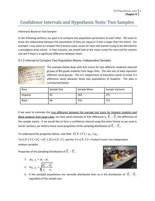
Race Sample Size Sample Mean Sample Variance 

Hispanic 45 264 375 

Black 46 256 372 

If we want to estimate the true difference between the average test score for Hispanic students and 

Black students from large cities, our best point-estimate of that difference is X1 − X 2 the difference of 

the sample means. If we would like to form a confidence interval using the same format as we used in 

earlier sections, we need to know some properties of the sampling distribution of X1 − X 2 . 

To understand the properties below, note that: E ( X ± Y ) = µ X ± µ Y , 

2 2 

Var ( X ± Y ) = σ + σ ± 2 Cov( X , Y ) , and the ( , ) 0 

random variables. 

X Y 

Properties of the Sampling Distribution of X1 − X 2 : 

1. 

2. 

µ = µ − µ 

X1− X2 

1 2 

σ σ 

σ = + 

X1− X 2 n n 

2 2 

1 2 

1 2 

Cov X Y = when X and Y are independent 

X − X 

3. If the sampled populations are normally distributed then so is the distribution of 1 2 

regardless of the sample size. 

1


Chapter 9 

4. If the sampled populations are not normal then we will need to have large sample sizes to 

X − X by the normal distribution. 

ensure that we can approximate the distribution of 1 2 

***Note: We are assuming that the samples drawn are independent. 

2 2 

† † Note: If σ &σ 

are unknown, we may use their sample estimates as approximations as long as 

1 2 

the sample sizes are large (> 30). 

Using the properties above and the same structure as we used in previous sections, we can find a 

formula for the: 

(1-α )100% Confidence Interval for the True Difference Between the Population Means 

(Point Estimator) ± (Number of Standard Deviations)(Standard Error) 

X1 − X 2 ± Zα / 2 

σ σ 

+ 

n n 

2 2 

1 2 

1 2 

* assuming that the two samples are independent. 

To use the above formula we must have large sample sizes ( > 30 ), and the samples must be randomly 

drawn from independent populations. 

Remember, that if we do not know the population standard deviation, but the sample size is large we 

can use the sample estimates. In other words, 

σ σ 

( x1 − x2 ) ± zα / 2 σ ( x1 −x2 

) = ( x1 − x2 ) ± zα 

/ 2 + 

n n 

2 2 

1 2 

1 2 

s s 

≅ ( x1 − x2 ) ± zα 

/ 2 + 

n n 

2 2 

1 2 

1 2 

Now let’s use the above formula we just found on the example below: 

2


Chapter 9 

Example 131: The U.S. Department of Education conducts an assessment of student learning called the 

National Assessment of Educational Progress (NAEP). From the 2009, grade 

8 mathematics assessment random samples were drawn from two groups: 

Hispanic males from large cities and Black males from large cities. The data 

is summarized below. Use the data to form a 95% confidence interval for 

the true mean difference for grade 8, mathematics scores between Hispanic 

males and Black males from large cities. 

Race Sample Size Sample Mean Sample Variance 

Hispanic 45 264 375 

Black 46 256 372 

Steps for constructing the Confidence Interval for the True Difference between the Population Means: 

Step 1 Gather Data from Problem, Calculate X1 − X 2 , and Calculate 

Step 2 Find Zα / 2 

Step 3 Use the results from steps 2 and 1 to get the margin of error, E = Z 

⎡⎣ ( X − X ) − E,( X − X ) + E⎤⎦ 

Step 4 Form 1 2 1 2 

Let’s do that one more time using different data: 

2 2 

σ1 σ 2 + . 

n n 

1 2 

α / 2 

σ σ 

+ 

n n 

2 2 

1 2 

1 2 

3


Chapter 9 

Example 132: Recent studies have indicated that low carbohydrate diets are at least as effective as low 

fat diets in reducing weight. Does it matter which low carbohydrate diet 

is followed? Two samples of overweight, premenopausal women were 

randomly assigned to either the Atkins diet or the Zone diet for one year. 

At no point in the yearlong study was total calorie consumption different 

between the two groups. The results of the study are summarized 

below. Construct the 98% confidence interval for the true difference 

between the weight loss amounts achieved on the two low carbohydrate 

diets. 

Diet Sample Size Sample Mean Sample Standard Dev. 

Atkins 77 10.34 lbs 15.86 lbs 

Zone 79 3.52 lbs 11.74 lbs 

9.2 Z-Test to Compare Two Population Means: Independent Samples 

Next, we will look at the method of testing hypotheses of the form: : ( µ µ ) 

( µ µ ) 

1 2 0 

H − = D vs. 

0 1 2 0 

H : − ≠ D (note: as usual the null hypothesis may have the symbols ≤or≥ , and the 

A 

alternative hypothesis may have > or


Chapter 9 

These are basically the same seven steps that we used to test hypotheses in previous sections; however, 

there are some minor changes that occur in the steps with asterisks by them. For example, the 

hypotheses will look as described above, and we will have a new test statistic, given by: 

z = 

( ) 

X − X − D 

1 2 0 

σ σ 

+ 

n n 

2 2 

1 2 

1 2 

Other important things to consider are the test assumptions, which are as follows: 

1. The samples are randomly selected and independent. 

2. The sample sizes are both > 30. 

Example 133: Tests of the effectiveness of Echinacea in preventing upper respiratory infections in 

children were conducted in double blind studies. “Days of 

Fever” was one criteria used to test the effectiveness of 

Echinacea. Among 337 children treated with Echinacea, 

the mean number of days with fever was 0.81, with a 

standard deviation of 1.5 days. Among 370 children given a 

placebo, the mean number of days of fever was 0.64 with a 

standard deviation of 1.16 days (JAMA Vol. 290). Use a 5% 

significance level to test the claim that Echinacea affects the number of days with fever. What is the pvalue 

for the test? 

Example 134: In a case in Ireland, a class action lawsuit was brought 

against the government alleging age discrimination. The ages of 31 

randomly selected unsuccessful applicants for promotion yielded a 

mean age of 47 and a standard deviation of 7.2 years. The ages of 30 

randomly selected successful applicants yielded an average age of 43.9 

and a standard deviation of 5.9 years. Using a 5% significance level, test 

the claim that the government is discriminating based on age. 

5


Chapter 9 

9.3 t-Interval to Compare Two Population Means: Independent Samples (Equal Variances) 

What happens when the sample sizes are not greater than 30? There are two consequences of this: 

1. We cannot assume approximate normality (solution: We must know the samples are normally 

distributed to start with—actually as long as there are no outliers in the data and there isn’t too 

much of a departure from normality we can still apply this method). 

2. The sample standard deviations may not be reliable estimates of their population counter parts 

(solution: We will need to use the t-distribution). 

In order to use the t-distribution for this problem, we need to decide between two possible approaches. 

The first scenario assumes that the population variances are equal. Assuming the variances are equal 

will allow us to use a random variable that has an exact t-distribution. If we cannot assume this, we may 

use some other approach such as the Welch-Satterthwaite method which allows us to approximate the 

t-distribution. We will look at the Welch-Satterthwaite method in the next section. 

Example 135: The World Anti-Doping Agency funded a study to compare 

the effects of Growth Hormone on body composition and athletic 

performance in women. Among the 16 subjects assigned to the placebo 

group, the mean fat mass change after eight weeks was -2.1 pounds with 

a standard deviation of 1.2 pounds. Among the 17 subjects assigned to 

injections of growth hormone, the mean fat mass change after eight 

weeks -4.4 pounds with a standard deviation of 1.3 pounds. Construct a 95% confidence interval 

estimate of the difference between the mean weight losses for the two diets (assume weight loss is a 

normally distributed random variable and assume the two groups have equal variances). Does it seem 

that growth hormone has an effect on fat mass in women? 

To do the above problem using the t-distribution, we will first assume that the 

two variances are equal. It is then reasonable to pool the two sample 

2 

variances into one sample estimator ofσ 

. We call this estimator the pooled 

2 

sample estimator ofσ 

(notice it is just a weighted average with the degrees 

of freedom as the weights): 

S 

2 

p 

= 

( − 1) + ( −1) 

n s n s 

2 2 

1 1 2 2 

n + n − 2 

1 2 

To form our confidence interval we will follow the following set of steps: 

6

Step 1 Gather Data for the Problem, Calculate X1 − X 2 , and Calculate 

Step 2 Find / 2 

Step 3 Find E = 

tα using n1 + n2 

− 2 as the degrees of freedom 

S S 

2 2 

p p 

α / 2 + 

n1 n2 

t 

⎡⎣ ( X − X ) − E,( X − X ) + E⎤⎦ 


S 

2 

p 

= 


Chapter 9 

( − 1) + ( −1) 

n s n s 

2 2 

1 1 2 2 

n + n − 2 

1 2 

9.4 t-Test to Compare Two Population Means: Independent Samples (Equal Variances) 

Small-Sample Hypothesis Test of: H : ( µ − µ ) = D , H : ( µ − µ ) ≤ D , or : ( µ µ ) 

0 1 2 0 

0 1 2 0 

H − ≥ D 

0 1 2 0 

We will use the same seven steps as always; however, we will need a new t-test statistic. If we assume 

equal variances, the test statistic for these problems will be: 

The equal variance case 

Steps: 

( − ) − ( − 1) + ( −1) 

X X D n s n s 

t = where S = 

1 2 

2 2 

0 2 1 1 2 2 

, 

2 2 

p 

S n1 n2 

2 

p S 

+ − 

p 

+ 

n n 

1 2 

1. Express the original claim symbolically 

2. Identify the Null and Alternative hypothesis 

3. Record the data from the problem 

4. Calculate the test statistic* 

5. Determine your rejection region 

6. Find the initial conclusion 

7. Word your final conclusion 

, and d.f.= n1 + n2 

− 2 

7


Chapter 9 

Example 136: When investigating the link between birth weights and IQ scores, researchers found that 

28 subjects with birth weights less than 1000g had a mean IQ of 95.5 and a 

standard deviation of 16.0. For 27 subjects with normal birth weights, the 

mean IQ was 104.9 with a standard deviation of 14.5. At the 5% significance 

level, test the claim that low birth weight children have lower IQs than 

normal birth weight children (assume IQ scores are normally distributed and 

the variances are equal). Is there a possible problem with the assumption of equal variances here? 

9.5 t-Interval to Compare Two Population Means: Independent Samples (Unequal Variances) 

Example 137: A study was done to determine the effects of a 6-day administration of growth hormone 

on strength gains in men who perform the bench press. Two 

groups of men were randomly selected for the study. Twenty-five 

of them were placed into the (placebo) control group. Twentythree 

of the men were given a six-day dose of growth hormone (19 

mcg/kg/d). On day one of the study strength in the maximum 

bench press was recorded for each subject, and it was shown that 

the two groups were not significantly different from each other at 

that point in the study. Seven days after the last of the growth 

hormone injections were administered, strength in the maximum 

bench press was recorded again. The control group had an average 

max bench of 220 pounds and a standard deviation of 24 pounds. The growth hormone group had an 

average max bench press of 251 pounds with a standard deviation of 18 pounds. Construct a 98% 

confidence interval estimate of the difference between the mean max bench press for the two groups 

(assume maximum bench press is a normally distributed random variable and do not assume equal 

variances). Does there appear to be a significant difference between the strength of the two groups? 

8


Chapter 9 

To do the above problem without assuming equal variances, we will need to use an approximation 

method called the Welch-Satterthwaite method. To do this, let’s modify the traditional four steps: 

Step 1 Gather Data from Problem, Calculate X1 − X 2 , Calculate 

s s 

+ 

n n 

2 2 

1 2 

1 2 

Step 2 Find tα / 2 using the degrees of freedom formula = 

2 

2 

s1 

s2 

A = , Calculate B = , and Calculate 

n 

n 

( ) 2 

A + B 

1 2 

1 

*(truncate to the nearest whole 

2 2 

A B 

+ 

n −1 n −1 

number) Note: if the sample sizes are the same you can use n1 + n2 

− 2 instead of the formula above. 

Step 3 Find E = 

s s 

2 2 

1 2 

α / 2 + 

n1 n2 

t 

⎡⎣ ( X − X ) − E,( X − X ) + E⎤⎦ 


Note: Do not assume equal variances for the small sample size problems unless specified. That means 

you will use the Welch-Satterthwaite method unless the problem says you can assume equal variances. 

Example 137.5 Student loan debt is a concern for many college bound high school seniors. In Miami, the 

two top research schools are Florida International University and the 

University of Miami. A sample of 29 recent graduates from FIU who 

borrowed money for school had an average debt load of $16,026 and 

a standard deviation of $10,738. A sample of 29 recent graduates 

from UM who borrowed money for school had an average debt load 

of $26,438 and a standard deviation of $16,203. Use the data from 

the two randomly selected groups of college graduates to construct a 

99% confidence interval estimate of the true difference between the 

average amount of student loan debt carried by FIU graduates and 

UM graduates. 

2 

9


Chapter 9 

9.6 t-Test to Compare Two Population Means: Independent Samples (Unequal Variances) 

Small-Sample Hypothesis Test of H : ( µ − µ ) = D , H : ( µ − µ ) ≤ D , or : ( µ µ ) 

0 1 2 0 

0 1 2 0 

H − ≥ D 

0 1 2 0 

We will use the same seven steps as always; however, we will need a new t-test statistic. If we assume 

unequal variances, the test statistic for these problems will be: 

The Welch-Satterthwaite method (unequal variance case): 

t = 

( ) 

X − X − D 

1 2 0 

s s 

+ 

n n 

2 2 

1 2 

1 2 

( ) 2 

A + B 

2 

s1 

s 

, where t has degrees of freedom = 

and A = and B = 

2 2 

A B n1 

n 

+ 

n −1 n −1 

1 2 

Note: if the sample sizes are the same you can use n1 + n2 

− 2 instead of the formula above. 

Example 138: When investigating the link between consuming canned foods and bisphenol A (BPA) 

levels in people, researchers found that 26 subjects who ate a can of soup 

everyday for five days had average BPA levels of 20.8 micrograms per liter 

of urine and a standard deviation of 3.1 micrograms per liter. For 27 

subjects who ate fresh soup, their mean levels were 1.1 micrograms per 

liter of urine and a standard deviation of 0.5 micrograms per liter. At the 

5% significance level, test the claim that consuming canned soup raises 

the concentration of BPA in urine (assume BPA levels are normally distributed and do not assume equal 

variances). 

2 

2 

2 

10

Summary flow chart for methods: 


Chapter 9 

9.7 Hypothesis Test to Compare Two Population Means: Matched-Pair Experiments 

Comparing Two Populations Means: Paired Difference Experiments 

Comparing Two Population Means: Matched Pairs 

For large samples where we 

2 2 

do not knowσ or σ , we 

1 2 

2 2 

can use s or s as 

substitutes. 

1 2 

Recall that our goal in the previous section was to be able to detect a difference between two 

population averages. The example problem below requires a similar sort of analysis. We would like to 

11


Chapter 9 

be able to detect if the scores for students taking the FCAT math section improve after completing a 

series of FCAT prep classes. 

Example 139: Below is a table of FCAT SSS developmental scores for a group of students who were 

struggling with math in the 3 rd grade. 

FCAT math scores for 8 struggling students 

Student After Prep Before Prep 

1 290 275 

2 275 270 

3 380 370 

4 260 245 

5 340 325 

6 270 260 

7 280 270 

8 215 200 

We want to test the claim: The prep classes work to improve FCAT math SSS scores. 

(In symbolic form: µ − µ > 0 ) 

After Before 

Using the method from the previous section where we assume the two sets of data are drawn from 

independent populations, we get a test statistic of: t = 0.467, which is not significant. This means we 

cannot reject the null ( µ − µ ≤ 0 ), and we conclude that the prep classes are not effective at 

After Before 

raising FCAT SSS scores. Does that seem correct when we look at the table of values above? Isn’t it true 

that every student improved their math score after attending the prep classes? Then why did we get 

this result? 

The answer is that the method we used is not valid here. In the previous section, our assumption was 

that the two samples were independent, but that is not true here. The two samples above were drawn 

from the same students. We gave them the FCAT, and then we gave them prep classes and retested the 

same students. 

12


Chapter 9 

Okay, so we violated the assumptions—so what? Why does that affect our ability to detect the 

difference between the two FCAT 

performances? The answer lies in the 

quantity: 

S 

2 

p 

= 

( − 1) + ( −1) 

n s n s 

2 2 

1 1 2 2 

n + n − 2 

1 2 

= 2,581.03 This is 

our pooled variance for the t-test we 

constructed above. What is this measuring in 

this case? It is measuring the variation of the 

FCAT scores between the students—not the 

differences between the scores each 

individual earned before and after prep. In 

other words, it is not looking at the difference 

between before and after exams, but rather 

looking at the differences between student 

abilities. We know there are great differences 

between different students’ ability, but that is 

not what we want to look at in this problem. 

How does using the wrong measure of 

variation affect our hypothesis test? 

We are trying to look at the average difference between the before and after FCAT scores. If the test 

prep has no effect, we would expect the average difference of before and after scores to be zero. To 

know if the true difference is significantly different from zero, we will need to consider the variation of 

the differences between before and after FCAT scores. If the average distance between the before and 

after FCAT scores and zero is not much larger than (or is small) compared to the natural variation that 

occurs between retakes of the FCAT, we will conclude there is no significant improvement due to the 

prep classes. 

To help you understand this idea, consider this simple example: Johnny scores a 170 on his FCAT math 

section, and Suzy scores a 460 on her FCAT math section. After taking the prep classes, Johnny retakes 

the FCAT and improves his grade to a 190, while Suzy’s score jumps to a 490. 

What is the difference within each student’s before and after scores? 

Suzy’s score change = 490 – 460 = +30, Johnny’s score change = 190 – 170 = +20 

Average score change = + 25 

13

What is the difference between the students’ scores 

however? 

Before difference = Suzy(460) – Johnny(170) = 290 

After difference = Suzy(490) – Johnny(190) = 300 

Average difference = 295 


Chapter 9 

If you compare these two numbers, it is clear the average within score change is quite small compared 

to the differences between Johnny’s and Suzy’s FCAT scores, but we do not want to compare these two 

quantities do we? No, we would want to compare the average before and after score change against 

the variation of the individual students’ score changes not the variation of the individual test scores 

(that variation is great do to the different math ability of the students). 

We need to find a way to ignore these differences between different students’ FCAT scores. These 

differences are not important to us. In other words, we know Suzy scores higher than Johnny already. 

We want to know if the prep course helps students do better regardless of how they did before. We do 

not want the differences in student ability to obscure the differences between before and after scores 

that we are interested in. If we can’t block out the differences between students, we will never be able 

to detect the smaller differences that are occurring between before and after test scores. It would be 

like trying to hear the footsteps of a mouse running across a concert hall floor while a rock concert is 

being played in the same hall. 

Blocking 

We do have a very simple solution to this problem: we will run a one-sample t-test on the differences 

between before and after scores: 

Subject 1 2 3 4 5 6 7 8 

After 290 275 380 260 340 270 280 215 

Before 275 270 370 245 325 260 270 200 

Just subtract each subject’s after and before scores… 

14

Subject 1 2 3 4 5 6 7 8 

After 290 275 380 260 340 270 280 215 

Before 275 270 370 245 325 260 270 200 

Difference 15 5 10 15 15 10 10 15 


Chapter 9 

Then treat the row of differences as a single sample. We can get the average difference X d = 11.875 , 

the standard deviation for the differences S d = 3.720 , and the number of differences n d = 8 . Then we 

can use the same test statistic we used for a one-sample t-test: 

t 

X 

− µ 

d d = with degrees of freedom = nd − 1 

Sd 

n 

d 

Where do we get µ d ? That is the hypothesized value for the true average difference. This leads us to 

the question, “what will our claims look like?” 

We will be conducting our hypothesis test using the following pair of competing claims: 

H : µ ≤ D 

0 d 0 

H : µ > D * 

A d 

0 

Now let’s finish our example properly: 

*Of course, all the usual null/alternative pairings are possible 

1. Express the original claim symbolically: µ d > 0 * 

H0 

: µ d ≤ 0 

2. Identify the Null and Alternative hypothesis: 

H : µ > 0 

A d 

3. Record the data from the problem: X = 11.875, S = 3.720, n = 8, α = 0.05 

d d d 

X d − µ d 11.875 

4. Calculate the test statistic: t = = ≈ 9.029 

S 3.720 

d 

n 

d 

5. Determine your rejection region: t > 1.895 

6. Find the initial conclusion: Reject the null, support the alternative 

7. Word your final conclusion: The sample data support the claim that the prep classes are 

effective at improving student’s FCAT SSS math scores. 

8 

15


Chapter 9 

*Note: our claim that the prep classes improve scores indicates that theoretically the ‘after’ exam will be 

better than the ‘before’ exam. This means if we form the difference d = After – Before, the differences 

and their average should be positive, i.e. µ d > 0. 

Some other examples where blocking would be necessary: 

• A study of the effect of a Gulf hurricane on gas prices. If we poll stations across the country 

and look at the price of gas before and after the storm at those stations. Since prices vary from 

state to state, region to region, we would want to block out those differences by looking at 

every station twice (once before the storm and once after). 

• A study wants to look at the difference between starting salaries of their male and female 

graduates. Since differences between majors and GPAs could affect salaries we would pair 

male and females in the study who have similar GPAs and majors. Then we would look at the 

differences in their starting offers. 

• A study wants to compare the absorption rates of two different drugs for pain relief. Since 

there are so many possible differences between patients it would be best to make sure every 

study participant takes both drugs one after the other (allowing for the total elimination of the 

drug that was administered first). This will ensure the differences between the patients do not 

obscure the differences in the absorption rates between the drugs. 

Example 140 The drug Depo-Provera is often used for patients who exhibit hypersexual behavior caused 

by traumatic brain injury (TBI). The results of a study conducted on 8 

patients who exhibited such behavior are included below. Each patient 

had their testosterone levels taken before treatment with Depo and 

after treatment. At the 1% significance level, test the claim that the 

drug is effective at reducing testosterone levels in TBI patients. 

Patient 1 2 3 4 5 6 7 8 

Pretreatment 849 903 890 1092 362 900 1006 672 

After Depo 96 41 31 124 46 53 113 174 

Differences 753 862 859 968 316 847 893 498 

Next, we will look at the confidence interval for paired differences data. 

16


Chapter 9 

9.8 Confidence Interval to Compare Two Population Means: Matched-Pair Experiments 

The procedure to construct a confidence interval for data from a Matched-Pair Experiment involves the 

same approach that we used in our earlier work with the hypothesis test. We will first need to find all of 

the before – after differences. 

Confidence Interval for Paired Differences: 

Required assumptions: 

⎡ Sd S ⎤ 

d 

⎢X d − tα / 2 , X d + tα 

/ 2 ⎥ 

⎢⎣ nd nd 

⎥⎦ 

1. We must assume that the sample was chosen randomly from the target population. 

2. We must assume that the population of differences has a normal distribution. 

Steps to Form a Confidence Interval for Matched-Pairs Data: 

Step 1 Use subtraction to create your set of differences and determine , , 

d d d 

level. 

Step 2 Find tα /2 

Step 3 Use the results from steps 2 and 1 to get the margin of error, E = tα 

/2 

Step 4 Form ( X − E, X + E) 

d d 

n X S , and your confidence 

Example 141 Use the data from the Depo-Provera study to form a 98% 

confidence interval for µ d , then interpret the results. Are they consistent 

with the results found in the hypothesis test we conducted? 

s 

d 

n 

d 

17

Example 142 Use the data from the FCAT problem that opened this section to form a 90% confidence 

interval for µ d the true average differe difference between before and after FCAT scores and interpret inter the 

results. 


Chapter 9 

9.9 Inference Procedures to Compare Two Population Proportions: Independent Sampling 

Many times we have a need to answer questions that involve the comparison of two population 

proportions. Consider the example below: 

Example 143: A product reliability study was conducted on laptops by the company Square Trade Inc. 

Among 11,500 entry-level level laptops (priced between $400 - $1000) followed for one year, 541 

malfunctioned. Among 9,300 premium laptops (priced over $1000) followed for one year, 391 

malfunctioned. Use a 0.01 significance level to test the claim that the incidence of mal malfunction mal is higher 

for entry-level laptops than it is for premium laptops. Does es it seem that spending more money on a 

laptop will offer you some protection otection from the inconvenience of a malfunction? 

18


Chapter 9 

To answer this question we need to know what quantities to compare. Let’s look at what we have here: 

Entry-level Premium 

X 541 391 

n 11,500 9,300 

ˆp 0.047 0.042 

Clearly, for this sample, premium laptops had a slightly lower malfunction rate for the first year, but is 

this difference just a coincidence? Maybe this could have happened by chance—after all the there is 

always some random sampling error present. 

What we can do is create a test statistic around the difference between these two sample proportions 

( pˆ pˆ 

) 

− using the standard deviation of the sampling distribution for the difference between these 

1 2 

two sample proportions. Then if the sample sizes are large enough*, we can express the probability that 

we would observe this difference ( pˆ pˆ 

) 

assumption under the null hypothesis). 

− by random chance given that they are really the same (the 

1 2 

*Sample sizes are large enough when ˆ 3 

ˆ ˆ pq 

p ± is entirely captured inside [0, 1]. Another rule of 

n 

thumb that is used is: Samples sizes are large enough if n1 pˆ ˆ 

1 ≥ 15 and n1q1 ≥15 

n pˆ ≥15 and n qˆ 

≥15 

So our point estimator for the true population difference will be: ( pˆ − pˆ 

) 

The standard error of its sampling distribution will be: 

p q p q ⎛ 1 1 ⎞ x + x 

+ ≈ pq ˆ ˆ ⎜ + ⎟, 

where pˆ 

= 

n n ⎝ n n ⎠ n + n 

1 1 2 2 1 2 

1 2 1 2 1 2 

2 2 2 2 

1 2 

19


Chapter 9 

Note: ˆp is considered the pooled estimator of the population proportion under the null’s assumption that 

the two groups have the same proportion. 

Our competing hypotheses will be: H : ( p − p ) ≤ 0 Vs. H ( p p ) 

also) 

Our test statistic will be: 

0 1 2 

( pˆ ˆ 

entry−level − p premium ) x1 + x2 

z ≈ , where pˆ 

= 

⎛ 1 1 ⎞ 

n + n 

pq ˆ ˆ ⎜ + ⎟ 

n n 

⎝ 1 2 ⎠ 

A 

: − > 0 ( = , ≠, ≥ , < are possible 

1 2 

1 2 

Now let us determine if we can support the claim that entry-level laptops malfunction more than 

premium laptops. 

1. Express the original claim symbolically: pentry− level > p premium 


0 

( entry−level premium ) 

( − 

) 

H : p − p ≤ 0 

H : p − p > 0 

A entry level premium 

3. Record the data from the problem: pentry− level = 0.047, p premium 

4. Calculate the test statistic: 

= 0.042, α = 0.01 

( pˆ ˆ entry−level − p premium ) 

z ≈ = 

⎛ 1 1 ⎞ 

pq ˆ ˆ ⎜ + ⎟ 

⎝ n1 n2 

⎠ 

0.005 

≈ 1.73 

⎛ 1 1 ⎞ 

0.0448(0.9552) ⎜ + ⎟ 

⎝11500 9300 ⎠ 

5. Determine your rejection region: Z > 2.326 

6. Find the initial conclusion: Do not reject the null, Do not support the alternative 

7. Word your final conclusion: The sample data does not support the claim that entry-level laptops 

have a greater malfunction rate in the first year of owner ship than premium laptops. 

20


Chapter 9 

Example 144 In 1995, the American Cancer Society randomly sampled 1500 adults of which 555 smoked. 

In 2005, they surveyed 1750 adults and found that 578 of them smoked. At the 5% level of significance 

test the claim that the proportion of smokers in the population decreased over the ten year period. 

What is the p-value for the test? 

Let’s now look at the confidence interval for the difference between two proportions: 

Confidence Interval for( p − p ) : 

1 2 

p q p q pˆ qˆ pˆ qˆ 

p − p ± z + ≈ p − p ± z + 

( ˆ ˆ ) ( ˆ ˆ ) 

1 1 2 2 1 1 2 2 

1 2 α / 2 

n1 n2 1 2 α / 2 

n1 n2 

Steps for constructing the Confidence Interval for the True Difference between the Population 

Proportions (large, independent samples): 

Step 1 Gather Data from Problem, 1 1 1 2 2 2 

Step 2 Find Zα / 2 

n , pˆ , qˆ , n , pˆ , qˆ , and the Confidence level. 

Step 3 Use the results from steps 2 and 1 to get the margin of error, E = 

Step 4 Form ( ˆ ˆ ) , ( ˆ ˆ ) 

⎡ p − p − E p − p + E⎤ 

⎣ 1 2 1 2 ⎦ 

z 

pˆ qˆ pˆ qˆ 

1 1 2 2 

α /2 + 

n1 n2 

21

Example 145 Randy Stinchfield of the University of Minnesota studied 

the gambling activities of public school students in 1992 and 1998 

(Journal of Gambling Studies, Winter 2001). His results are reported 

below. Form a 99% confidence interval to estimate the true difference 

between the proportion of public school students who gambled in 

1992 and 1998. Does there seem to be a difference? 

1992 1998 

Survey n 21,484 23,199 

Number who gambled 4,684 5,313 

Proportion who gambled .218 .229 


Chapter 9 

Example 146 In 1995, the American Cancer Society randomly sampled 1500 adults of which 555 smoked. 

In 2005, they surveyed 1750 adults and found that 578 of them 

smoked. Form a 90% confidence interval for the difference between 

the proportion of smokers in 1995 and 2005. Has the proportion 

decreased over the ten year period? 

Interpreting confidence intervals involving the difference between two population proportions is as easy 

as it was for the differences between two means. If the interval is entirely positive, the first proportion 

in your difference is larger. If the interval is entirely negative, the second proportion in your difference 

is larger, and finally, if the interval contains zero it means we cannot say there is a significant difference 

between the two proportions. 

Consider the set of confidence intervals provided below from the Framingham Heart Study which looked 

at the effects of one's social network on drinking habits: 

22


Chapter 9 

23

9.10 Using the f-table to Find Critical Values 


Chapter 9 

Before we begin the next topic, let’s learn how to use the F table found in the back of most textbooks to 

find critical values. If you are curious about where the F-distribution comes from it is the ratio of two 

chi-square distributions with degrees of freedom ν1 andν 2 , respectively, where each chi-square has first 

been divided by its degrees of freedom. 

We will be working with two independent samples of data in the next section, and we will have a need 

to use the F-distribution. The F-tables, like the Z-table and t-table, are used to find critical values. When 

we use the F tables, there will be two degrees of freedom. The degrees of freedom will be 1 1 n − and 

1 n − for the two sample sizes in the problem. The F-test stat is a fraction, so we will consider one of 

2 

these degrees of freedom to be the numerator degrees of freedom and one to be the denominator 

degrees of freedom. This will depend how we set up the ratio in the given problem. For now let’s just 

assume 1 1 n − is the numerator degree of freedom and 2 1 n − is the denominator’s degree of freedom. 

We will also need an alpha value in each problem. This α value will be the amount of area that will be 

found in the upper tail of our F-distribution beyond our critical value. 

f α 

Example 147 Find the critical value 1 2 

Example 148 Find the critical value 1 2 

n −1, n − 1, = 30,40,0.01 

f α 

n −1, n − 1, = 6,24,0.025 

f 

f 

24


Chapter 9 

9.11 Hypothesis Test to Compare Two Population Variances: Independent Sampling 

Comparing Two Population Variances: Independent Sampling 

There are a lot of situations where we want to know if the populations have the same variances. In fact, 

we just studied hypothesis testing methods for comparing two means from independent populations. In 

that section when the sample sizes were small we needed to assume either that the population 

variances were equal or that they weren’t, but with the test we learn here today, we won’t have to 

assume. At other times, we will actually want to compare the variances of two groups for its own sake 

instead of just performing the test to know if we can go forward with a test of the means. The following 

is an example of the latter type of problem: 

Example 149: Disney is comparing two methods of receiving customers at its City Halls in the Magic 

Kingdom and Disney Land. They are deciding if using one long line 

(used in Disney Land) is better than allowing people to line up in 

separate lines for each teller (used in Magic Kingdom). They 

collected waiting time data (measured in minutes) for both 

locations: 

Disney Land: n = 41, X = 5.15, S = 0.48 

Magic Kingdom: n = 61, X = 5.15, S = 1.23 

Test the claim at the 5% significance level that Disney Land “City Hall” lines have a smaller variance than 

the lines at “City Hall” in Magic Kingdom. 

To compare variances we will use an F-test. The F-distribution is the ratio of two chi-square 

distributions with degrees of freedom ν1 andν 2 , respectively, where each chi-square has first been 

divided by its degrees of freedom. It turns out that if a random variable is normally distributed and has 

population variance 

2 

σ the quantity 

( − ) 

2 

S n 

2 

σ 

1 

~ χn 

2 

−1 

(is chi-squared with degree of freedom n-1). This 

means that if we divide our two sample variances we will get a random variable that has an Fdistribution: 

25

S 

S 

2 

1 

2 

2 

~ F 


Chapter 9 

Note, actually we are forming the ratio of two chi-squared random variables divided by their degrees of 

feedom: 

( −1 

) 

/ ( n −1) 

S n S 

2 2 

1 1 1 

2 1 

2 

σ = σ 

2 2 

2 ( 2 −1 

) 2 

/ ( n 

2 

2 −1) 

2 

= 

2 

S1 

2 

2 

S n S S 

σ 

σ 

~ F 

(Why doesn’t 

Answer: Our null hypothesis will include the assumption that σ = σ ). 

To conduct our test we will use the ratio of our two sample variances: 

2 

1 

σ & 2 

σ stay in the denominators? 

2 

1 

2 

2 

S 

S 

2 

2 

1 ~ F 2 n1 −1, n2 

− 1 

2 

* 

*Because of the way most F-tables are constructed, we will always put the larger sample variance on 

top. One way to do this is to always label the sample with the larger sample variance as representing 

population 1. 

2 

1 

0 2 

σ 2 

Our competing hypotheses will be: H : 1 

σ 

≤ Vs. H A : 1 

σ 

> (= vs. ≠ are also possible). 

σ 

Now let’s work our example: 

1. Express the original claim symbolically: 

variance was the smaller of the two) 


σ 

2 

1 

2 

2 

2 

MagicKingdom 

2 

DisneyLand 

σ 

H 

H 

2 

MagicKingdom 

0 2 

σ DisneyLand 

A 

> 1 (because we claimed Disney Land’s 

σ 

: ≤ 1 

σ 

: > 1 

σ 

2 

MagicKingdom 

2 

DisneyLand 

Disney Land: n = 41, X = 5.15, S = 0.48 

3. Record the data from the problem: 

Magic Kingdom: n = 61, X = 5.15, S = 1.23 

4. Calculate the test statistic: 

( 1.23) 

( ) 

2 

2 

0.48 = 

6.566 

5. Determine your critical value and rejection region: F > 1.64 (see the F-Tables) 

26

Steps to determine the critical value for an F-test: 

a. Determine the number of tails and alpha (divide alpha 

in half if two-tails) 

b. Determine the table to use based on step a. 

c. Use the numerator degree of freedom for the top row 

of table and the denominator degree of freedom for 

the left column of the table. 


Chapter 9 

6. Find the initial conclusion: Reject the null, support the alternative 

7. Word your final conclusion: The sample data support the claim that the waiting times at Disney 

Land have less variance than the waiting times at Magic Kingdom. 

Assumptions for the above test: 

1. The samples are random and independent 

2. Both populations are normally distributed (the test is very sensitive to violations of this 

assumption.) 

Example 150 Coke Versus Pepsi, the weights (in pounds) of samples of 

regular Coke and regular Pepsi have been summarized below. Sample 

statistics are shown. Use the 0.05 significance level to test the claim that 

the weights of regular Coke and the weights of regular Pepsi have the 

same standard deviation. 

Regular Coke Regular Pepsi 

Sample size 36 36 

Mean 0.81682 0.82410 

Standard deviation 0.007507 0.005701 

27


Chapter 9 

2 

σ1 

Confidence Interval for : We won’t form this interval in the course, but it is provided here for your 

2 

σ 

reference. 

L, 

α / 2 

U , α / 2 

2 

A (1 − α) × 100% Confidence Interval for σ / σ 

2 2 2 

⎛ s ⎞⎛ 1 1 ⎞ ⎛ σ ⎞ ⎛ 1 s ⎞⎛ 

1 1 ⎞ 

⎜ 2 ⎟⎜ < < 2 2 

s ⎜ 

⎟ 

2 F ⎟ ⎜ ⎟ ⎜ ⎟⎜ 

⎟ 

U , α / 2 σ 2 s ⎜ 

2 F ⎟ 

⎝ ⎠⎝ ⎠ ⎝ ⎠ ⎝ ⎠⎝ 

L, 

α / 2 ⎠ 

2 2 

1 2 

where F leaves ( α/2)% 

of the distribution in a lower tail 

and F leaves ( α/2)% 

of 

the distribution in an upper tail. 

Degrees of freedom are n −1 

in the numerator and 

n −1 

in the denominator. 

2 

Another way to write the above is: 

⎡ 2 2 

S ⎛ 

1 1 ⎞ S ⎤ 

1 

⎢ 2 ⎜ , F 2 U , / 2 

S ⎜ ⎟ 

α 

2 F ⎟ 

⎥ 

⎢⎣ ⎝ L, 

α / 2 ⎠ S2 

⎥⎦ 

1 

Where FL, α / 2 places alpha/2 area in the upper tail of a 

and FU , α / 2 places alpha/2 area in the upper tail of a 

following relationship, 

f 

1 

n1 −1, n2 

−1,1 −α 

/ 2 

= 

f 

n2 −1, n1 

−1, 

α / 2 

Fn1 −1, n2 

−1 distribution, 

Fn2 −1, n1 

−1 distribution. Note: this comes from the 

28

Confidence Intervals and Hypothesis Tests: Two Samples - Florida ...

You also want an ePaper? Increase the reach of your titles

Delete template?

Save as template?