Lecture Notes CT 4860 Structural Pavement Design Design of ...

Lecture Notes CT 4860
Structural Pavement Design
Design of Flexible Pavements
Prof.dr.ir. A.A.A. Molenaar
Delft, March 2007

Table of contents
Preface 3
1. Introduction 4
2. Major defect types in flexible pavements 5
2.1 Cracking 6
2.2 Deformations 9
2.3 Desintegration and wear 11
3. Early design systems, the CBR method 11
4. AASHTO design method 14
5. Development of mechanistic empirical design methods 25
5.1 Introduction 25
5.2 Stresses in a homogeneous half space 27
5.3 Stresses in two layer systems 32
5.4 Stresses in three layer systems 41
5.5 Stresses due to horizontal loads 47
5.6 Stresses in multilayer systems, available computer programs 51
6. Axle loads, wheel loads and contact pressures 69
6.1 Axle loads 69
6.2 Wheel loads 74
6.3 Contact pressures 75
7. Climatic data 84
7.1 Introduction 84
7.2 Temperature 84
7.3 Moisture 89
8. Asphalt mixtures 94
8.1 Introduction 94
8.2 Mixture stiffness 94
8.3 Fatigue resistance 102
8.4 Resistance to permanent deformation 108
9. Granular materials 111
9.1 Introduction 111
9.2 Estimation of the resilient characteristics of sands and unbound materials 111
9.3 Estimation of the failure characteristics of unbound materials 121
9.4 Allowable stress and strain conditions in granular materials 124
10. Base courses showing self cementation 125
11. Cement and lime treated materials 131
11.1 Introduction 131
11.2 Lime treated soils 132
11.3 Cement treated materials 133
12. Subgrade soils 140
12.1 Introduction 140
12.2 Estimation of the subgrade modulus 140
12.3 Allowable subgrade strain 142
13. Special design considerations 143
13.1 Introduction 143
13.2 Edge effect 143
13.3 Reflective cracking 145
14. Design systems 150
14.1 Introduction 150
14.2 Shell pavement design software 150
14.3 ASCON design system 151
14.4 TRH4 155
References 163
2

Preface
In these lecture notes the design of flexible pavements by means of mechanistic empirical
methods is discussed. What do we mean by mechanistic empirical methods? By mechanistic we
mean that the design methods are based on the analysis of stresses and strains in the pavement
structure due to traffic loads or environmental effects using multi layer theory. In order to be
able to make such analyses, assumptions need to be made on the behaviour of the material. We
can e.g. assume that pavement materials behave linear elastic, isotropic and homogeneous. This
however is a serious simplification of reality because most pavement materials exhibit a stress
dependent, elasto-visco-plastic behaviour.
In any case the calculated stresses and strains are then used as input in a transfer function (e.g.
a fatigue relation) that allows us to calculate how many times a particular tensile strain can occur
before failure occurs. This part of the design method is the empirical part. The reason for this is
that although these transfer functions are usually based on extensive material testing in the
laboratory, most of these tests give a specimen property rather then a material property. In other
words: the material characteristic derived from the test result is dependent on the geometry of
the test as well as the way in which the test was performed. Because of this and because the
significant differences in stress conditions as used in the laboratory and those that occur in
practice, as well as the differences in damage initiation and progression between laboratory
specimens and real pavements, the transfer functions as determined in the laboratory cannot be
applied directly to calculate the number of load repetitions to failure for a specific pavement. This
implies that shift factors need to be applied in order to be able to use the laboratory determined
transfer functions for practical purposes. These shift factors often are of significant magnitude
and are commonly based on matching predicted behavior to observed behavior. This makes them
dependent on the local conditions and type of pavement structure involved and empirical
knowledge is needed to derive and use these shift factors successfully.
All this explains why the current design methods are classified as mechanistic empirical.
In these lecture notes we will concentrate on the use of linear elastic multi layer theory for the
calculation of stresses and strains in pavement structures. It will be assumed that the materials
are isotropic, homogeneous and linear elastic. Ample attention however will also be paid to how
the stress dependent, non linear behaviour of unbound materials can be taken into account.
Furthermore the collection of input needed to make a mechanistic empirical based design will be
discussed extensively.
Great care has been given to the preparation of these notes; some errors however can never be
avoided. It is therefore greatly appreciated if you inform the authors about any typing errors you
may find.
Prof. dr. ir. A.A.A. Molenaar
a.a.a.molenaar@citg.tudelft.nl
3

1. Introduction
These lecture notes are dealing with the design of flexible pavements. Before we start with start
with a discussion on stress and strain analyses in such pavements, we better ask ourselves “what
is a flexible pavement” or “what do we define as being a flexible pavement”. In these notes all
pavements which are not considered to be a cement concrete pavement or a concrete block
(small element) pavement are considered to be a flexible pavement. This implies that also
pavements with a relatively stiff cement treated subbase or base are classified as a flexible
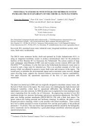
pavement. Some examples of what is considered to be a flexible pavement are given in figure 1.
I
50 mm asphalt
concrete top
layer; 150 mm
unbound base;
150 mm unbound
subbase;
subgrade
SOUTH
AFRICA
II
50 mm asphalt
concrete top
layer; 150 mm
unbound
base; 150 mm
cement treated
subbase;
subgrade
SOUTH
AFRICA
III
50 mm porous
asphalt concrete;
200 mm
asphalt concrete;
300 mm
unbound base of
recycled material;
subgrade
NETHERLANDS
Figure 1: Different types of flexible pavement structures.
IV
200 mm polymer
modified asphalt
concrete; 600 mm
lean concrete
base; subgrade
SCHIPHOL
AIRPORT
AMSTERDAM
In the South African structures, the bearing capacity of the pavement is provided by the unbound
base and subbase (structure I) or by the unbound base and cement treated subbase (structure
II). The asphalt top layer provides a smooth riding surface and provides skid resistance. These
structures have been successfully used in South Africa for moderately (structure I) and heavily
loaded (structure II) roads. The “secrets” of the success of these pavements are the high quality,
4

abundantly available, crushed materials used for the base and subbase and the high levels of
compaction achieved. Furthermore the minimum CBR required for the subgrade is 15%. When
that is not reached, improvement of the subgrade should take place. The cement treated
subbase as used in structure II not only provides a good working platform for the construction
and compaction of the unbound base but also influences the stress conditions in the pavement
such that relatively high horizontal confining stresses develop in the unbound base. As we know
from the lectures on unbound materials (CT4850), unbound materials become stiffer and
stronger when the degree of confinement increases.
Structure III is an example of a highway pavement structure in the Netherlands. One will observe
immediately the striking difference between structure II which is used for heavily loaded
pavements in South Africa and structure III that is used in the Netherlands for these purposes.
The reasons for these differences are quite simple being that the conditions in the Netherlands
are completely different. There are e.g. no quarries in the Netherlands that can provide good
quality crushed materials; these have to be imported from other countries. However, limitations
in space and strict environmental requirements require to recycle materials as much as possible.
Since it has been shown that good quality base courses can be built of mixtures of crushed
concrete and crushed masonry, extensive use is made of unbound base courses made of these
recycled materials. A porous asphalt concrete top layer is used (void content > 20%) for noise
reducing purposes. The thickness of the entire pavement structure is quite significant because
the bearing capacity of the subgrade is quite often not more than 10%. The main reason for the
large thickness however is that the road authorities don’t want to have pavement maintenance
because of lack of bearing capacity. Such maintenance activities involve major reconstruction
which cause, given the very high traffic intensities, great hinder to the road user which is not
considered to be acceptable. For that reason pavement structures are built such that
maintenance is restricted to repair or replacement of the top layer (porous asphalt concrete).
With respect to compaction of the unbound base it should be noted that it would be very hard to
achieve the same results in the Netherlands as in South Africa. In South Africa the excellent
compaction is achieved by soaking the base material and using a high compaction effort. The
excessive amount of water used easily disappears because of the high evaporation rates. The
recycled materials used for base courses in the Netherlands contain a significant amount of soft
material (masonry) which is likely to crush if the compaction effort is too heavy. Furthermore the
excessive amount of water used for compaction will not disappear easily because of the much
lower evaporation rates. Using the South African way of compacting granular base and subbase
courses in the Netherlands will therefore not lead to similar good results.
Structure IV is the structure used for the runways and taxiways of Amsterdam’s Schiphol Airport.
The airport is situated in a polder with poor subgrade conditions (CBR ≈ 2%). Combined with the
airport’s philosophy to maximize the use of the runway and taxiway system and minimize the
need for maintenance, this results in rather thick pavement structures. A total thickness of 200
mm polymer modified asphalt concrete is used to reduce the risk for reflective cracking. For that
reason the lean concrete base is also pre-cracked.
From the discussion given above it becomes clear that the type of pavement structure to be
selected depends on the available materials, climatic conditions, maintenance philosophy etc.
From the examples given above it also becomes clear that one has to be careful in just copying
designs which seem to be effective and successful in other countries. One always has to consider
the local conditions which influence the choice of a particular pavement type.
2. Major defect types in flexible pavements
Pavements are designed such that they provide a safe and comfortable driving surface to the
public. Of course they should be designed and constructed in such a way that they provide this
surface for a long period of time at the lowest possible costs. This implies that the thickness
5

design and the material selection should be such that some major defect types are under control
meaning that they don’t appear too early and that they can be repaired easily if they appear.
Major defect types that can be observed on flexible pavements are:
- cracking,
- deformations,
- disintegration and wear.
A short description of these defect types and their causes is given hereafter. Later in these notes
it will be described how these defect types are taken care of in pavement design.
2.1 Cracking
Cracks in pavements occur because of different reasons. They might be traffic load associated or
might develop because of thermal movements or some other reason. Figure 2 e.g. shows a
combination of wheel track alligator cracking and longitudinal cracking. These cracks are wheel
load associated.
Figure 2: Longitudinal and alligator cracking in the
Wheel path.
Please note that the cracks only appear
in the right hand wheel track close to the
edge of the pavement. This is an
indication that the cracks are most
probably due to edge load conditions
resulting in higher stresses in the wheel
track near the pavement edge than those
that occur in the wheel track close to the
center line. Because of this specific
loading condition, cracks might have
been initiated at the top of the
pavement.
Figure 3 is a picture of a cracked surface
of a rather narrow pavement. If vehicles
have to pass each other, the outer
wheels have to travel through the verge.
From the edge damage that is observed
one can conclude that this is regularly
the case. The base material which is
visible in the verge seems to be a stiff
and hard material. This is an indication
that some kind of slag that shows self
cementing properties was used as base
material. Further indications of the fact
that such a base material has been used
can be found from the fact that the
pavement surface is smooth; no rutting
is observed. The extensive cracking of
the pavement surface might be a
combination of shrinkage cracks that
have developed in the base. It is
however also very well possible that the
adhesion between the asphalt layer and
the base is rather poor. If this is the case
then high tensile strains will develop at
the bottom of the asphalt layer causing
this layer to crack.
6

Figure 3: Cracking observed on a narrow
polder road in the Netherlands.
Figure 4: Low temperature cracking observed on
a highway in Minnesota.
Figure 4 is a typical example of low
temperature cracking. In areas with
cold winters, this type of cracking is
quite often the dominating cracking
type. Due to the very cold weather, the
asphalt concrete wants to shrink. In
principle this is not possible and tensile
stresses develop as a result of the drop
in temperature. The magnitude of the
tensile stress depends on the rate of
cooling and the type of asphalt
mixture; especially the rheological
properties of the bituminous binder are
of importance. If the tensile stresses
are becoming too high, the pavement
will crack at its weakest point. Further
cooling down of the pavement results
in additional cracking and existing
cracks will open. It is obvious that
crack spacing and crack width are
interrelated. A large crack spacing
results in wide cracks and vice versa.
Low temperature cracking can be the
result of a single cooling down cycle
but also can be the result of repeated
cooling down cyclces (low temperature
fatigue).
Figure 5 is an example of temperature
related block cracking. The pavement
of course not only shrinks in the
longitudinal direction but also in the
transversal direction. In that case the
friction between the asphalt layer and
the base is of importance. If that is
high, high tensile stresses might occur
in the transversal direction causing
longitudinal cracks. Combined with the
crack pattern shown in figure 4, this
results in block cracking.
7

Figure 5: Low temperature associated block
cracking observed on a highway in
Minnesota.
As mentioned before, low temperature
cracking can be the major cause of maintenance
and traffic associated cracking is
only of secondary importance in such
cases. However, when heavy wheel loads
are passing a crack like the one shown in
figure 4, high tensile stresses will
develop at the crack edge simply
because of the fact that there is no load
transfer. This problem might increase
during the spring when moisture enters
the crack and weakens the supporting
layers. All this means that although
traffic associated cracking is not the main
problem, traffic can cause accelerated
damage development near cracks.
A type of cracking that has many similarities with low temperature cracking is reflective cracking.
In that particular case, a crack or joint in the layer underneath the asphalt layer tends to
propagate through the asphalt layer. The problem often occurs in pavements with a cement
treated base or overlaid jointed concrete pavements (figure 6). Reflective cracking can even
occur in new pavements when the cemented base shrinks due to hardening. Shrinkages cracks
that develop in the base can easily reflect through the asphalt top layer especially if this layer is
thin. If however the cement treated base is pre-cracked or if shrinkage joints have been made,
the problem of reflective cracking can be minimized.
Figure 6: Example of
reflective cracking in an
overlaid jointed concrete
pavement.
In these lecture notes we will concentrate on traffic induced cracking as well as reflective
cracking. Low temperature is not considered because it is not really an issue in the Netherlands
with its moderate climate.
Of course cracks can develop for many other reasons then traffic and environmental effects. One
example of such “another reason” is given in figure 7 which shows severe cracking in the
emergency lane due to the widening of the embankment next to that lane. Due to the widening,
excessive shear stresses developed in the existing embankment resulting in the development of a
shear plane leading to severe longitudinal cracking not only in the emergency lane but also in the
slow lane (this lane is already repaired as the picture shows). The problem was aggravated by
8

Figure 7: Severe longitudinal cracking due to shear failure in the existing embankment as a
result of widening the road (extended embankment is on the right had side).
2.2 Deformations
Deformations in pavements can be divided in longitudinal and transverse deformations.
Longitudinal deformations can further by divided in short, medium and long wave deformations.
Short wave deformations are of the order of a few centimeters and are mainly caused by surface
irregularities such as raveling (this will be discussed later). Medium wave deformations are in the
order of a few decimeters and usually are caused by imperfections in the pavement structure
itself. Long wave deformations are in the order of meters and are caused by settlements,
swelling soils, frost heave etc. Although they cause major annoyance, long wave deformations
are, because of their origin, outside the scope of these lecture notes.
Figure 8: Roughness due to severe cracking.
the fact that a significant height difference
occurred across the longitudinal crack
resulting in very dangerous driving conditions
for motor cyclists. This type of cracking is
clearly due to a soil mechanics problem and
therefore is beyond the scope of these
lecture notes.
Therefore we will restrict ourselves to short and
medium wave length longitudinal deformations,
also called unevenness or roughness.
Figure 8 shows a severely cracked farm to market
road in Ohio. Due to the extensive amount of
cracking, the pavement has become rather
rough. It is quite clear from the picture that
cracking has not only resulted in longitudinal but
also transverse deformations. It is a typical
example of medium wavelength roughness.
Figure 9 shows a pavement in Zimbabwe. Lack of
maintenance has resulted in potholes which obviously
result in a large decrease of driving comfort.
Even dangerous situations might occur
when driving at night. The reason for the potholes
is that pavement has cracked severely,
comparable to a condition shown in figure 8, and
at given moment small pieces of the surface
layer have been driven out. Erosion of the potholes
due to rain and wind results in depressions
of significant size and depth.
Figure 9: Roughness due to potholes as a result
of severe cracking.
9

Figure 10: Longitudinal deformations due to
settlements.
Figure 11: Rutting in an asphalt pavement.
Figure 12: Unevenness due to “buckling” of
the base made of blast furnace slag.
Figure 10 was taken on a provincial road
close to the Delft University in the
Netherlands. The long wave longitudinal
unevenness that can be observed is clearly
the result of settlements. Please note that
the settlements also have caused deformations
in the transverse direction.
Next to longitudinal deformations, transversal
deformations can occur. These can be the
result of movement of the subsoil (settlements,
swell, frost heave), but they also
might be the result of traffic. The best known
transversal deformation type due to traffic is
rutting or permanent deformation that occurs
in the wheel paths. A typical example of
rutting is shown in figure 11. Rutting can
develop in the asphalt layer(s) or in the
unbound base, subbase or subgrade. Rutting
can be the result of a densification process or
as a result of shear failure. The rutting
shown in figure 11 is clearly caused by shear
failure in the asphalt layer. Shear failure can
be recognized by the ridges that have developed
next to the depression. Furthermore
one can state that the narrower the depresssion
the higher the layer is located in the
structure where the shear failure has developed.
The same is true for corrugations or
washboard formation that is quite often observed
near traffic lights or on unsurfaced
roads.
Figure 12 shows a type of longitudinal unevenness
that is quite often observed on
pavements with a base course made of blast
furnace slags. Because of the chemical
reactions that take place, the material wants
to expand resulting into compressive stresses
that at a given moment become higher than
the compressive strength of the material.
Buckling of the base course is then the result
leading to ridges which negatively influence
driving comfort and which might have a
negative effect on traffic safety because of
loss of cargo from trucks.
10

2.3 Desintegration and wear
Raveling, bleeding and pothole formation can be rated as signs of disintegration and wear.
Pothole formation has already been discussed in the previous section so we will concentrate
ourselves in this section on raveling and bleeding.
Bleeding is a defect type that can be recognized as black, “fatty” looking spots on the pavement
surface. It is an indication of overfilling of the voids in the aggregate skeleton with bituminous
mortar. It is an indication that the mixture is not well designed. Due to the high bitumen content,
the mixture suffers probably from lack of stability at higher temperatures and high traffic loads
might squeeze out the bituminous mortar. Another reason might be that because of the low void
content, there is not enough space for the bituminous mortar when it expands with increasing
temperatures. In any case, the result is the same being a black, shiny surface with hardly any
macro or micro texture and thus a low skid resistance.
Raveling is the loss of aggregate from the surface layer. It can occur on any type of asphalt
mixture but especially open graded mixtures like porous asphalt concrete (void content > 20%)
are sensitive for this damage type (figure 13). Raveling develops because of cohesive failure in
the bituminous mortar or adhesive failure in the interface between aggregate and bituminous
mortar.
Figure 13: Raveling in porous asphalt
concrete.
Note: some aggregate particles are “naked” without any
mortar bonded to the aggregate surface.
Raveling provides a rough pavement surface resulting in an increased noise level. Furthermore
the loose aggregate particles might result in windscreen damage. If raveling occurs on
pavements with a thin asphalt surfacing, like the one shown in figure 9, it might be the first
indication of pothole formation.
3. Early design systems, the CBR method
Until now we have discussed damage types that can occur on flexible pavements. Before we start
discussing the mechanistic empirical design systems that are developed, some information on the
early design systems is given. Some knowledge on these systems is necessary because they are
still used in several parts of the world and because it gives an understanding on how and why
design systems developed to the mechanistic empirical systems used nowadays. Figure 14 is an
11

example of the problems one encountered in the early years of motorization. In those days most
roads were earth or gravel roads and the strength of the pavement solely depended on the shear
strength of the materials used.
Figure 14: Pavement problem in the
early years of motorization.
One has to realize that nowadays about 65% of the global road network still consists of earth
and gravel roads. Problems as shown in figure 14 therefore still quite often occur as is shown in
figure 15.
Figure 15: Timber truck completely
stuck on an earth road due to too
high contact pressures and a too low
shear resistance of the pavement
material.
In both cases it is clear that the stresses induced in the pavement are higher than the allowable
ones resulting in shear failure of the pavement surface and resulting in the fact that in both cases
the vehicle got “stuck in the mud”. The question now is why a light vehicle, such as shown in
figure 14, suffered from the same problems as the heavy vehicle shown in figure 15. This has to
do with the fact that the contact pressures caused by the light vehicle shown in figure 14 are of
the same order of magnitude as the contact pressures caused by the heavy vehicle shown in
figure 15. The lesson we learn from this is that it is not really the weight of the vehicle that is of
importance or the number of axles but the contact pressure distribution under the tires. This
distribution not only depends on the wheel load but also on the area over which the wheel load is
distributed. This depends to a very large extent on the tire pressure. In the old days, solid tires
were initially used and when pneumatic tires were introduced, high tire pressures had to be used
because of the size of the tire (see figure 14). This resulted in small contact areas and high
contact pressures (as comparison: the contact pressure under the tire of a race bicycle is high
because these tires are inflated to 700 kPa pressure; the contact area is also small). All this
means that the contact pressure due to the vehicle shown in figure 14 could very well be the
same as the contact pressure due to the vehicle shown in figure 15. Therefore similar types of
surface defects can be expected.
12

The other reason why both vehicles run into problems is the lack of bearing capacity of the
pavement material. On both pictures we notice an excessive amount of water and from our
lectures in soil mechanics we know that an excessive amount of water results in a low shear
resistance especially in case of soils which contain a high amount of fine grained materials. We all
know that the undrained shear strength of a saturated clay or silt is very low. In that case the
cohesion is low and the angle of internal friction is about zero.
From this example it is clear that precise knowledge on the pressures applied to the pavement
and the strength of the materials used is essential in order to be able to design pavements that
can sustain millions of load repetitions.
The early design systems were, not surprisingly, based on determining the required thickness of
good quality layers on top of the subgrade to prevent shear failure to occur in the subgrade. Of
course the required thickness was dependent on the shear resistance of the subgrade and the
amount of traffic. Furthermore the quality of the covering layers had to be such that shear failure
didn’t occur in these layers. This was the basis for the CBR thickness design method which is
schematically shown in figure 16.
In the CBR design charts, the traffic load was characterized by means of a number of commercial
vehicles per day and the shear resistance of the materials was characterized by means of their
CBR value. The charts were used in the following way. First of all the number of commercial
vehicles had to be determined. When this number was known, the appropriate curve had to be
selected. Next the CBR value of the subgrade needed to be determined and the required layer
thickness on top of the subgrade could be estimated by means of figure 16; this will be illustrated
by means of an example. If e.g. the subgrade CBR is equal to α %, then the total thickness on
top of the subgrade of a better quality material should be H1. If the CBR of the base material (for
reasons of simplicity no subbase is applied in this case) is equal to β, then the thickness of a
better quality material (better than the base material) on top of the base should be H2. In most
cases such a material would be asphalt concrete so H2 would be equal to the required asphalt
thickness. The thickness of the base is then H1 – H2.
Thickness
H1
α β
H2 log CBRsubgrade
Increasing amount of traffic
Figure 16: Principle of the CBR design charts.
13

The minimum asphalt thickness to be applied was 50 mm. The CBR values of the unbound
materials used in the pavement structure is determined by means of the CBR test which is
schematically shown in figure 17. Although the test has been described in detail in the part I of
the lecture notes CT4850, a summary of the basics of the test will be given here.
In the CBR test a plunger is pushed into the soil sample with a specific displacement rate and the
load that is needed to obtain that displacement rate is monitored. The load – displacement curve
that is obtained in this way is compared to the load – displacement curve of a reference material
and the CBR is calculated as shown in figure 18.
The CBR design method results in thin asphalt layers which are mainly needed to provide a
smooth driving surface and sufficient skid resistance.
4. AASHTO design method
In the late 1950’s, it was understood that, with the rapid increase in number and weight of the
vehicles, these simple systems were not good enough anymore for the design of pavements and
a strong need for improved methods developed. For that reason the American State Highway and
Transportation Officials (AASHTO) launched a large research program that had to result in a
better understanding of pavement performance in general and in a system that would allow
durable and economical feasible pavement structures to be designed. For that reason a number
of flexible and rigid pavement test sections were built which were subjected to a variety of traffic
loads. This test is known as the AASHO Road Test, the results of which, e.g. the load equivalency
concept, are still used today.
Figure 17: Principle of the CBR test.
14

Fr
Fm
load
Figure 18: Assessment of the CBR value.
It is beyond the scope of these lecture notes to discuss the Road Test in detail. The interested
reader is referred to reference [1].
We will limit ourselves to a short description of the Interim Design Guide published in the early
1980’s [2]. It is important to understand the principles of this guide since it is still being used in
many places all around the world.
One of the most important concepts that was developed during the test was the present
serviceability index (PSI). This index is a number that reflects the “service” that is given by the
pavement to the road user. The index was developed by correlating the physical condition of the
various test sections in terms of the amount of cracking, rutting and unevenness to the ratings
given by a panel of road users to the “service” provided by the pavement to the user. This latter
rating was a number ranging from 5, being very good, to 0, being very poor. For main roads a
PSI level of 2.5 was considered to be minimum acceptable level. The PSI is calculated as follows:
PSI = 5.03 – 1.91 log ( 1 + SV ) – 1.38 RD 2 - 0.01 √( C + P )
Where: PSI = serviceability index,
SV = slope variance, a measure of the unevenness of the pavement surface,
C + P = percentage of cracked and patched pavement surface,
RD = rut depth.
As one could expect, the unevenness of the pavement has a significant effect on the PSI value; it
dominates all the other factors. Detailed analyses of the data however showed that the amount
of cracking and the slope variance correlate well with each other.
The pavement design method that was developed using the results of the AASHO Road Test
involves the calculation of the so called structural number in relation to the allowable drop in PSI
and the number of load repetitions after which this drop in PSI is allowed to occur. The structural
number SN is calculated using:
SN = a1D1 + a2D2 + a3D3
0.1 inch
reference
material
CBR = Fm / Fr * 100%
material as
tested
displacement
15

Where: ai
= structural coefficient of layer i [-],
Di = thickness of layer i [inch],
i = 1 is the asphalt layer, 2 = base, 3 = subbase.
Other factors that are taken into account are the effective resilient modulus of the subgrade.
Furthermore the method allows to design pavements with a certain level of reliability. Also the
variation that occurs in the prediction of the occurring number of load repetitions as well as the
variation that occurs in the layer thickness, structural layer coefficient and subgrade modulus can
be taken into account by means of the overall standard deviation.
The design chart is shown in figure 19.
The subgrade modulus might vary during the year due to seasonal variations. One therefore has
to determine the effective roadbed resilient modulus which is determined using the chart given in
figure 20. Figure 20 is used as follows. One first determines the modulus which is to be used in a
particular month (please note that it also possible to define the subgrade modulus each half
month). Then the relative damage is determined using the scale at the right hand part of the
figure. Next to that the sum is determined of the damage factors and divided by 12 (or 24 if the
damage factor is defined per half month). This value is then used to determine the effective
roadbed or subgrade modulus. An example of how to use the chart is given in table 1.
Month Roadbed soil modulus [psi] Relative damage uf
January 20,000 0.01
February 20,000 0.01
March 2,500 1.51
April 4,000 0.51
May 4,000 0.51
June 7,000 0.13
July 7,000 0.13
August 7,000 0.13
September 7,000 0.13
October 7,000 0.13
November 4,000 0.51
December 20,000 0.01
Average uf 3.72 / 12 = 0.31
Table 1: Calculation of the mean relative damage factor for the estimation of the effective
subgrade modulus.
Since the mean relative damage factor = 0.31, we determine from figure 20 that the mean
effective roadbed (or subgrade) modulus is 5,000 psi.
16

Figure 19: AASHTO design chart for flexible pavements based on using mean values for each
input.
17

Figure 20: Chart to determine the effective roadbed (subgrade) modulus.
18

Charts to determine the structural layer coefficients for asphalt concrete, base and subbase are
given in figures 21, 22 and 23.
The charts given in figures 22 and 23 are based on the following equations:
For the base: a2 = 0.249 log EBS - 0.977
For the subbase: a3 = 0.227 log ESB – 0.839
Both the resilient modulus of the base, EBS, and the subbase, ESB, are stress dependent following
E = k1 θ k2
Figure 21: Chart for determining the structural layer coefficient for asphalt; please
note that the asphalt modulus is at 68 0 F (20 0 C).
Where: E = modulus [psi],
θ = sum of the principal stresses [psi] (see table 2).
k1, k2 = material constants (see table 3).
The sum of the principal stresses in the base and subbase depends of course on the thickness
and stiffness of the layers placed on top of them as well as on the magnitude of the load.
Suggested values for θ are presented in table 2.
As one will notice from table 3, the material constants k1 and k2 are dependent on the moisture
condition of the material (dry, damp, wet) as well as the quality of the material (indicated by the
range in values.
19

Roadbed resilient modulus [psi]
Asphalt concrete thickness [inch] 3000 7500 15000
< 2 20 25 30
2 – 4 10 15 20
4 – 6 5 10 15
> 6 5 5 5
Table 3: Values for k1 and k2 for base and subbase materials.
Also charts have been provided for cement treated bases and bituminous treated base courses.
These charts are shown in figures 24 and 25.
The traffic load is expressed as number of equivalent 18 kip (82 kN) single axles. To get this
number the following equation is used.
Neq = i=1Σ i=n (Li / 82) 4
Where: Neq
= number of equivalent 18 kip (82 kN) single axles,
n = number of axle load classes,
= axle load of axle load class i.
Li
Table 2: Estimated values for θ in the base and subbase.
The reliability level to be used depends on the importance of the road. Freeways and very
important highways are to be designed with a high level of reliability (90% and higher) because
of the fact that traffic delays due to maintenance because of premature failure is not considered
acceptable. Roads of minor importance can be designed with a much lower reliability level. Low
volume roads e.g. can be designed with a reliability level of 60 – 70%.
The overall standard deviation is much more difficult to estimate. It appeared that this value was
0.45 for the asphalt pavements of the AASHO Road Test. Because production and laying
techniques have significantly be improved since then, a lower value could be adopted. Since it is
difficult to estimate a proper value, use of the 0.45 value is still suggested.
20

Figure 22: Chart to estimate the structural layer coefficient for granular
base courses.
21

Figure 23: Chart to estimate the structural layer coefficient for granular
subbases.
22

Figure 24: Chart to estimate the structural layer coefficient of cement treated base
layers.
23

Figure 25: Chart to estimate the structural layer coefficient for bituminous treated
base courses.
Drainage is a very important feature of pavement structures. Insufficient drainage might result in
moisture conditions close to saturation. As we have seen in table 3, such conditions result in
significant lower values for k1 implying that the modulus of the unbound base and subbase can
be 3 times lower in wet conditions than when they are dry. In order to be able to take care for
improper drainage, it is suggested to multiply the structural layer coefficients with a drainage
factor (mi) following:
SN = a1D1 + m2a2D2 + m3a3D3
Recommended m values are given in table 4.
It should be noted that the selection of the actual layer thicknesses has to follow a certain
procedure. First of all one should determine the SN of the entire structure. Following the example
in figure 20, we determine that the required SN = 5. Then we determine the required SN1 on top
of the base. Assuming a modulus of 30000 psi for the base (a2 = 0.14) we determine that SN1 =
2.6 and we determine the required asphalt thickness (assuming a1 = 0.4) as D1 = SN1 / a1 = 2.6
/ 0.4 = 6.5 inch. If we assume that the modulus of the subbase is 15000 psi (a3 = 0.11), we
24

determine in the same way the required thickness on top of the subbase as SN2 = 3.4 The
required base thickness is D2 = (SN2 – SN1) / a2 = (3.4 – 2.6) / 0.14 = 5.8 inch. Furthermore we
calculate the thickness of the subbase as D3 = (SN3 – SN2) / a3 = (5 – 3.4) / 0.11 = 14.6 inch.
Table 4: Drainage factor m.
5. Development of mechanistic empirical design
methods
5.1 Introduction
Although the AASHTO design method was a major step forward it still had the drawback of being
highly empirical. The method in fact is nothing less than a set of regression equations which are
valid for the specific conditions (climate, traffic, materials etc.) of the Road Test. This implies that
it is a bit risky to use the method in tropical countries where the conditions are completely
different. Fortunately, road constructions are forgiving structures implying that the method at
least results in an initial design that can be refined to meet local conditions.
The fact that the AASHTO method cannot be directly used for conditions for which it hasn’t been
developed became very apparent when attempts were made to use it in developing countries.
The main problem was the PSI concept; it appeared e.g. that a pavement in the developed world
with a low PSI implying that immediate maintenance was needed, was still a pavement with an
acceptable quality in developing countries. This clearly indicated the need to have performance
criteria and design methods that fit the needs and circumstances in developing countries. All this
resulted in the development of the Highway Design Model [3], a design system that is fully suited
for those conditions. It is however beyond the scope of these lecture notes to discuss this model
in detail.
Another problem with the Guide is that it gives no information why materials and structures
behave like they do. Furthermore the Guide provides no information with respect to maintenance
that is needed from a preservation point of view. The PSI value e.g. is strongly dependent on
pavement roughness and damage types like cracking and rutting don’t seem to have a large
influence on the PSI. However control of cracking and rutting is important from a preservation
point of view and in order to be able to make estimates on such maintenance needs, knowledge
on stresses and strains and strength of materials is essential. Furthermore, if such information is
not available, then it is almost impossible to evaluate the potential benefits of new types of
materials and structures with which no experience has been obtained yet.
25

Given these drawbacks, one realized immediately after the Road Test that mechanistic based
design tools were needed to support the AASHTO Guide designs. For that reason, much work has
been done in the 1960’s on the analysis of stresses and strains in layered pavement systems [6,
7, 8, 9] and on the characterization of the stiffness, fatigue and permanent deformation
characteristics of bound and unbound pavement materials. The work done on the analysis of
stresses and strains in pavements is all based on early developments by Boussinesq [4] and
Burmister [5]. References [10, 11 and 12] are excellent sources with respect to research on
pavement modeling and material characterization done in those days and should be on the
reading list of any student in pavement engineering. It is remarkable to see that much of the
material presented then still is of high value today.
Since then, much progress has been made and the reader is referred e.g. to the proceedings of
the conferences organized by the International Society of Asphalt Pavements, the proceedings of
the Association of Asphalt Pavement Technologists, the Research Records of the Transportation
Research Board, the proceedings of RILEM conferences on asphalt materials, the proceedings of
the International Conferences on the Bearing Capacity of Roads and Airfields and those of many
other international conferences to get informed about these developments.
Given the possibilities we have nowadays with respect to material testing, characterization and
modeling, it is possible to model pavements structures as accurate as possible using non linear
elasto-visco-plastic models and using advanced finite element techniques that allow damage
initiation and progression to be taken into account as well as the effects of stress re-distribution
as a result of that. Also such methods allow the effects of joints, cracks and other geometry
related issues to be taken into account. Furthermore these methods also allow to analyze the
effects of moving loads which implies that inertia and damping effects can be taken into account.
The question however is to what extent such advanced methods should be used for solving day
to day problems. This is a relevant question because advanced pavement design methods involve
advanced testing and analyses techniques which require specific hardware and skills.
Furthermore pavement design is to some extent still an empirical effort because many input
parameters cannot be predicted with sufficient accuracy on before hand. Examples of such input
parameters are climate, traffic and the quality of the materials as laid and the variation therein.
All this means that although advanced methods provide a much better insight in why pavements
behave like they do, one should realize that even with the most advanced methods one only can
achieve a good estimate of e.g. pavement performance. Obtaining an accurate prediction is still
impossible. Because of this, practice is very much interested in design methods which are, on
one hand, based on sound theoretical principles but, on the other hand, are very user friendly
and require only a limited amount of testing in order to save money and time.
One should realize that the need to use accurate modeling is influenced to a very large extent by
the type of contracts used for road construction projects. In recipe type contracts, the contractor
is only responsible for producing and laying mixtures in the way as prescribed by the client. In
this case the contractor is neither responsible for the mixture design nor the design of the
pavement structure; these are the responsibilities of the client. This immediately implies that the
clients in this case will choose “proven” designs and materials, in other words he will rely on
experience, and the contractor has no incentive to spend much effort and resources in advanced
material research and pavement design methods. If however contractors are made more
responsible for what they make, meaning that contractors take over from the authorities the
responsibility for the performance of the road over a certain period of time, then they are much
more willing to use more advanced ways of material testing and pavement design.
The purpose of these lecture notes is not to provide an overall picture of existing mechanistic
empirical design methods. The goal of these notes is to provide an introduction into pavement
design using the analytical methods and material characterization procedures as they are
common practice nowadays in the Netherlands. This implies that we will concentrate in these
notes on the use of multi layer linear elastic systems and the material characterization needed to
26

use these systems. Also attention will be paid to how to deal with pavement design in case the
main body of the structure consists of unbound materials which exhibit a stress dependent
behaviour. Also the characterization of lime and cement treated layers will be discussed.
5.2 Stresses in a homogeneous half space
Although pavement structures are layered structures, we start with a discussion of the stresses in
a homogeneous half space. Solutions for this were first provided by Boussinesq at the end of the
1800’s. Originally Boussinesq developed his equations for a point load but later on the equations
were extended for circular wheel loads. The stresses under the center of the wheel load can be
calculated using:
σz = p [ -1 + z 3 / (a 2 + z 2 ) 3/2 ]
σr = σt = [ -(1 + 2ν) + 2.z.(1 + ν) / √(a 2 + z 2 ) – { z / √(a 2 + z 2 ) } 3 ] . p / 2
w = 2.p.a.(1 - ν 2 ) / E
Where: σz = vertical stress,
σr = radial stress,
σt = tangential stress,
ν = Poisson’s ratio,
E = elastic modulus,
a = radius of the loading area,
p = contact pressure,
z = depth below the surface.
Please note that the cylindrical coordinate system is used for the formulation of the stresses (see
figure 26).
This is not the place to give the derivations that resulted in the equations given above. The
interested reader is referred to [4, 6].
In figure 27 some graphical solutions are provided for the Boussinesq equations.
The Boussinesq equations are useful to estimate stresses in e.g. earth roads where the road
structure is built by using the natural available material. One can e.g. derive the Mohr’s circles
from the calculated stresses and then one can determine whether the stresses that occur are
close to the Mohr – Coulomb failure line, implying early failure, or not.
Many of these earth roads however are layered systems simply because the top 200 mm or so
have different characteristics than the original material simply because of compaction that is
applied etc. The higher stiffness of this top layer results in a better spreading of the load. This is
schematically shown in figure 28.
27

Figure 26: Cartesian and cylindrical coordinate system.
28

Figure 27: Graphical solutions for Boussinesq’s equations.
29

Figure 28: Effect of applying a stiffer top layer on the spreading of the load.
In order to be able to calculate stresses in such two layered systems, Odemark’s equivalency
theory [13] is of help. The idea behind Odemark’s theory is that the vertical stresses at the
interface between the top layer with stiffness E1 and thickness h1 and the half space with
stiffness Em are the same as the stresses at an equivalent depth heq with stiffness Em. This
principle is shown in figure 29.
Figure 29: Principle of Odemark’s equivalency theory.
The figure shows on the left hand side the distribution of the vertical stresses in a two layer
system. On the right hand side the equivalent heq is shown resulting in the same vertical stress (B)
at the interface between the top layer and the underlying half space.
Odemark showed that the equivalent layer thickness can be calculated using:
heq = n h1 (E1 / Em) 0.33
Em
A
B E1
Em
h1
Em
B
A
Em
E1
heq
Em
30

If Poisson’s ratio of the top layer equals Poisson’s ratio of the half space, then n = 0.9.
The question of course is how well this Odemark/Boussinesq approach allows accurate
predictions of the vertical stresses in pavements to be made. As is shown in figure 30 [14], this
approach seems to be fairly effective in case one is dealing with pavements having unbound
bases and subbases.
Figure 30: Comparison of measured and calculated vertical stresses in pavements.
Let us illustrate the procedure by means of an example. We want to know the stresses in a
homogeneous half space (modulus 100 MPa) that is loaded with a wheel load of 50 kN. Since the
contact pressure is known to be 700 kPa, we can calculate the radius of the loading area
following:
π p a 2 = Q
Where: p = contact pressure,
a = radius of the contact area,
Q = wheel load.
In this way we calculate a = 150 mm. If we assume Poisson’s ratio to be 0.25, then we can
derive from figure 27 that the vertical stress under the centre of the load at a depth of 150 mm
(z = a) is to 60% of p being 420 kPa. Assume that this stress is too high and that a layer is
placed on top of the half space having a modulus of 300 MPa and a thickness of 150 mm. The
equivalent layer thickness of this layer is:
31

heq = 0.9 h1 (E1 / Em) 0.33 = 0.9 * 150 * (300 / 100) 0.33 = 194 mm
We can now calculate the vertical stress using the same Boussinesq chart but this time the depth
at which we have to determine the stress is 194 + 150 = 344 mm which is at a depth of z = 2.3
a.
From figure 27 we notice that now the vertical stress is equal to approximately 20% of p being
140 kPa.
5.3 Stresses in two layer systems
If the stresses in the subgrade, the half space, due to the wheel load are too high, a stiff top is
needed to reduce these stresses. Such a system, a stiffer layer on top of a softer half space, is
called a two layer system. It could represent e.g. a full depth asphalt pavement on top of a sand
subgrade.
Burmister [5] was the first one who provided solutions for stresses in a two layer system. Again,
it is beyond the scope of these lecture notes to provide a detailed discussions on the mathematical
background. Here only attention will be paid to the results of those mathematical analyses
and how they can be used in practice.
Figure 31 shows the effect of a stiff top layer on the distribution of the vertical stresses in a two
layer system. First of all we notice that the distribution of the vertical stress is bell shaped.
Furthermore we notice that the magnitude of the vertical stress is quite influenced by the
stiffness of the top layer. The width of the stress bell however is much less influenced by the
stiffness of the top layer.
Figure 31: Distribution of the vertical stress in a one and two layer system.
A stiff top layer not only provides protection to the second layer, also tensile stresses at the
bottom of the top layer develop. These stresses are due to bending of the top layer. This implies
that for two layer systems we are dealing with two design parameters being the horizontal tensile
32

stress at the bottom of the top layer and the vertical compressive stress at the top of the second
layer (figure 32).
E1, h1
horizontal tensile stress E2 vertical compressive stress
Figure 32: Design criteria in a two layer pavement system.
If the horizontal tensile stress at the bottom of the top layer is too high, it will be the cause for
cracking of the top layer. If the vertical compressive stress at the top of the bottom layer is too
high, excessive deformation will develop in that layer.
Figure 33 shows the distribution of the horizontal and vertical stresses in a two layer system
under the centre of the load in relation to the ratio E1 / E2 and for h = a. Please note that
Poisson’s ratio is 0.25 for both layers.
Figure 33a: Distribution of the horizontal stresses in a two layer system under the centre of a
circular load (Poisson’s ratio equals 0.25).
33

Figure 33b: Distribution of the vertical stresses in a two layer system under the centre of a
circular load.
From the figure 33a one can observe that significant horizontal stresses develop in the top layer.
When E1 / E2 = 10, a tensile stress equal to the contact pressure p develops while this value
becomes 2.7 * p when E1 / E2 = 100. One also observes that at those modulus ratio’s the tensile
stresses in the second layer can almost be neglected. Another interesting aspect is that the
neutral axis is almost in the middle of the top layer for modulus ratio’s of 10 and higher.
Figure 33b shows that a stiff top layer greatly reduces the vertical stresses in the bottom layer.
As we have seen in figure 27, the stress at a depth of z = a is 60% of the contact pressure in
case of a half space. Figure 33b shows that if the modulus ratio is 10, the vertical stress at z = a
is only 30% of the contact pressure.
Let us go back for a moment to Odemark’s equivalency theory. We have noticed that in a half
space, the vertical stress at a depth of z = a under the centre of the load equals 60% of the
contact pressure. If we assume that the top part of that half space is replaced over a depth of a
by a material that has a 10 times higher modulus, than the equivalent layer thickness of that
layer equals:
heq = 0.9 * a * (10) 0.33 = 1.92 * a
From figure 27 we can determine that the vertical stress at that depth equals approximately 30%
of p. This is in excellent agreement with the result obtained from figure 33b. This is considered to
be proof of the validity of Odemark’s approach.
34

Until now no attention has been paid to the conditions at the interface. From our structural
design classes we know that it makes quite a difference whether layers are perfectly glued to
each other and there is no slip (full friction) between the layers or whether the layers can freely
move over each without any friction (full slip). The effect of those two interface conditions on the
stresses at the bottom of the top layer are shown in figure 34.
Figure 34a: Influence of friction on the radial stresses at the bottom of the top layer under the
wheel centre (please note that Poisson’s ratio is 0.5).
35

Figure 34b: Influence of friction on the vertical stress at the top of bottom layer under the wheel
centre (please note that Poisson’s ratio is 0.5).
As one will observe, the presence of friction has a significant influence on the radial (horizontal)
stress at the bottom of the top layer especially at low values for the ratio E1 / E2. We also note
that the influence on the vertical stress is much smaller.
If there is full friction or full bond at the interface, the following conditions are satisfied.
36

a. The vertical stress just below and above the interface are equal because of equilibrium, so:
σz bottom, top layer = σtop, bottom layer
b. The horizontal displacements just above and below the interface are the same because of full
friction, so:
ur bottom, top layer = ur top, bottom layer
c. The vertical displacements just above and below the interface are the same because of
continuity, so:
uz bottom, top layer = uz top, bottom layer
In case of full slip, only conditions a. and c. are satisfied.
Another important factor is Poisson’s ratio. Since measurements needed to determine Poisson’s
ratio are somewhat complicated, values for this parameter are usually estimated from
information available from literature. The question then is to what extent wrong estimates
influence the magnitude of the stresses. Information on this can be found in figure 35. Figure
35a e.g. shows that the influence of Poisson’s ratio on the radial stress at the bottom of the
asphalt layer is quite significant. This also means that it will have a significant influence on the
radial strain. As one can see from figure 35b, the influence of Poisson’s ratio on the vertical
stress at the top of the bottom layer is limited.
Figure 35a: Influence of Poisson’s ratio on the radial stress at the bottom of the top layer.
37

Figure 35b: Influence of Poisson’s ratio on the vertical stress at the top of the bottom layer.
By means of the figures available we now can estimate the stresses and strains in two layer
pavements. This will be illustrated by means of the following example.
Assume we have a two layer structure consisting of a 150 mm thick asphalt layer on top of a
sand subgrade. The elastic modulus of the asphalt layer is 5000 MPa while the modulus of the
sand layer is 100 MPa. A 50 kN wheel load is applied on the pavement. The contact pressure 700
kPa which results in a radius of the circular contact area of 150 mm. Poisson’s ratio for both the
asphalt and the sand layer equals 0.35. We want to know the stresses and strains in the locations
indicated below.
Asphalt
h = 150 mm
E = 5000 MPa
ν = 0.35
Sand
E = 100 MPa
ν = 0.35
Pavement surface, z = 0
Bottom of asphalt layer, z = 150 mm
Top of sand layer, z = 150 mm
Figure 36: Two layer pavement example problem.
Let us start with the calculation of the stresses and strains at the bottom of the asphalt layer.
Since both layers have a Poisson ratio of 0.35, we have to use figure 35 and interpolate between
the lines for ν = 0.25 and ν = 0.5. Since E1 / E2 = 50 and a / h = 1 we read from the graphs
38

shown in figure 37 that -σr / p = 2.7 and σz / p = 0.15. Since the contact pressure is a
compressive stress and we decided to express compression by means of the minus sign (-), we
calculate σr = σt = 1890 kPa and σz = -105 kPa.
Please note that under the centre of the load centre there is not only a horizontal radial stress σr
but also a horizontal tangential stress σt (see also figure 26). These stresses are acting
perpendicular to each other and because the load centre is in the axis of symmetry, the
tangential stress is equal to the radial stress.
Figure 37a: Estimation of the horizontal stress at the bottom of the asphalt layer.
39

Figure 37b: Estimation of the vertical stress at the top of the subgrade.
The strains are calculated as follows:
εr = εt = (σr - νσt - νσz) / E = (1890 – 0.35 * 1890 – 0.35 * -105) / 5000000 = 2.53 * 10 -4
εz = (σz -νσr - νσt) / E = (-105 – 0.35 * 1890 – 0.35 * 1890) / 5000000 = -2.86 * 10 -4
Please note that the units used for the stresses and elastic modulus is kPa. This implies that the
value of 5000000 is used for the modulus (originally it was given in MPa).
Let us now consider the stresses and strains at the top of the asphalt layer. We notice that figure
35 is not of help anymore because that figure only gives information about the stresses at the
bottom of the asphalt layer. We know however that, for reasons of equilibrium, the vertical stress
at the top of the asphalt layer is equal to the contact pressure, so σz = -700 kPa. There are no
graphs available to estimate the horizontal stress at the top of the asphalt layer for ν = 0.35, but
we can make a reasonable estimate of those stresses. From figure 35 we determine that the
tensile stress at the bottom of the asphalt layer is -2.2 * p if ν = 0.25. If we insert that value in
figure 33, then we can determine that the radial stress at the top of the pavement equals 2.5 * p
(see figure 38).
40

Figure 38: Estimation of the horizontal stress at the top of the asphalt layer.
Going back to figure 35a we notice that the radial stresses at the bottom of the asphalt layer are
2.7 * p / 2.2 * p = 1.23 times higher when ν = 0.35 instead of 0.25. Therefore we estimated the
radial compressive stress at the top of the asphalt layer to be 1.27 * 2.5 * p = -2223 kPa (the –
sign is because p is compressive).
Using these values we calculate:
εr = εt = (σr - νσt - νσz) / E = (-2223 – 0.35 * -2223 – 0.35 * -700) / 5000000 = -2.4 * 10 -4
εz = (σz - νσr - νσt) / E = (-700 – 0.35 * -2223 – 0.35 * -2223) / 5000000 = 1.71 * 10 -4
This later value implies that a vertical tensile strain develops at the top of the asphalt layer!
Finally we will discuss the stresses and strains at the top of the subgrade.
Because of equilibrium, the vertical stress at the top of the subgrade is equal to the vertical
stress at the bottom of the asphalt layer being -105 kPa. Also in this case we have no graphs
available to estimate the horizontal stresses at the top of the subgrade. Nevertheless figure 33a
is showing that the radial stress at the top of the subgrade is very small and almost zero for E1 /
E2 = 100. For that reason we assume that at the top of the subgrade σr = σt = 0.
Using these values we calculate:
εr = εt = (σr - νσt - νσz) / E = (0 – 0 – 0.35 * -105) / 100000 = 3.68 * 10 -4
εz = (σz - νσr - νσt) / E = (-105 – 0 – 0) / 100000 = -1.05 * 10 -3
5.4 Stresses in three layer systems
The calculation of the stresses and strains in three layer systems is based on the same principles
as used for two layer systems. It is however much complicated to derive tables [7] and charts [8]
that allow the stresses at various points in the pavement to be estimated and as we will see from
the given examples, those charts are not very user friendly.
Figure 39 shows the stresses and locations in a three layer system for which tables and graphs
have been developed. Note that a Poisson’s ratio of 0.5 was used for all layers.
41

E1 , h1
E2 , h2
E3
σr1
Figure 39: Locations in a three layer system for which tables and graphs to estimate stresses
have been developed.
In developing those tables and graphs, the following parameters have been used.
A = a / h2; H = h1 / h2; K1 = E1 / E2; K2 = E2 / E3
Diameter 2a, contact pressure p
Figures 40, 41 and 42 show the graphs for the estimation of resp. σzz1, σzz2, and σrr1 for K1 =20
and K2 = 2.
σz1
σz2
A = a / h2 K1 = E1 / E2 K2 = E2 / E3 H = h1 / h2
42

Figure 40: Chart to estimate σzz1 (vertical stress at the top layer – base interface) in a three layer
system.
43

Figure 41: Chart to estimate σzz2 (vertical stress at the base – subgrade interface) in a three layer
system.
44

Figure 42: Chart to estimate σrr1 (horizontal stress at the bottom of the top layer at the top layer
– base interface) in a three layer system.
The use of the charts is illustrated by means of an example. Let us assume we have a three layer
system consisting of 100 mm of asphalt (E = 6000 MPa) that is placed on a 300 mm thick base
(E = 300 MPa) on a subgrade with a stiffness with E = 150 MPa. The magnitude of the load is 50
kN and the radius of the loaded area is 150 mm. This implies that the contact pressure is 700 kPa.
This input means that K1 = 20, K2 = 2, A = 2 and H = 0.33. We want to know the horizontal
stress at the bottom of the asphalt layer. Using figure 42 in the way as illustrated in figure 43, we
derive that the horizontal stress factor is approximately 7 which results in σrr1 = 7 * 700 = 4900
kPa.
45

Figure 43: Example of the estimation of σrr1.
It is obvious that the determination of the stresses in this way is a quite time consuming
approach especially since most of the time interpolations have to be made between the different
charts. Furthermore the charts are only valid for Poisson’s ratio equals 0.5 and most materials
have a different value for this parameter. Therefore use of one of the many computer programs
that are available nowadays is highly recommended.
46

5.5 Stresses due to horizontal loads
It is obvious that in reality not only vertical stresses are applied on the pavement surface. Also
horizontal shear stresses are present, acting in the longitudinal and transverse direction. These
shear stresses are due to traction forces, braking, cornering etc. They occur under free rolling as
well as driven tires. As we will see in the next chapter, the real stress conditions in the contact
area are indeed very complex. Several researchers have studied the effect of such shear forces
and early work on this topic is done by Verstraeten [15] and Wardle and Gerrard [16]. Given the
limited computational power in those days, they had to apply rigorous simplifications of the real
stress conditions. Nevertheless, a good idea of the effect of these shear stresses can be obtained
from their work. Figures 44, 45 and 46 are taken from the work presented by Verstraeten.
The figures show that depending on the applied shear force, significant radial and tangential
stresses can develop at the pavement surface. Furthermore the figures show that the ratio of
stiffness of the top layer over the stiffness of the second layer has a large effect on the
magnitude of these stresses. It will be obvious that the ratios h1/a and h2/h1 will have a
significant effect on the stresses at the interface.
47

Figure 44: Radial and tangential stresses in a pavement system due to a uniformly distributed,
unidirectional, shear load.
48

Figure 45: Vertical stresses in a pavement system due to a uniformly distributed, unidirectional
shear load.
49

Figure 46: Radial stresses in a pavement system due to a combination of vertical stresses and
uniformly distributed, unidirectional and multidirectional, shear forces.
50

5.6 Stresses in multilayer systems, available computer
programs
As has been mentioned in the previous section, it is strongly recommended to use a multilayer
computer program for the analysis of stresses and strains in three layer systems. This becomes a
necessity in case the number of layers is 4 or more. Charts for the assessment of stresses in a
four layer systems even don’t exist.
Many computer programs have been developed in time and it is almost impossible to give a
complete picture of the available programs. Well known programs are BISAR, KENLAYER, CIRCLY,
and WESLEA. BISAR and WESLEA only allow linear elastic materials to be taken into account.
CIRCLY on the other hand allows taking into account anisotropic behavior of materials. Many of
these programs have been incorporated in design systems such as the Shell Pavement Design
System, CARE (developed in the Netherlands), mePADS (developed in South Africa). KENLAYER
is an interesting system because it allows taking into account the stress dependent behaviour of
unbound granular materials and soils. RUBICON, a program developed in South Africa, is a finite
element based program that also allows to take into account the stress dependent behavior of
granular materials. Furthermore this program allows probabilistic analyses to be made. Many of
these programs can be found on the internet and can be retrieved for free while other software
packages (mainly the design systems) have to be purchased. It is beyond the scope of these
lecture notes to discuss all the available programs in detail. In this part of the lecture notes we
only discuss the output that is generated by computer programs that just calculate the stresses
and strains in the pavement system due to traffic loads. In order to do so we will use the output
as provided by BISAR developed by Shell. First of all however attention is paid to the “quality” of
such programs.
It is generally accepted that the BISAR program can be taken as the reference to which all other
programs can be compared. This is because of the high mathematical stability of the BISAR
program. Quite some programs have minor flaws of which the user should be aware before using
them. To check whether these flaws exist the stresses, strains and displacements have to be
calculated in a number of points of the pavement structure (see figure 47).
Full bond
between
the
layers is
assumed
Is σv equal to contact pressure?
Are realistic values obtained for the stresses
and strains at the edge of the load?
Is the vertical displacement cq vertical stress cq horizontal displacement at the
top of layer 2 at z = h1 equal to the vertical displacement cq vertical stress cq
horizontal displacement at the bottom of layer 1 at z = h1?
Is the vertical displacement cq vertical stress cq horizontal displacement at the
bottom of layer 2 at z = h1 + h2 equal to the vertical displacement cq vertical
stress cq horizontal displacement at top of layer 3 at z = h1 + h2
Figure 47: Locations in the pavement where consistency checks can be made.
51

Some programs do not fulfill the requirements set for the interface between layers 1 and 2 or the
interfaces between layers 2 and 3. These programs often also not fulfill the equilibrium
requirement at the pavement surface under the centre of the load. More programs generate
unrealistic results at the edge of the load. The problems at the interfaces and under the centre of
the load at the pavement surface can easily be overcome by not requiring output at those
interfaces but at locations that are e.g. 1 mm above or below the interface. Almost all programs
generate comparable results if stresses and strains are required at other locations in the
pavement.
Although most of the problems mentioned above can be overcome quite easily, one must be
aware of the fact that some programs have difficulties in generating realistic results for
pavements with a thin asphalt layer that has a low modulus on top on a thick stiff (high modulus)
base layer (so if h1 / h2 < 1 and E1 / E2 < 1).
It should be noted that the BISAR program passes all these requirements.
Let us now return to the output that is generated by these computer programs and let us explain
the output that is generated by BISAR for two example problems.
The two problems that are analyzed are schematically shown in figure 48.
E2 = 100 MPa ν1 = 0.35
Figure 48a: Example problem.
Fvertical = 50 kN
Fhorizontal = 20 kN
diameter loaded area = 300 mm
E1 = 6000 MPa
h1 = 250 mm
ν1 = 0.35
Figure 48b: Coordinate system and direction of the shear force as used in the example problem.
x
y
52

In the first example, only the vertical load is applied while in the second example the vertical and
horizontal load is applied. The horizontal load acts in the x-direction and simulates a braking
force. The stresses and strains are requested at the following x, y and z coordinates.
Load Sheet Layer X [mm] y [mm] z [mm]
Vertical force only 2 1 0 0 0
3 1 152 0 0
4 1 152 0 10
5 1 0 0 250
6 2 0 0 250
Vertical and 8 1 -152 0 0
horizontal force 9 1 0 0 0
10 1 152 0 0
11 1 -152 0 10
12 1 0 0 10
13 1 152 0 10
14 1 0 0 250
15 2 0 0 250
Table 5: Locations where results are obtained.
Note: The sheet number refers to the handwritten numbers written on the output pages given in figure 49.
Please note that at the pavement surface and at a depth of 10 mm, the results are requested just
outside the loaded area and at the load centre. This is done to determine the effect of the shear
forces. In figure 49 all the calculation results are given while the main results are summarized in
table 6.
Sheet nr. σ1 [Pa] σ2 [Pa] σ3 [Pa] ε1 ε2 ε3
2 -7.074E+05 -1.251E+06 -1.251E-6 2.800E-05 -9.421E-05 -9.241E-05
3 0 -4.231E+05 -6.758E+05 6.410E-05 -3.110E-05 -8.975E-05
4 -1.630E+05 -7.555E+05 -8.132E+05 6.434E-05 -6.897E-05 -8.195E-05
5 9.046E+05 9.046E+05 -3.547E+04 1.001E-04 1.001E-04 -1.115E-04
6 -3.705E+03 -3.705E+03 -3.547E+04 1.001E-04 1.001E-04 -3.288E-04
8 4.618E+05 0 -4.179E+05 1.013E-04 -2.565E-06 -9.658E-05
9 -5.867E+05 -1.251E+06 1.371E+06 5.514E-05 -9.421E-05 -1.213E-04
10 0 -9.337E+05 -1.308E+06 1.308E-04 -7.932E-05 -1.635E-04
11 -9.085E+04 -2.962E+05 -6.034E+05 3.733E-05 -8.874E-06 -7.798E-05
12 -5.887E+05 -1.122E+06 -1.239E+06 3.985E-05 -8.034E-05 -1.067E-04
13 -2.154E+05 -9.076E+05 -1.350E+06 9.578E-05 -5.996E-05 -1.595E-04
14 9.046E+05 9.046E+05 -3.547E+04 1.001E-04 1.001E-04 -1.115E-04
15 -3.694E+03 -3.705E+03 -3.548E+04 1.002E-04 1.002E-04 -3.289E-04
Table 6: Results of the example problems in terms of principal stresses and strains.
On sheets nr 1 and nr 7 of figure 49, we recognize the input. Please note on sheet 7 that the
angle of the shear load is taken from the x-axis. Since the horizontal load is acting in the positive
x-direction the shear direction equals 0 0 (the angle equals 180 0 if the shear load is acting in the
negative x-direction). If the shear force was acting in the positive y-direction, the shear direction
had to be 90 0 . The sheets with the calculation results are pretty much self explaining. The
coordinates of the location at which the stresses and strains are requested are given in the top of
53

Figure 49a: Input for BISAR calculation; vertical load only.
54

Figure 49b: Output of BISAR calculation.
55

Figure 49 c: Output of BISAR calculation (continued).
56

Figure 49d: Output of BISAR calculation (continued).
57

Figure 49e: Output of BISAR calculation (continued).
58

Figure 49f: Output of BISAR calculation (continued).
59

Figure 49g: Input for BISAR calculation; vertical and shear load.
60

Figure 49h: Output of BISAR calculation.
61

Figure 49i: Output of BISAR calculation (continued).
62

Figure 49j: Output of BISAR calculation (continued).
63

Figure 49k: Output of BISAR calculation (continued).
64

Figure 49l: Output of BISAR calculation (continued).
65

Figure 49m: Output of BISAR calculation (continued).
66

Figure 49n: Output of BISAR calculation (continued).
67

Figure 49o: Output of BISAR calculation (continued).
68

the page. Then detailed information is given on the normal stresses and strains acting in the XX,
YY and ZZ direction as well as on the shear stresses and strains in the YZ, XZ, and XY direction.
All this information is summarized in terms of principal stresses and strains as well as the
directions in which these principal stresses and strains are acting. In table 6 a summary is given
of these principal stresses and strains.
When the results of sheet 5 (vertical load, bottom of the asphalt layer) are compared with those
of sheet 14 (vertical load + shear load, bottom of the asphalt layer), we observe that those are
exactly the same. This implies that the effect of the shear force is not “visible” at a depth of 250
mm. The same is true if we compare the results of sheets 6 and 15.
The effect of the shear force is clearly visible when the results of sheet 3 (vertical load, location
just outside loaded area at pavement surface) are compared with those obtained of sheets 8 and
9 (vertical load + shear load, location just outside loaded area at pavement surface). In case of
only a vertical load, σxx = -0.423 MPa (sheet 3). In case of a vertical and a horizontal load σxx = -
1.308 MPa (sheet 10) or σxx = 0.462 MPa (sheet 8). As one will observe, the applied braking
force results in significant compressive horizontal stresses in front of the load in the direction of
travel (x-direction) and a significant tensile stress at the back of the load. The principal strain at
the pavement surface just behind the braking load (sheet 8) is slightly larger than the principal
strain at the bottom of the asphalt layer (both are acting in the XX direction).
Comparison of the results given in sheet 8 with those given in sheet 11 and comparison of the
results given in sheet 10 with those given in sheet 13 show how the stresses and strains
decrease with depth.
From this analysis it becomes clear that proper modeling of the contact stresses is very important
in order to be able to analyze surface defects.
6. Axle loads, wheel loads and contact pressures
6.1 Axle loads
In order to be able to design a pavement structure, knowledge on the magnitude of the traffic
loads is essential. Axle load measurements are therefore made to determine the number and
weight of the axles passing over the pavement. Axle load measurements can be made in
different ways varying between the up to date system shown in figure 50, to the much more
simple system shown in figure 51.
The system as shown in figure 50 uses piezoelectric and coax cables to measure the axle load
and other features of the truck. Such features include the speed of the truck as well as its
registration number. Other items are the distance between the axles, the total length of the
vehicle and a classification is made of the type of truck. This example shows amongst other
things that the heaviest axle load is the tandem axle of the truck. The second axle from the front
end of the truck was carrying a load of 223 kN (22.3 tons) while the third axle from the front
carried 210 kN (21 tons). Comparing these values with the axle load regulations that prevail in
the Netherlands (table 7), shows that the tandem axle is severely overloaded.
69

Figure 50: Example of a modern axle load survey unit as used in the Netherlands.
Maximum axle load driven axles
(no restrictions with respect to suspension system, tires and steering)
115 kN
Maximum axle load non driven axles 100 kN
Maximum axle load tandem axles
Axle distance < 1.0 m
1.0 m ≤ axle distance < 1.3 m
1.3 m ≤ axle distance < 1.8 m without air suspension system
1.3 m ≤ axle distance < 1.8 m with air suspension system
Maximum axle load triple axles
Axle distance < 1.3 m
1.3 m ≤ axle distance < 1.8 m without air suspension system
1.3 m ≤ axle distance < 1.8 m with air suspension system
Table 7: Axle load regulations in the Netherlands.
100 kN
160 kN
180 kN
190 kN
210 kN
240 kN
270 kN
70

Figure 51 shows the axle load unit that was used in Ghana during an axle load survey program
sponsored by the European Union [17]. The unit consisted of 4 Haenni WL 103 scales which were
arranged in such a way that first the outer wheel of an axle were weighed and after that the total
axle weight. This measurement procedure allowed to determine whether or not all the wheels of
an axle were carrying the same load.
Table 8 shows the axle load distributions as they are used in the Netherlands as input for the
thickness design of concrete pavements [18].
Axle load Average Axle load frequency distribution (%) for different types of road
group wheel heavily normally heavily normally municipal rural public
(kN) load P loaded loaded loaded pro- loaded pro- main road road transport
(kN) motorway motorway vincial road vincial road
bus lane
20-40 15 20.16 14.84 26.62 24.84 8.67 49.38 -
40-60 25 30.56 29.54 32.22 32.45 40.71 25.97 -
60-80 35 26.06 30.22 18.92 21.36 25.97 13.66 -
80-100 45 12.54 13.49 9.46 11.12 13.66 8.05 -
100-120 55 6.51 7.91 6.50 6.48 8.05 2.18 100
120-140 65 2.71 3.31 4.29 2.70 2.18 0.38 -
140-160 75 1.00 0.59 1.64 0.83 0.38 0.38 -
160-180 85 0.31 0.09 0.26 0.19 0.38 0.00 -
180-200 95 0.12 0.01 0.06 0.03 0.00 0.00 -
200-220 105 0.03 0.01 0.03 0.00 0.00 0.00 -
Av. nr. of axles
per heavy vehicle
3.5 3.5 3.5 3.5 3.5 3.1 2.5
Table 8: Axle load distributions as used in the Netherlands for the design of concrete pavements.
Table 8 is also suggested for use for the design of flexible pavements.
Table 9 shows the results of the axle load survey in Ghana as reported in [17].
Figure 51: Simple axle load
unit as used for surveys in
Ghana
71

Axle load Axle 1 Axle 2 Axle 3 Axle 4 Axle 5 Axle 6
10 1 0 0 0 0 0
20 5 0 0 0 0 0
30 42 3 3 1 0 0
40 110 8 8 7 3 0
50 144 11 13 12 4 0
60 222 33 39 23 4 0
70 123 56 40 27 4 0
80 80 77 63 44 5 0
90 35 68 78 32 4 0
100 21 81 70 48 3 0
110 4 81 49 30 4 0
120 0 86 59 28 9 1
130 0 57 24 19 0 0
140 0 46 39 25 7 0
150 0 41 14 19 4 1
160 0 39 6 4 1 0
170 0 41 5 2 1 0
180 0 28 2 2 2 0
190 0 13 1 5 2 0
200 0 9 0 0 2 0
210 0 5 0 0 0 0
220 0 2 0 0 0 0
230 0 2 0 0 0 0
240 0 1 0 0 0 0
axle load summary [kN]
max 112,5 236,5 189,0 191,5 203,5 153,5
avg 59,97 116,08 99,08 101,25 108,96 135,5
sa 16,77 38,06 28,43 31,75 43,10 25,46
tire pressure [kPa]
max 1050 1015 980 980 945 840
avg 756 798 805 819 826 840
sa 105 77 63 56 49 0
Table 9: Results of axle load surveys in Ghana.
The results were obtained by means of axle load surveys carried out in Ghana on different roads.
In total 787 trucks were surveyed. The trucks had either 2, 3, 4, 5 or 6 axles. The axle loads,
including the number 1 steering axle, are reported in table 9. The table also shows the maximum
axle load measured, as well as the average axle load and the standard deviation. Given the fact
that the allowable was 100 kN, it is quite clear that severe overloading occured. This however, is
a problem in many countries.
The table also shows interesting information with respect to the tire pressures. Normally tires as
surveyed should operate at an inflation pressure of around 700 kPa. The table shows that the
mean tire pressure was indeed close to this value but also that some very exotic values occurred.
These high tire pressures certainly result in high contact stresses and in accelerated pavement
damage.
Table 10 shows results of axle load measurements as performed in Yemen. Again one notices the
large amount of very heavy, overloaded, vehicles.
72

Vehicle type Axle Axle load range [kN]
Min. Max. Average
Heavy busses 1 30 58 46
(1%) 2 49 107 84
vehicle weight 82 164 130
2 axle medium 1 33 63 47
truck (34%) 2 75 144 115
vehicle weight 115 191 162
2 axle heavy 1 33 99 70
truck (30%) 2 98 243 170
vehicle weight 145 343 240
3 axle truck 1 42 109 74
(30%) 2 67 226 153
3 76 240 161
vehicle weight 187 553 388
4 axle truck 1 45 79 60
(3%) 2 80 202 134
3 80 180 133
4 92 193 136
vehicle weight 227 595 395
5 axle truck 1 44 89 67
(2%) 2 52 161 110
3 52 169 109
4 68 204 142
5 70 201 151
vehicle weight 327 736 577
Table 10: Axle loads for the Hodeidah – Sanaa road [19].
Note: the percentages given are the percentages of occurring.
Table 11 is another example of overloading conditions. The results presented in that table are
from axle load surveys done on the Jing-Zhu freeway in the Hubei province, China [20]. The
table not only shows a significant amount of overloading (legal load limit is 100 kN) but also
clearly indicates that the overload problem rapidly increased during the 1995 – 1998 period.
From the information given so far, it is clear that an as good as possible estimation of the axle
load distribution is essential. Overloading seems to be a problem in many countries and one
should realize that especially the heavy, overloaded vehicles are causing most of the pavement
damage.
At this moment it is appropriate to recall the concept of load equivalency. This concept implies
that one determines the damaging effect of a particular axle load relative to a standard axle load.
The equivalent number of load repetitions is calculated using:
Neq
Where: Neq
= (L/Lref) m NL
= number of equivalent passages of the axle load considered,
L = axle load to be considered,
Lref = reference axle load,
NL = number of repetitions of the axle passages considered,
m = damage factor.
73

The equation implies that if the reference axle equals 100 kN and assuming m = 4, a 200 kN axle
produces 16 times more damage than the reference axle does. It should be noted that the value
of m depends on which damage type is considered. If one wants to know the damaging effect of
various axle loads relative to each other in terms of fatigue of the asphalt layer, then 3 < m < 6.
If the effect on fatigue in a cement treated layer has to be considered, then 7 < m < 10. If the
effect on the loss of serviceability needs to be considered then m = 4.
Year Axle load (kN)
< 60 60-100 100-130 130-150 150-180 >180 total
no. % no. % no. % no. % no. % no. % no. %
1995 893 25.86 811 23.49 811 23.49 420 12.16 352 10.19 166 4.81 3453 100
1996 899 20.26 1027 23.15 1026 23.14 665 14.99 557 12.55 263 5.93 4437 100
1997 981 18.74 1218 23.26 1217 23.24 815 15.57 682 13.02 322 6.15 5235 100
1998 1078 17.66 1193 19.54 1192 19.52 1183 19.38 991 16.23 468 7.67 6105 100
Table 10: Axle loads on the Jing-Zhu freeway in China.
6.2 Wheel loads
One would expect that the wheel load is equal to the axle load divided by the number of wheels
on the axle. This however is not true. Figure 52 e.g. shows that chamber of the pavement
surface results in an unequal sharing of the axle load over both wheel groups of the axle.
Figure 52: Chamber of the roads results in unequal sharing.
``
The wheel group on the verge side of the road carries 52% of the load while the wheel group
near the centre line of the road carries 47%. Wheel load measurements as carried out in Ghana
[17] showed however that quite often the axle load was far from equally distributed over the
wheels of the axle; some examples are shown in figure 53.
74

Figure 53: Examples of unequal sharing of the axle load over the wheels.
6.3 Contact pressures
As mentioned before, knowledge on axle and wheel loads is important but even more so is
knowledge on the contact pressures. Wheel loads come in different sizes and shapes, some of
them are shown in figure 54, and each of them produces a different contact pressure distribution.
75

Figure 54: Different tire types.
The well known dual tire configuration is shown on the left of figure 54; it is used all over the
world for the driven and towed axles. Normally these tires have an inflation pressure of around
700 kPa. The steering axle of a truck always has a single tire, having the same dimensions as
one of the dual tires. In western Europe however, most of the towed axles are equipped
nowadays with a so called wide base or super single tire. This tire is shown on the far right of the
picture. Normally the tire has an inflation pressure of 800 – 850 kPa. Next to the super single tire,
the super super single tire is shown. This tire is still under development but will be used under
the driven axle of trucks thereby replacing the dual wheel configuration. In between the super
super single and the dual wheel is a small size dual wheel. This tire is not very much used yet.
The idea behind it was that a smaller size tire would allow lowering the loading platform resulting
in a larger loading capacity.
In order to avoid excessive wear to the tire, the tire pressure should be selected in relation to the
tire load. The following relationships can be used for this.
The pressure used in the tires for dual wheels (1 axle has two dual wheels on either side of the
axle; total nr. of wheels = 4) can be estimated from:
p = 0.35 + 0.0035 L
Where: p = tyre pressure [MPa],
L = axle load [kN].
The pressure in the super single tyres (1 axle has one wheel on either side of the axle; total nr.
of wheels = 2) can be estimated using:
p = 0.42 + 0.0038 L
20 cm 50 cm 34 cm
The units in this equation are the same as used in the previous equation. The consequences of
less optimal combinations of tire load and tire pressure are shown in figure 55. This figure shows
that when the tire pressure is too low, the tire walls are carrying most of the load. This can result
in rather high contact pressures. The combination of a 50 kN load with a 520 kPa pressure
results in contact pressures under the wall of the tire of approximately 900 kPa. On the other
76

hand, if the tire load is low and the tire pressure high, the contact pressure distribution becomes
more or less parabolic with the peak value at the centre of the tire. From the results shown in
figure 55 it is obvious that too high or too low tire pressures relative to the tire load will result in
excessive damage to the tire but also to the pavement surface.
The reader should pay attention to a small detail of figure 55. One can observe that the contact
area is not a circle but a rectangle. Furthermore one will observe that when the load increases,
the length of the rectangle (driving direction) increases but the width of the rectangle remains
the same.
Figure 56 shows in much more detail the contact pressure distributions under a super single tire.
One clearly recognizes the location of the ribs of the tire. Next to that one recognizes the lateral
shear forces that develop under the tire as a result of the fact that the tire ribs cannot expand
freely due to the friction generated by the pavement surface. It will be quite clear that these
complex stress distributions should be taken into account when surface defects like raveling and
rutting in the top layer need to be modeled. For the analysis of stresses and strains at a greater
depth (more than 50 mm), modeling of the contact stresses can significantly be simplified. In
such cases it is sufficient to assume a circular contact area with a homogeneously distributed
contact pressure. It is common practice to assume that the contact pressure is equal to the tire
pressure. One should realize however that this is a gross oversimplification of reality and leads to
an underestimation of the stresses and strains in the top part of the pavement. This assumption
should therefore only be applied if no other information is available.
Figure 55: Vertical contact pressure distributions in relation to tire load and tire pressure.
77

Vertical 2
pressure
[MPa]
front
Figure 56: Vertical contact pressure distribution (left) and lateral contact pressure distribution
(right) under a super single tire.
If one assumes that the contact pressure is equal to the tire pressure, then the radius of the
circular contact area is calculated from:
π r 2 p = F
rear
Where: r = radius of the contact area,
p = contact pressure = tire pressure,
F = wheel load.
There is however also a different method to calculate the radius of the contact area. This method
is used in the design of concrete pavements. Knowing that the contact area is a rectangle in
reality, an equivalent radius is calculated using:
a = b √(0.0028*F + 51)
Where: b = parameter dependent on the type of tire (table 11)
F = average wheel load (N) of the axle load group
Type of tire Width of rectangu-
lar contact area(s)
(mm)
0.4 MPa Lateral pressure
-0.4 MPa
Value of para- Frequency distribution (%)
meter b of
equation 1 roads public transport bus lanes
Single tire 200 9.2 39 50
Dual tire 200 12.4 38 50
Super single tire 300 8.7 23 0
Super super single
tire
400 9.1 0 0
Table 11: Value of parameter b for different tire types.
It should be noted that the contact pressure calculated from the wheel load and the equivalent
radius of the loading area is higher than the tire pressure.
78

A number of attempts have been made to model the contact pressure distributions under a tire.
De Beer e.a. [21] have done a significant amount of work, but also the work done by
Groenendijk [22] and Fernando e.a. [23] should be recognized. Based on a large number of
measurements, Fernando e.a. [23] developed the computer program Tireview that allows the 3D
contact pressure distributions to be calculated for a number of tires, depending on the tire load
and tire pressure. They also calculated to what extent these distributions should really be taken
into account meaning: at which depth is a simplified contact pressure distribution acceptable.
Similar work has been done by Groenendijk [22], Myers [24] and Blab [25] and also the work
done by Wardle and Gerrard [16] on this topic as well as early work done by Verstraeten [15]
should be mentioned.
The results of these studies will be summarized briefly hereafter and guidance for preparing input
for multi layer analyses will be given.
Based on a large number of measurements, Fernando e.a. [23] concluded that for different radial
tires used in dual wheel configurations, the contact area could be calculated as follows.
Tire type Equation to predict contact area A
215/75R17.5 A = 36.9172 + 0.0059 TL – 0.1965 TP
11R24.5 A = 41.9417 + 0.0087 TL – 0.2228 TP
11R22.5 A = 54.4740 + 0.0066 TL – 0.4258 TP
295/75R22.5 A = 173.2141 + 0.0061 TL – 3.1981 TP + 0.0164 TP 2
A Predicted contact area [in 2 ]
TL
Tire load [lbs]
Tire inflation pressure [psi]
TP
Table 12: Contact area for different tire types.
Fernando proposes to calculate an equivalent contact pressure, pe, by dividing the wheel load by
the predicted contact area.
pe
= TL / A
The effective radius of the contact area, re, is the calculated following:
re
= √ (A / π)
Fernando showed that this way of calculating the contact pressure and contact area had a
significant effect on the magnitude of the stresses calculated in the top 50 mm of the pavement
when compared with the stresses and strains calculated using the traditional approach where the
contact pressure is assumed to be equal to the tire pressure. At a greater depth the differences
between the two approaches became insignificant.
Groenendijk [22] analyzed in his study the contact pressure distributions under super single tires.
Just like Fernando he used the South African VRSPTA device (figure 57) to perform the contact
pressure measurements. Figures 58, 59 and 60 show some typical results.
79

Figure 57: South African VRSPTA used for contact pressure measurements.
Figure 58: Foot print length of a new super single tire (R164BZ) in relation to the applied wheel
load.
80

Figure 59: Variation of the vertical stresses along the width of the tire (new R164BZ) in relation
to the applied wheel load.
Figure 60: Variation of the transverse shear stresses along the widh of the tire (new R164BZ) in
relation to the applied wheel load.
Figures 61 and 62 show the longitudinal and transversal shear stress distributions as modeled by
Groenendijk using the results of the contact pressure measurements.
81

Figure 61: Modeled distribution of the longitudinal shear stresses.
Figure 62: Modeled distribution of the transverse shear stresses. Top due to compression of the
tread ribs. Bottom: due to overloading/underinflation (solid) or underloading/overinflation
(dotted).
From these figures we observe that the width of the foot print is almost independent of the
wheel load, only the length of the foot print changes with changing loading conditions.
Furthermore similar trends are observed with respect to the vertical contact pressure as shown in
figures 55 and 56, being high stresses at the edge of the tire if the tire pressure is too low with
respect to the wheel load and high stress in the centre of the tire when the tire is over-inflated.
Furthermore a zigzag pattern is observed for the lateral shear stresses.
From his data, Groenendijk proposed the following equations to predict the length of the contact
area and the vertical stresses and longitudinal and transversal shear stresses.
82

Zlen = 115 + 5.70 F – 3.11 * 10 -3 F p
ZaveMi = 422 – 1.2 F + 4.60 * 10 -3 F p + 0.322 p + 8.60 v
ZaveEd = 85.5 + 9.25 F + 0.290 p + 12.9 v
XmaxMi = 10.3 + 2.56 F – 1.15 * 10 -3 F p + 2.50 v
XmaxEd = 29.6 + 2.12 F – 1.19* 10 -3 F p + 1.96 v
XminMi = -30.4 – 1.55 F – 8.68 * 10 -4 F p – 2.02 v
XminEd = 18.0 – 3.61 F + 1.12 * 10 -3 F p + 0.0394 p - 3.21 v
Yampl = (114 – 0.682 F + 2.05 * 10 -3 F p) / 2
Where: Zlen = tire foot print length [mm],
ZaveMi = average vertical contact stress over the middle 60% of the tire width [kPa],
ZaveEd = average vertical contact stress over the edge 2 * 20% of the tire width [kPa],
XmaxMi = maximum longitudinal shear stress averaged over the middle zone,
XmaxEd = id averaged over the edge zone,
XminMi = minimum longitudinal shear stress averaged over the middle zone,
XminEd = id averaged over the edge zone
Yampl = amplitude of the lateral shear stress zigzag pattern over the tire width [kPa],
F = wheel load [kN],
p = tire pressure [kPa],
v = speed [m/s] (effect only studied for speeds up to 4 m/s !!!)
It should be noted that the contact stresses calculated using the equations given above are those
acting under the tire ribs. They should not be smeared out over the entire tire footprint including
the grooves! The 2 edges having a width of 20% of the entire width and don’t have grooves. In
the middle part there are 5 grooves cq 4 ribs.
It will be clear that such a complex contact pressure distribution can only be properly taken into
account by means of a finite element program. Also a multi layer program can be used but in
that case a large number of circular loads must be used to simulate the real load. All in all it is
quite clear that an as accurate as possible modeling of the load conditions is needed in order to
be able to make realistic assessments of surface damage types like raveling, surface cracking and
rutting in the wearing course. Therefore some suggestions to model the load are given in table
13. This table is based on the following assumptions.
Assume a super single load of 750 kN with a tire pressure of 850 kPa. Using Groenendijk’s
equations we obtain the following values for the size of the loaded area, the vertical pressure and
lateral shear stresses.
Zlen = 344 mm
ZaveMi = 898 kPa
ZaveEd = 1026 kPa
Yampl = 193 kPa
A close observation of the load model presented in table 13 shows that it is not that easy to
comply by means of a combination of circular loads to the contact area as well as the contact
pressure requirements. Better representations of the actual load conditions are possible if more
circles are used.
83

Outer strip 60 mm wide Centre strip 180 mm wide Outer strip 60 mm wide
Length 344 mm Length 344 mm Length 344 mm
Area 20640 mm 2
Area including grooves 61920
Total load 21.175 kN mm 2 , total load 32.65 kN
Area excluding grooves
approximately 48000 mm 2
Meaning approximately 12000
mm 2 Area 20640 mm
per rib
2
Total load 21.175 kN
Model outer strip by 6 circles Model each rib by 6 circles Model outer strip by 6 circles
Radius 33 mm Radius 22 mm Radius 33 mm
Vertical uniformly distributed Vertical uniformly distributed Vertical uniformly distributed
pressure 1026 kPa
pressure 898 kPa
pressure 1026 kPa
Table 13: Suggestion to model the vertical contact pressure distribution under a super single tire
(F = 75 kN, p = 850 kPa).
Note: suggestions for the longitudinal and transversal shear stress distributions are not made because of the relatively
low values of these stresses.
For thickness design purposes the following approach is recommended. Determine the contact
area for the tire considered using the equations provided by Fernando for tires used in dual
wheel configurations and the equation provided by Groenendijk for super single tires. Calculate
the effective contact pressure and the effective radius of the loading area following the procedure
suggested by Fernando.
For analyses of surface damage like raveling, rutting and surface cracking an as detailed as
possible modeling of the actual loading conditions should be used. The data provided by
Groenendijk and Myers give useful guidance in doing so.
7. Climatic data
7.1 Introduction
Temperature has a significant effect on the stiffness as well as the fatigue and permanent
deformation resistance of asphalt mixtures. It is therefore quite obvious that accurate knowledge
of the temperature distribution in the pavement should be available in order to allow realistic
analyses of the stresses and strains in asphalt pavements to be made. Furthermore moisture has
a significant effect on the stiffness and strength characteristics of unbound materials and soils. In
this chapter, information will therefore be given on how values for these important input
parameters can be obtained.
7.2 Temperature
The temperature distribution in the pavement layers can vary significantly during the day and
during the seasons of the year. Figure 63 e.g. shows the temperature distribution during a hot
spring and a hot summer day. On should realize that the surface temperatures can easily be 5 0 C
higher than the temperatures measured at 10 mm below the pavement surface. Figure 64 shows
the temperature gradient that exists over the asphalt layer thickness in case of the hot summer
day shown in figure 63.
84

Figure 63: Temperature variations during the day over a the thickness of the asphalt pavement.
Figure 64: Temperature gradient in an asphalt pavement on a hot summer day.
From these figures it is clear that assuming a constant temperature over the thickness of the
asphalt layer is far from reality unless one is dealing with thin asphalt layers. Furthermore the
total asphalt thickness is commonly made of different types of asphalt mixtures, especially in
case the total thickness is larger than 100 mm, which implies that even when the temperature is
constant over the entire thickness, different stiffness values will be found for the different layers
of which the total asphalt thickness is made of.
Van Gurp [26] in his thesis presents a method to deal with temperature variations over the total
asphalt thickness. He divided the total thickness into three sub-layers (figure 65) and defined an
equivalent asphalt thickness, h1,eq in the way as described in figure 66. This equivalent thickness
has a modulus value equal to the modulus of the third sub-layer.
85

Figure 65: Dividing the total asphalt thickness in sub-layers.
Figure 66: Calculation of the equivalent asphalt thickness h1,eq.
The equivalent asphalt thickness is calculated as follows.
h1,eq
Where: h1,eq
= (h1 / 4) * [(n1 2 n2 2 + 64 n1n2 2 + 110n1n2 + 16n2 2 + 64n2 + 1) / (n1n2 + 2n2 + 1)] 0.33
= equivalent total asphalt thickness with stiffness E1,3,
n1 = E1,1 / E1,2,
n2 = E1,2 / E1,3.
This equation is valid under the assumption that h1,1 = ¼ h1 and h1,3 = ¼ h1 and that the
temperature is uniformly distributed over each of the sub-layers. The mean temperature of each
sub-layer is used to calculate the modulus of that sublayer.
In order to be able to take into account the effects of temperature gradients, Van Gurp also
defined a thermal gradient parameter (TGP) being:
TGP = 1 – h1,eq / h1
TGP takes a positive value when the top part of the total asphalt thickness is softer than the
bottom part. Depending on TGP, a correction on the tensile strain calculated at the bottom of the
asphalt layer, should be applied following:
εr,corr = εr,uncorr * (1 – TGP)
Where: εr,corr
= asphalt strain corrected for thermal gradients,
86

εr,uncorr = asphalt strain uncorrected for thermal gradients,
TGP = thermal gradient parameter, see figure 67.
Figure 67: TGP vs strain correction required.
The procedure to use all this is as follows:
a. calculate h1,eq,
b. calculate the tensile strain εr,uncorr at the bottom of h1,eq,
c. calculate TGP,
d. calculate εr,corr.
Van Gurp also presented a method to predict the asphalt temperature at a depth from the
pavement surface of 1/3 of the total asphalt thickness. This equation is:
T = 8.77 + 0.649 T0 + (2.20 + 0.044 T0) sin {2π (hr – 14) / 24} +
+ log (h1 / 100) [-0.503 T0 + 0.786 T5 + 4.79 sin {2π (hr – 18) / 24}]
Where: T = temperature at a depth of 1/3 h1 from the pavement surface,
T0 = pavement surface temperature [ 0 C],
T5 = prior mean five days air temperature [ 0 C],
h1 = thickness of the asphalt layer [mm],
hr = time of the day in 24 hour system.
It is clear that the determination of the temperature to be adopted in the pavement design
analysis can be a rather cumbersome task especially if large variations in temperature occur
during the day and during the year. For that reason several simplification procedures have been
developed and the one prepared for the Shell Pavement Design Manual [27] will be briefly
described here-after.
Based on a large number of calculations, Shell researchers [28] concluded that it is possible to
define a weighted mean annual air temperature (w-MAAT) such that the damage that
accumulates over one year is the same as by taking into account varying temperature conditions
over a year. In order to so, a weighing factor has to be determined (figure 68 and table 14) using
the mean monthly air temperature (MMAT) as input. When the weighing factor is known, the
weighted mean annual air temperature can be determined. The procedure is explained by means
of an example.
87

Figure 68: Temperature weighing chart.
Month Mean monthly air temperature MMAT [ 0 C] Weighing factor from figure 68
January 8 0.21
February 8 0.21
March 12 0.36
April 16 0.62
May 19 0.93
June 22 1.40
July 26 2.35
August 28 3.00
September 22 1.40
October 19 0.93
November 12 0.36
December 6 0.16
Total of weighting factors 11.93
Average weighting factor = total / 12 ≈ 1
Weighted mean annual air temperature w-MAAT
determined from figure 68
≈ 20 o C
Table 14: Example how to calculate the weighted mean annual air temperature.
When the weighted mean annual air temperature is known, the effective asphalt temperature is
estimated using figure 69.
88

Figure 69: Effective asphalt temperature as a function of MMAT (also w-MAAT can be used) and
the asphalt layer thickness.
It should be noted that the Shell procedure described here can be used for the thickness design
of asphalt pavements but not for permanent deformation analyses. In those case one should take
into account the real temperature distributions.
7.3 Moisture
Moisture has a large effect on the stiffness and bearing capacity of soils and unbound materials
and for that reason it is important to qualify and quantify these effects. If no evaporation occurs
and there are no changes in the groundwater level, the moisture conditions can be estimated
from the suction characteristics of the soil. Figure 70 shows these characteristics for a number of
soils.
Figure 70: Suction characteristics of various soils.
89

In figure 70, the suction is given as the log 10 of cm of water column. This means that at a pF = 2,
meaning a suction of 100 cm of water column, the moisture content in a well graded sand is
about 8% while in the heavy clay it is 32%. One could also state that at a height of 100 cm
above groundwater level the moisture content in the sand equals 8% and 32% in the clay. In this
case the pF curve is used to estimate the moisture content above the groundwater level. From
the figure it becomes clear that if evaporation is prevented and the groundwater level is 10m
below the ground level, the moisture content near the surface of a heavy clay is still 27% (10 m
above groundwater level = 1000 cm above groundwater level, read the graph at pF = 3). All this
means that in this case a rather stable moisture profile develops above the groundwater level.
In case we have a 5m thick well graded sand on top of a heavy clay and the groundwater level
would be 10m below the surface, then the moisture content at the top of the sand layer would
be 4% (read moisture content at pF = 3). At 5m below the surface, the moisture content at the
top of the clay would be 28% and at the bottom of the sand layer 5.5 (read pf curves at pF =
log 500 = 2.7).
Of course the moisture profile is more complex in reality because of drying or wetting of the top
part of the soil. This is schematically shown in figure 71.
moisture content due to
drying
Figure 71: Moisture content variations due to drying and wetting.
Similar conditions occur in the pavement as is shown in figure 72
moisture content due to
wetting
natural moisture content
90

Figure 72: Variation in moisture content occur near the pavement edge.
Figure 72 nicely shows that the zone of moisture variation, and so the zone of variation in
bearing capacity and stiffness, can coincide with the area in which the outer wheels of trucks and
lorries are loading the pavement. Especially during the wet period this can give rise to significant
pavement problems because of the low bearing capacity of the soil at locations where the
stresses due to traffic are the highest. Also in the dry season this can create problems especially
when the subgrade shrinks due to moisture loss. Shrinkage near the pavement edge can result in
longitudinal cracks in the pavement near the pavement edge.
It has however been shown that moisture variations are almost negligible at a distance of
approximately 1.2 m from the pavement edge. This implies that if a paved shoulder is applied
having a width of 1.2 m or more, the zone that is influenced by the traffic loads doesn’t coincide
with the zone subjected to seasonal moisture variations.
A typical example of pavement damage that occurs due to drying of the soil is shown in figure 73.
Figure 73: Due to an extended dry period, the subgrade under the pavement edge started to
shrink resulting in significant cracking at location of the arrow.
91

Figure 73 was made when making a study of extensive longitudinal cracking in the verge and in
the pavement near the edge observed in several roads in Surinam after an extended period of
draught.
Figure 74 shows the changes that occurred in the groundwater level near a polder road with a
peat subgrade in the Netherlands after a relatively hot and dry summer. The draught problem
became severe because of the presence of willows near the pavement edge. These types of trees
are “heavy drinkers” and lowered the groundwater level even further resulting in excessive
shrinkage and cracks in the pavement.
Figure 74: Changes in the transverse profile of a polder road due to shrinkage of the peat
subgrade due to moisture loss in a hot and dry summer and the presence of poplars and willows.
Note: 1. the numbers on the lines give the dates (day/month),
2. weiland = grass land, wilg = willow, weg = road, berm = verge, sloot = ditch,
3 vertical axis shows depth of ground water level measured from the top of the pavement.
Although it is clear that suction curves are extremely useful for the determination of moisture
profiles, those curves are not readily available. Determination of soil suction in the laboratory is a
time consuming test that has to be performed with great precision. If such curves are not
available, soil suction of fine grained soils may be estimated buy means of the equations given
below which were reported by Saxton e.a. [29].
ψ = 100 A θ B
Where: ψ = water potential or matrix suction [kPa],
θ = volumetric moisture content [m 3 / m 3 ],
A = exp [-4.396 – 0.0715 C – 4.880 * 10 -4 S 2 – 4.285 * 10 -5 S 2 C]
B = -3.140 – 0.00222 C 2 – 3.848 * 10 -5 S 2 C
S = percentage sand being all particles between 2 mm and 50 µm,
C = percentage clay being all particles smaller than 2 µm.
92

Côté and Konrad presented an elegant procedure to estimate the hydraulic characteristics of
unsaturated base-courses [30]. They used a schematized representation of the suction curve as
shown in figure 75. The three most important parameters in this figure are θs (saturated
volumetric water content which is equal to the porosity of the soil n), ψa (air entry value) and the
slope of the curve λ (pore size distribution index). These parameters can be estimated using the
following equations.
log ψa = 3.92 – 5.19 nf
Where: ψa = air entry value [kPa],
nf = porosity of the fine fraction = n / nc,
nc = porosity of the coarse fraction = n + (1 – n) F,
n
ρd
= porosity of the entire skeleton including coarse and fine fraction = 1 - ρd / ρs,
= dry density [kg/m 3 ρs
],
= density of the particles [kg/m 3 ],
F = fines content (particles smaller than 50 µm) [%].
λ = 0.385 – 0.021 nf 0.65 Ssf
Where: Ssf
= specific area of the fines fraction (to be determined in the laboratory) [m 2 / g].
Also the saturated hydraulic conductivity, ks, can be estimated using:
log (ks * Ssf) = 9.94 nf -12.64 [ks] = [m / s]
Figure 75: Idealized suction curve according to Côrté and Konrad.
93

Although techniques are available to estimate the equilibrium moisture content using soil suction
information, the equilibrium moisture content is also quite often estimated from regression
equations developed from field observations. Examples of such equations are given hereafter.
Unbound subgrade:
EMC / OMC = 0.0084 LL 0.7 P0.425 0.3 + 0.34 ln (100 + Im) + 0.11 P75 / OMC – 0.0036 P0.425 – 0.89
Non plastic subgrade:
EMC / OMC = 0.19 P75 / OMC + 0.0040 Im – 0.0036 P0.425 + 0.53
Where : EMC = equilibrium moisture content [%],
OMC = optimum moisture content determined by means of the modified Proctor test,
LL = liquid limit [%],
P0.425 = percentage passing the 0.425 mm sieve,
P75 = percentage passing the 75 µm sieve,
Im = Thornthwaite moisture index.
Im = (100 s – 60 d) / PET
Where: s = maximum moisture surplus,
d = moisture deficit,
PET = potential evapotranspiration.
Typical values for Thornthwaite moisture index are given below.
Thornthwaite Index Climate classification
Im >100 peri-humid
20< Im

4 point bending test 2 point bending test
indirect tension test direct tension test
Figure 76: Examples of tests to determine mixture stiffness.
An example of the results of such tests is shown in figure 77.
95

Smix [MPa]
100000
10000
1000
100
0,00001 0,0001 0,001 0,01 0,1 1 10 100 1000 10000
t [s]
Figure 77: Example of the master curve for the mixture stiffness.
T=5 deg C
T=10 deg C
T=15 deg C
T=20 deg C
T=25 deg C
T=30 deg C
As has been shown in the lecture notes on asphalt materials, the slope of the master curve is an
important parameter since it reveals information on the fatigue and permanent deformation
characteristics of the mixture.
If testing of the mixture is too cumbersome, one can estimate the mixture stiffness by using one
of the available nomographs to predict the mixture stiffness from the bitumen stiffness and the
volumetric composition. Examples of such nomographs are those developed by Shell (figure 78
[31]) and the one developed by the Belgian Road Research Centre (figure 79 [32]). The bitumen
stiffness can be obtained from e.g. dynamic shear rheometer tests (figure 80) that give the
stiffness of the bitumen in relation to the loading time and temperature.
96

Figure 78: Shell nomograph to predict the stiffness of asphalt mixtures.
97

Figure 79: Nomograph of the Belgian Road Research Centre to predict asphalt mixture stiffness.
Figure 80: Principle of the dynamic shear rheometer test.
However, the bitumen stiffness can also be estimated from available nomographs. An example of
such a nomograph is the one developed by van der Poel of the Shell laboratories (figure 81 [31]).
A much more attractive solution is to use the program BANDS produced by Shell to estimate the
stiffness of the bitumen and the asphalt mixture as a function of the characteristics of the
bitumen, the temperature and loading time as well as the volumetric composition of the mixture.
When using the van der Poel nomograph one should realize that it has been developed some 30
years ago. Since that time bitumen production techniques have been changed implying that the
nomograph might be a bit outdated. Indications for that are obtained by comparing experimentally
determined data with those estimated through use of the nomograph. It seems that the
experimentally determined values are somewhat higher and less dependent on the loading time
than those predicted by means of the nomograph.
One should also be aware of the differences that exist between the mixture stiffness estimation
procedures. This will be illustrated by means of an example.
Let us assume we want to know the stiffness of an asphalt mixture with Vb = 10%, Va = 5% and
Vg = 85% (these are the volume percentage of bitumen, the void content and the volume
98

Figure 81: Van der Poel nomograph to predict the stiffness of the bitumen.
99

content of mineral aggregates). According to the Belgium procedure we must first estimate the
maximum stiffness the asphalt mixture. This value is calculated using:
Emax = 3.56 * 10 4 {(Vb + Va) / Vb} e -0.1Va = 32414 MPa
Then we use figure 79 assuming a shear modulus of 10 MPa. Since Vg / Vb = 8.5 we obtain an
asphalt stiffness of:
E * = 0.25 * 32414 = 8103 MPa
If we use figure 78 we need to know Sbit. For reasons of simplicity we assume that
Sbit = E * = 3 * G * = 30 MPa.
Using figure 78 we obtain Smix = E * = 5000 MPa.
From this comparison it is clear that different values can be obtained using different procedures.
The procedure proposed by the Belgian Road Research Centre is preferred since it is based on a
larger dataset. It should be noted that in case of elevated pavement temperatures and relatively
long loading times, no realistic stiffness values will be predicted using the nomographs. The
BANDS program e.g. will give a warning that no value could be determined. The question now is
what to do in those situations.
One recognizes that at elevated temperatures and long loading times, the behaviour of the
asphalt mixture strongly depends on the characteristics of the stone skeleton especially in case of
stone skeleton mixtures like stone mastic asphalt (SMA) and porous asphalt concrete (PAC).
Furthermore one knows that under those conditions, asphalt mixtures are prone to permanent
deformation.
Research done by Antes e.a. [33] has shown that the stiffness modulus of asphalt mixtures
becomes stress dependent at elevated temperatures. This dependency can be modeled as
follows:
Mr = k1 {(σ3 + k3) / σ30} k2
Where: σ3 = confining pressure [kPa],
σ30 = reference pressure = 1 kPa,
k1, k2, k3
= constants,
Mr = resilient modulus = 0 if σ3 ≤ - k3.
Some results are shown in table 15.
100

Mixture type Test temperature [ 0 C] Loading frequency [Hz] k1 k2 k3
STAC 40 25 0.0008 1.879 3143.40
8 0.0008 1.894 2408.23
0.5 0.0002 2.054 1600.58
50 25 0.0002 1.929 2795.66
8 0.0003 1.945 1880.27
0.5 0.0001 2.104 1592.74
PAC 40 25 0.0006 1.925 2065.65
8 0.0008 1.890 1681.70
0.5 0.0003 2.029 1362.47
50 25 0.0005 1.971 1347.48
8 0.0006 1.928 1206.74
0.5 0.0003 2.050 1052.94
DAC 40 25 0.0005 1.835 4518.63
8 0.0004 1.926 2579.78
0.5 0.0001 2.141 1845.23
50 25 0.0003 1.835 4518.63
8 0.0002 2.020 1828.18
0.5 0.0001 2.141 1845.23
Table 15: Constants of the stress dependent resilient modulus for three asphalt mixtures.
Table 16 gives some details on the composition of the mixtures.
Property STAC PAC DAC
Bitumen content [% m / m] “on” 100% aggregate 4.6 4.6 5.9
Pen of recovered bitumen 33 64 31
Void content [%] 5.5 18.1 4.2
Degree of compaction [%] 98.7 104.5 99.4
Table 16: Composition of the mixtures of table 15.
Some results are also shown in tables 17 and 18.
T [ 0 C] f [Hz] σ3 = 0 kPa σ3 = 300 kPa σ3 = 590 kPa
30 0.1 1034 1374 1882
30 8 4012 4681 5465
30 25 6128 6731 7608
40 0.5 935 1254 1789
40 8 1981 2437 3084
40 25 3027 3582 4198
50 0.5 652 845 1386
50 8 907 1153 1669
50 25 1230 1651 2337
Table 17: Stress dependent stiffness modulus for STAC as determined by means of repeated load
triaxial tests.
101

T [ 0 C] f [Hz] σ3 = 0 kPa σ3 = 300 kPa σ3 = 590 kPa
30 0.3 635 1069 1502
30 8 1999 2312 2783
30 25 3027 3366 4041
40 0.5 816 1188 1567
40 8 1435 1624 2014
40 25 1931 3131 2641
50 0.5 721 886 1191
50 8 815 986 1318
50 25 908 1106 1431
Table 18: Stress dependent stiffness modulus for PAC as determined by means of repeated load
triaxial tests.
The values shown in tables 17 and 18 can be used to make a first estimate of the stiffness
modulus for permanent deformation analyses.
8.3 Fatigue resistance
Fatigue tests are also done using the equipment shown in figure 76. As has been discussed in the
lecture notes on asphalt materials, the type of fatigue test influences the test result. This is e.g.
shown in figure 82 where results of three different types of test as performed on the same
mixture are shown.
indirect tension test
4p bending constant load
4p bending constant displacement
Figure 82: Fatigue relations obtained
by means of different tests
From this figure it becomes quite clear that the intercept value k of the fatigue relation
N = k (1 / ε) n
N
10 6
10 4
10 2
10 -5 10 -4 10 -3-
ε
80
20
1
102

is rather a specimen property than a material property. As mentioned in the lecture notes on
asphalt materials, the slope of the fatigue line ,n, is a material property and depends on the
slope of the master curve for the complex modulus of the mixture. It has been shown [34] that n
can be determined using:
n = 2 /{ m (0.541 + 0.346 / m – 0.0352 Va)}
Where: m = slope of the log t vs log E * relationship,
Va = void content [%].
For 4 point bending fatigue relationships as determined by means of constant displacement type
of tests, it was determined [34] that the intercept value k can be estimated using:
log k = 6.589 -3.762 n + 3209 / E * + 2.332 log Vb + 0.149 Vb / Va + 0.928 PI -0.0721 TR&B
Where: E * = complex modulus [MPa],
Vb = volume percentage of bitumen [%],
PI = penetration index.
TR&B = softening point [ 0 C].
In order to find a k value which is applicable for practical situations, the k value as obtained in
the lab or by means of the above mentioned equation should be multiplied with a constant that
takes into account the effect of healing of the asphalt mixture, lateral wander of the traffic
loads and geometrical differences between the beam and the actual pavement.
Healing of the asphalt mixture has to do with the fact that asphalt mixtures have the capacity to
“repair” themselves. This self repairing mechanism occurs when the material is not subjected to
loading and it has been shown that especially the ratio duration of the rest period : duration of
the loading period is of importance. If this ratio is about 20, the self repairing capcity has
reached its maximum. Furthermore healing depends of course on the amount and type of
bitumen used in the mixture. It can be shown that especially the maltene phase of the bitumen is
responsible for healing implying that softer bitumens show a better healing performance than
harder bitumens. Figure 83, developed from data presented by Francken [35], shows the effect
of the amount of bitumen on healing, while figure 84 [36] shows the effect of the type of
bitumen.
The term Vb / (Vb + Va) as used in figure 83 is known as the degree of filling of the voids in the
aggregate skeleton with bitumen. Figure 83 is develop from data obtained on four mixtures
having bitumens with a penetration ranging between 47 and 80.
Figure 84 was presented van van Gooswilligen e.a. [36] and is based on fatigue data from Shell.
103

N25/N0
Figure 83: Effect of the amount of bitumen expressed as Vb * Vb / (Va + Vb) on healing.
12
10
8
6
4
2
0
Note: Vb and Va are given as percentages.
40/60
80/100
4 4.5 5 5.5 6 6.5 7 7.5
Binder Content (%)
Figure 84: Influence of bitumen content and type of bitumen on healing of asphalt mixtures.
Note: N25 means the nr. of load repetitions to failure with a rest period/loading period ratio of 25. N0 means nr. of load
repetitions to failure when no rest periods are applied.
104

It is a well known fact that cars and trucks don’t drive in a perfectly straight line; in practice
some lateral wander always occurs. Because of this lateral wander, the maximum stresses and
strains don’t always occur in the same location. This again implies that the allowable number of
wheel passages is actually larger than the number of peak tensile strain repetitions that can be
taken in a specific location. The amount of lateral wander that occurs depends mainly on the
lane width. Furthermore the stiffness of the pavement determines the load spreading and
determines whether e.g. the tensile strain is fairly constant at the bottom of the asphalt layer or
whether high strains occur locally (see figure 85).
CROW [37] has developed a procedure to estimate the positive effect of lateral wander. This
procedure is outlined hereafter.
First of all the radius of relative stiffness is calculated using:
Lk = [E1 h1 3 (1 - νs 2 ) / 6Es (1 - ν1 2 )] 0.33
Where: Lk = radius of relative stiffness [mm],
E1 = stiffness modulus of the asphalt layer [MPa],
Es = stiffness modulus of the subgrade [MPa],
ν1 = Poisson’s ratio of the asphalt layer,
ν2 = Poisson’s ration of the subgrade.
Figure 86 is then used to determine the lateral wander that will occur. That number together with
Lk is then used in figure 87 to determine the correction factor on pavement life due to lateral
wander.
105

ε1
a b
A
The load at position a causes a tensile strain ε1 in location A, the load in
position b still causes a tensile strain ε2 in point A. The effect of lateral
wander is therefore limited.
In this cause the load in position b causes no tensile strain in location A.
The effect of lateral wander is therefore large.
Figure 85: Principle of the effect of lateral wander.
Figure 86: Lateral wander in relation to lane width.
Note: Breedte rijspoor = lane width; vetergang = lateral wander
ε2
106

Figure 87: Correction factor on pavement life as a function of the lateral wander and pavement
stiffness.
Note: stijfheidsstraal = radius of relative stiffness; vetergang = lateral wander; verbeterfactor versporend rijden =
multiplication factor on pavement life due to lateral wander
Having discussed the correction factors that should be applied on the laboratory fatigue relation
as a result of lateral wander and healing, attention should now be paid to the correction factor
that is needed because of geometrical effects. Work done by Groenendijk [22] indicates that
the commonly used fatigue relation:
N = k ε -n
can be rewritten in:
N = α h ε -n / (A Smix n )
Where: N = number of load repetitions to failure,
Smix = mixture stiffness,
h = height of the beam,
A = material constant,
α = function which value depends on extent of damage growth in the beam.
This relationship indicates that the life of a 100 mm thick beam is twice of that of a 50 mm thick
beam. This however doesn’t necessarily mean that the number of load repetitions to failure of a
100 mm thick asphalt pavement is twice the lifetime of a 50 mm thick beam when subjected to
the same strain level. In order to be able to relate laboratory fatigue to pavement fatigue, one
should have detailed information on both lab fatigue and field fatigue and such data is not readily
available. Analysis of the LINTRACK accelerated pavement test data as presented by Groenendijk
however showed that the effect of a different geometry between the laboratory fatigue beam
(thickness 50 mm) and the test pavements could be written as:
GF = 1.33 * 10 -4 h 2 + 0.0133 h
Where: GF = geometry factor,
h = thickness of the asphalt layer [mm].
107

In the analysis, the effect of lateral wander could be accurately determined while the healing
factor was estimated to be 4 which is a realistic value for the base course mixture that was used
in the LINTRACK experiments. It should be noted however that 20% of the pavement surface
showed cracking at the end of the pavement life. Given the fact that the GF factor calculated in
this way is rather large and is related to extensive cracking, it is suggested to define a practical
geometry factor (PGF) as:
PGF = (h – 50) / 50
Where: h = asphalt layer thickness [mm].
In conclusion one can state that the fatigue life of the asphalt layer in a pavement can be
calculated using:
N = LW * H * PGF * Nlab
Where: N = in situ fatigue life,
LW = correction factor due to lateral wander,
H = correction factor due to healing,
PGF = practical geometry factor.
8.4 Resistance to permanent deformation
The resistance to permanent deformation of asphalt mixtures is an important issue since it
affects driving comfort and traffic safety. Since the permanent deformations are a results of
viscous and plastic deformation, models that allow the visco-plastic behavior to be taken into
account should be used to determine the amount of permanent deformation that develops in the
pavement. It is therefore quite clear that a linear elastic analysis is in fact useless for the
prediction of permanent deformation. Also linear visco-elastic models are not capable in
predicting with a reasonable degree of accuracy the amount of rutting that will occur in the
asphalt layers. In [33] it has been shown that the viscous parameters are highly stress
dependent and in [38] it is shown that adopting such an approach grossly underpredicts
observed deformations.
A method analogue to what is common practice in soil mechanics and that also will be used later
on in these notes to limit the permanent deformation in aggregate skeletons, is the one by which
the permanent deformation is limited by allowing stress levels which are only a certain
percentage of the stress level at failure. In short such methods limitations are set to the ratio R
defined as:
R = σ1 / σ1f
Where: R = allowable stress ratio,
σ1 = applied vertical stress at a certain level of confinement,
= vertical stress at failure at the same level of confinement.
σ1f
Examples of failure envelopes needed for such an approach are given in figure 88, 89 and 90.
108

Figure 88: Failure envelopes for a PAC mixture and its skeleton at 45 0 C and two strain rates [38].
Figure 89: Failure envelopes for a SMA mixture and its skeleton at 45 0 C and two strain rates [38].
109

Figure 90: Failure envelopes for a DAC mixture and its stone skeleton at 45 0 C and two strain
rates [38].
In [38] it is shown that in SMA and PAC mixtures, stress combinations rather close to the failure
envelope can be allowed before significant permanent deformations develop. The allowable
stress combinations in the DAC mixture are much lower than those in the SMA and PAC mixture.
Although this approach certainly has a large potential, it is not yet developed to such a level that
it can be used easily for day to day design analyses. Because of that also another approach is
presented here which is more or less a hybrid approach since it combines the results of a stress
analysis made by means of a multi-layer linear elastic approach and the development of
permanent deformation as a function of the applied stresses as observed in the laboratory by
means of repeated load testing. This approach is described in great detail in [35].
Francken e.a. [35] have shown that the permanent deformation of asphalt mixtures as
determined by means of repeated load triaxial tests can be described by:
εp = ((σ0 - σh) / (0.65 E F)) * (t / 1000) 0.25
Where: εp = cumulative permanent strain,
σ0 = σv / 2,
σv = vertical stress,
σh = horizontal stress,
E = complex modulus at the given temperature and loading time conditions,
F = 5.5 * 10 -2 (1 – 1.02 Vb / (Vb + Va)),
Vb = volume percentage of bitumen,
Va = void content,
t = total loading time [s] = N f,
N = number of load repetitions,
f = load frequency.
For the time being, this equations is recommended for practical applications.
110

9. Granular materials
9.1 Introduction
Important parameters of unbound granular materials for the design of flexible pavements are the
stiffness and strength characteristics. As has been shown in the lecture notes on soils and base
course materials [39], these characteristics are strongly influenced by the stress conditions to
which the material is subjected. Other important factors are the degree of compaction, the
moisture content as well as characteristics of the material itself like gradation etc.
In this chapter some information will be given on how these characteristics can be estimated.
The equations presented are developed for Dutch sands and Dutch base course materials made
of mixtures of crushed concrete and crushed masonry. For details on these equations, the reader
is referred to [39].
9.2 Estimation of the resilient characteristics of sands and
unbound base materials
The dependency of the resilient modulus of sands to the state of stress is given by means of the
equation given below [40].
Mr = k1 (σ3 / σ0) k2 . (1 – k3 (σ1 / σ1,f) k4
Where: σ3 = confining stress [kPa],
σ0 = reference stress = 1 kPa,
σ1 = applied total vertical stress [kPa],
σ1,f = total vertical stress at failure at the given confining stress [kPa],
k1 = model parameter [MPa],
k2 to k4 = model parameters [-].
From this equation it is clear that one needs to have knowledge about the stress conditions as
well as on the values for the parameters k1 – k4. Hereafter the models that were developed to
predict the values for the different constants in the equation are presented.
The parameter k1 is determined using the following relationship.
k12
⎛ d50
⎞ ⎛ VVS ⎞
k1 = k11⋅
⎜ ⎟ ⋅⎜
⎟ ⋅ qc
⎝1mm
⎠ ⎝100%
⎠
k13
Where: k11 = model parameter = 24.616 [MPa],
k12 = model parameter = -0.645 [-],
k13 = model parameter = 4.01 [-],
qc = compaction parameter which can be estimated by means of figure 91,
VVS = angularity of the material as determined by means of the outflow test accor-
ding to the Dutch standards,
d50 = sieve diameter through which 50% of the mass passes [mm].
111

qc [-]
1.6
1.4
1.2
1
0.8
0.6
0.4
0.2
0
quality of compaction [-]
85 90 95 100 105 110 115
DOC [%]
Figure 91: Chart to estimate qc
k2 is is determined using the following relationship.
⎛ Mr ⎞ 1000
ln
⎜
1 ⎟
k 23
2
⎝ k
=
⎠
⎛ VVS ⎞
k with Mr1000
= k21+
k22
⋅⎜
⎟ Cu
ln(
1000)
⎝100%
⎠
Where: Mr1000 = Mr at 1000 kPa confining pressure combined with small vertical load [MPa],
k21 = model parameter = 1023.25 [MPa],
k22 = model parameter = 30.22 [MPa],
k23 = model parameter = -8.264 [-],
Cu = d60 / d10,
d60 = sieve diameter through which 60% of the mass passes [mm],
d10 = sieve diameter through which 10% of the mass passes [mm].
k3 is determined using:
⎛ 1 ⎞
k3 = k31⋅
⎜ ⎟
⎝ Cu ⎠
k 32
Where: k31 = model parameter = 2.56 [-],
k32 = model parameter = 0.5511 [-].
k4 is determined using the following relationship.
⎛ d50
⎞
k4
= k41⋅
⎜ ⎟
⎝1mm
⋅Cu
⎠
Where: k41 = model parameter = 46.87 [-]
Although the stress dependency of the resilient modulus of unbound base and sub-base materials
can be described by means of the same model as used for sands, the well known Mr - θ model is
used for these materials. We recall:
112

Mr = k1 θ k2
The equations for k1 and k2 for unbound base materials are given below. The degree of
compaction and gradation have a large influence on the k1 value while k2 strongly depends on k1.
11 k12
k = ⋅ ⋅
k
1
2
k
qg
qc
ln
⎛ Mr
⎜
=
⎝
ln
5000
( 5000)
Mr5000 = k21 . qc k22
qp
k
⎞
k ⎟
1 ⎠
13
Where: k11 = 34.1855 [MPa],
k12 = 1.8183 [-],
k13 = 1.6502 [-],
k21 = 1016.275 [MPa],
k22 = 1.5568 [-],
qc = compaction parameter as described before,
qp = composition parameter = (mass % masonry + mass % concrete) / 100.
When the parameters that characterize the stress dependent nature of granular materials have
been quantified, the modulus of the granular (and the variation therein over the height and width
of the layer) must be determined by means of an iterative procedure. How this is done is
discussed further on in the lecture notes.
This procedure of estimating the stress dependent parameters and determining the stiffness
modulus of the granular layers by means of an iterative procedure is quite often a cumbersome
one. Therefore procedures have been developed to make fair estimates of the stiffness values
and tables have been set up to give the designer some guidance about the stiffness values to
select. An example of such a table is table 19.
When using values mentioned in table 19 one should be aware of the specifications which are
applicable for these materials. These are given in table 20. Special attention is called for the high
compaction levels that are required and achieved in South Africa; they might be very difficult to
achieve when different materials are used under different climatic conditions.
Stress dependency implies that the stiffness modulus of unbound granular materials varies over
the height and width of the granular layer. It is clear that this cannot be analyzed by means of
programs like BISAR since such programs assume the layer stiffness to be constant in the
horizontal directions. It would therefore be logical to use finite element programs for this purpose
(FEM based programs like RUBICON [41] are extremely helpful in this case) but one should keep
in mind that the superposition principle that can be used in linear elastic systems to determine
the effects of multiple wheel configurations cannot be used anymore for non linear systems. This
certainly complicates the analyses.
113

Material
code
Material
description
G1 High quality
crushed
stone
G2 Crushed
stone
G3 Crushed
stone
G4 Natural
gravel (base
quality)
G5 Natural
gravel
G6 Natural
gravel (subbase
quality)
Over
cemented
layer in
slab state
250 – 1000
(450)
200 – 800
(400)
200 – 800
(350)
100 – 600
(300)
50 – 400
(250)
50 – 200
(150)
Over
granular
layer or
equivalent
150 – 600
(300)
100 – 400
(250)
100 – 350
(230)
75 – 350
(225)
40 – 300
(200)
30 – 200
(120)
Wet
condition
(good
support)
Wet
condition
(poor
support)
50 – 250 40 – 200
50 – 200 40 – 200
50 -150 40 – 200
50 – 150 30 – 200
30 – 200 20 – 150
20 – 150 20 – 150
Table 19: Stiffness values for granular bases and sub-bases as recommended in South Africa.
In spite of all this linear elastic multi layer systems are still very popular to be used for pavement
analyses purposes. In such a case the only solution for taking into account the stress dependent
nature of pavement layers is to divide the unbound base and subbase into a number of sublayers
and determine the stress dependent stiffness modulus by means of an iterative procedure. This
means however that the modulus of the granular layers only very over the depth and not over
the width of the layer.
114

Table 20: Specifications for granular materials in South Africa.
Such a procedure is adopted in the program KENLAYER [42]. The question however is to what
extent an approach as used in KENLAYER is still capable of giving realistic results. An
investigation on this was done by Opiyo [43] using the finite element code NOLIP developed by
Huurman [44].
115

He analyzed two pavement structures, one with a 30 mm thick asphalt top layer and one with a
100 mm thick asphalt top layer. In both cases the stiffness modulus of the asphalt was 3000 MPa.
The unbound laterite base course had a thickness of 200 mm while the unbound laterite subbase
had a thickness of 250 mm. The stress dependency of the stiffness modulus of both laterites was
determined in the laboratory by means of repeated load triaxial tests. In order to be able to take
the stress dependent nature of the base and subbase into account, Opiyo divided the base into
two sublayers with a thickness of 100 mm each. The subbase was divided into two layers as well;
the thickness of the top layer was 100 mm and the thickness of the bottom was 125 mm. The
stiffness of the subgrade was assumed to be 80 MPa. Some results of this work are shown in
figures 92, 93 and 94.
Figure 92: Variation of the failure ratio in the top of the base course for the 100 mm asphalt
pavement at a depth of 137.5 mm from the pavement surface.
Note: Ps = Poisson’s ratio.
116

Figure 93: Tensile strains at the bottom of the 100 mm thick asphalt layer.
Figure 94: Normalized surface deflections for both pavements.
From these figures one can conclude that the influence of using BISAR, in combination with
subdividing the base and subbase, on the calculated stresses, deflections and tensile strains is
only marginal. However this was only true for the 100 mm asphalt pavement. Significant
differences and even unrealistic results were obtained when using BISAR for the 30 mm asphalt
pavement. The conclusion therefore is that the stress dependent behaviour of granular materials
can be successfully simulated using BISAR and subdividing the base and subbase layer, provided
117

that the top layer is not too thin. It is estimated that realistic results will already be obtained
when the asphalt thickness is 70 mm.
In taking into account the stress dependent nature of unbound granular materials one should not
forget to take into account the stresses due to the dead weight of the material. The vertical dead
weight stresses can simply be calculated following:
σv,dw = γ * z
Where: σv,dw = vertical stress due to the dead weight of the material,
γ = volume weight of the material,
z = depth below the surface.
In principle, the horizontal dead weight stresses are not equal to the vertical stresses as is the
case in fluids. We can write:
σh,dw = K * σv,dw
Where: σh,dw = horizontal stress due to the dead weight of the material,
K = constant depending on a large number of factors.
The constant K depends a.o. on the degree of compaction, the tendency of the aggregate
skeleton to dilate when loaded etc. K can easily take a value of 2, but because very little
information can be found on this issue, a value of 1 is recommended for design purposes.
As has been shown in [39], the repeated load CBR test can be used to determine the resilient
modulus of fine grained materials. For the type of sand used as subgrade for most road projects
in the western part of the Netherlands it has been found that the resilient modulus as determined
by means of the repeated load CBR test is the same as the resilient modulus determined from a
repeated load triaxial test performed with at 20 kPa confinement stress [45]. For other
confinement levels one could write:
Mr = 0.211 σ3 0.563 Mrep CBR
Where: Mr = resilient modulus
σ3 = confining stress [kPa],
Mrep CBR = resilient modulus obtained from the repeated load CBR test.
If none of the above mentioned information is available then the modulus of unbound materials
can be estimated using “rules of the thumb”. Some well known rules which can be applied to
estimated the stiffness modulus of fine grained soils are given below.
Organisation Equation
Shell E = 10 CBR
US Army Corps of Engineers E = 37.3 CBR 0.711
CSIR South Africa E = 20.7 CBR 0.65
Transport and Road Research Laboratory UK E = 17.25 CBR 0.64
Delft University, Ghanaian laterite E = 4 CBR 1.12
Table 21: Equations to estimate the subgrade modulus [E] = [MPa], [CBR] = [%].
It is clear that there is no unique relationship to predict the stiffness modulus of fine grained
materials from the CBR. Therefore one should be very cautious in adopting these equations.
118

Also other procedures are available for the estimation of the stiffness modulus of the base and
sub-base material. Barker e.a. [46] e.g. have presented the chart given in figure 95.
Figure 95: Relationship between modulus of layer n and modulus of layer n + 1 for various
thicknesses of unbound base and subbase layers.
Please note that in figure 95, the maximum value for the stiffness modulus of the subbase layer
is set at 40,000 psi (280 MPa), while the maximum stiffness for the base layer is set at 100,000
psi (700 MPa). The use of the chart will be illustrated by means of an example. Let us assume
that the stiffness modulus of the subgrade equals 4,000 psi. If we place an 8 inch subbase on top
of the subgrade, the stiffness of that subbase will be 10,000 psi (enter the horizontal axis at
4,000 psi and determine the subbase stiffness at the point where the vertical line through the
4,000 value crosses the 8 inch subbase line). To know the stiffness of a 6 inch base placed on
top of the subbase, we have to enter 10,000 on the horizontal axis and determine where the
vertical line through the 10,000 value crosses the 6 inch base line. In this way we determine that
the base stiffness equals 27,000 psi.
Barker e.a. [46] also presented the equations which are the background for figure 95. For the
sake of completeness they are given here as well because they shown that some assumptions
had to be made to derive figure 95.
En = En+1 (R + S log t – T log t log En+1 + W log En+1)
Where: En
= stiffness modulus of the upper layer [psi],
En+1 = stiffness modulus of the lower layer [psi],
R = a – X log b + {(a – 1) / Y} log c,
S = X + T log c,
T = X / Y,
119

X = (a – 1) / log (b / e),
Y = log (d / e)
W = T log b – (a – 1) / Y
t = thickness of the upper layer [inch],
a = ratio En / En+1 for a layer with thickness b over a material having modulus of c,
this means one have to set a certain thickness b (e.g. 4 ” or 6 ” for which a cer-
tain modulus ration (e.g. 1.5 or 2) is obtained,
d = maximum limiting modulus value for the particular material,
e = layer thickness [inch] for which the modulus ratio equals 1.
Summarizing it means that assumptions have to be made for the parameters a, b, d and e.
Furthermore the stiffness modulus of the lower layer (c) should be known.
In case of figure 94, Barker e.a. assumed the following values:
For the subbase course: a = 2, b = 6”, d = 40,000 psi, e = 1 ” .
For the base course: a = 3, b = 6 ” , d = 100,000 psi, e = 1 ” .
One could argue whether or not the selected a values are a bit on the high side (this author
would have used a = 1.5) and whether the selected e values are a bit on the low side (this
author would have selected e = 2 ” since it is impossible that a thin layer produces any
appreciable stiffness).
A very simple relationship to estimate the stiffness modulus of the base course has been
developed by Shell [27]. This relationship is written as:
Eb = k * Esg
Where: Eb
= stiffness modulus of the base course [MPa],
Esg = stiffness modulus of the subgrade [MPa] ,
k = 0.2 * hb 0.45 , 2 ≤ k ≤ 4,
h = thickness of the base course [mm].
The question now is to what extend realistic stiffness modulus values are predicted using e.g. the
Shell equation. In order to determine this, a comparison was made between the base layer
stiffness as estimated by means of the Shell equation and the stiffness as estimated by means of
an analysis in which the stress dependency of the base material was taken into account. Figure
96 shows the variation of the stiffness modulus of a base course of different thicknesses when
placed on subgrades with different stiffness values. KENLAYER was used for the analysis.
120

Figure 96: Variation of the stiffness modulus over the thickness of a granular base course.
Note: Vertical axis gives depth below pavement surface [mm]; horizontal axis gives stiffness modulus of the base [MPa];
Stijfheid ondergrond = subgrade stiffness; fundering = base; menggranulaat = mixture of crushed concrete and crushed
masonry.
One can easily derive from this figure that for this particular case, the Shell equation produces a
stiffness value for the base course which seems to be on the safe side. For a 200 mm thick base
course k equals 2.17 giving the base course a stiffness of 217 MPa if the subgrade stiffness is
100 MPa. According figure 96, the mean stiffness would be approximately 275 MPa. For a 400
mm thick base course k equals 2.96 giving the base course a stiffness of 148 MPa if the subgrade
stiffness is 50 MPa. According to figure 96 the mean base stiffness would be approximately 225
MPa. It is recalled once more that the observations made here are only valid for the material
under consideration. If weaker materials are used which are compacted to a lesser degree of
compaction, the Shell rule might very well overpredict the value of the stiffness modulus of the
base course.
9.3 Estimation of the failure characteristics of unbound
materials
We recall that the vertical stress at which shear failure occurs in a granular material depends on
the amount of confinement as well as the cohesion and angle of internal friction of the material
considered. We can write:
σ1,f = [(1 + sin ϕ) . σ3 + 2c . cos ϕ] / (1 – sin ϕ)
Where: σ1,f = vertical stress at which failure occurs [kPa],
σ3 = confining pressure [kPa],
ϕ = angle of internal friction,
c = cohesion [kPa].
As was the case for the resilient characteristics, procedures have also been developed to estimate
the failure characteristics of sands and unbound base course materials made of mixtures from
crushed concrete and crushed masonry [40]. These equations will be presented hereafter.
121

Based on the triaxial test results obtained on the sands, the following equation could be
developed to predict the cohesion (c) and the angle of internal friction (ϕ) of the sands.
c3
c5
c2
⎛ d50
⎞ c4
⎛ VVS ⎞
c = c1⋅
qc ⋅⎜
⎟ ⋅Cu
⋅⎜
⎟
1mm
⎝100%
⎠
⎝
⎠
φ 3
φ 2 ⎛ VVS ⎞
φ = φ1⋅
qc ⋅⎜
⎟
⎝100%
⎠
Where:
c1: model parameter = 0.1375 [kPa] φ1: model parameter = 45.71 [degr.]
c2: model parameter = 2.553 [-] φ2: model parameter = 0.833 [-]
c3: model parameter = -1.698 [-] φ3: model parameter = 0.091 [-]
c4: model parameter = 2.959 [-] d50 sieve diameter through which 50% of the
mass passes [mm]
c5: model parameter = 0.384 [-] VVS angularity of the material as determined
by means of an outflow test according to
the Dutch standards [%]
Cu d60 / d10 [-]
The strength characteristic of unbound granular base materials in relation to their gradation,
compaction quality index and ratio amount of crushed masonry to amount of crushed concrete
has been determined in a similar way.
c = c6
⋅ qg ⋅ qp ⋅ qc
c7
Where:
c6 model parameter = 134.506 [kPa]
c7 model parameter = 2.2495 [-]
φ4 model parameter = 30.27 [degr.]
φ5 model parameter = 18.86 [degr.]
φ = φ4
+ φ5
⋅ qc ⋅ qg
qp: (percentage masonry + percentage
concrete rubble)/100 [-]
qg: grading quality [-],
(UL=1 / FL=1 / CO=0,9 / AL=0,89 /
LL= 0,75 / UN=0,63, see also figure
97)
122

100
cummulative percentage passing
[%]
80
60
40
20
UL CO
UN AL
LL FL
0
0.063 0.125 0.25 0.5 1 2 4 8 16 31.5
sieve diameter [mm]
Figure 97: Gradations of the base course materials for which the equations have been developed.
The South-African pavement design procedure [47] also contains a method to evaluate the
resistance of granular material to the applied stress levels and, in other words, to determine
whether excessive permanent deformation occurs due to the applied stresses. In order to do so,
a safety factor has been derived which is calculated using the following equation.
F = {σ3 [K (tan 2 (45 + φ/2) -1] + 2 K c (tan (45 + φ/2)} / (σ1 - σ3)
This equation can be rewritten as:
F = (σ3 φterm + cterm) / (σ1 - σ3)
Where: F = safety factor,
c = cohesion [kPa],
K = constant = 0.65 for saturated soils, 0.8 for moderate moisture conditions and
0.95 for normal conditions,
φ = angle of internal friction,
σ1, σ3 = major and minor principle stress in the layer [kPa].
It should be noted that the F factor is in fact the inverse of the σ1/σ1f ratio which was used
earlier in the description of the chance on failure and excessive permanent deformation. The only
difference is that in the F equation, the factor K is introduced which takes care for the effect of
the moisture conditions in the layer.
Values for the cterm and φterm are given in table 22.
123

Dry
conditions
Dry
conditions
Moderate
conditions
Moderate
conditions
Wet
conditions
Material
code
φterm Cterm φterm Cterm φterm Cterm
G1 8.61 392 7.03 282 5.44 171
G2 7.06 303 5.76 221 4.46 139
G3 6.22 261 5.08 188 3.93 115
G4 5.50 223 4.40 160 3.47 109
G5 3.60 143 3.30 115 3.17 83
G6 2.88 103 2.32 84 1.76 64
Table 22: Values for the φterm and cterm.
Wet
conditions
9.4 Allowable stress and strain conditions in granular
materials
If the stress conditions in the granular base or sub-base are becoming too high, permanent
deformation or even shear failure will occur. Figure 98 is a nice example of excessive deformation
in a pavement due to excessive deformation in the unbound layers.
Figure 98: Excessive pavement deformation due to deformation of the unbound base and/or subbase
layer.
The deformation shown in figure 98 is clearly due to deformation in the base or sub-base
because the permanent deformation bowl is rather wide. In case of asphalt rutting a much
narrower deformation bowl would have appeared.
124

There are two options to analyze the resistance to permanent deformation in the unbound layers.
The first one is making predictions of the development of the permanent deformation as a
function of the number of load repetitions, the stress conditions and the material characteristics.
The second one is based on keeping the stress conditions in the unbound layers below a certain
level such that excessive deformation will not occur. It is obvious that the latter procedure is a
more straightforward one.
Work by van Niekerk [48] has shown that if the stress ratio σ1 / σ1,f stays below 0.4, no excessive
deformation will occur. This ratio is valid for gradations UL and AL and compaction levels of 97 –
103%. For the coarser LL gradation the stress ratio could go up to 0.45 if the degree of
compaction is 100% and even to 0.62 at a degree of compaction of 103% (see figure 96 for
gradation codes).
According to the South-Africans however, F values of smaller than one can still be allowed for a
significant number of load repetitions. From the results presented above it is clear that these
South-African findings should be treated with great care. Ratios not higher than 0.6 for σ1/σ1f or
1.66 for F are strongly recommended to avoid excessive deformation in unbound granular layers
to take place.
Van Niekerk’s work has also been used to develop relations for the allowable vertical strain at
the top of the unbound base or subbase [49]. These relationships are shown in figure 99.
Figure 99: Allowable vertical strain levels in unbound base materials.
Work by Huurman and Van Niekerk on sands that for these materials much higher σ1/σ1f ratios
can be allowed before permanent deformation occurs. A typical ratio value is 0.9.
10. Base courses showing self cementation
In the Netherlands many secondary materials are used for base courses. A number of these
materials show self cementing action and in this part of the lecture notes some attention is paid
to the mechanical characteristics of these materials as they were determined as part of a large
125

esearch program [50] to determine whether or not these recycled materials could be used
successfully in pavements. The following materials were investigated (table 23).
Number Base course material Code
1 Crushed masonry MG
2 Mixture of crushed masonry and crushed concrete (50% - 50%) FF
3 Lava LA
4 Pelletized blast furnace slag SS
5 Sand cement ZC
6 Blast furnace slag HO
7 Crushed concrete BG
8 Phosphorous slag FO
9 MG + 15% electro furnace slag ME
Table 23: Investigated base course materials.
Test pavements were constructed with these materials. These pavements were placed on a sand
subgrade; the base thickness applied was 250 mm. On top of the base materials which didn’t
show self-cementation (being MG, FF, LA and SS), a 180 mm thick asphalt layer was placed. A
120 mm thick asphalt layer was placed on layers which were expected to show self-cementation
(ZC, HO, BG, FO and ME).
Falling weight deflectometer tests were performed at different moments in time to evaluate the
increase of the stiffness modulus as a function of time of the base course materials. Figures 100,
101, 102 and 103 summarize the findings.
Figure 100: Increase of the stiffness modulus in time of the base course made of blast furnace
slag.
126

Figure 101: Increase of the stiffness modulus in time of the base course made of crushed
concrete.
Figure 102: Increase of the stiffness modulus in time of the base course made of phosphorous
slag.
127

Figure 103: Increase of the stiffness modulus in time of the base course made of crushed
masonry mixed with electro furnace slag.
Two aspects call the attention.
a. there is a strong increase of the stiffness modulus in time,
b. there is a relatively large amount of scatter in the data.
Similar trends have been reported by van Niekerk [48]. He analyzed the development in time of
crushed concrete – crushed masonry mixture (63% crushed concrete) without and with addition
of 10% blast furnace slag. Figures 104 and 105 shows the Mr relationships that were obtained.
Figure 104: Development in time of the stiffness of a crushed concrete – crushed masonry
mixture.
128

Figure 105: Development in time of the stiffness of a crushed concrete – crushed masonry
mixture to which 10% of blast furnace slag is added.
These figures clearly show an increase of the stiffness in time and also show that the stiffer the
materials becomes, the less dependent the stiffness is from the stress conditions.
Figure 106 shows the permanent deformation behavior of the masonry – concrete base material
when mixed with 10% slag. The figure shows that the permanent deformation is very small but
also that the permanent deformation suddenly increases rapidly if the stress ratio reaches values
of 0.47 and higher. At a stress ratio of 0.4 no significant deformation develops. It is
recommended to use this value for design purposes.
Figure 106: Permanent strain as a function of the σ1 / σ1f ratio for a crushed concrete – crushed
masonry base (63% concrete) to which 10% of blast furnace slag is added, after 4 weeks curing.
The rapid increase in strength in time as a result of self-cementation is also shown in figure 107.
After 13 weeks the failure stress has reached a value of about 1.7 MPa and seems to be
independent of the confining stress level.
129

Figure 107: Stress at failure (σ1f) at different confinement levels (σ3) for crushed concrete –
crushed masonry mixtures (63% crushed concrete, indicated with MG-63%) and a similar
mixture with 10% blast furnace slag (indicated with MG-63%-S-10%), at different moments in
time.
From the results presented in figure 107, it is clear that these types of material can provide
significant stiffness and strength to the pavement structure.
One should however be aware of the fact that the all the results presented so far (including those
of the test sections shown in figures 100 to 103) are obtained on undisturbed material. The
material was allowed to develop self-cementation and during the curing time no loads were
applied. In reality however (heavy) construction traffic will use the prepared base course as a
roadway which means that significant stresses and strains will be induced which might result in
premature damage. The effect of this has also been studied by van Niekerk [48] and some of his
findings will be presented hereafter.
In his study to determine the effect of early loading of a self cementing material, a 300 mm base
layer consisting of a mixture of crushed concrete – crushed masonry mixed with 10% blast
furnace slag was place on a sand subgrade. The base was compacted to a degree of compaction
of approximately 105%. A double surface treatment was applied to protect the base from climatic
influences. After construction of the base, the loading schedule as shown in figure 108 was
applied.
Figure 108: Loading schedule.
130

The traffic loads were not real traffic loads but repeated falling weight deflectometer tests. A
total of 100 load repetitions per day was applied per loading position. The stiffness modulus of
the self-cementing base course was back calculated using the measured deflection bowls as
input. Some results are shown in figure 109.
Figure 109: Development in time of the stiffness of a self-cementing base course as a function of
the applied load.
Figure 109 clearly shows that the stiffness development of the base course is strongly influenced
by the loading schedule. Also a significant amount of healing was observed during the period in
which the section was not subjected to repeated loading by means of the falling weight equipment
(period between week 13 and week 68). Furthermore quite some scatter in the results can
be observed.
The figure also shows that heavy construction traffic has a significant influence on the stiffness
development. Due to the high stresses and strains, self-cementation will hardly occur or develops
slowly.
Since the falling weight loads were directly applied on the base course, an analysis was made to
determine which falling weight load would simulate more or less the tensile strain at the bottom
of the base when it had been covered with a 150 mm thick asphalt layer. It appeared that the 10
kN load simulated that the strain level fairly well. From figure 109 we can conclude that due to
the 10 kN load, the stiffness modulus reduces to about 50% of its undisturbed value.
In conclusion this means that the negative of effect of traffic in general and construction traffic in
particular should be taken into account when designing pavements with self-cementing base
courses. For design purposes, it is recommended to adopt a stiffness value that is 50% of the
value determined in the laboratory on undisturbed samples.
11. Cement and lime treated bases
11.1 Introduction
In many countries, locally available materials are mixed with cement to obtain better
characteristics with respect to stiffness, strength, moisture resistance etc. The backgrounds of
131

modifying or stabilizing materials with cement or lime have been discussed in the lecture notes
on Soil Stabilization [51] and will not be repeated. Here only the most important issues with
respect to pavement design will be discussed.
Before those issues are discussed, the reader should be aware of the fact that there is a distinct
difference between a cement treated soil on one hand and a cement treated granular material or
sand on the other. In general one could state that the less fines are present in the soil mixture,
the more the cement treated material will behave like concrete. Furthermore one should realize
that in most cases it is not feasible to treat a fine grained soil with cement. In such cases
modification with lime is much more feasible than mixing it with cement.
One should also be aware of the fact that the characteristics of lime and cement treated
materials strongly depend on aspects like:
- pulverization of the existing soil,
- homogeneity of spreading,
- homogeneity of mixing,
- homogeneity in moisture content,
- amount of lime or cement,
- compaction.
When mixing is done in place, a significant amount of variation in the characteristics of the
treated material can occur due to variations in the above mentioned factors. One should
therefore not be surprised when the characteristics determined on cores taken from the field are
much less than the characteristics of the same material when mixed in the laboratory. A nice
example of this is given in the table 24 [52] which shows the differences between the
characteristics obtained on field and lab samples. These differences occurred in spite of the fact
that the mixing procedure was regarded as very good.
Cement content Unconfined compressive strength Flexural strength Modulus of rupture
3% 0.33 – 0.45 - 0.25 – 0.63
6% 0.55 – 0.6 0.69 0.13 – 0.54
Table 24: Comparison of field with laboratory strength data. Given are the ratios field : lab.
In another study differences in cement content of cores taken from the same project of up to
40% were reported. Based on this information it is therefore suggested to take as input for
design, values which are 50% of the laboratory determined values.
Finally it should be mentioned that unlike for asphalt mixtures and granular materials, no
relations exist that relate e.g. mixture composition to mechanical characteristics. The information
given here therefore only provides rough estimates for the parameters needed as input for
design purposes.
11.2 Lime treated soils
For design purposes, the following relations are suggested.
The flexural strength and stiffness modulus in flexure can be estimated from equations
that were developed from test results obtained on laboratory produced specimens.
σf = 13.78 + 101.2 qu
Where: σf = flexural strength [psi] (1 psi = 7 kPa),
qu = unconfined compressive strength [ksi] (1 ksi = 1000 psi = 7000 kPa = 7 Mpa)
Ef = 4.6 σf – 139
132

Where: Ef
= flexural stiffness [ksi]
In the laboratory, a resilient modulus (determined by means of the repeated load CBR test) after
28 days curing of about 180 MPa was found for an Ethiopian black cotton clay when this material
was mixed with 5% lime. When it was mixed with 7% lime a resilient modulus of about 400 MPa
was found.
Keep in mind that for design purposes, it is wise to reduce these values to 50% of the estimated
values.
If no strength information is available, one has to rely on information given in literature about the
stiffness modulus of lime treated soils. From the literature available and taking into account the
difference between the results obtained on laboratory prepared specimens and field specimens,
the author concluded that a stiffness value of 200 MPa seems to be a reasonable estimate to be
used for design purposes.
The fatigue resistance of lime stabilized materials is not only dependent on the amount of lime
but also on the type of soil. Unfortunately very little information on the fatigue performance of
lime stabilized materials can be found in literature. Nevertheless the following relationship is
suggested by the author. It is based on information given in [51].
Log N = 16 – 16.67 σ / σf
Where: n = number of load repetitions to failure,
σ = applied flexural stress,
= flexural strength.
σf
The chances on fatigue failure are very low if the stress ratio is smaller than 0.5.
11.3 Cement treated materials
In this part attention will be paid to relationships that can be used for cement treated fine
grained soils, cement treated sands and cement treated coarse grained materials.
11.3.1 Cement treated fine grained, cohesive soils
The flexural strength and flexural stiffness can be estimated using the following equations.
σf = -0.0042 + 0.1427 σc
Ef = 1435 σc 0.885
Where: σc
σf
Ef
= compressive strength [MPa],
= flexural strength [MPa],
= stiffness modulus in flexure [MPa].
The relationship for the flexural stiffness was not developed for cement treated soils.
Nevertheless reasonable predictions were made by the author using this equation and for this
reason it is also proposed to be used for cement treated fine grained soils.
Keep in mind that the relations are developed using results obtained on laboratory produced
specimens. For design purposes it is recommended to use a value that is 50% of the predicted
value.
If no strength data are available, the following suggestions can be helpful.
133

A reasonable value for the laboratory stiffness of a cement treated A6 soil with 13% (m/m)
cement compacted at optimum moisture content to a density of 1700 kg / m 3 is 3500 MPa. The
field modulus would be approximately 1750 MPa and the field flexural strength would be around
0.48 MPa.
At cement contents of 6%, 8%, and 10% the modulus is assumed to reduce to resp. 70%, 80%
and 90% of the value obtained at a cement content of 13%.
It should be noted that the modulus could reduce to 20% of the values given when compaction is
done on the wet side of optimum moisture content.
Little information is available on the fatigue resistance of cement treated soils. For an A4 soil
treated with 7% cement, the following fatigue relation was derived from information taken from
literature.
Log N = -1.780 -17.037 log σ / σf
From this equation it appears that the probability that fatigue cracking will occur is very low if the
stress ratio is reduced to 30%.
11.3.2 General comments with respect to lime and cement treated soils
From the information given on the stiffness and fatigue characteristics of lime and cement
treated soils it becomes evident that their mechanical characteristics are not that “exciting”. This
implies that they should preferably not be used as base layer immediately under the asphalt layer.
Lime and cement treated soils act primarily as a working platform allowing good compaction of
the layers placed on top of them. Furthermore the treated soil is far less sensitive to variations in
moisture which otherwise could lead to swell and shrinkage.
One should never forget that cement treated soils will always crack as a result of shrinkage that
occurs during hardening or a drop in temperature. Furthermore construction traffic might induce
additional cracking making the cement treated material less stiff. When heavily cracked, the
effective modulus can even reduce to 50% of the values recommended to be used for pavement
design purposes.
11.3.3 Cement treated sands
In many parts in the world, sand is readily available while good quality crushed stone is not.
Unfortunately the stiffness and strength characteristics of sands are not exceptionally good
meaning that treating the material with cement is a viable option to improve those characteristics.
In this part of the notes attention will be paid to relationships that are helpful to estimate the
mechanical characteristics of cement treated sands. Most of the available information is related to
sand cement as used in the Netherlands. For that reason the presented equations hold
particularly for that type of material.
In order to be able to estimate the compressive and indirect tensile strength of Dutch
sand cement, a laboratory investigation [53] was carried out to determine the strength characteristics
of this material. The sand was a fine grained sand typical for the sands used in the
western part of the Netherlands for road construction. Some characteristics are given hereafter.
d10 = 125 µm,
d50 = 200 µm,
d60 = 230 µm,
dx = sieve size through which x% passes.
The cement contents used were: 6%, 8%, 10% and 12% by weight. The moisture contents used
were also 6%, 8%, 10% and 12%. The unconfined compressive strength after 28 days could be
predicted using:
134

UCS = 40.5 – 23 X1 – 13.6 X2 + 20.7 X3 – 108.5 W 2 + 123.2 D W 2 – 35 W 2 D
The indirect tensile strength could be predicted using:
σt = 32.17 – 3.81 X1 -1.91 X2 + 2.02 X3 + 0.097 W – 15.98 D
In these equations: UCS = unconfined compressive strength [kgf / cm 2 ]
Xi = dummy variable,
W = moisture content [% m/m],
D = dry density [gr / cm 3 ],
1 kgf / cm 2 = 100 kPa.
The dummy variables are defined as follows:
Cement content [% m/m] X1 X2 X3
6 1 0 0
8 0 1 0
10 0 0 0
12 0 0 1
No equations were developed to estimate the stiffness modulus of the cement treated sand.
Therefore the author tested two equations that were available in literature for the prediction of
the stiffness modulus from the compressive strength of the material. The used equations are:
Ef = 1435 σc 0.885 (1) and Ef = 1284 σc (2)
When used together with the Dutch specifications, the following results were obtained.
Strength requirement Stiffness modulus [MPa] using
Equation 1 Equation 2
Lab. specimens after 28 days
mean compressive strength 5 MPa 5963 6420
Field specimens after 28 days
minimum compressive strength 1.5 MPa 2054 1926
The estimates obtained by means of both equations are considered to be very reasonable and
therefore it is believed that both equations can be used for design purposes.
The fatigue relation as determined for a particular sand cement in the Netherlands is:
log N = 10 – 0.08 ε
Where: ε = tensile strain at the bottom of the sand cement layer [µm / m].
An extensive analysis was made of the performance of a number of road sections in the SHRP-NL
database that have a cement treated sand base [54]. It was possible to derive from this analysis
a field fatigue relation which, together with the laboratory determined fatigue relation, is shown
in figure 110. From this picture one can conclude that a design made using the laboratory
determined fatigue relation is on the save side because that fatigue line more or less corresponds
with the field line indicating a 85% probability of survival. Furthermore it is quite clear that there
is a significant amount of variation around the mean fatigue line.
The field fatigue relation can be written as:
135

Log N = 8.5 – 0.034 ε
Where: N = allowable number of equivalent 100 kN axles (probability of survival is 50%),
ε = tensile strain at the bottom of the cement treated base [µm / m].
11.3.4 Cement treated granular materials
For granular materials, much lower cement contents are used than for cement treated soils and
cement treated sands. The Portland Cement Association gives the following estimates for cement
requirements for different soil groups.
AASHO soil group Usual range in cement requirements [% m/m]
A-1-a 3 – 5
A-1-b 5 – 8
A-2 5 – 9
A-3 7 – 11
A-4 7 – 12
A-5 8 – 13
A-6 9 – 15
A-7 10 – 16
Table 25: Cement requirements in relation to soil group.
The following equations have been proposed to estimate the stiffness modulus of these
materials.
Ef = 1435 σc 0.885
Ef = 1284 σc for cemented fresh crushed aggregates (South Africa)
Ef = 1784 σc for cemented natural weathered gravel (South Africa)
In all cases [E] = [MPa] and [σ] = [MPa].
136

7.0
6.8
6.6
6.4
6.2
6.0
5.8
5.6
5.4
5.2
logN
fatigue relation
5.0
1.00 1.20 1.40 1.60 1.80 2.00 2.20 2.40
log(M-strain)
heavy axles light axles in situ 95% 85% Dutch
Figure 110: Field fatigue relation for sand cement base courses.
137

Typical fatigue relations that are reported are given below.
For an A-1-a soil treated with 5.5% cement (moisture content 7.5% and a density of 2200 kg /
m 3 ) the following relation was given:
log N = 9.110 – 0.0578 ε [ε] = [µm / m]
In South Africa the following relationship is used.
log N = 9 (1 - ε / εt)
In both equations:
ε = applied strain level,
= strain at break
εt
For fresh crushed rock material the strain at break varies between 100 and 250 µm/m. The mean
value was reported to be 160 µm / m. For natural weathered material, the strain at break seems
to be dependent on the stiffness modulus following the trend shown below.
E [MPa] Strain at break [µm / m]
2500 188
5000 141
7500 118
10000 112
15000 106
One should however be aware of the large amount of scatter around the trend line. At a stiffness
of 3000 MPa, strain at break values ranging between 120 and 280 µm/m have been reported
while at a stiffness of 6000 MPa the range is still between 100 and 200 µm/m. At high stiffness
values, the variation in strain at break values is less.
In Australia a fatigue relation was developed for cement treated base courses using the results of
accelerated load testing experiments and laboratory testing. The fatigue relation is given below.
N = {(A E -B + C) / εt} D
Where: E = stiffness modulus [MPa],
εt = tensile strain at the bottom of the cement treated base [µm / m],
A = 112664
B = 0.804
C = 190.7
D = 12
11.3.5 Cement treated secondary materials
In the Netherlands large amounts of secondary materials have to be recycled. Re-use of these
materials in road constructions is very feasible and quite often those materials are cement
treated to give them the required mechanical characteristics and to prevent leaching of
contaminating material. Given the wide variety in composition of those recycled materials and
given the limited amount of research that is done to obtain mechanical characteristics of these
materials, it is very difficult to propose guidelines how to estimate values for these characteristics.
138

A material for which some characteristics are available is cement treated asphalt rubble. A
typical value for the compressive strength of cement treated crushed asphalt rubble is 3.1
MPa. This value is obtained for an asphalt rubble treated with 3.3% cement [m/m] having a
density of approximately 1970 kg/ m 3 . By means of falling weight deflection measurements
stiffness values of around 4500 MPa were obtained for a mixture that was subjected to
construction traffic. On areas that were not subjected to construction traffic stiffness values of
6000 MPa were obtained.
Stiffness values of 11000 MPa were obtained on beams that were tested in the laboratory using a
four point bending test set up. This value was obtained at a temperature of 0 0 C and a load
frequency of 30 Hz. At 20 0 C and 30 Hz a stiffness of 8000 MPa was obtained. Also fatigue tests
were performed at the same temperatures and using the same loading frequency. The results are
presented below.
For 0 0 C and 30 Hz: log N = -38.69 - 11.42 log ε
For 20 0 C and 30 Hz: log N = -24.95 – 7.72 log ε
In both cases [ε] = [m / m].
11.3.6 Design considerations cement treated base courses
In the previous sections ample attention has been paid to the fatigue characteristics of cement
treated materials. Fatigue cracking is however a type of cracking that appears after many load
repetitions. In reality transverse shrinkage cracks due to hardening and thermal movements
might already develop shortly after the pavement has been constructed. Depending on the load
transfer across these cracks, significant traffic induced tensile strains might develop parallel to
these cracks resulting in longitudinal cracking. This phenomenon is schematically shown in figure
111.
In [54] some practical design guidelines have been develop to analyse the occurrence of these
longitudinal cracks. It was shown that in winter time when the transverse cracks are usually open
and the load transfer across the crack is limited, the tensile strain along the transverse crack is
about 1.46 times the tensile strain that is calculated for an undamaged area. In summer time
when the crack is closed, this multiplication factor amounts 1.2.
Furthermore it was shown that the probability of traffic induced cracking in sand cement bases
like the ones used in the Netherlands is very low when the strain level is below 60 µm/m.
139

longitudinal crack
tensile strain at bottom of CTB
Figure 111: Principle of the development of a longitudinal crack in a cement treated layer near a
transverse crack.
12. Subgrade soils
transverse crack
12.1 Introduction
Subgrades usually consist of fine grained cohesive or non cohesive soils. All these materials
exhibit a stress dependent behavior implying that both the stiffness and the shear strength
increase with increasing confinement. The dependence of the stiffness modulus on the stress
conditions is shown in figure 112. This stress dependency should ideally be taken into account
when designing a pavement.
Because repeated load triaxial testing is still considered to be an “advanced” test it is not used
very often for the characterization of pavement subgrades. Common practice is that one relies on
relationships between e.g. CBR and the stiffness modulus of the subgrade and on so called
subgrade strain relationships that have been developed by correlating observed pavement
behavior to the stresses and strains calculated in the subgrade. Some of these relationships have
already been presented in chapter 9.
One also relies on equations that allow the stress dependent nature of the material to be
estimated from physical parameters like gradation etc. In chapter 9 and [39] ample attention is
paid to such equations developed for sand.
Since it has been shown [39] that repeated load CBR testing can provide a good estimate of the
dependency of the resilient modulus of fine grained materials on the degree of compaction,
moisture content etc., this test is recommended if repeated load triaxial testing is not feasible.
In most cases even repeated load CBR test results are not available and in that case one has to
rely on empirical relationships that have been developed between the CBR and the stiffness
modulus. A few of such equations will be presented hereafter.
12.2 Estimation of the subgrade modulus
Table 26 shows a number of relationships that have been developed to estimate the stiffness of
soils and granular materials from the CBR.
140

log Mr
Increasing σ3
log θ
θ = σ1 + σ2 + σ3
non cohesive soil
log Mr
Figure 112: Stress dependent stiffness (resilient) modulus of non cohesive and cohesive soils.
Organisation Equation
Shell E = 10 CBR
US Army Corps of Engineers E = 37.3 CBR 0.711
CSIR South Africa E = 20.7 CBR 0.65
Transport and Road Research Laboratory UK E = 17.25 CBR 0.64
Delft University, Ghanaian laterite E = 4 CBR 1.12
Increasing σ3
log σd
σd = σ1 - σ3
cohesive soil
Table 26: Relationships to estimate the stiffness from CBR values.
Once again it is emphasized that one should be careful with these relationships because they
show a significant amount of scatter. An example of the scatter that can occur is given in figure
113. Special attention should furthermore be given to the moisture content and degree of
compaction since both have a large influence on the stiffness (resilient modulus) and shear
strength of the material.
Figure 113: Scatter around the relationship
E = 10 CBR.
141

The importance of knowledge of the moisture content in the subgrade is illustrated in figure 114
[46].
Figure 114: Influence of the moisture content on the resilient modulus of a silty clay subgrade.
This figure clearly shows that good quality drainage of the base, subbase and subgrade is very
important to obtain good performing roads.
12.3 Allowable subgrade strain
Results from accelerated pavement tests done at the Delft University on asphalt pavements
placed on a sand subgrade allowed to develop a subgrade strain relation for the sand as used.
The test results showed that the observed permanent deformation was entirely due to the
deformation of the subgrade. The subgrade strain relationship was then developed by correlating
the vertical compressive strain at the top of the sand subgrade to the number of load repetitions
needed to obtain a rut depth of 18 mm. The following relationship was obtained.
log N = -7.461 – 4.33 log εv
142

Where: εv = vertical compressive strain at the top of the subgrade [m/m],
N = number of load repetitions to a rut depth of 18 mm.
Similar relationships have been developed in South Africa and are shown below.
log N = A – 10 log εv
Where: N = allowable number of load repetitions to a specific rut depth,
A = constant depending on the allowable rut depth,
εv = vertical compressive strain at the top of the subgrade [µm / m].
Values for A are given in table 27.
Terminal rut depth [mm] Reliability level [%] A
10 95 33.30
10 90 33.38
10 80 33.47
10 50 33.70
20 95 36.30
20 90 36.38
20 80 36.47
20 50 36.70
Table 27: A values for the South African subgrade strain relationships.
13 Special design considerations
13.1 Introduction
Pavements don’t have an infinite width and pavements with a cement treated base are
vulnerable for reflection of the shrinkage cracks in the cement treated base through the asphalt
top layer. In this chapter attention will be paid to how these two specific factors can be taken
into account in pavement design.
13.2 Edge effect
If the pavement is rather narrow, traffic loads come very close to the pavement edge and it will
be obvious that in such cases the stresses and strains in the pavement layers and the subgrade
will be higher than in case the load is at some distance of the pavement edge (figure 115).
Figure 115: Edge loading conditions.
143

The procedure presented in [37] for the assessment of the edge effects is shown hereafter.
First of all the distance to the edge of the pavement is determined using:
bedge = (btraffic lane – 2.50) / 2 – blateral wander
Where: bedge = distance to the pavement edge [m],
blateral wander = as determined by means of figure 86.
Next we determine the radius of relative stiffness following:
Lk = {E1 h1 3 (1 - ν4 2 ) / 6 E4 (1 - ν1 2 )} 0.33
Where: Lk = radius of relative stiffness [mm],
E1 = stiffness modulus of the asphalt layer [MPa],
E4 = stiffness modulus of the subgrade [MPa],
ν1 = Poisson’s ratio of the asphalt mixture,
ν4
= Poisson’s ratio of the subgrade.
Figure 116 shows the multiplication factor that has to be applied on the tensile strain at the
bottom of the asphalt layer. Figure 117 shows the correction factor that has to be applied on the
vertical stress at the top of the base layer. One should be cautious in using figure 117 because of
the fact that lack of lateral support (figure 115 shows that in that case there is hardly any lateral
support!) can have a very negative influence on the stiffness of the base and subbase. This effect
is not taken into account in developing figure 117.
Figure 116: Edge effect on the tensile strain at the bottom of the asphalt layer.
Note: stijfheidsstraal = radius of relative stiffness; afstand tot wegrand = distance to the edge of the pavement; vertical
axis gives factor by which calculated tensile strain should be multiplied.
144

Figure 117: Edge effect on the vertical stress at the top of the base.
13.3 Reflective cracking
Reflective cracking cannot be analyzed by means of linear elastic multi layer theory. The finite
element method needs to be used in order to be able to model the effects of discontinuities like
cracks. Furthermore principles of fracture mechanics need to be used in order to be able to
analyze the rate at which the crack will propagate through the asphalt layer. In principle there
are two mechanisms that are responsible for the crack propagation being temperature effects
and traffic loads. Both effects are schematically represented in figures 118, 119 and 120.
Thermal Stress in HMA Overlay
Overlay
Higher temperatures
Old pavement
Subgrade Soil
Lower temperatures
Joint or crack
Thermal stress
Higher temperatures
Figure 118: Crack reflection because of shrinkage of the base.
145

Thermal Stress in HMA Overlay
Overlay
Old pavement Joint or crack
Subgrade Soil
Figure 119: Crack reflection due to curling of the cement treated base.
Shearing and Bending in HMA Overlay
A
B
Thermal stress due to curling
Tip of the joint or
working crack
Void
Stress at the tip of the crack
Figure 120: Crack reflection due to traffic loads.
C
AC overlay
AC bending
stress
Shearing stress
146

The effect of the mechanisms shown in figures 118 and 119 can be greatly reduced if the cement
treated base is pre-cracked by sawing shrinkage joints in the base every 5 – 7 m just like in
concrete pavements. What remains to be analyzed
is the effect of traffic loads.
Before one is going in detailed finite element analyses, it might be wise to analyze the crack
reflection due to traffic loads first of all with a simplified procedure. Such a simplified procedure is
presented hereafter.
A general applicable simple design system has been developed by Lytton [55]; this method is
based on the propagation of cracks in fully supported beams. In the text hereafter the equations
given in [55] will be given. This is followed by an explanation of how this method can be used for
analyzing crack reflection in pavements.
Let us consider the two loading conditions as shown in figure 121.
The stress intensity factors at the tip of the crack due to bending and shearing can be calculated
in the following way.
Kbending = kb . q . e -β/2 . sin (β . l / 2) / β 2 d 1.5
Kshearing = ks . q [1 + e -βl . [sin (β . l) – cos (β . l) / 4 β √ d
Where: kb
ks
E
Es
β = (Es / E) 0.33 / 0.55 d
= dimensionless stress intensity factor due to bending,
= dimensionless stress intensity factor due to shearing,
q = contact pressure [MPa],
l = width of loading strip [mm],
c = length of the crack [mm],
d = thickness of the beam [mm],
E = modulus of the beam [MPa],
Es = modulus of the supporting layer [MPa].
q
c
Bending Shearing
Figure 121: Crack propagation in a fully supported beam as a result of bending and shearing.
Figure 122 shows how the dimensionless stress intensity factors change in relation to the ratio c /
d. As one will observe, the stress intensity factor due to shearing increases with increasing crack
length. This is logical because with increasing crack length, the area that has to transfer the load
decreases so the stresses in that area increase.
l
d
147

Figure 122 however also shows that the stress intensity factor due to bending increases first with
increasing crack length but then decreases to a value of zero. This is because of the fact that the
crack reaches the neutral axis of the pavement at a given moment and penetrates the zone
where horizontal compressive stresses are acting. Then the cracks stops to grow since the driving
force has disappeared.
Figure 122: Relationship between c / d and the dimensionless stress intensity factors.
The question now of course is how this beam approach can be used for the design of overlays on
cracked pavements. The first step how to schematize a cracked pavement is shown in figure 123.
148

c = hbound base
d = hbound base + hexisting asphalt
Es = Esubgrade
E = combined modulus of asphalt layer and bound base
Figure 123: Schematization of structures with a cracked base.
The question now is how to arrive to the combined modulus values of the asphalt layer and the
cement treated base. This is done using Nijboer’s equation.
E = Eb . {[b 4 + 4 b 3 n + 6 b 2 n + 4 b n + n 2 ] / [(b + n) . (b + 1) 3 ]}
Where: E = combined modulus of asphalt layer and cement treated base,
Eb = modulus of the cement treated base,
b = thickness of cement treated base / thickness asphalt layer,
n = modulus of asphalt layer / modulus of cement treated base.
The procedure is illustrated by means of an example.
Example:
Assume a given pavement that consists of a 100 mm thick asphalt layer on a 300 mm thick base
which in turn is placed on a subgrade. The modulus of the asphalt layer is 6000 MPa. The base
has a stiffness modulus of 3000 MPa and the subgrade a modulus of 100 MPa.
This means that: b = 3 and n = 2
First of all the E value of the combined asphalt – base layer was calculated using the above
mentioned equation; this resulted in E = 4059 MPa.
Assume the contact pressure is 0.7 MPa and the width of the loaded strip equals 300 mm.
The value of β was calculated to be β = 1.339 * 10 -3 .
Given the fact that the c / d ratio equals 300 / 400 = 0.75, ks = 1 if we assume medium load
transfer.
Given all this information we calculate Ks = 4.22 N / mm 1.5 .
Please note that the product βl in sin (βl) and cos (βl) is in radians!
Since Ks is known, the crack propagation rate can be calculated using:
dc / dN = A Ks n
asphalt layer combined asphalt + base layer
bound base
b d
subgrade subgrade
Where: dc/dN = increase in crack length per load cycle,
A, n = material constants,
n = slope of the fatigue relation,
149

log A = -2.890 – 0.308 n – 0.739 n 0.273 log Smix (see [34] for details),
Smix = stiffness modulus of the asphalt mixture [MPa].
The number of load repetitions that is needed for the crack to reflect through the asphalt layer is
calculated.
N = c∫ d hasphalt / Ks(c) dc
Where: Ks(c) = stress intensity factor due to shear as a function of the crack length c.
The question now is to what extent beam theory is representative for real pavement problems.
This is of course not the case and some shift factors resulting in similar stress conditions in the
beam as in the real pavement are therefore necessary. The easiest way to do this is to compare
the stresses at the bottom of the beam with the stresses that would occur at the bottom of the
top layer (combined layer asphalt + bound base with modulus E) in the two layer system when
calculated with a program like BISAR. Most probably the stresses at the bottom of the beam are
higher than the stresses at the bottom of the layer. The correction factor that is needed to fit the
stresses at the bottom of the beam to the stresses at the bottom of the layer can also be used as
correction factor for the stress intensity factors.
14. Design systems
14.1 Introduction
In the last decades many computerized design systems have been developed which calculate e.g.
the required asphalt thickness needed to carry the design traffic. Nice examples of such systems
are the SPDM system as developed by Shell, KENLAYER, CARE as developed by the Dutch
ministry of Transport, RUBICON, the Australian APDS (specially developed for airport pavement
design) etc. It is far beyond the scope of these lecture notes to discuss these design systems in
detail and the reader is strongly suggested to surf on the web for pavement design freeware and
to try some of these programs to find out which program is the most preferable one for his
specific situation. It will be clear that research institutes and specialized consulting firms will
require more advanced software than those users who just want to have an idea about the
thickness required for their pavement network.
In general all these programs require input on the expected traffic loads, the expected
temperature variations during the year, the characteristics of the materials used. The required
information can be very detailed e.g. in terms of nr. of axles per axle load group, wheel
configurations and contact pressures, or can be rather general in terms of expected number of
equivalent single wheel loads. Transfer functions for e.g. the fatigue of the asphalt layer can be
defined by the user himself or can be selected from a material library. The required asphalt
thickness is either automatically generated or should be selected by the user himself.
Hereafter the output as generated by means of the SPDM system will be briefly discussed. This is
merely an example of the type of answers provided by a computerized design system. After that
a brief discussion will be given about the Dutch design system ASCON [56] and finally some
attention will be paid to the South African TRH4 design manual [57].
14.2 Shell pavement design software
The Shell pavement design software, the principles of which are discussed in [27] and [28],
allows the user to determine the required asphalt thickness given the traffic load, the mean
monthly air temperature, the stiffness of the subgrade and the stiffness and thickness of the base
layer. Furthermore the volumetric composition of the asphalt mixture can be used as input as
well as the pen and Tr&b of the bitumen used. The user can select his own fatigue criterion for
150

the asphalt layer and his own subgrade strain criterion or he can use the relationships developed
by Shell. The load configuration is fixed. It is an 80 kN axle load and the analysis takes into
account a dual wheel configuration having a 20 kN load on each wheel. The contact pressure is
assumed to be 600 kPa. The centre to centre spacing of the two wheels is 320 mm.
Table 28 is an example of the output produced by the design system. The result is printed in the
lower left box “Asphalt Stiffness and Layer Thickness”. The input that is provided by the user is
printed in the boxes “Traffic & Design Life” and “Climate”. As one will observe, the required
asphalt thickness for this particular example is 0,084 m.
The program also gives a so called iteration report (table 29), which shows how many
calculations were done to arrive to the end result and which intermediate results were obtained.
14.3 ASCON design system
The ASCON design system is developed by the Road and Hydraulic Engineering Division of the
Dutch ministry of Transport. The system is based on the principles of the Shell design system.
The program uses fixed values for the stiffness of the asphalt mixtures used as well as a fixed
fatigue relation for the asphalt base course. Ample attention is placed on the traffic analysis
where aspects like percentage of axles having super single tires are taken into account. The
traffic load is expressed in terms of 100 kN equivalent single axles. The method takes into
account the fact that road materials and pavement layers always show a certain amount of
variability and that for that reason, the number of load repetitions to failure is never a fixed
number. Some portions of the pavement may fail earlier for that reason than other portions of
the pavement. For main roads, the design reliability is set at 85% implying that there is only 15%
chance that the pavement will fail before the anticipated nr. of axle loads.
The calculations are done assuming a two layer system, being an asphalt layer on top of a
subgrade. After the required asphalt thickness has been determined, part of the asphalt can be
replaced by using an unbound base.
The system can also be represented by means of a design chart. This chart is shown in figure
124. Table 30 shows how many mm of asphalt can be replaced by using a specific base course
material.
The method is illustrated by means of an example.
Let us assume that the expected amount of traffic (100 kN equivalent single axles) is 9 * 10 6 and
the subgrade modulus is 100 MPa. From figure 124 we determine that the requires asphalt
thickness is 260 mm. If we apply a base course of crushed concrete / crushed masonry which
shows self-cementation then we can derive from table 30 that the total asphalt thickness can be
reduced with 55 mm. The final structure therefore becomes 205 mm asphalt on top of a 250 mm
base course.
151

Table 28: Output of the SPDM software.
152

Table 29: Iteration report.
153

Figure 124: ASCON pavement design chart.
154

Base course material Thickness
[mm]
Unbound crushed stone 200
250
300
400
Mixture of crushed 200
masonry and crushed 250
concrete
300
400
Crushed masonry and 200
crushed concrete mixture 250
showing self-cementation 300
400
Crushed concrete 200
250
300
400
Blast furnace slag 200
Phosphorous slag
250
300
400
Esubgrade =
50 MPa
-
-
-
20
-
-
-
60
-
-
-
90
-
-
-
90
-
-
-
130
Esubgrade =
100 Mpa
10
10
10
-
35
35
40
-
55
55
60
-
55
55
60
-
85
95
105
-
Esubgrade =
150 Mpa
0
0
0
-
30
30
35
-
50
50
55
-
50
50
55
-
80
90
95
-
Table 30: Equivalency table base course material vs asphalt mixture.
14.4 TRH4
Using the results of extensive accelerated pavement testing, combined with mechanistic
analyses, material testing and field performance observations, a user friendly design catalogue
was developed in South Africa. The catalogue is shown in figure 125. The basic assumption is
that the subgrade CBR is 15%. If this is not the case then an improved subgrade should be
applied. There are four road categories, category A being the most important one and category D
the least important. This is also reflected in the design reliability. For the different road categories
the design reliability is 95% for A, 90% for B, 80% for C and 50% for D. Very important are the
specifications to which the different materials should comply. These are given in table 31.
155

Figure 125: TRH4 catalogue.
156

Figure 125: TRH4 catalogue (continued).
157

Figure 125: TRH4 catalogue (continued).
158

Figure 125: TRH4 catalogue (continued).
159

Figure 125: TRH4 catalogue (continued).
160

Table 31: Abbreviated specifications for the materials used in the TRH4 design catalogue.
161

Table 31: Abbreviated specifications for the materials used in the THR4 design catalogue
(continued).
162

References
1. Highway Research Board; The AASHO Road Test, Special Report 61. Washington D.C.,
1962.
2. AASHTO; AASHTO guide for design of pavement structures 1986. Washington D.C., 1986.
3. Paterson, W.D.O.; Road deterioration and maintenance effects. Johs Hopkins University
Press. Baltimore, 1987.
4. Boussinesq, M.J.; Application des potentials à l’étude de l’équilibre et du mouvement des
solides élastiques. Gauthier-Villars. Paris, 1885.
5. Burmister, D.M.; Theory of stresses and displacements in layered systems and
application to the design of airport runways. Proc. 23 rd Annual Meeting Highway
Research Board. Washington D.C., 1943.
6. Ahlvin,R.G.; Ulery, H.H.; Tabulated values for determining the complete pattern of
stresses, strains and deflections beneath a uniform circular load on a homogeneous half
space. Highway Research Board Bulletin 342. Washington D.C., 1962.
7. Jones, A.; Tables of stresses in three layer elastic systems. Highway Research Board
Bulletin 342. Washington D.C., 1962.
8. Peattie, K.R.; Stress and strain factors for three layer elastic systems. Highway Research
Board Bulletin 342. Washington D.C., 1962.
9. Meier, H.; Eisenmann, J.; Koroneos, E.; Beanspruchung der Strasse unter Verkehrslast.
Heft 76, Forschungsarbeiten aus dem Strasenwesen. Kirschbaum Verlag. Bonn, 1968.
10. Proceedings 1 st International Conference on the Structural Design of Asphalt Pavements.
Ann Arbor, 1962
11. Proceedings 2 nd International Conference on the Structural Design of Asphalt Pavements.
Ann Arbor, 1967
12. Proceedings 3 rd International Conference on the Structural Design of Asphalt Pavements.
London, 1972
13. Kroezen, M.F.J.M.; Odemark’s theory with respect to the design of road pavements (in
Dutch). Report 7-71-1, Loab for Road and Railway Research, Delft University of
Technology, Delft, 1971.
14. Vesic, A.B.; Prepared discussion. Proc. 1 st Int. Conference Struct. Design of Asphalt
Pavements pp 283 – 290, Ann Arbor, 1967.
15. Verstraeten, J.; Stresses and displacements in elastic layered systems. Proc. 2 nd Int.
Conference on the Structural Design of Asphalt Pavements. Ann Arbor, 1967.
16. Gerrard, C.M.; Wardle, L.J.; Stresses, strains and displacements in three-layer elastic
systems under various traffic loads. Australian Road Research Board. Special Report No 4.
Vermont, 1976.
17. Kumapley, N.K.; Molenaar, A.A.A.; Axle load survey report. Report to the Commission of
the European Communities. Accra, 1996.
18. Houben, L.J.M.; Braam, C.R.; Van Lesst, A.J.; Stet, M.J.A.; Frénay, J.W.; Bouquet, G. Chr.
Backgrounds of the VENCON2.0 software for the structural design of plain and
continuously reinforced concrete pavements. Proc. 6 th Int. DUT Workshop on
Fundamental Modeling of Design and Performance of Concrete Pavements. Old Turnhout,
2006.
19. Al-Ashwal, Y. M.; Evaluating the performance of highways in Yemen through overlay
design for Sanaa – Hodeidah Road. MSc Thesis TRE 085; International Institute for
Infrastructural, Hydraulic and Environmental Engineering. Delft, 2000.
20. Houben, L.J.M.; Damaging effect of axle loads. Proc. Sino-Netherlands seminar on Road
Maintenance Technology. Hainan, 2005.
21. De Beer, M.; Reconsideration of the tyre-pavement input parameters for the structural
design of flexible pavements. Proc. 10 th Int. Conference on Asphalt Pavements (CD).
Quebec, 2006.
163

22. Groenendijk, J.; Accelerated testing and surface cracking of asphaltic concrete
pavements. PhD Dissertation Delft University of Technology. Delft, 1998.
23. Park, D.W.; Fernando, E.; Leidy, J.; Evaluation of predicted pavement response using
measured tire contact stresses. CD Annual Meeting Transportation Research Board.
Washington DC, 2005.
24. Myers, L.A.; Development and propagation of surface-initiated longitudinal wheel path
cracks in flexible pavements. PhD Dissertation University of Florida. 2000.
25. Blab, R.; Analytische Methoden zur Modellierung der Verformungseigenschaften
Flexibeler Fahrbahnaufbauten. Mitteilungen nr. 11. Institut für Strassenbau und
Strassenerhaltung, Technische Universität Wien. Vienna, 2001.
26. Van Gurp, C.A.P.M.; Characterization of seasonal influences on asphalt pavements with
the use of falling weight deflectometers. PhD Dissertation Delft University of Technology.
Delft, 1995.
27. Shell International Petroleum Compny Ltd; Shell pavement design manual. London, 1978.
28. Claessen, A.I.M.; Edwards, J.M.; Sommer, P., Ugé, P.; Asphalt pavement design – the
Shell method. Proc. 4 th Int. Conference on the Structural Design of Asphalt Pavements.
Ann Arbor, 1977.
29. Saxton, K.E., Rawls, W.J., Romberger, J.S., Papendick, R.I.; Estimating generalized soilwater
characteristics from texture. Soils Science of America Journal, Vol. 50, No 4.
Madison, 1986.
30. Côté, J., Konrad, J.M.;Assessment of hydraulic characteristics of unsatureated base
course materials – a practical method for pavement engineers.Proc. Int. Workshop on
Pavement Engineering from a Geotechnical Perspective (CD). Quebec, 2004.
31. Whiteoak, D.; The Shell bitumen handbook. Shell Bitumen UK. Chertsey, 1990.
32. Francken, L., Vanelstraete, A.; PRADO, design of bituminous mixtures (in Dutch). Belgian
Road Research Centre. Brussels, 1997.
33. Antes, P.W., Van Dommelen, A.E.; Houben, L.J.M.; Molenaar, A.A.A., Parajuli, U.; Stress
dependent behavior of asphalt mixtures at high temperatures. Journal of the Association
of Asphalt Paving Technologists. Lexington, 2003.
34. Medani, T.O., Molenaar, A.A.A.; A simplified procedure for the estimation of fatigue and
crack growth characteristics of asphalt mixes. Int. Journal of Road Materials and
Pavement Design, vol. 1 issue 4. 2000.
35. Francken, L; Clauwaert C.; Characterization and structural assessment of bound materials
for flexible road structures. Proc. 6 th Int. Conference on the Structural Design of Asphalt
Pavements. Ann Arbor, 1987.
36. Van Gooswilligen, G.; de Hilster, E. Robertus, C.; Changing needs and requirements for
bitumen and asphalts. Proc. 6 th Conference on Asphalt Pavements for Southern Africa.
Cape Town, 1994.
37. CROW; Design and overlay design for pavements with thin asphalt surfacings (in Dutch).
Publication 157. Ede, 2002.
38. Muraya, P.M.; Permanent deformation of asphalt mixtures. PhD Dissertation Delft
University of Technology. Delft, 2007.
39. Molenaar,A.A.A.; Cohesive and non-cohesive soils and unbound granular material for
bases and sub-bases in roads. Lecture notes CT4850, Part I. Delft University of
Technology. Delft, 2005.
40. Huurman, M.; Houben, L.J.M.; Geense, C.W.A.; Van der Vring, J.J.M.; The upgraded
Dutch design method for concrete block pavements. Proc. 7 th Int. Conference on
Concrete Block Paving (CD). Sun City, 2003.
41. Jooste, F.J.; RUBICON, pavement design and analysis software. Personal communication.
Stellenbosch, 2007.
42. Huang, Y.H.; Pavement analysis and design. Prentice Hall. Englewood Cliffs, 1993.
164

43. Opiyo, T.O.; A mechanistic approach to laterite based pavements. MSc Thesis.
International Institute for Infrastructural, Hydraulic and Environmental Engineering. Delft,
1995.
44. Huurman, M.; Permanent deformation in concrete block pavements. PhD Disseration.
Delft University of Technology. Delft, 1997.
45. Genene, L.B,; Repeated load CBR and cyclic load triaxial compression test correlations to
determine resilient modulus of subbase sand for mechanistic pavement design. MSc
Thesis. Delft University of Technology. Delft, 2006.
46. Barker, W.R.; Brabston, W.N.; Chou, Y.T.; A general system for the structural design of
flexible pavements. Proc. 4 th Int. Conference Structural Design of Asphalt Pavements.
Ann Arbor, 1977.
47. Theyse, H.L.; De Beer, M.; Rust, F.C.; Overview of the South African mechanistic
pavement design analysis method. Paper presented at the 1996 Annual Meeting of the
Transportation Research Board (nr. 961294). Washington DC, 1996.
48. Van Niekerk, A.A.; Mechanical behavior and performance of granular bases and subbases.
PhD Disseration. Delft University of Technology. Delft, 2002.
49. Alemgena, A.A.; Estimation of maximum strains in road bases and pavement
performance prediction. MSc Thesis TRE 127. International Institute for Infrastructural,
Hydraulic and Environmental Engineering. Delft, 2002.
50. Felix, T.F.; Molenaar, A.A.A.; Galjaard, P.J.; In situ evaluation of base course materials.
Report 7-92-209-28-M Laboratory for Road and Railroad Research. Delft University of
Technology. Delft, 1992.
51. Molenaar, A.A.A.; Soil stabilization. Lecture Notes CT4850 Road Material, part II. Delft,
2004.
52. Wang, M. Ch,; Mitchell, J.K.; Stress deformation prediction in cement treated soil
pavements. Highway Research Record no 351. 1971.
53. Van der Spreng, J.G.; Tensile and compressive characteristics of sand – cement. MSc
Thesis. Delft University of Technology. Delft, 1975.
54. Pu, B.; Analysis of the performance of pavements with a cement treated base. MSc
Thesis Delft University of Technology. Delft, 2007.
55. Lytton, R.L.; Use of geotextiles for reinforcement and strain relief in asphalt concrete.
Geotextiles and Geomembranes, Vol. 8, No. 3. 1989.
56. Road and Hydraulic Engineering Division, Ministry of Transport; Pavement design guide.
Delft, 1998.
57. Department of Transport; Structural design of flexible pavements for interurban and rural
roads TRH4. Pretoria, 1996.
165