Shadow Economies and Corruption All Over the World - Index of - IZA
Shadow Economies and Corruption All Over the World - Index of - IZA
Shadow Economies and Corruption All Over the World - Index of - IZA

You also want an ePaper? Increase the reach of your titles
YUMPU automatically turns print PDFs into web optimized ePapers that Google loves.
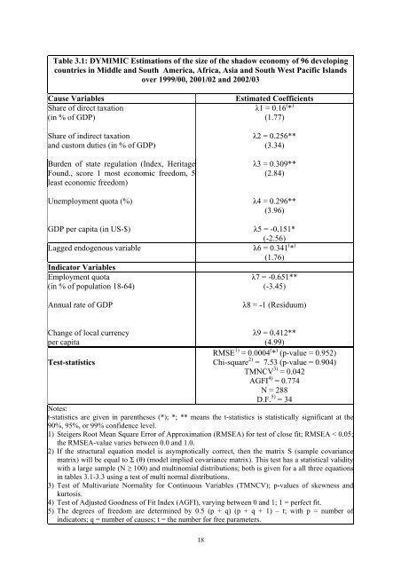
Table 3.1: DYMIMIC Estimations <strong>of</strong> <strong>the</strong> size <strong>of</strong> <strong>the</strong> shadow economy <strong>of</strong> 96 developing<br />
countries in Middle <strong>and</strong> South America, Africa, Asia <strong>and</strong> South West Pacific Isl<strong>and</strong>s<br />
over 1999/00, 2001/02 <strong>and</strong> 2002/03<br />
Cause Variables Estimated Coefficients<br />
Share <strong>of</strong> direct taxation λ1 = 0.16 ( * )<br />
(in % <strong>of</strong> GDP) (1.77)<br />
Share <strong>of</strong> indirect taxation λ2 = 0.256**<br />
<strong>and</strong> custom duties (in % <strong>of</strong> GDP) (3.34)<br />
Burden <strong>of</strong> state regulation (<strong>Index</strong>, Heritage<br />
Found., score 1 most economic freedom, 5<br />
least economic freedom)<br />
λ3 = 0.309**<br />
(2.84)<br />
Unemployment quota (%) λ4 = 0.296**<br />
(3.96)<br />
GDP per capita (in US-$) λ5 = -0.151*<br />
(-2.56)<br />
Lagged endogenous variable λ6 = 0.341 ( * )<br />
(1.76)<br />
Indicator Variables<br />
Employment quota λ7 = -0.651**<br />
(in % <strong>of</strong> population 18-64) (-3.45)<br />
Annual rate <strong>of</strong> GDP λ8 = -1 (Residuum)<br />
Change <strong>of</strong> local currency λ9 = 0.412**<br />
per capita (4.99)<br />
RMSE 1) = 0.0004 ( * ) (p-value = 0.952)<br />
Test-statistics Chi-square 2) = 7.53 (p-value = 0.904)<br />
TMNCV 3) = 0.042<br />
AGFI 4) = 0.774<br />
N = 288<br />
D.F. 5) = 34<br />
Notes:<br />
t-statistics are given in paren<strong>the</strong>ses (*); *; ** means <strong>the</strong> t-statistics is statistically significant at <strong>the</strong><br />
90%, 95%, or 99% confidence level.<br />
1) Steigers Root Mean Square Error <strong>of</strong> Approximation (RMSEA) for test <strong>of</strong> close fit; RMSEA < 0.05;<br />
<strong>the</strong> RMSEA-value varies between 0.0 <strong>and</strong> 1.0.<br />
2) If <strong>the</strong> structural equation model is asymptotically correct, <strong>the</strong>n <strong>the</strong> matrix S (sample covariance<br />
matrix) will be equal to Σ (θ) (model implied covariance matrix). This test has a statistical validity<br />
with a large sample (N ≥ 100) <strong>and</strong> multinomial distributions; both is given for a all three equations<br />
in tables 3.1-3.3 using a test <strong>of</strong> multi normal distributions.<br />
3) Test <strong>of</strong> Multivariate Normality for Continuous Variables (TMNCV); p-values <strong>of</strong> skewness <strong>and</strong><br />
kurtosis.<br />
4) Test <strong>of</strong> Adjusted Goodness <strong>of</strong> Fit <strong>Index</strong> (AGFI), varying between 0 <strong>and</strong> 1; 1 = perfect fit.<br />
5) The degrees <strong>of</strong> freedom are determined by 0.5 (p + q) (p + q + 1) – t; with p = number <strong>of</strong><br />
indicators; q = number <strong>of</strong> causes; t = <strong>the</strong> number for free parameters.<br />
18