5kk80 Assignment 2 – Design-Space Exploration

5kk80 Assignment 2 – Design-Space Exploration
1 Introduction
Eindhoven University of Technology
Department of Electrical Engineering
3 April 2008
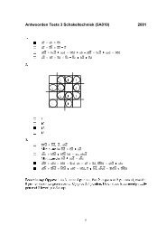
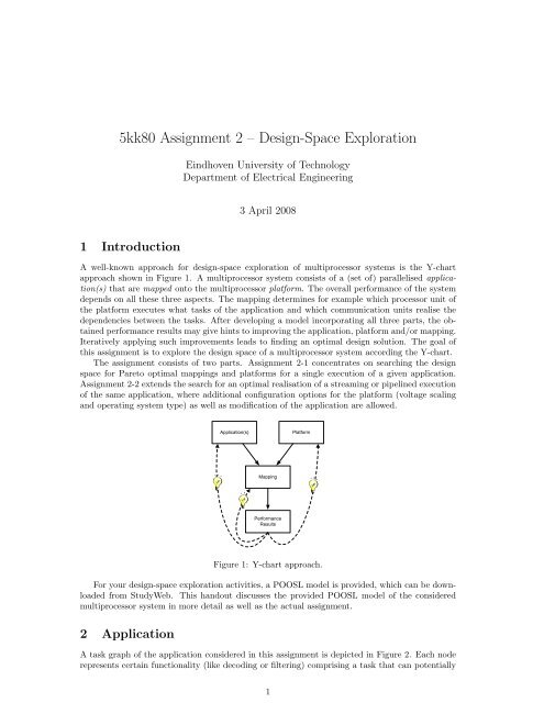
A well-known approach for design-space exploration of multiprocessor systems is the Y-chart
approach shown in Figure 1. A multiprocessor system consists of a (set of) parallelised application(s)
that are mapped onto the multiprocessor platform. The overall performance of the system
depends on all these three aspects. The mapping determines for example which processor unit of
the platform executes what tasks of the application and which communication units realise the
dependencies between the tasks. After developing a model incorporating all three parts, the obtained
performance results may give hints to improving the application, platform and/or mapping.
Iteratively applying such improvements leads to finding an optimal design solution. The goal of
this assignment is to explore the design space of a multiprocessor system according the Y-chart.
The assignment consists of two parts. Assignment 2-1 concentrates on searching the design
space for Pareto optimal mappings and platforms for a single execution of a given application.
Assignment 2-2 extends the search for an optimal realisation of a streaming or pipelined execution
of the same application, where additional configuration options for the platform (voltage scaling
and operating system type) as well as modification of the application are allowed.
Figure 1: Y-chart approach.
For your design-space exploration activities, a POOSL model is provided, which can be downloaded
from StudyWeb. This handout discusses the provided POOSL model of the considered
multiprocessor system in more detail as well as the actual assignment.
2 Application
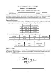
A task graph of the application considered in this assignment is depicted in Figure 2. Each node
represents certain functionality (like decoding or filtering) comprising a task that can potentially
1

e executed in parallel with other tasks. The edges represent dependencies between the tasks;
solid lines denote data dependencies, whereas dotted lines indicate control dependencies. Such
dependencies emerge from the communication of information between the tasks, which is implemented
using FIFO buffers. The unit of information that is exchanged between tasks is referred
to as a token, where each token contains 1 Byte of information. The dot with label 4 for buffer
F17 indicates that F17 already contains 4 tokens when the application is started. They allow a
streaming or pipelined execution of the application, where Task1 can be executed at maximum 4
times before Task7 must be executed.
Figure 2: Task graph with data and control dependencies.
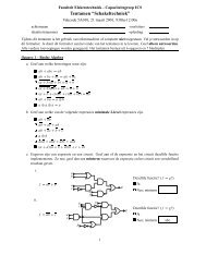
Figure 3: Markov chain for determining
scenarios in Task1.
The application in Figure 2 can operate in two modes or scenarios named S1 and S2. The
firing (execution) of a task starts with determining the scenario in which it will operate. Task1
determines the scenario based on the Markov chain (state machine with probabilities) in Figure 3.
This Markov chain models the real functionality of Task1 that interprets certain input data (which
may for example be read from a file) to determine the scenario. Each time Task1 fires, a transition
in the Markov chain is made, where the resulting state determines the scenario. All other tasks
determine the scenario by means of receiving a token from Task1 through their Control port (i.e.,
through the control dependencies in Figure 2). After fixing the scenario, a task continues with
receiving a token on all its other inputs. When all input data has become available, the actual
execution of the task can be performed by the processor node on which the task is mapped. After
completing the execution, the task finalises its firing with producing a token on all its outputs.
For Task1, this also includes sending tokens to the Control port of all other tasks valued with
the scenario in which they operate.
Not all tasks and dependencies are active in both scenarios. Task4 does not perform any
functionality in scenario S2 implying that also no information is communicated through buffers F5
and F12. Moreover, no information is exchanged through F9 in scenario S2. On the other hand,
F11 is inactive in scenario S1. In addition to these variations, the number of tokens produced
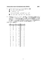
and consumed by the tasks using F8 differs for scenarios S1 and S2. A detailed overview of the
resource requirements for the tasks and buffers is given in Tables 1 and 2 respectively. Note that
the execution times in Table 1 are in cycles and not in seconds, see also Section 3.
In Assignment 2-1, only a single firing in scenario S1 of each task is considered (the Markov
chain in Figure 3 is not used). In Assignment 2-2, the application is to be executed continuously
in a streaming (pipelined) fashion, where all tasks concurrently fire in subsequent scenarios.
Task Graph Transformations Assignment 2-1 assumes that the task graph is fixed. For
many applications, it is however possible to adapt the task graph by exploiting for instance task
parallelism. Conversely, some of the overhead (like communication and task switching overhead)
incurred by the parallelisation can be reduced or eliminated by combining tasks. In Assignment
2

MIPS Scenario S1 Scenario S2
Task Exec. Time (Cycles) Mem. (Bytes) Exec. Time (Cycles) Mem. (Bytes)
Task1 60000 43008 52000 24576
Task2 18000 18432 46000 16384
Task3 24000 36864 55000 49152
Task4 40000 65536 0 0
Task5 85000 20480 65000 28672
Task6 70000 32768 120000 40960
Task7 90000 49152 85000 34816
ARM7 Scenario S1 Scenario S2
Task Exec. Time (Cycles) Mem. (Bytes) Exec. Time (Cycles) Mem. (Bytes)
Task1 40000 32768 48000 34816
Task2 18000 28672 32000 18432
Task3 15500 55296 28000 30720
Task4 24000 24576 0 0
Task5 32500 16384 55000 22528
Task6 64000 20480 46000 36864
Task7 56000 32768 48000 47104
TriMedia Scenario S1 Scenario S2
Task Exec. Time (Cycles) Mem. (Bytes) Exec. Time (Cycles) Mem. (Bytes)
Task1 72000 49152 48000 20480
Task2 15000 24576 32000 12288
Task3 20000 65536 40000 57344
Task4 64000 98304 0 0
Task5 96000 32768 56000 30720
Task6 108000 16384 64000 46080
Task7 80000 12288 98000 22528
Table 1: Resource requirements of the tasks.
2-2, the task graph in Figure 2 is assumed to be the most parallel version of the application.
From this most parallel version, it is allowed to adapt the task graph such that at maximum one
combination of two of the tasks Task2, Task3, Task4, Task5 and Task6 is performed.
Combining tasks affects the control and data dependencies as follows. Since all tasks receive the
same control token indicating the scenario in which they will operate, a single control dependency
is needed from Task1 (instead of two). On the other hand, all data dependencies with other tasks
remain valid, even if this implies multiple data dependencies between two tasks. For example, when
combining Task3 and Task4, one of the control dependencies through F4 and F6 can be removed,
whereas both data dependencies through F3 and F5 must remain to be modelled separately. Instead
of providing a list of profiling information for all allowed task combinations, the following approach
is used to derive the profiling information for the combined task as a rough approximation. On
any processor type and in each scenario, the execution time of the combined task equals the sum of
the execution times of the two original tasks, minus 10% (representing the reduction in overhead).
Similarly, the memory requirement for the combined task equals the maximum of the amount
of memory required by the original tasks, plus the number of tokens communicated between the
original tasks (if any). This approach is illustrated in Figure 4 when combining Task3 and Task4
into TaskX.
3 Platform
The platform considered in this assignment concerns a Network-on-Chip (NoC) based Multi-
Processor System-on-Chip (MPSoC) in a battery-powered embedded device. Four kinds of re-
3

Scenario S1 Scenario S2
Buffer # Tokens # Tokens
F1 2048 2048
F2 1 1
F3 1024 1024
F4 1 1
F5 2048 0
F6 1 1
F7 1 1
F8 1024 2048
Scenario S1 Scenario S2
Buffer # Tokens # Tokens
F9 4096 0
F10 2048 2048
F11 0 4096
F12 4096 0
F13 1 1
F14 3072 3072
F15 1024 1024
F16 1 1
F17 1 1
Table 2: Resource requirements of the buffers (Each token is 1 byte).
MIPS Scenario S1 Scenario S2
Task Exec. Time (Cycles) Mem. (Bytes) Exec. Time (Cycles) Mem. (Bytes)
TaskX 57600 65536 49500 49152
Figure 4: Transformed task graph with derived profiling information for a MIPS.
sources can be distinguished: processor units, communication units, storage units and an energy
source. The considered platform includes one energy resource (the battery), up to four processor
nodes and a NoC. The NoC of the considered platform provides point-to-point connections with
a guaranteed bandwidth and latency. Each node includes a processor unit that runs an operating
system on which tasks can be mapped. The processor unit has a private storage unit (data
memory) to store the code and context of the tasks. Moreover, a node includes a communication
unit on which buffers can be mapped that realise dependencies between the tasks that are mapped
on the processor unit. This communication unit has a private storage unit (buffer memory) to
store the information in the buffers mapped onto the node. On the other hand, the NoC only
includes a communication unit and a storage unit for mapping dependencies between tasks that
are mapped onto different nodes. Any processor, communication and storage unit drains energy
from the battery when it is used.
The platform has several parameters that can be set to obtain an optimal realisation of the
multiprocessor system. Next to the number of processor nodes that can be used, there is a choice
of three different processor types: MIPS, ARM7 and TriMedia 1 . Each processor type has different
characteristics, which are summarised in Table 3. The frequency in Table 3 denotes the base
frequency of the processor unit, while the context switching time refers to the number of cycles
it takes to initialise the execution of another task. The power consumption refers to the power
1 The processor specifications used in this assignment are fictitious. The names do not refer to real processors.
4

MIPS
Frequency 167000000 Cyles per Second
Context Switching Time 1500 Cycles
Power Consumption 0.075 Watt
ARM7
Frequency 100000000 Cyles per Second
Context Switching Time 1200 Cycles
Power Consumption 0.07 Watt
TriMedia
Frequency 200000000 Cyles per Second
Context Switching Time 3200 Cycles
Power Consumption 0.085 Watt
Table 3: Processor specifications.
that is used when the processor is switching tasks or executing a task. Another parameter for
each node is the type of scheduler in the operating system that runs on the processor. The
alternatives are FCFS (representing a first-come first serve scheduling policy without preemption)
and PB (denoting a priority-based scheduling policy with preemption). For the latter type of
scheduler, each task of the application must have a priority assigned to it, ranging from 1 to 7
(higher number means higher priority). The final parameter of a node is the voltage scaling factor
(sV ), which scales the base frequency and power consumption of the processor. Valid voltage
scaling factors for any processor type are 1/4, 1/3, 1/2, 2/3, 3/4 and 1/1. Although the platform
has some other parameters (like bandwidth per connection realised by a communication unit or the
power consumption per communicated and stored Byte), they should remain unchanged during the
assignment. Assignment 2-1 only allows changing the number of nodes and the type of processors,
while Assignment 2-2 also allows altering the operating system type (including priorities) and
voltage scaling factor.
Operating System The two types of schedulers that can be used for operating system running
on a processor are discussed in a bit more detail. A FCFS scheduler uses a FIFO queue to store ready
tasks, which denote the execution requests that are obtained from the different tasks that are ready
to execute. These requests are put into the queue in the order of reception. In case a request
is available in the queue, the first execution request is granted by executing the corresponding
task without interruptions. An advantage of this type of scheduler is that it is relatively easy to
implement. A disadvantage is that a higher priority task from which an execution request was
received later than a low priority task has to wait until execution of the lower priority task is
finished. The PB scheduler overcomes the latter disadvantage by allowing preemption of any lower
priority task. Instead of a FIFO queue, a PB scheduler maintains a list of execution requests that
is ordered 2 according to the priorities of the involved tasks. Though being more influenceable by
a programmer, a PB scheduler is slightly more difficult to implement. Moreover, preempting a
running task comes at the price of additional context switching, while the memory used by a task
is only freed after completing its execution. Many other schedulers exist for operating systems,
often being much more complex. In the first part of the assignment, only PB schedulers are used,
where the priority of Taski is set equal to i.
Voltage Scaling Changing the supply voltage of the processor units allows trading the energy
used for a given computation load against the execution time. To explain voltage scaling in
more detail, consider that the clock frequency f at which an integrated circuit can operate is
roughly proportional to the supply voltage V for some constant Kf , that is f = Kf · V . Recall
that the energy stored in a capacitor C equals 1
2 · C · V 2 (i.e., proportional to the square of the
2 The PB scheduler orders multiple tasks with equal priority in a (non-preemptive) FIFO fashion.
5

voltage over the capacitor). Therefore, the power P consumed by a processor as the result of
charging and discharging connections is proportional to the square of its supply voltage as well
as to the frequency at which this takes place: P = KP · V 2 · f for some constant KP . As a
result, it can be advantageous to reduce the supply voltage to a processor if the processor has idle
time; frequency (execution speed) can be exchanged for smaller power consumption. Suppose a
processor needs to perform a certain workload of W cycles as indicated in Table 1. The time t
to perform this workload is t = W/f = W/(Kf · V ). The energy E used during that time equals
E = P · t = KP · V 2 · f · W/f = KP · V 2 · W . Now, assume that VB denotes the base supply voltage
and sV the voltage scaling factor, that is V = sV · VB. Then, E = KP · (sV · VB) 2 · W = s2 V · EB,
where EB = KP · V 2 B · W being the base energy used for workload W . The time it takes to execute
the task is t = W/(Kf · V ) = W/(Kf · sV · VB) = tB/sV , where tB = W/(Kf · VB) is the execution
time for the base frequency and supply voltage. Thus, scaling the voltage by a factor sV increases
the execution time by a factor 1/sV and saves energy by a factor of s2 V . From an energy point of
view, a parallel implementation on multiple, slower processors is therefore preferred over a single
very fast processor. This is one of the primary motivations for using MPSoCs. Note also that a
solution that is too fast can be improved by decreasing the voltage scaling factor to make it slower,
while also reducing power consumption. Similarly, a solution that is too slow can be made faster
by increasing the voltage scale factor at the expense of additional power consumption.
4 Mapping
Given a particular (set of) application(s) and platform, the mapping describes which processor
unit, communication unit and storage unit is/are used to realise the execution of tasks and the
communication of tokens. For the considered multiprocessor system, it is only necessary to specify
which tasks of the application are mapped onto which processor nodes since the mapping of
buffers as well as which storage units are used to store what information can be derived from
that automatically. As discussed in Section 3, processor units and communication units have
private memories to store the tasks and tokens respectively. Moreover, each node includes a
communication unit that realises all dependencies between tasks that are mapped on that node,
while all dependencies between tasks mapped on different nodes must be realised by the NoC.
5 Performance Metrics
Application Next to the task graph, an application is characterised by a number of performance
constraints. The following constraints are to be satisfied:
• Latency: ≤ 1/500 seconds;
• Throughput: ≥ 800 Firings of Task7 per second;
• Deadline Miss Probability: ≤ 5%.
Latency is defined here as the time between starting the first firing of Task1 and the corresponding
completion of Task7. In general, the latency can be larger than the time between two
executions of Task1 in case of streaming (pipelined) execution. The throughput indicates the
average number of firings of Task7 per second in such case. Since the application can operate
in different scenarios, there is some variation in the latency possible. Hence, the deadline for the
next completion of Task7 may be missed, but on average, not more than 5% of those completions
are allowed to be late.
Platform Apart from the constraints for the application, there are some optimisation criteria for
the platform. The optimisation criteria for the platform are (in order of importance): (1) energy or
power consumption and (2) amount of resources. The latter refers, amongst others, to the number
of processor units, the size of storage units and the number of concurrent connections to be served
6

y communication units. The overall goal therefore is to look for the minimal configuration of
the system that satisfies the constraints, thereby consuming as little power as possible. Hence, it
makes sense to define some performance metrics for the platform to identify bottlenecks:
• Processor Unit: average utilisation;
• Storage Unit: maximum and average occupancy;
• Communication Unit: maximum and average number of concurrently served connections;
• Battery: peak and average power consumption, where the latter equals the amount of
energy consumed in 1 second.
6 Assignment
This assignment consists of two parts. The provided POOSL model, which is discussed in more
detail in Section 7, forms the starting point for both parts.
Part 1 Assignment 2-1 aims at exploring the trade-off between energy consumption, latency
and number of processor nodes for alternative mappings and processor nodes of different types,
considering a single execution of each task of the application in scenario S1. Use the provided
POOSL model to explore the space of potential solutions that satisfy the latency and deadline
miss constraints for the application and determine a set of feasible, Pareto-optimal configurations
(platform description + mapping).
Recall that in this part of the assignment, the processor units may only use the PB scheduler
type of operating system (where the priority of Taski equals i) and the voltage scaling factors
equal 1/1. Transformation of the task graph is also not considered in this part.
Part 2 In Assignment 2-2, the design space is extended with the possibility to transform the
task graph, alternative operating systems (including priorities) and voltage scaling options (which
can be set individually for each of the different nodes). The goal is to find a single optimal solution
in terms of power consumption and amount of resources, subject to the throughput and deadline
miss constraints for the application, which is now executed in a streaming fashion.
Ultimately, 2 June at 9.00h AM, you need to have delivered a short report on your findings
(max. 8 pages, excluding graphs) together with at least the POOSL models that represent your
optimal design solution(s) for both assignment parts, by means of submission to StudyWeb. Please
submit your work as a single zip archive via the Assignment2/Submit folder. Studyweb
confirms the correct submission of your work. It is then timestamped and moved to a folder not
visible to you. Please do not resubmit if Studyweb confirmsthe sucessful submission of you file.
Taking the guidelines for documenting experimental research into account, the (individually)
written report should elaborate on at least following aspects for both parts of the assignment:
• The tradeoffs that you have discovered and the resulting design solution(s)
• The approach you used to search the design space for finding your design solution(s), including
an argumentation why you selected this approach
• The impact of streaming execution, task graph transformations, different operating system
types and voltage scaling (Discuss your hypotheses about these aspects in relation to results
you obtained for Assignment 2-1)
• The adequacy of abstractions made in the provided model regarding the platform. So,
how well does the model represent a real battery-powered NoC-based MPSoC? One may
for example investigate what abstractions are made in the NoC model for Assignment 2 in
7

comparison to those used in Assignment 1 and what impact these abstractions may have on
the obtained performance results
If you still have questions, you may contact Bart Theelen (B.D.Theelen@tue.nl) or Marc
Geilen (M.C.W.Geilen@tue.nl). You may also exploit the office hours every Wednesday between
12:30h and 13:30h in PT 9.19. Please announce your visit via B.D.Theelen@tue.nl.
7 Provided Model
This section discusses the provided POOSL model and how it can be used to complete the assignment.
The screen shot of SHESim in Figure 5 shows that it includes a representation of
the Application and the NoC-based MPSoC platform. The SimulationController process is
concerned with terminating the simulation whenever the estimation results for all average performance
metrics have become accurate and is not really a part of the system. It also terminates the
simulation if not all estimations have become accurate after simulating 50 units of model time.
7.1 Application Model
Figure 5: Top-level diagram for the provided model.
The Application cluster models the task graph of Figure 2 and has the following instantiation
parameters that are relevant for performing the assignment:
• Iterate - controls whether to execute the task graph in a streaming fashion or not. Iterate
should be set to false for Assignment 2-1 and to true in Assignment 2-2;
• MapTaskiTo - indicates on which processor node task i is mapped and hence, the possible
values are "Node1", "Node2", "Node3" and "Node4" (Note that these are Strings; don’t
forget to include the double quotes);
• PriorityTaski - is the integer priority of task i, where a higher number refers to a higher
priority.
The Application cluster captures the structure of processes modelling the tasks and buffers
of Figure 2. The process Task7 includes a monitor to evaluate the percentage of deadline misses
and the throughput metric defined in Section 5. In addition, the latency metric is evaluated in
8

case the Iterate instantiation parameters equals false. The monitoring results can be observed
by inspecting the instance variable Status. On the other hand, the estimation results are logged
to a file named Application.log. Note that no throughput estimation can be given for a single
iteration of the application (i.e., for Assignment 2-1).
Modelling Combined Tasks When performing task graph transformations, it is necessary to
adapt process class Task1 and define a new process class for the combined task before instantiating
it in the Application cluster. To enable doing so, the modelled protocols for communicating with
buffers and processor nodes must be obeyed. Note that you must have opened the cluster
class browser on Application when modifying class Task1 because of a bug in SHESim.
Modifying Task1 is relatively easy and only involves changes to the NotifyBuffersAbout-
Mapping, ReserveSpaceForWrites and PerformWrites methods to ensure that communication
through the control dependency in Figure 2 that has become obsolete is not performed anymore.
For any task, the method NotifyBuffersAboutMapping enables automatic determination
of the mapping of the buffers connected to it. Hence, for Task1, it is necessary to remove the
concurrent activity on sending of the MappedTo message to the involved obsolete buffer. In the
ReserveSpaceForWrites, the concurrent activity on sending the ReserveRoom message and consecutively
receiving the ReservationSuccessful message must be removed. Finally, in method
PerformWrites, the statement for sending the WriteToken message must be removed.
Defining a process class (let’s assume that it is called TaskX) to model the new combined
task can best be based on defining a subclass of Task (and using an existing Task class definition
as a reference). This process class provides a template that is used for defining all other
tasks (except for Task1) in the provided model. When doing so, defining class TaskX only involves
overloading methods NotifyBuffersAboutMapping, CheckTokenAvailabilityForReads,
ReserveSpaceForWrites, ReleaseSpaceForReads and PerformWrites while the reception of
the token from the Control port and the communication with the processor node is already
defined in the superclass Task. Method NotifyBuffersAboutMapping must include a concurrent
activity for informing each buffer connected to TaskX about its mapping. This concurrent
activity concerns the sending of a message MappedTo with MapTo as parameter. The method
CheckTokenAvailabilityForReads models the request and acknowledgement with the buffer at
each input of TaskX about the availability of a token. The protocol prescribes to send the request as
a message InspectTokenAvailability and then receive the acknowledgement by means of a message
TokenAvailable with some parameter of class Token. The method ReserveSpaceForWrites
involves the specification of a concurrent activity for informing the buffer at each output of TaskX
about the intention to write a token after completing execution. Such a concurrent activity models
the request and acknowledgement regarding the reservation of buffer space. The protocol
prescribes to send the request by means of a message ReserveSpace with a parameter that represents
the token to be written (or more precisely, the size of the token to be written). To this
end, a new object of class Token must be created and its size in Bytes (see also Table 2) must be
initialised using data method setSize. The acknowledgement is modelled by receiving message
ReservationSuccessful. The method ReleaseSpaceForReads models informing the buffer at
all inputs about the completion of the execution of the task and hence that the space for the
read token can be released by sending a message ReleaseSpace to all inputs. Finally, method
PerformWrites informs the buffer at all outputs about the fact that the produced tokens have
become available for consumption by the target tasks.
After defining process class TaskX, an instance can be created in the Application. What remains
to be done is properly connecting the new process with the involved buffers and initialising its
instantiation parameters. Instantiation parameter Name should be a String indicating the task’s
name, that must match with the new entry in the processor specification files MIPS.txt, ARM7.txt
and TriMedia.txt, see also Section 7.2. The instantiation parameters MapTo and Priority initialise
the processor node to which the new task is mapped and the priority of the task respectively.
9

7.2 Platform Model
Figure 6: Cluster class Platform.
The MPSoC cluster in Figure 5 models the considered battery-powered NoC-based MPSoC platform
with at maximum four processor nodes. Figure 6 gives a screen dump of the Platform cluster
class definition indicating the models of the battery, NoC and four processor nodes. Note that
although four processor nodes (i.e., Node1, Node2, Node3 and Node4) are instantiated in the
Platform model, the mapping determines how many nodes are actually used 3 . The process
PlatformMonitor is concerned with terminating the simulation whenever the estimation results
for all average performance metrics have become accurate and is not really a part of the system.
The ProcessorNode cluster class has the following relevant instantiation parameters:
• ProcessorType - denotes the type of processor unit in the node. The possible values are
"MIPS", "ARM7" and "TriMedia" (Note that these are Strings);
• OSPolicy - indicates the type of scheduler for the operating system running on the processor
unit. The possible values are "PB" and "FCFS" (Note that these are Strings);
• VoltageScaleFactor - concerns the voltage scaling factor. Possible values are 1/4, 1/3,
1/2, 2/3, 3/4 and 1/1 (Note that these must be Reals and hence, use e.g. 1/1 or 1.0).
The Battery includes a monitor to evaluate the performance metrics defined in Section 5
by means of the Status instance variable. The estimation results for these performance metrics
are also logged in the file Battery.log. Note that a single iteration of the application will not
provide sufficient information to properly estimate the average power consumption with a detailed
accuracy indication. In this case, only the average power consumption that was observed during
the particular simulation run is provided without any accuracy details. The other resources of
the platform also include monitors, though whether they produce results depends on whether
something is mapped onto the involved resource. The processor utilisation and data memory
occupancy results are logged in files named ProcessorNodei.log, where i is the number of the
node. On the other hand, the utilisation of the communication unit and buffer memory occupancy
results are logged in files named CommunicationNodei.log, where i is again the number of the
3 The instantiated processor, memory and communication resources of an unused node will not consume power.
10

node. Finally, the utilisation of the communication unit and buffer memory occupancy results for
the NoC are logged in file named CommunicationNoC.log.
Processor Specifications The specification of the processor types and corresponding profiling
information for the different tasks in Tables 3 and 1 are stored in the files MIPS.txt, ARM7.txt
and TriMedia.txt. When simulating with SHESim, these 3 processor specification files must be
located in the directory where the image file (originally named SHESim.im) is located. When using
the Rotalumis tool, the 3 processor specification files must be located in the directory where the
exported model file with extension .p4r (default name is model.p4r) is located.
Specifying Combined Tasks When performing task graph transformations, it is necessary to
add the profiling information derived for the combined task as illustrated in Figure 4 to the files
MIPS.txt, ARM7.txt and TriMedia.txt in a similar way as for the original tasks. Ensure that
you use the same task name (between double quotes) in the first column as you used to initialise
the instantiation parameter of the process modelling the new task in the Application.
11