Making regression tables simplified
Making regression tables simplified
Making regression tables simplified

You also want an ePaper? Increase the reach of your titles
YUMPU automatically turns print PDFs into web optimized ePapers that Google loves.
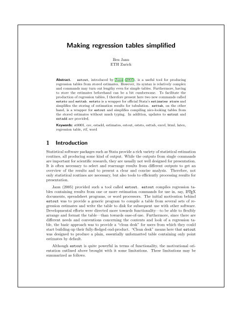
<strong>Making</strong> <strong>regression</strong> <strong>tables</strong> <strong>simplified</strong><br />
Ben Jann<br />
ETH Zurich<br />
Abstract. estout, introduced by Jann (2005), is a useful tool for producing<br />
<strong>regression</strong> <strong>tables</strong> from stored estimates. However, its syntax is relatively complex<br />
and commands may turn out lengthy even for simple <strong>tables</strong>. Furthermore, having<br />
to store the estimates beforehand can be a bit cumbersome. To facilitate the<br />
production of <strong>regression</strong> <strong>tables</strong>, I therefore present here two new commands called<br />
eststo and esttab. eststo is a wrapper for official Stata’s estimates store and<br />
simplifies the storing of estimation results for tabulation. esttab, on the other<br />
hand, is a wrapper for estout and simplifies compiling nice-looking <strong>tables</strong> from<br />
the stored estimates without much typing. In addition, updates to estout and<br />
estadd are provided.<br />
Keywords: st0001, csv, estadd, estimates, estout, eststo, esttab, excel, html, latex,<br />
<strong>regression</strong> table, rtf, word<br />
1 Introduction<br />
Statistical software packages such as Stata provide a rich variety of statistical estimation<br />
routines, all producing some kind of output. While the outputs from single commands<br />
are important for scientific research, they are usually not well designed for presentation.<br />
It is often necessary to select and rearrange results from different outputs to get an<br />
overview of the results and to present a clear and concise analysis. Therefore, not<br />
only statistical routines are necessary, but also tools to efficiently processing results for<br />
presentation.<br />
Jann (2005) provided such a tool called estout. estout compiles <strong>regression</strong> <strong>tables</strong><br />
containing results from one or more estimation commands for use in, say, L ATEX<br />
documents, spreadsheet programs, or word processors. The initial motivation behind<br />
estout was to provide a generic program to compile a table from several sets of <strong>regression</strong><br />
estimates and write the table to disk for subsequent use with other software.<br />
Developmental efforts were directed more towards functionality—to be able to flexibly<br />
arrange and format the table—than towards ease-of-use. Furthermore, since there are<br />
different needs and conventions concerning the contents and look of a <strong>regression</strong> table,<br />
the basic approach was to provide a “clean desk” for users from which they could<br />
start building-up their fully-fledged end-product. “Clean desk” means here that estout<br />
was designed to produce a plain, essentially unformatted table containing only point<br />
estimates by default.<br />
Although estout is quite powerful in terms of functionality, the motivational orientation<br />
outlined above brought with it some limitations. These limitations may be<br />
summarized as follows.
2 <strong>Making</strong> <strong>regression</strong> <strong>tables</strong> <strong>simplified</strong><br />
1. estout <strong>tables</strong> are usually not suitable for display in Stata’s results window. For<br />
example, by default, estout uses the tab-character to separate the table’s columns.<br />
However, tab-characters are expanded to a fixed amount of blanks in the results<br />
window, causing the table’s columns to appear misaligned. This is unfavorable<br />
because it is often purposeful to produce <strong>regression</strong> <strong>tables</strong> on the fly, for quick<br />
results inspection on screen.<br />
2. estout’s syntax is not as intuitive and user-friendly as it could be. For example,<br />
there are nested options, which do their job, but are hard to handle and hard to<br />
remember. Also even experienced users are often forced to consult the command’s<br />
documentation while producing an estout table.<br />
3. The amount of typing required to compile even a simple table can be quite considerable.<br />
Users generally have to specify many options to determine the content<br />
and formatting of the table according to their needs. Note that estout provides<br />
the possibility to pre-specify options via so-called defaults files (similar to scheme<br />
files for Stata graphics). However, maintaining such defaults files does not appear<br />
beneficial unless one is working on large reports containing lots of similar <strong>tables</strong>.<br />
A consequence of these limitations is that the use of estout may be somewhat<br />
clumsy in daily work. In addition, smooth application of estout is compromised by the<br />
fact that the estimation sets have to be stored using official Stata’s estimates store<br />
before they can be tabulated (at least if there is more than one set of estimates). A<br />
drawback of estimates store is that it requires the user to specify names under which<br />
to store the estimation sets. Having to provide such names, although sensible in some<br />
contexts, can be distracting.<br />
To summarize, there seems to be a need for (1) an easy-to-use version of estout<br />
that produces fully formatted <strong>tables</strong> right away and is suitable for interactive work, and<br />
(2) a <strong>simplified</strong> procedure to hold on to estimates for tabulation. In the remainder of<br />
this text I will address these two points (in reverse order) and present in Section 2 a<br />
command called eststo to overcome the limitations of estimates store. Section 3<br />
then introduces a user-friendly estout wrapper called esttab and illustrates its application<br />
by examples. The Appendix (Section 4) contains syntax overviews for the two<br />
commands and provides updates to estout and estadd.<br />
Space limitations do not allow an extended treatment of the new commands. For<br />
details and additional examples consult the online help or visit the estout web site at<br />
http://fmwww.bc.edu/repec/bocode/e/estout/.<br />
2 eststo: Storing estimates <strong>simplified</strong><br />
The new eststo command stores a copy of the active estimation results for later tabulation.<br />
It is an alternative to official Stata’s estimates store. The basic syntax of<br />
eststo is
Jann 3<br />
eststo � name � � , options � � : estimation command �<br />
Store estimates without providing a name<br />
A main advantage of eststo over estimates store is that it does not require the user<br />
to specify a name for the stored estimates. If name is provided, then, naturally, the<br />
estimates are stored under this name. However, if no name is provided, eststo makes<br />
up its own name. Note that eststo keeps track of the names of the stored estimation<br />
sets via global macros from where the names can be picked up by, say, estout. Here is<br />
an example:<br />
. sysuse auto<br />
(1978 Automobile Data)<br />
. regress price weight mpg<br />
(output omitted )<br />
. eststo<br />
(est1 stored)<br />
. regress price weight mpg foreign<br />
(output omitted )<br />
. eststo<br />
(est2 stored)<br />
. estout, style(fixed)<br />
est1 est2<br />
b b<br />
weight 1.746559 3.464706<br />
mpg -49.51222 21.8536<br />
foreign 3673.06<br />
_cons 1946.069 -5853.696<br />
To erase the estimation sets that have been stored by eststo, type<br />
. eststo clear<br />
Use eststo as a prefix command<br />
As is illustrated in the example above, a model’s results are stored by applying eststo<br />
after the model has been fitted. This is also how official estimates store works.<br />
Alternatively, however, eststo may be used as a prefix command (see [U] 11.1.10<br />
Prefix commands). For example:<br />
. eststo: regress price weight mpg<br />
(output omitted )<br />
. eststo: regress price weight mpg foreign<br />
(output omitted )<br />
. estout, style(fixed)<br />
est1 est2<br />
b b<br />
weight 1.746559 3.464706<br />
mpg -49.51222 21.8536
4 <strong>Making</strong> <strong>regression</strong> <strong>tables</strong> <strong>simplified</strong><br />
foreign 3673.06<br />
_cons 1946.069 -5853.696<br />
Note that by (see [D] by) is allowed with eststo, if eststo is used as a prefix<br />
command. Furthermore, note that eststo has an option to drop the e(sample) from<br />
the stored estimation sets to preserve memory. 1<br />
3 esttab: Tabulating estimates <strong>simplified</strong><br />
The new esttab command is a wrapper for estout. Its syntax is much simpler than<br />
that of estout and, by default, it produces publication-style <strong>tables</strong> that display nicely<br />
in Stata’s results window. Note that esttab is more than just a <strong>simplified</strong> version of<br />
estout. On the one hand, esttab provides full estout functionality since all estout<br />
options are, in fact, allowed in esttab. On the other hand, esttab also extends functionality.<br />
For example, esttab adds support for Word RTF and Excel CSV and provides<br />
improved functionality for L ATEX and HTML.<br />
In what follows I will try to give a brief introduction to esttab and illustrate some<br />
of its applications, although I will only be able to scratch the surface. See the Appendix<br />
for a syntax overview and consult the online help for more detailed information. Further<br />
examples can also be found at http://fmwww.bc.edu/repec/bocode/e/estout/.<br />
Basic syntax and usage<br />
The syntax of esttab is<br />
esttab � namelist � � using filename � � , options estout options �<br />
where namelist is a list of names of stored estimation sets. namelist may be * to tabulate<br />
all stored estimation sets. If namelist is omitted, esttab tabulates the currently active<br />
estimates or, if present, the estimation sets stored by eststo. Specifying using causes<br />
the <strong>regression</strong> table to be written to a file on disk instead of being displayed in Stata’s<br />
results window.<br />
Analogous to estout (or official Stata’s estimates table), the basic procedure is<br />
to first store a number of models and then apply esttab to these stored estimation<br />
sets to compose a <strong>regression</strong> table. The great difference between esttab and estout,<br />
however, is that, if applied without any options, esttab produces a fully formatted<br />
table. Consider the following example and compare it to the examples in Section 2, in<br />
1. Stored estimates consume a considerable amount of memory. In order to preserve full functionality<br />
of postestimation commands (see [U] 20 Estimation and postestimation commands), an estimation<br />
sample indicator variable (i.e. a copy of the e(sample) function) is stored for each estimation<br />
set. Even though byte storage type is used for these variables, they may blow up the dataset if it<br />
contains a large number of observations or if many estimation sets are stored. Additionally, storing the<br />
e(sample) information has the side effect of slowing down cycling through the stored estimation sets in<br />
large datasets, which also slows down tabulation programs such as estout or official Stata’s estimates<br />
table.
Jann 5<br />
which estout was used:<br />
. sysuse auto<br />
(1978 Automobile Data)<br />
. eststo: regress price weight mpg<br />
(output omitted )<br />
. eststo: regress price weight mpg foreign<br />
(output omitted )<br />
. esttab<br />
(1) (2)<br />
price price<br />
weight 1.747** 3.465***<br />
(2.72) (5.49)<br />
mpg -49.51 21.85<br />
(-0.57) (0.29)<br />
foreign 3673.1***<br />
(5.37)<br />
_cons 1946.1 -5853.7<br />
(0.54) (-1.73)<br />
N 74 74<br />
t statistics in parentheses<br />
* p
6 <strong>Making</strong> <strong>regression</strong> <strong>tables</strong> <strong>simplified</strong><br />
Standard errors in parentheses<br />
The t statistics can also be replaced by p-values (p), confidence intervals (ci), or any<br />
parameter statistics contained in the estimates (see the aux() option). Further summary<br />
statistics options are, for example, pr2 for the pseudo R-squared and bic for<br />
Schwarz’s information criterion. Moreover, there is a generic scalars() option to<br />
include any other scalar statistics contained in the stored estimates. For instance,<br />
scalars(F df m df r) would add the overall F statistic and information on the degrees<br />
of freedom.<br />
Also the point estimates may be replaced by other statistics. Here is an example in<br />
which beta coefficients are printed and the t statistics are suppressed:<br />
. esttab, beta not<br />
(1) (2)<br />
price price<br />
weight 0.460** 0.913***<br />
mpg -0.097 0.043<br />
foreign 0.573***<br />
N 74 74<br />
Standardized beta coefficients<br />
* p
Jann 7<br />
to fit more models on screen without line breaking. Other options are, for example,<br />
label to cause variable labels to be used and mtitles() to specify model titles to be<br />
printed in the header above the model columns. Example:<br />
. esttab, se ar2 nostar brackets label title(This is a <strong>regression</strong> table)<br />
> nonumbers mtitles("Model A" "Model B") addnote("Source: auto.dta")<br />
This is a <strong>regression</strong> table<br />
Model A Model B<br />
Weight (lbs.) 1.747 3.465<br />
[0.641] [0.631]<br />
Mileage (mpg) -49.51 21.85<br />
[86.16] [74.22]<br />
Car type 3673.1<br />
[684.0]<br />
Constant 1946.1 -5853.7<br />
[3597.0] [3377.0]<br />
Observations 74 74<br />
Adjusted R-squared 0.273 0.478<br />
Standard errors in brackets<br />
Source: auto.dta<br />
Numerical formats<br />
esttab has sensible default settings for numerical display formats. For example, t statistics<br />
are printed using two decimal places and R-squared measures are printed using three<br />
decimal places. For point estimates and, for example, standard errors an adaptive display<br />
format is used where the number of displayed decimal places depends on the scale<br />
of the statistic to be printed (the default format is a3; see below).<br />
The format applied to a certain statistic can be changed by adding the appropriate<br />
display format specification in parentheses. For example, to display p-values and the<br />
R-squared using four decimal places and display point estimates using the %9.0g format,<br />
type<br />
. esttab, b(%9.0g) p(4) r2(4) nostar wide<br />
(1) (2)<br />
price price<br />
weight 1.746559 (0.0081) 3.464706 (0.0000)<br />
mpg -49.51222 (0.5673) 21.8536 (0.7693)<br />
foreign 3673.06 (0.0000)<br />
_cons 1946.069 (0.5902) -5853.696 (0.0874)<br />
N 74 74<br />
R-sq 0.2934 0.4996<br />
p-values in parentheses
8 <strong>Making</strong> <strong>regression</strong> <strong>tables</strong> <strong>simplified</strong><br />
Available formats are official Stata’s display formats, such as %9.0g or %8.2f (see<br />
[D] format). Alternatively, as is illustrated in the example above, a fixed format can<br />
be requested by specifying a single integer indicating the desired number of decimal<br />
places. Furthermore, an adaptive format, a#, may be specified, where # in {1, . . . , 9}<br />
determines the minimum number of “significant digits” to be printed.<br />
Document formats<br />
Output format options in esttab allow the user to quickly switch between different<br />
document formats depending on the table’s intended use. Available formats are:<br />
smcl to produce an SMCL formatted table. smcl is the default (unless using is specified)<br />
and is used to display the table in Stata’s results window.<br />
fixed to produce a fixed-format ASCII table. This is suitable, for example, if the table<br />
is to be displayed in a fixed-font text editor.<br />
tab to produce a tab-delimited ASCII table. This is a general format that can be used<br />
as an input format for many programs.<br />
csv to produce a CSV (Comma Separated Value format) table for use with Excel.<br />
Delimiter is a comma. See below for details on using esttab with Excel.<br />
scsv to produce a CSV table using a semicolon as the delimiter. This is appropriate<br />
for some non-English versions of Excel such as the German version.<br />
rtf to produce a Rich Text Format table for use with word processors. The code follows<br />
the guidelines in Burke (2003) and should work with about any RTF viewer. See<br />
below for details on using esttab with Word.<br />
html to produce a simple HTML-formatted table that can be displayed in a web browser.<br />
tex to produce a table to be included in a L ATEX 2ε document. See below for details on<br />
using esttab with L ATEX.<br />
booktabs to produce a L ATEX 2ε-formatted table for use with L ATEX’s booktabs package. 2<br />
A specific document format can be chosen by specifying the format’s name as an<br />
option to esttab. For example,<br />
. esttab, tab<br />
(output omitted )<br />
produces a tab-delimited table. As indicated above, the smcl mode is the default.<br />
However, if using filename is specified, the default format depends on filename’s suffix<br />
(e.g. rtf for “.rtf”, html for “.htm” or “.html”). Furthermore, if filename is specified<br />
without suffix, a default suffix is added depending on the specified document format<br />
(e.g. “.tex” for tex or booktabs).<br />
2. See http://www.ctan.org/tex-archive/macros/latex/contrib/booktabs/.
Jann 9<br />
Use with Excel<br />
To produce a table for use with Excel, apply the csv format (or the scsv format<br />
depending on the language version of Excel). For example, type<br />
. esttab using example.csv<br />
(output written to example.csv)<br />
and then click on “example.csv” in Stata’s results window to launch Excel and display<br />
the file’s content.<br />
Note that, depending on whether the plain option is specified or not, esttab uses<br />
two different variants of the CSV format. By default, that is, if plain is omitted, the<br />
contents of the table cells are enclosed in double quotes preceded by an equal sign (i.e.<br />
="..."). This prevents Excel from trying to interpret the contents of the cells and,<br />
therefore, preserves formatting elements such as parentheses around t statistics. One<br />
drawback of this approach is, however, that the displayed numbers cannot directly be<br />
used for further calculations in Excel. Hence, if the purpose of exporting the estimates<br />
is to do additional computations in Excel, specify the plain option. In this case, the<br />
table cells are enclosed in double quotes without the equal sign, and Excel will interpret<br />
the contents as numbers.<br />
Use with Word<br />
To produce a table for use with Word, apply the rtf format. For example, type<br />
. esttab using example.rtf<br />
(output written to example.rtf)<br />
and then click on “example.rtf” in Stata’s results window to launch Word (or another<br />
RTF Reader, depending on your operating system settings) and display the table. Note<br />
that you may use estout’s varwidth(#) and modelwidth(#) options to change the<br />
column widths in the RTF table (# = 12 corresponds to a column width of one inch,<br />
save cell padding). Furthermore, you may use the append option to include several<br />
<strong>tables</strong> in one RTF document.<br />
Use with L ATEX<br />
Using esttab together with L ATEX can be very effective. For example, Table 1 in this<br />
document has been produced by running the command<br />
. esttab using example1.tex, label nostar title(Regression table\label{tab1})<br />
(output written to example1.tex)<br />
and including<br />
\input{example1.tex}<br />
in the L ATEX code.
10 <strong>Making</strong> <strong>regression</strong> <strong>tables</strong> <strong>simplified</strong><br />
Table 1: Regression table<br />
(1) (2)<br />
Price Price<br />
Weight (lbs.) 1.747 3.465<br />
(2.72) (5.49)<br />
Mileage (mpg) -49.51 21.85<br />
(-0.57) (0.29)<br />
Car type 3673.1<br />
(5.37)<br />
Constant 1946.1 -5853.7<br />
(0.54) (-1.73)<br />
Observations 74 74<br />
t statistics in parentheses<br />
Note that esttab automatically initializes the tabular environment and, if title()<br />
is specified, sets the table as a float object. Use the fragment option if you prefer to<br />
hard-code the table’s environment and have esttab just produce the table rows.<br />
Table 1 looks alright, but there is room for improvement. For example, the vertical<br />
spaces after the horizontal lines seem too small, the vertical gaps between the coefficients<br />
appear too large, and the use of double lines is debatable. One remedy for these problems<br />
is to load L ATEX’s booktabs package in the document preamble and choose the booktabs<br />
format in esttab.<br />
Other improvements to Table 1 would be to use a typographical minus sign and to<br />
align the numbers on the decimal point. These improvements can be implemented, for<br />
example, by loading L ATEX’s dcolumn package 3 and using esttab’s alignment() option<br />
to set a D column specifier. For instance, a good result might be attained by<br />
. esttab using example2.tex, booktabs alignment(D{.}{.}{-1})<br />
(output written to example2.tex)<br />
Last but not least, it can be desirable to space out the table columns to a certain<br />
total table width. This is achieved using esttab’s width() option. For example, type<br />
. esttab using example3.tex, width(0.6\hsize)<br />
(output written to example3.tex)<br />
to set the table width to 60% of the width of the text body and add white space between<br />
the columns.<br />
3. See http://www.ctan.org/tex-archive/macros/latex/required/tools/.
Jann 11<br />
Viewing the internal estout call<br />
Sometimes, a desired table cannot be produced with standard esttab options right<br />
away. One approach in such cases is to use esttab to assemble a table that comes close,<br />
and then hand-edit and re-run the estout call that has been compiled by esttab.<br />
The estout call can be made visible by the noisily option and is also returned in<br />
r(estout). Example:<br />
. esttab, noisily<br />
estout ,<br />
cells(b(fmt(a3) star) t(fmt(2) par("{ralign 12:{txt:(}" "{txt:)}}")))<br />
stats(N, fmt(%18.0g) labels(‘"N"’))<br />
starlevels(* 0.05 ** 0.01 *** 0.001)<br />
varwidth(12)<br />
modelwidth(12)<br />
abbrev<br />
delimiter(" ")<br />
smcltags<br />
prehead(‘"{hline @width}"’)<br />
posthead("{hline @width}")<br />
prefoot("{hline @width}")<br />
postfoot(‘"{hline @width}"’ ‘"t statistics in parentheses"’ @starlegend)<br />
varlabels(, end("" "") nolast)<br />
mlabels(, depvar)<br />
numbers<br />
collabels(, none)<br />
eqlabels(, begin("{hline @width}" "") nofirst)<br />
level(95)<br />
(output omitted )<br />
4 Appendix<br />
4.1 Syntax of eststo<br />
� � eststo � name � � , options � � : command �<br />
� � eststo drop { # | name } � { # | name } ... �<br />
� � eststo clear<br />
where name must not be drop or clear and command is any command returning its<br />
results in e() (see [U] 26 Overview of Stata estimation commands). by is allowed,<br />
if eststo is used as a prefix command (see [D] by). A brief list of eststo’s options is<br />
provided below. See the online help for details.<br />
options description<br />
� no � esample do not/do store e(sample) (default is esample in<br />
eststo and noesample in eststo)<br />
title(string) specify a title for the stored estimation set<br />
addscalars(name exp � ... � � , replace � )
12 <strong>Making</strong> <strong>regression</strong> <strong>tables</strong> <strong>simplified</strong><br />
refresh<br />
add scalars to the stored estimation set<br />
� (#) �<br />
overwrite a previously stored estimation set<br />
nocopy clear e() after storing the estimation set<br />
missing use missing values in the by groups<br />
4.2 Syntax of esttab<br />
esttab � namelist � � using filename � � , options �<br />
where namelist is either all or name � name ... � , and name is the name of a stored<br />
estimation set. The * and ? wildcards may be used in namelist and the results estimated<br />
last may be indicated by a period (.) even if they have not yet been stored. A brief list<br />
of esttab’s options is provided below. See the online help for details.<br />
options<br />
Main<br />
description<br />
b(fmt)<br />
beta<br />
specify format for point estimates<br />
� (fmt) �<br />
main(name<br />
display beta coefficients instead of point estimates<br />
� fmt � ) display statistics contained in e(name) instead of<br />
point estimates<br />
t(fmt) specify format for t statistics<br />
abs use absolute value of t statistics<br />
not<br />
se<br />
suppress t statistics<br />
� (fmt) �<br />
p<br />
display standard errors instead of t statistics<br />
� (fmt) �<br />
ci<br />
display p-values instead of t statistics<br />
� (fmt) �<br />
aux(name<br />
display confidence intervals instead of t statistics<br />
� fmt � ) display statistics contained in e(name) instead of<br />
� �<br />
no constant<br />
t statistics<br />
do not/do report the intercept<br />
Significance stars<br />
� no � star � (sym # � ... � ) � do not/do report significance stars and, optionally,<br />
redefine significance symbols and thresholds<br />
staraux attach stars to t statistics instead of point estimates<br />
Summary statistics<br />
r2 � . � , ar2 � . � , pr2 � (fmt) �<br />
aic<br />
display raw, adjusted, or pseudo R-squared<br />
� (fmt) � , bic � (fmt) �<br />
display Akaike’s or Schwarz’s information criterion<br />
scalars(scalarlist) display any other scalars contained in e()<br />
sfmt(fmtlist) set format(s) for scalarlist<br />
noobs do not display the number of observations<br />
obslast place the number of observations last
Jann 13<br />
Layout<br />
wide place point estimates and t statistics beside one<br />
another<br />
� no � parentheses do not/do print parentheses around t statistics<br />
brackets use brackets instead of parentheses<br />
� no � gaps suppress/add vertical spacing<br />
� no � lines suppress/add horizontal lines<br />
noeqlines suppress lines between equations<br />
compress reduce horizontal spacing<br />
plain produce a minimally formatted table<br />
Labeling<br />
label make use of variable labels<br />
title(string) specify a title for the table<br />
mtitles(strlist) specify model titles to appear in table header<br />
nomtitles<br />
� �<br />
no depvars<br />
� �<br />
no numbers<br />
disable model titles<br />
do not/do print dependent variables in header<br />
do not/do print model numbers in table header<br />
coeflabels(strlist)<br />
� �<br />
no notes<br />
specify labels for coefficients<br />
suppress/add notes in the table footer<br />
addnotes(strlist) add lines at the end of the table<br />
Document format<br />
smcl | fixed | tab | csv | scsv | rtf | html | tex | booktabs<br />
set the document format<br />
fragment suppress table opening and closing (LATEX, HTML)<br />
page � (packages) �<br />
add page opening and closing (LATEX, HTML)<br />
alignment(string) set alignment within columns (LATEX, HTML, RTF)<br />
width(string) set width of table (LATEX, HTML)<br />
Output<br />
replace overwrite an existing file<br />
append append the output to an existing file<br />
type force printing the table in the results window<br />
noisily display the executed estout command<br />
Advanced<br />
drop(droplist) drop individual coefficients or equations<br />
keep(keeplist) keep individual coefficients or equations<br />
order(orderlist) change order of coefficients and equations<br />
equations(matchlist) match the models’ equations<br />
eform report exponentiated coefficients<br />
margin report marginal effects or elasticities<br />
unstack place multiple equations in separate columns<br />
other estout options any other estout options 4
14 <strong>Making</strong> <strong>regression</strong> <strong>tables</strong> <strong>simplified</strong><br />
4.3 Changes to estout<br />
Numerous changes have been made to estout since its first publication in Jann (2005).<br />
Some of the more important changes are:<br />
• estout’s fmt() suboption (within cells() and stats()) now provides two alternatives<br />
to official Stata’s hard-to-type display formats. A fixed display format<br />
may now be specified as a single integer indicating the number of decimal places<br />
to be displayed. Furthermore, formats may now also be specified as a#, where<br />
# is in {1, 2, . . . , 9}. This causes estout to choose a reasonable format for each<br />
number depending on its scale. # sets the minimum number of “significant digits”<br />
to be displayed (see help estout, marker(fmt) for details).<br />
• style(smcl) now produces SMCL formatted <strong>tables</strong> for display in Stata’s results<br />
window.<br />
• The * and ? wildcards are now allowed in coefficient and equation specifications<br />
within options such as drop() and keep() and there is a new order() option to<br />
change the order of the coefficients in the table. In turn, keep() does not alter<br />
the order of the coefficients.<br />
• The new indicate() option indicates for each model whether certain variables<br />
are present in the model. For example, if some of the models contain a set of year<br />
dummies, say y1, y2, and y3, you may specify<br />
. estout ..., indicate(year effects = y1 y2 y3)<br />
to drop the dummies from the table and add a row indicating for each model<br />
whether the year dummies are part of it or not.<br />
• The new refcat() option inserts information on the reference category of a categorical<br />
variable in the model.<br />
• The new transform() option applies transformations to coefficients, standard<br />
errors and confidence intervals. transform() is a generalization of the eform<br />
option and allows you, for example, to apply different kinds of transformations<br />
to different coefficients (say, apply exponentiation to the random effects part of a<br />
xtmixed model, but leave the rest unchanged).<br />
4. All estout options are allowed in esttab. However, if specified, estout options take precedence<br />
over esttab options. For example, using estout’s cells() option will disable a whole series<br />
of esttab options (b(), t(), abs, not, se(), p(), ci(), aux(), beta(), star, staraux, parentheses,<br />
and brackets, to be precise). Furthermore, estout’s stats() option disables r2(), ar2(), pr2(), aic(),<br />
bic(), scalars(), sfmt(), noobs, and obslast. Other estout options that should be used with care<br />
are begin(), delimiter(), end(), prehead(), posthead(), prefoot(), postfoot(), mlabels(), and<br />
varlabels().
Jann 15<br />
• estout now takes action to clean up the table if equation names are different<br />
from model to model. In Stata 9, many commands return results using multiple<br />
equations, which often disarranges the table. estout now automatically matches<br />
first equations, if the equation names are different.<br />
• Specifying eqlabels(,none) now causes cons to be replaced by the equation<br />
name, if cons is the only parameter in an equation. This is useful, for example,<br />
for tabulating ologit or oprobit results in Stata 9, which return the cut values<br />
as single equations containing just a constant.<br />
4.4 Revision of estadd<br />
estadd, also introduced by Jann (2005), has a new and <strong>simplified</strong> syntax and its functionality<br />
has been extended. The syntax, now similar to official Stata’s estat command<br />
(available since Stata Version 9), is:<br />
estadd subcommand � , options �� : namelist �<br />
where namelist consists of names of stored estimation sets. If namelist is empty, estadd<br />
is applied to the last (i.e. currently active) estimates. Options are:<br />
options description<br />
replace permit estadd to overwrite existing e() results<br />
prefix(string) specify a common prefix for names of added results<br />
subcmdopts specific options associated with subcommand (see the<br />
online documentation)<br />
estadd has three kinds of subcommands. First, there are elementary functions to<br />
add a simple macro, scalar, or matrix to the e()-returns. For example, use the scalar<br />
subcommand to add results from test:<br />
. regress price weight mpg<br />
(output omitted )<br />
. test weight = mpg<br />
(output omitted )<br />
. estadd scalar p_diff = r(p)<br />
The second type comprises subcommands that compute and add additional statistics<br />
for each coefficient in the model. For example, the beta subcommand adds a vector<br />
containing standardized beta coefficients, and the mean subcommand adds a vector<br />
containing the means of the regressors. Once added, these statistics can be tabulated<br />
in estout using the cells() option. Example:<br />
. regress price weight mpg<br />
(output omitted )<br />
. estadd mean
16 <strong>Making</strong> <strong>regression</strong> <strong>tables</strong> <strong>simplified</strong><br />
. estout, cells("b mean") style(fixed)<br />
b mean<br />
weight 1.746559 3019.459<br />
mpg -49.51222 21.2973<br />
_cons 1946.069<br />
The third type contains subcommands to compute and add scalar summary statistics<br />
that can then be tabulated in estout using the stats() option.<br />
A brief list of the available subcommands is provided below. See the online help for<br />
details.<br />
subcommands<br />
Elementary<br />
description<br />
local name ... add a macro<br />
scalar name = exp<br />
matrix name = mat<br />
add a scalar<br />
� , copy �<br />
add a matrix<br />
Statistics for each coefficient<br />
beta standardized coefficients<br />
vif � , tolerance sqrvif �<br />
variance inflation factors (after regress)<br />
pcorr � , semi �<br />
partial (and semi-partial) correlations<br />
expb � , noconstant �<br />
exponentiated coefficients<br />
ebsd standardized factor change coefficients<br />
mean means of regressors<br />
sd � , nobinary �<br />
standard deviations of regressors<br />
summ � , stats �<br />
various descriptives of the regressors; the<br />
default stats are mean, sd, min, and max;<br />
further stats are sum, range, var, cv,<br />
semean, skewness, kurtosis, p1, p5, p10,<br />
p25, p50, p75, p90, p95, p99, iqr, all,<br />
median, and q<br />
Summary statistics<br />
coxsnell Cox and Snell’s pseudo R-squared<br />
nagelkerke Nagelkerke’s pseudo R-squared<br />
lrtest model � , options �<br />
likelihood-ratio test; options are<br />
name(string) and lrtest options<br />
ysumm � , stats �<br />
descriptives of the dependent variable; stats<br />
are as for the summ subcommand
Jann 17<br />
5 Acknowledgments<br />
esttab and estout owe much to John Luke Gallup’s outreg (Gallup 1998) and official<br />
Stata’s estimates table (see [R] estimates). Furthermore, the idea to provide the<br />
adaptive display format was motivated by Roy Wada’s outreg2.<br />
Numerous people commented on estout and reported bugs. Kit Baum, Debra<br />
Hevenstone, and J. Scott Long made comments on this article. I would like to thank<br />
them all.<br />
6 References<br />
Burke, S. M. 2003. RTF Pocket Guide. O’Reilly Media.<br />
Gallup, J. L. 1998. sg97: Formatting <strong>regression</strong> output for published <strong>tables</strong>. Stata<br />
Technical Bulletin 46: 28–30.<br />
Jann, B. 2005. <strong>Making</strong> <strong>regression</strong> <strong>tables</strong> from stored estimates. The Stata Journal 5(3):<br />
288–308.