1st Workshop BOOK - project RHEA
1st Workshop BOOK - project RHEA
1st Workshop BOOK - project RHEA

You also want an ePaper? Increase the reach of your titles
YUMPU automatically turns print PDFs into web optimized ePapers that Google loves.
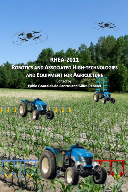
<strong>RHEA</strong>-2011<br />
ROBOTIICS AND ASSOCIIATED HIIGH-TECHNOLOGIIES<br />
AND EQUIIPMENT FOR AGRIICULTURE<br />
EEdi itted byy: :<br />
Pabl lo Gonzzal lezz--de--SSanttoss and Gi il ll less<br />
I<br />
Rabattel l
PROCEEDINGS OF THE FIRST INTERNATIONAL WORKSHOP ON<br />
ROBOTICS AND ASSOCIATED HIGH TECHNOLOGIES AND<br />
EQUIPMENT FOR AGRICULTURE<br />
(<strong>RHEA</strong>-2011)<br />
Montpellier, France<br />
September 9, 2011<br />
Edited by<br />
Pablo Gonzalez-de-Santos and Gilles Rabatel<br />
I
The research leading to these results has received funding from the European<br />
Union’s Seventh Framework Programme [FP7/2007-2013] under Grant Agreement<br />
nº 245986<br />
The views expressed in this document are entirely those of the authors and do not<br />
engage or commit the European Commission or the editors in any way.<br />
EDITORS<br />
ISBN: 978-84-615-6184-1<br />
Printed by Producción Gráfica Multimedia, PGM<br />
Rafael Alberti 14; 28400 Madrid, Spain<br />
Proceedings are available at: http://www.rhea-<strong>project</strong>.eu<br />
Pablo Gonzalez-de-Santos (CSIC-Centre for Automation and Robotics)<br />
Gilles Rabatel (Cemagref)<br />
CHAIR COMMITTEE<br />
Pilar Barreiro (Technical University of Madrid)<br />
Angela Ribeiro (CSIC-Centre for Automation and Robotics)<br />
Maria Guijarro (Complutense University of Madrid)<br />
Nathalie Gorretta (Cemagref)<br />
III
The <strong>RHEA</strong> consortium is formed by:<br />
Agencia Estatal Consejo Superior de Investigaciones Científicas (CSIC)<br />
(Coordinator)<br />
Spain<br />
(CSIC-CAR Centro de Automatica y Robotica<br />
(CSIC-ICA) Instituto de Ciencias Agrarias<br />
CSIC-IAS) Instituto de Agricultura Sostenible<br />
CogVis GmbH (CV)<br />
Austria<br />
Forschungszentrum Telekommunikation Wien Ltd. (FTW)<br />
Austria<br />
Cyberbotics Ltd (CY)<br />
Switzerland<br />
Università di Pisa (UP)<br />
Italy<br />
Universidad Complutense de Madrid (UCM)<br />
Spain<br />
Tropical (TRO)<br />
Greece<br />
Soluciones Agrícolas de Precisión S.L. (SAP)<br />
Spain<br />
Universidad Politécnica de Madrid (UPM)<br />
Spain<br />
UPM-EIA ETS Ingenieros Agrónomos<br />
UPM-EII ETS Ingenieros Industriales<br />
AirRobot GmbH & Co. KG (AR)<br />
Germany<br />
Università degli Studi di Firenze (UF)<br />
Italy<br />
Centre National du Machinisme Agricole, du Génie Rural, des Eaux et des<br />
Forêts -CEMAGREF (CE)<br />
France<br />
Case New Holland Belgium N.V (CNH)<br />
CNH-B Case New Holland Belgium N.V. Belgium<br />
CNH-F Case New Holland Belgium S.A. France<br />
Bluebotics S.A. (BL)<br />
Switzerland<br />
CM Srl (CM)<br />
Italy<br />
V
FOREWORD<br />
These proceedings are the result of the work developed by the <strong>RHEA</strong> consortium<br />
throughout the first year of the <strong>RHEA</strong> <strong>project</strong> (Robot fleets for highly effective<br />
agriculture and forestry management-FP7-NMP 245986). <strong>RHEA</strong> comprises a<br />
number of research centres, universities, and companies funded by the European<br />
Commission through the Seventh Framework Programme to develop robotic fleets<br />
for weed control and pesticide management in agriculture and forestry.<br />
In the planning stages of the workshop, researchers and engineers were invited to<br />
present ideas, research results, works in progress and system demonstrations<br />
related to robotics, perception and actuation for agricultural tasks. Associated<br />
technologies that allow these different techniques to be merged, such as<br />
communication, localisation and human-system interfaces, were also addressed.<br />
The objective of this workshop is to facilitate the dissemination of <strong>project</strong> results,<br />
but it also provides a forum for building community and motivating discussion, new<br />
insight and experimentation.<br />
This workshop was held in the pleasant city of Montpellier, France, on September<br />
9, 2011. It consisted of three sessions: (I) Weed Management, (II) Perception and<br />
analysis and (III) Specific Techniques for the <strong>RHEA</strong> Fleet. The editors appreciate the<br />
contributions of the speakers, authors and attendees to this first <strong>RHEA</strong> workshop,<br />
which can be considered a first step towards two International Conferences that<br />
will be arranged by the consortium in the coming years.<br />
Pablo Gonzalez-de-Santos and Gilles Rabatel<br />
VII<br />
Editors
VIII
CONTENTS<br />
Weed management<br />
A Five-Step Approach for Planning a Robotic Site-Specific Weed<br />
Management Program for Winter Wheat<br />
C. Fernández-Quintanilla, J. Dorado, C. San Martín, J. Conesa-<br />
Muñoz and A. Ribeiro<br />
Effect of thermal and mechanical weed control on garlic<br />
C. Frasconi, M. Fontanelli, M. Raffaelli, L. Martelloni and A.<br />
Peruzzi,<br />
Effect of flaming at different LPG doses on maize plants<br />
M. Fontanelli, C. Frasconi, M. Raffaelli, L. Martelloni and A.<br />
Peruzzi, 23<br />
Perception and analysis<br />
Hyperspectral imagery to discriminate weeds in wheat<br />
G. Rabatel, F. Ougache, N. Gorretta and M. Ecarnot<br />
Strategies for video sequence stabilization<br />
A. Ribeiro, N. Sainz-Costa, G. Pajares and M. Guijarro,<br />
How the spatial resolution can affect the quality of mosaics and<br />
assessment of optimum number of tie points necessary to obtain<br />
good quality images<br />
D. Gómez-Candón, S. Labbé, M. Jurado-Expósito, J. M. Peña-<br />
Barragán, G. Rabatel and F. López-Granados<br />
Camera System geometry for site specific treatment in precision<br />
agriculture<br />
M. Montalvo, J. M. Guerrero, M. Guijarro, J. Romeo, P. J.<br />
Herrera, A. Ribeiro and G. Pajares<br />
Techniques for Area Discretization and Coverage in Aerial<br />
Photography for Precision Agriculture employing mini quad-rotors<br />
J. Valente, D. Sanz, J. del Cerro, C. Rossi, M. Garzón, J. D.<br />
Hernández, and A. Barrientos<br />
Specific Techniques for the <strong>RHEA</strong> Fleet<br />
Analysis of Engine Thermal Effect on Electronic Control units for<br />
“Robot Fleets for Highly effective Agriculture and Forestry<br />
Management” (<strong>RHEA</strong>)<br />
M. Garrido, H. T. Jiménez-Ariza, M. A. Muñoz, A. Moya, C. Valero<br />
and P. Barreiro<br />
IX<br />
3<br />
13<br />
35<br />
47<br />
61<br />
73<br />
85<br />
101
Path-planning of a Robot Fleet Working in Arable Crops. First<br />
experiments and results<br />
A. Ribeiro and J. Conesa-Muñoz<br />
Simulation of communication within the <strong>RHEA</strong> robotic fleet<br />
M. Roca and S. Tomic,<br />
(Forschungszentrum Telekommunikation Wien - FTW)<br />
Safety functional requirements for “Robot Fleets for Highly effective<br />
Agriculture and Forestry Management” (<strong>RHEA</strong>)<br />
P. Barreiro, M. Garrido, A. Moya, B. Debilde, P. Balmer, J. Carballido,<br />
C. Valero, N. Tomatis and B. Missotten 141<br />
Application of mechanical and thermal weed control in maize as part<br />
of the <strong>RHEA</strong> <strong>project</strong><br />
A. Peruzzi, M. Raffaelli, M. Fontanelli, C. Frasconi and L. Martelloni,<br />
(Universita di Pisa)<br />
Wireless QoS-enabled Multi-Technology Communication for the <strong>RHEA</strong><br />
Robotic Fleet<br />
T. Hinterhofer and S. Tomic<br />
(Forschungszentrum Telekommunikation Wien - FTW)<br />
Vehicle Guidance on a Single-Board Computer<br />
M. Hödlmoser, C. Bober, M. Kampel and M. Brandstötter<br />
X<br />
117<br />
129<br />
159<br />
173<br />
187
A Five-Step Approach for Planning a Robotic Site-Specific Weed Management<br />
Program for Winter Wheat<br />
Weed Management<br />
1
A Five-Step Approach for Planning a Robotic Site-Specific Weed Management<br />
Program for Winter Wheat<br />
A Five-Step Approach for Planning a Robotic Site-Specific<br />
Weed Management Program for Winter Wheat<br />
Cesar Fernández-Quintanilla*, Jose Dorado*, Carolina San Martín*,<br />
Jesus Conesa-Muñoz** and Angela Ribeiro**<br />
�<br />
*Institute for Agricultural Sciences (CSIC), C/ Serrano 115B, 28006 Madrid, Spain<br />
(e-mail: cesar@ica.csic.es)<br />
**Centre for Automation and Robotics (UPM-CSIC), Crtra. Campo Real Km 0,2<br />
28500 Arganda del Rey, Madrid, Spain<br />
(e-mail: angela.ribeiro@csic.es)<br />
Abstract: A Five-Step procedure is proposed to be used in weed control programs<br />
based on the use of a robot fleet. The five steps are: 1) field inspection, 2) longterm<br />
decisions, 3) current year decisions, 4) unit distribution & path planning, and<br />
5) online decisions. Monitoring weed populations at various times could be<br />
achieved using unmanned aerial vehicles (UAV) equipped with cameras and GPS. A<br />
long-term decision module could be used to optimize the choice of crop and<br />
herbicide rotations as well as the tillage system. A computerized system should<br />
quickly query databases containing information about the weeds present in each<br />
field and the herbicides available to control them, performing calculations to<br />
determine the cost effectiveness of each option. The system should generate a<br />
georeferenced prescription map indicating the sites were each herbicide should be<br />
sprayed. This map should provide the information required to decide the optimal<br />
distribution of the spraying units of the fleet and their corresponding navigation<br />
plans. Final spraying decisions should be based on both, prescription maps and<br />
online information coming from sensors located in the sprayer.<br />
1. Introduction<br />
Weed control can be approached either on a hit or miss basis or as a carefully<br />
planned and coordinated program. The second alternative is most likely to yield<br />
success. A well planned program consists of a number of appropriate operations<br />
coordinated in a sequence. Various types of weed management programs have<br />
been devised to fit different types of situations (Clarke, 2002; Newman, 2002;<br />
Sheley et al., 2010).<br />
3
A Five-Step Approach for Planning a Robotic Site-Specific Weed Management<br />
Program for Winter Wheat<br />
Site-specific weed management is defined as the use of equipment embedded with<br />
technologies that detect weeds growing in a crop and, taking into account<br />
predefined factors such as economics, take action to maximize the chances of<br />
successfully controlling them (Christensen et al., 2009). Although several weed<br />
sensing systems and precision implements have been developed over the last two<br />
decades, several barriers still prevent the commercial implementation of these<br />
technologies. A reliable, high resolution weed detection system and a decision<br />
support system capable to integrate site-specific information on weed distribution,<br />
weed species composition and density and the effect on crop yield are decisive for<br />
an effective site-specific management (Christensen et al., 2009).<br />
Robotic weed control systems hold promise toward the automation of these<br />
operations and provide a means of reducing herbicide use. Although a few robotic<br />
weed control systems have demonstrated the potential of this technology in the<br />
field (Slaughter et al., 2008), additional research is needed to fully realize this<br />
potential.<br />
In this work, a Five-Step procedure has been proposed to be used in weed control<br />
programs based on the use of a robot fleet. The five steps are: 1) field inspection,<br />
2) long-term decisions, 3) current year decisions, 4) unit distribution & path<br />
planning, 5) online decisions. The outline structure of the system is shown in Fig. 1.<br />
Although the same structure can be used for a variety of crop situations, weed<br />
control tactics and local conditions, the system described in this paper has been<br />
developed for a concrete scenario: site-specific application of herbicides in winter<br />
wheat crops in Central Spain.<br />
4<br />
48-hr<br />
weather<br />
forecast<br />
WEEDS HERBICIDES<br />
Field inspection<br />
Data handling<br />
Long term decisions<br />
Current year decisions<br />
Path planning<br />
Online decisions<br />
AGRONOMY<br />
Rotation<br />
Tillage<br />
Herbicide<br />
Type of herbicide<br />
Dose of herbicide<br />
Timing of herbicide<br />
Unit distribution<br />
Path plan<br />
ON / OFF<br />
(site specific)<br />
Farmer`s<br />
knowledge<br />
Fig. 1. System architecture of <strong>RHEA</strong> Mission Planner for site-specific application of<br />
herbicides in wheat
2. Step 1: Field inspection<br />
Robotics and associated High technologies and Equipment for Agriculture<br />
Information on weed spatial distribution and abundance will be generated from<br />
aerial images obtained at different times prior to herbicide spraying and from<br />
information obtained from ground vehicles at spraying time. Aerial inspection of<br />
the fields in spring, when some broadleaved weeds are in full bloom (and can be<br />
easily discriminated from the crop) provide an excellent opportunity to<br />
discriminate and map infestations of selected weed species. Numerous studies<br />
have shown that detection of late-season weed infestation has considerable<br />
possibilities when the weeds exceed the crop canopy and the spectral differences<br />
between crops and weeds are maximum (López-Granados, 2011). Detection of<br />
bright coloured red poppies (Papaver rhoeas) on the green background provided by<br />
the crop may be a paradigmatic example of this situation. Monitoring weed<br />
populations at various times will be achieved using unmanned aerial vehicles<br />
(UAV). These vehicles provide high spectral, spatial and temporal resolutions with a<br />
relatively low cost (López-Granados, 2011). Additional georeferenced data on weed<br />
infestations will be obtained at spraying time by the cameras or sensors located on<br />
the sprayers (Andújar et al., 2011; Burgos-Artizzu et al., 2011).<br />
3. Step 2: Long-term decisions<br />
Farmers usually consider two different time-scales for decision making: long term<br />
(with a 3-5 year horizon) and current year. Consequently, a comprehensive system<br />
should include a long-term planning tool allowing users to consider various cultural<br />
practices (rotations, tillage systems) conducted over several years and a within<br />
season planning tool to investigate a range of weed control options in a single<br />
season (Parsons et al., 2009).<br />
The objective of the our long-term decision module is to optimize the choice of<br />
crop and herbicide rotations as well as the tillage system throughout a rotation (up<br />
to 5 years) defined by the user, trying to find the best long-term strategy. The<br />
decision process could be made using a finite horizon stochastic dynamic program,<br />
trying to identify the policy that maximizes the long term expected discounted<br />
return. Other option could be using a set of decision rules coupled with a rule<br />
editor and an inference engine. In order to take these decisions, different types of<br />
data are required.<br />
Historic maps, constructed using the weed distribution data obtained in the<br />
previous step, provide one major element for this process. In addition, empirical<br />
knowledge of the farmer, gathered through many years of working the field, is also<br />
a valuable data source that should be exploited, particularly when digital maps with<br />
historical records are not available. All this information is stored in a `Weed spatial´<br />
database.<br />
Biological data on the major weeds that are present in the field are required to<br />
assess the actual risks posed by those plants and the opportunities and possibilities<br />
5
A Five-Step Approach for Planning a Robotic Site-Specific Weed Management<br />
Program for Winter Wheat<br />
to manage them using different control tactics. Information on the life cycle,<br />
tendency to aggregate in patches, competitiveness with the crop, longevity of the<br />
seeds and possible beneficial effects to wildlife of all the major weed species<br />
present in winter wheat in Spain has been stored in a `Weed generic´ database (Fig.<br />
2).<br />
BROADLEAVED<br />
6<br />
Common names Present? Patchiness Competitiveness Longevity Beneficial<br />
Galium aparine Cleavers Medium High Low No<br />
Papaver rhoeas Poppy Low Medium Very high Yes<br />
Sinapis arvensis Wild mustard Medium High Medium Yes<br />
Veronica hedaerefolia Speedwell Low Low Medium No<br />
GRASSES<br />
Avena sterilis Wild oat High High Medium No<br />
Lolium rigidum Ryegrass Medium Medium Low No<br />
Bromus diandrus Rigput brome High High Low No<br />
Phalaris brachistachis Canarygrass High Medium Medium Yes<br />
Fig. 2. Example of a generic database with some of the major biological<br />
characteristics of selected weed species present in winter wheat crops in Spain.<br />
In the case of herbicides, a `Herbicide spatial´ database will be constructed using<br />
the prescription and spraying maps generated in previous years (in case the system<br />
is used over a series of years) as well as with information coming directly from the<br />
user (e.g. control failures in some zones of the field). A comprehensive `Herbicide<br />
generic´ data base with all the commercial herbicides available in Spain for winter<br />
wheat has been constructed. This database contains information on their optimal<br />
timing, weed selectivity, risk of resistance, toxicity, environmental effects, cost, etc.<br />
(Fig. 3).
1. Optimal growth stage:<br />
2. Weed selectivity:<br />
3. Other data:<br />
Robotics and associated High technologies and Equipment for Agriculture<br />
Tribenuron<br />
Dicamba<br />
Fluroxipir<br />
Diclofop<br />
Fenaxaprop<br />
Clodinafop<br />
Tribenuron<br />
Dicamba<br />
Fluroxipir<br />
Diclofop<br />
Fenaxaprop<br />
Clodinafop<br />
Fig. 3. Example of a generic database of selected herbicides for winter wheat<br />
Finally, the `Agronomy´ database will provide information on field size, boundaries<br />
and obstacles, cropping history, drilling and harvest dates, expected yields,<br />
expected crop value, basic costs for operations such as soil tillage, fertilizing and<br />
spraying as well as values for the variable costs associated with each crop. Although<br />
default values are provided by the system in some cases, in other cases they should<br />
be filled by the user.<br />
4. Step 3: Current year decisions<br />
1 leaf 2 leaves 3 leaves Early Medium Late Jointing<br />
tillering tillering tillering<br />
Broadleaved weeds Grasses<br />
Galium Papaver Sinapis Veronica Avena Lolium Phalaris<br />
Excellent<br />
Commercial<br />
Dose /ha<br />
product<br />
Aceptable<br />
Cost<br />
(€ / ha)<br />
Toxicity Wildlife risk<br />
Poor<br />
None<br />
Resistance<br />
group<br />
Tribenuron GRANSTAR 15-25 gr 20 Xi B B<br />
Dicamba BANVEL 0.3-0.5 l 10 Xi B O<br />
Fluroxipir STARANE 0.75-1 l 25 Xi - O<br />
Diclofop COLT 2.5 l 25 Xn B A<br />
Fenaxaprop PUMA 1.0-1.25 l 38 Xn A A<br />
Clodinafop TOPIK 0.17-0.35 g 40 Xn A A<br />
Weed management in conventional wheat production relies heavily on herbicide<br />
use. Current year decision-making for herbicide use is a complex task requiring the<br />
integration of information on weed biology, expected crop yields and potential<br />
yield losses caused by different weeds, herbicide options, timing and efficacy of<br />
each herbicide, economic profitability of the treatment and environmental risks<br />
(Fig. 4). Agricultural growers and consultants can manage the integration of these<br />
complex factors by using decision support systems (DSS) (Parsons et al., 2009).<br />
7
A Five-Step Approach for Planning a Robotic Site-Specific Weed Management<br />
Program for Winter Wheat<br />
48 h<br />
Weather<br />
forecast<br />
HERBICIDES WEEDS<br />
AGRONOMY<br />
Historic map<br />
DSS<br />
Path plan Herbicides<br />
required<br />
Prescription map<br />
Farmer`s<br />
knowledge<br />
Fig. 4. Outline structure of the major inputs and outputs involved in current year<br />
decisions<br />
The objective of the current year decision module is to suggest a range of different<br />
herbicides that result in good profits for the current season. The economic margin<br />
used considers both, the value of the wheat grain losses avoided by each treatment<br />
and the cost of that treatment. All the parameter values may be changed by the<br />
user. Optimization algorithms are used to assess each possible decision variable.<br />
Computer programs will be designed to facilitate this decision-making process. A<br />
computerized system should quickly query databases containing information about<br />
many different herbicide products, perform calculations to determine the cost<br />
effectiveness of each of them, and store detailed field records. The system will<br />
generate a georeferenced prescription map indicating the sites were each<br />
herbicide should be sprayed (Fig. 4). In addition, this map will provide the<br />
information required to adjust herbicide acquisition and loading the ground units<br />
to actual needs, to decide the optimal distribution of the spraying units of the fleet<br />
and their corresponding navigation plans.<br />
8
Robotics and associated High technologies and Equipment for Agriculture<br />
The final decision on field spraying depends heavily on weather conditions.<br />
Consequently, the system includes a set of decision rules based on the expected<br />
wind, temperatures and rainfall at treatment time and in the following 24 h (Fig. 4).<br />
5. Step 4: Unit distribution & path planning<br />
Numerous planning methods for obtaining the routes that allow an efficient<br />
operation of agricultural vehicles have been proposed (Stoll, 2003; Jin and Tang,<br />
2010; Taix et al., 2006). These methods take into account, for only one vehicle,<br />
different factors: the strategy of operation, the surrounding areas, the geometry of<br />
the field, field-specific data (size, slope, obstacles in the field), specific restriction<br />
on the machinery (p.e. turning radius), or the operation direction. The change of<br />
the direction in the headlands is an important issue because of the long time<br />
needed for this operation. Stoll (2003) has calculated the turning paths keeping in<br />
mind the effective width, the minimum turning radius, the driving speed and the<br />
turning acceleration of the vehicle. It also includes additional time to consider the<br />
change of the direction in the turning.<br />
Path planning taking into account the previous factors is a very complex process<br />
that requires rather sophisticated tools in order to search the optimal solution. The<br />
problem becomes even more complex when a fleet of robots is used to perform<br />
the herbicide treatment. The problem can be enunciated as follows (Conesa-Muñoz<br />
and Ribeiro, 2011): Given a set of robots with certain features (i.e., herbicide<br />
loading capacity, motion characteristics, width of the spraying boom), a field with<br />
specific dimensions, a crop growing in rows and a map of the weed patches, the<br />
aim is to find the subset of robots and associated paths that ensure the whole<br />
cover of the weed with the minimum cost (Fig. 5). The solution of this problem can<br />
be faced with a genetic algorithm approach where the fitness function considers<br />
several of the factors above explained (Conesa-Muñoz and Ribeiro, 2011).<br />
6 Step 5: Online decisions<br />
Although the prescription map provides basic information of the field areas that<br />
should be sprayed, this information needs to be contrasted with that obtained at<br />
spraying time with cameras or sensors that detect weed presence and discriminate<br />
different weed types. Once the detected weed patch has been considered as a<br />
suitable target for spraying, a fast-response controller will regulate discharge of the<br />
different herbicides in each individual nozzle (Fig. 6). Decision making could be<br />
made using a set of decision rules similar to those used in the long-term decision<br />
module.<br />
9
A Five-Step Approach for Planning a Robotic Site-Specific Weed Management<br />
Program for Winter Wheat<br />
Fig. 5. Distribution of three ground units to conduct a spraying operation following<br />
a predefined prescription map. Path plan for each individual unit marked with a<br />
different colour. Green cells indicate the presence of weeds. Circles indicate the<br />
starting position<br />
10<br />
Unit 1 Unit 2<br />
Online spraying<br />
Prescription map<br />
Genetic algorithms<br />
Fitness functions<br />
Prescription map<br />
Online detection<br />
Fig. 6. Online detection and spraying by a fast-response controller
Acknowledgement<br />
Robotics and associated High technologies and Equipment for Agriculture<br />
The research leading to these results has received funding from the European<br />
Union’s Seventh Framework Programme [FP7/2007-2013] under Grant Agreement<br />
nº 245986.<br />
References<br />
Andújar, D., A. Ribeiro, C. Fernández-Quintanilla and J. Dorado (2011). Accuracy<br />
and feasibility of optoelectronic sensors for weed mapping in row crops.<br />
Sensors 11, 2304-2318.<br />
Burgos-Artizzu, X.P., A. Ribeiro, M. Guijarro and G. Pajares (2011). Real-time image<br />
processing for crop/weed discrimination in maize fields. Computers and<br />
Electronic in Agriculture, 75, 337-346.<br />
Christensen, S., H.T. Sogaard, P. Kudsk, M. Norremark, I. Lund and E.S. Nadimi<br />
(2009). Site-specific weed control technologies. Weed Research, 49, 233-241.<br />
Clarke, J. (2002). Weed management strategies for winter cereals. In: Weed<br />
Management Handbook (R.E.L. Naylor, Ed.), pp. 354-358. Blackwell Science<br />
Ltd. for British Crop Protection Council, Oxford, UK.<br />
Conesa-Muñoz, J. and A. Ribeiro (2011). An evolutionary approach to obtain the<br />
optimal distribution of a robot fleet for weed control in arable crops. In:<br />
EFITA/WCCA '11: 8th European Federation for Information Technology in<br />
Agriculture, Food and the Environment Congress/Word Congress on Computers<br />
in Agriculture (E. Gelb and K. Charvát, Eds.), pp. 141-155. Czech Centre for<br />
Science and Society, Prague, Czech Republic.<br />
Jin, J. and L. Tang (2010). Optimal coverage path planning for arable farming on 2D<br />
surfaces. Transactions of the ASABE, 53, 283-295.<br />
López-Granados, F. (2011). Weed detection for site-specific weed management:<br />
mapping and real-time approaches. Weed Research 51, 1-11.<br />
Newman, J.R. (2002). Management of aquatic weeds. In: Weed Management<br />
Handbook (R.E.L. Naylor, Ed.). Pp. 399-414. Blackwell Science Ltd. for British<br />
Crop Protection Council, Oxford, UK.<br />
Parsons, D.J., L.R. Benjamin, J. Clarke, D. Ginsburg, A. Mayes, A.E. Milne and D.J.<br />
Wilkinson (2009). Weed Manager-A model-based decision support system for<br />
weed management in arable crops. Computers and Electronics in Agriculture,<br />
65, 155-167.<br />
Sheley, R.L., J.J. James, B.S. Smith and E.A. Vasquez (2010). Applying ecologically<br />
based invasive-plant management. Rangeland Ecology and Management, 63,<br />
605-613.<br />
Slaughter, D.C., D.K. Giles and D. Downey (2008). Autonomous robotic weed<br />
control systems: A review. Computers and Electronics in Agriculture, 61, 63-78.<br />
11
A Five-Step Approach for Planning a Robotic Site-Specific Weed Management<br />
Program for Winter Wheat<br />
Stoll, A. (2003). Automatic operation planning for GPS-guided machinery. In:<br />
Precision Agriculture ’03 (J.V. Stafford and A. Werner, Eds.), pp. 657-664.<br />
Wageningen Academic Publishers, Wageningen, The Netherlands.<br />
Taïx, M., P. Souères, H. Frayssinet and L. Cordesses (2006). Path planning for<br />
complete coverage with agricultural machines field and service robotics. In:<br />
Field and Service Robotics (S. Yuta, H. Asama and S. Thrun, Eds.), pp. 549-558.<br />
Springer Tracts in Advanced Robotics, Vol. 24. Berlin, Germany.<br />
12
A Five-Step Approach for Planning a Robotic Site-Specific Weed Management<br />
Program for Winter Wheat<br />
Effect of thermal and mechanical weed control on garlic<br />
Christian Frasconi, Marco Fontanelli, Michele Raffaelli, Luisa Martelloni and<br />
Andrea Peruzzi<br />
�<br />
CIRAA “E. Avanzi”, University of Pisa, Via Vecchia di Marina 6, 56010 S. Piero a<br />
Grado PI, Italy<br />
(e-mail: cfrasconi@agr.unipi.it)<br />
Abstract: Vessalico is a small village close to Imperia (Liguria, Italy), where garlic is a<br />
typical crop. The garlic of Vessalico is one of the most traditional and top quality<br />
foods in Italy. A study was carried out on the possibility of introducing a<br />
mechanization chain to solve the main agronomic problems of garlic cultivation in<br />
this area, such as planting, weed control and harvesting, which would thus improve<br />
garlic yield and quality. Ordinary organic garlic crop management was compared<br />
with an innovative system in which physical weed control was carried out using a<br />
rolling harrow, two flame weeding machines and a precision hoe. The innovative<br />
treatments increased the whole plant and bulb dry weight by approximately 38%<br />
and 78% respectively, and reduced weed biomass at harvest by up to 77%.<br />
1. Introduction<br />
Vessalico is a village (Latitude 44°3 N, Longitude 7°58’ E) in the district of Imperia,<br />
Liguria, NW Italy. The farms in this area are very small, and crops are grown in small<br />
terraced plots. As a result, operative machines must be easy to handle and not<br />
cumbersome. Garlic is the main crop in this area, it is sold as a dried or processed<br />
high quality product, and is famous worldwide. Furthermore all the garlic<br />
cultivation in the area is organic, which provides added value to the crop. The<br />
division of Agriculture Engineering and Farm Mechanization Department of<br />
Agronomy and Agro-Ecosystem Management and the Centro Interdipartimentale di<br />
Ricerche Agro-Ambientali “Enrico Avanzi” of the University of Pisa, in collaboration<br />
with the Agriculture and Civil Defence department of Liguria and the “A Resta”<br />
Cooperative of farmers carried out a study on the possibility of introducing a<br />
mechanization chain to solve the main agronomic problems involved in the<br />
cultivation of garlic in this area, such as planting, weed control and harvesting,<br />
which would thus improve garlic yield and quality (Peruzzi et al. 2007).<br />
13
Effect of flaming with different LPG doses on maize plants<br />
2. Materials and methods<br />
The study was carried out in 2006-2007 in Vessalico (Imperia, Italy). The traditional<br />
organic garlic farming system was compared with an innovative system.<br />
2.1 The traditional farming system<br />
The farmers of Vessalico usually plant bulbs using a “one row” potato planter (Fig.<br />
1), modified for garlic. This equipment reduces working time compared to hand<br />
sowing, however it places the bulbs very deep in the soil, making it difficult for the<br />
plants to emerge.<br />
14<br />
Fig. 1. Modified single row potato planter used in the traditional farm system of<br />
Vessalico for planting garlic<br />
The usual inter-row space is 50 cm. Weed control is carried out with a selfpropelled<br />
cultivator (Fig. 2) between the rows, and by hand in the row. This<br />
technique is very expensive and can damage the garlic root system if the treatment<br />
is performed in a late phenological crop stage.<br />
Fig. 2. Self-propelled cultivator used for inter-row weed control in the traditional<br />
farm system of Vessalico
Robotics and associated High technologies and Equipment for Agriculture<br />
2.2 The innovative farming system<br />
In the innovative system, three different machines, each 1.4 m wide, were used for<br />
physical weed control: a rolling harrow, two flamers and a precision hoe.<br />
2.3 Rolling harrow<br />
The rolling harrow is equipped with specific tools (Fig. 3: spike discs placed at the<br />
front, and cage rolls mounted in the rear. The front and rear tools are connected by<br />
an overdrive with a ratio equal to 2. The disc and the rolls can be placed differently<br />
on the axles: in close arrangement, in order to create a very shallow tillage (3-4 cm)<br />
of the whole treated area (for seedbed preparation and non-selective weed control<br />
after false seed bed) and in a spaced arrangement, in order to create efficient<br />
selective post emergence weed control (for precision inter-row weeding) (Peruzzi,<br />
2005 and 2006).<br />
Fig. 3. The rolling harrow: close arrangement for full surface treatment (top);<br />
spaced arrangement for inter row treatment (down)<br />
2.4 Flaming machines<br />
The mounted flamer (Fig. 4) is an open flame machine equipped with three LPG 50<br />
cm wide rod burners. The machine has a “thermal exchanger”, which consists in a<br />
hopper containing water heated by the exhaust gas of the tractor engine. Each<br />
burner is placed on a wheeled articulated parallelogram in order to maintain the<br />
correct distance from the soil surface. In the experimental field trials, the machine<br />
15
Effect of flaming with different LPG doses on maize plants<br />
was used for crop emergence treatment with a driving speed of about 3 km h -1 and<br />
different LPG pressures. During the trials, a hand flamer, equipped with a 15 cm<br />
wide rod burner was also used by a walking operator at a LPG pressure of 0.2 MPa<br />
and average speed of 2 km h -1 .<br />
16<br />
Fig. 4. Mounted flaming machines used during the study in Vessalico<br />
2.5 Precision hoe<br />
The precision hoe is equipped with a hand guidance system and six working units<br />
connected to the frame by articulated parallelograms (Fig. 5). Each unit has a 9 cm<br />
wide horizontal blade and two sets of tools (spring tines suitable as vibrating tines<br />
and a torsion weeder) in order to perform both inter and intra row weed control<br />
(Fig. 6).<br />
2.6 The experimental trial<br />
Our weed control strategy consisted in creating a false seedbed with a rolling<br />
harrow, followed by flaming after crop emergence. This is because garlic can<br />
tolerate exposure to thermal radiation for a few tenths of second. Flaming or<br />
precision hoeing were used for further weed control . Harvesting was carried out<br />
manually for both systems. This is because the garlic plants are dried with whole<br />
leaves, in order to twist them into the traditional strings. During the experimental<br />
trials, physical weed control treatments were carried out separately. Firstly, a false<br />
seed bed was created with the rolling harrow on each experimental plot.<br />
Subsequently, garlic was sown manually in three rows spaced 20 cm apart. At early<br />
post emergence, flame weeding was carried out at different working pressures<br />
(0.2; 0.3; 0.4; 0.5 MPa) using a 3 km h -1 driving speed. At the four leaf stage, three<br />
different secondary treatments for each working pressure were performed:
Robotics and associated High technologies and Equipment for Agriculture<br />
precision hoeing with vibrating tines + torsion weeder, precision hoeing + torsion<br />
weeder and manual flaming carried out with a device carried on the operator's<br />
back and operating at a speed of about 2 km h -1 and a working pressure of 0.2 MPa.<br />
On some experimental plots, no secondary treatment was performed. Weed interrow<br />
and intra-row densities were determined on the basis of a 25×30 cm sampling<br />
area. At harvest, crop production and weed biomass were determined. The<br />
experimental design was a strip plot with three replicates. Data were analysed by<br />
ANOVA. Treatment means were separated using Fisher's least square difference at<br />
P< 0.05 (Gomez and Gomez 1984)<br />
Fig. 5. The six-element precision hoe: A) seat for the operator; B) hand guidance<br />
system; C) directional wheel; D) articulated parallelogram; E) horizontal blade; F)<br />
lateral disc; G) wheel of the articulated parallelogram; H) spring tines<br />
Fig. 6. The precision hoe spring tools: vibrating tines (left); torsion weeder (right)<br />
17
Effect of flaming with different LPG doses on maize plants<br />
3. Results<br />
Data collected 29 days after the first thermal treatment showed that the most<br />
efficient working pressure in controlling inter-row weeds was 0.3 MPa (Fig. 7).<br />
Weed density recorded 35 days after the secondary treatment revealed significant<br />
differences between the treated and untreated plots, but no significant differences<br />
were observed between the different secondary performed operations (Fig. 8). The<br />
weed flora percentage reduction ranged from 24% to 57%.<br />
Fig. 7. Effects of the different flame weeding working pressures on weed density 29<br />
days after the treatment. Different letters within bar of the same color indicate<br />
statistically significant differences (LSD P� 0.05)<br />
Significantly higher total dry weights and bulb dry weights were observed using a<br />
working pressure of 0.2 MPa (fig. 9). No significant differences were observed<br />
between the secondary treatments. Comparing results obtained in the<br />
experimental plots flamed at a working pressure of 0.2 MPa, with those obtained in<br />
plots managed traditionally, a significantly higher yield in terms of total and bulb<br />
dry weight (Fig. 10), and a significant lower value of weed dry biomass at harvest<br />
were observed (Fig. 11).<br />
4. Discussion<br />
Weed control is the main agronomic problem of garlic in this area. Flame<br />
weeding seems to result in good weed control. The working pressure of 0.3 MPa<br />
18
Robotics and associated High technologies and Equipment for Agriculture<br />
Fig. 8. Effect of the different secondary treatments on weed density : S1) Precision<br />
hoeing with torsion weeder; S2) Precision hoeing with vibrating tines and torsion<br />
weeder; P) Flame weeding; T) No treatment. Different letters within bar of the<br />
same color indicate statistically significant differences (LSD P� 0.05)<br />
Fig. 9. Effects of the different flame weeding working pressures on garlic yield days<br />
after the treatment. Different letters within bar of the same color indicate<br />
statistically significant differences (LSD P� 0.05)<br />
19
Effect of flaming with different LPG doses on maize plants<br />
20<br />
Fig. 10. Data of estimated garlic yield of our weed control strategy and the<br />
traditional system adopted by the farm. Different letters within bar of the same<br />
color indicate statistically significant differences (LSD P� 0.05)<br />
Fig. 11. Data of estimated garlic yield of the innovative weed control strategy and<br />
the traditional system adopted by the farm. Different letters within bar of the<br />
same color indicate statistically significant differences (LSD P� 0.05)<br />
ensured the best weed control results in terms of plant density. The working<br />
pressure of 0.2 MPa gave the highest yield and good control of the weed flora,<br />
compared with traditional weeding.
Robotics and associated High technologies and Equipment for Agriculture<br />
These results can be simply explained by considering that the use of increasing<br />
pressure (without any change in speed) resulted in a increase in heat transmission<br />
both to the weeds and crops. This higher pressure resulted in a higher degree of<br />
weed control, but lead to a decrease in garlic yield, while a pressure of 0.2 MPa<br />
seemed to represent the best compromise.<br />
5. Conclusions<br />
The introduction of a mechanization chain in organic garlic in Vessalico seems<br />
feasible, using machines already available on the market with modifications where<br />
necessary. Regarding weed control, the experimental trials carried out using the<br />
equipment designed at the University of Pisa showed interesting results that could<br />
lead to a more precise definition of the best strategy for these environments.<br />
Acknowledgement<br />
The research leading to these results has received funding from the European<br />
Union’s Seventh Framework Programme [FP7/2007-2013] under Grant Agreement<br />
nº 245986.<br />
References<br />
Gomez K.A., Gomez A.A. (1984) Statistical procedures for agricultural research II<br />
edition. Eds John Wiley & Sons U.S.A.<br />
Peruzzi A. (2005): La gestione fisica delle infestanti su carota biologica e su altre<br />
colture tipiche dell’altopiano del Fucino. Stamperia Editoriale Pisana Agnano<br />
Pisano (PI).<br />
Peruzzi A. (2006): Il controllo fisico delle infestanti su spinacio in coltivazione<br />
biologica ed integrata nella Bassa Valle del Serchio. Stamperia Editoriale Pisana<br />
Agnano Pisano (PI).<br />
Peruzzi A., Raffaelli M., Ginanni M., Fontanelli M., Lulli L., Frasconi C. (2007): La<br />
Meccanizzazione dell’Aglio di Vessalico. Proceedings of Convegno Nazionale III<br />
V e VI Sezione AIIA Pisa-Volterra 5-7 settembre 2007 “Tecnologie innovative<br />
nelle filiere: orticola, vitivinicola e olivicolo-olearia.” p. 120-123.<br />
21
A Five-Step Approach for Planning a Robotic Site-Specific Weed Management<br />
Program for Winter Wheat<br />
Effect of flaming with different LPG doses on maize plants<br />
Marco Fontanelli, Christian Frasconi, Luisa Martelloni, Michele Raffaelli and<br />
Andrea Peruzzi<br />
�<br />
*Centro Interdipartimentale di Ricerche Agro-Ambientali “Enrico Avanzi”, via<br />
Vecchia di Marina 6, 56122, San Piero a Grado, Pisa, Italy<br />
(e-mail: mfontanelli@agr.unipi.it).<br />
Abstract: Despite now being considered as a very innovative technique, the use of<br />
flaming for weed control is an old tradition. It was very common in the USA until<br />
the 1960s, when herbicides were still not very popular. After several decades,<br />
interest has been renewed in the USA, Canada and Europe, because of increasing<br />
environmental and health concerns. Flaming can be used to control weeds before<br />
crop planting/emergence (non-selective) and after crop emergence (selective).<br />
In this context, a specific machine for mechanical-thermal weed control in maize is<br />
being developed within the European Project <strong>RHEA</strong>. This machine will provide<br />
selective thermal in-row weed control and mechanical between-row weed<br />
removal.<br />
This paper focuses on thermal weed control and reviews some of the studies that<br />
describe the tolerance of maize to flaming. The yield loss is generally very low and<br />
the treatment does not greatly affect the production, especially with doses lower<br />
than or equal to 50 kg ha -1 . The maximum threshold is generally not higher than 15-<br />
20% of yield loss and is usually reached just with doses higher than 100 kg ha -1 .<br />
1. Introduction<br />
Public concern regarding agrochemical issues is constantly increasing (Ascard et al.<br />
2007). This is probably one of the most important reasons for the great diffusion of<br />
alternative/integrated/organic farming systems in Europe and North America<br />
(IFOAM et al. 2009, Ulloa, Datta and Knezevic 2010b, van der Weide et al. 2008).<br />
The European organic food market grew from about twelve thousand million euros<br />
in 2005 to eighteen thousand million in 2008 (IFOAM et al. 2009). There was a<br />
considerable increase in organic areas in Europe between 2005 and 2008, with<br />
cereals and fodders as the main crops (Eurostat, Press and Office 2010). In addition<br />
severe EU Directives and Regulations are having a big impact on farmers' choices<br />
for an environmental-friendly/sustainable agriculture. There has recently been a<br />
substantial reduction in the number of the active ingredients available (the ones<br />
considered potentially dangerous by the EU Commission), and probably many other<br />
products are about to be banned by the EU (EU/Directive 1991, DIRECTIVE 2009,<br />
REGULATION 2009). Farmers are encouraged to use “integrated pest management<br />
23
Effect of flaming with different LPG doses on maize plants<br />
means” and “sustainable, biological, physical and non-chemical methods must be<br />
preferred to chemical methods if they provide satisfactory pest control” (DIRECTIVE<br />
2009).<br />
Weed control has always been a major problem in agriculture and probably is the<br />
biggest in organic farming systems (Bàrberi, 2002). The only solution for organic<br />
farmers is to use mechanical and thermal means. Mechanical weed control consists<br />
in using soil tillage, and cutting and extracting/pulling weeds (Cloutier et al., 2007).<br />
Thermal weed control involves different kinds of radiation (i.e. fire, flaming, hot<br />
water, steam) in order to cause thermal injury to the weeds (Ascard et al. 2007).<br />
Therefore a “holistic” approach is generally the most advisable way to provide an<br />
efficient non-chemical weed management. The integration of preventive, cultural<br />
and direct means is often the only solution for satisfying and remunerative crop<br />
production (Bàrberi, 2002, Bond and Grundy, 2001). A hot topic in weed science<br />
and agricultural engineering is the study of mechanical and thermal means for nonchemical<br />
weed management, along with research into new types of machines for<br />
non-chemical weed control (Cloutier et al., 2007, Ascard and van der Weide, 2011).<br />
This paper focuses on flame weeding, which is the most widely used thermal<br />
control method (Ascard et al., 2007), and its application to maize, as a selective<br />
post-emergence treatment (Ulloa et al., 2011). A review of some of the studies<br />
carried out to investigate the maize response to heat is presented, since an<br />
innovative autonomous machine will be built within the <strong>RHEA</strong> <strong>project</strong> for<br />
mechanical-thermal weed control in maize. This machine will provide mechanical<br />
weed control between the rows and selective thermal weed control in the row. For<br />
further information please see the specific work in the proceedings of this<br />
workshop.<br />
2. Flaming: the general and “historical” background<br />
Flaming consists of the use of an open flame to control weeds. This method does<br />
not leave any residue either in the soil, the water or the crop, and it is acceptable<br />
practice in organic agriculture (Ascard et al., 2007).<br />
The principle is based on heating up the cells of the plant, which causes the<br />
denaturation and aggregation of cellular proteins and protoplast expansion and<br />
rupture. The final result is the desiccation of the upper part of the plant, but the<br />
roots are not injured. Depending on the stage and the type of plant, several<br />
treatments may be required as shoots may regenerate (Ascard et al., 2007,<br />
Vanhala et al., 2004).<br />
Large-scale flaming was used between 1940-1960 mainly for selective post<br />
emergence applications (Ascard et al., 2007). The first flame weeder was developed<br />
in the USA in 1852, and numerous machines were patented thereafter. Initially the<br />
24
Robotics and associated High technologies and Equipment for Agriculture<br />
main purpose of these machines was to destroy insects. Afterwards flaming was<br />
mainly used for weeds. In Australia flaming was used in the early 1930s for weed<br />
control in sugar cane without injuring the crop. In 1935 it was used for the first<br />
time in cotton fields. In 1941 flaming was successfully applied in Louisiana on sugar<br />
cane, and 10 flaming machines were constructed and used in 1943 (de Rooy, 1992).<br />
In 1945 LPG (liquefied petroleum gas, mainly propane and butane) equipment was<br />
introduced for farm use ,and replaced liquid fuels such as kerosene and oils (de<br />
Rooy, 1992, Ascard et al., 2007). With the introduction of LPG, a completely<br />
different technology was developed. It was a tough task for agricultural engineering<br />
research (de Rooy, 1992). Flaming was then widely used in the USA until the mid<br />
1960s in cotton, maize soybeans, lucerne, potatoes, onions, grapes, blueberries<br />
and strawberries (Ascard et al., 2007). Because of the increase in the cost of petrol<br />
and the development of the agrochemical industry, flaming became less popular in<br />
the USA in the 1970s (Ascard et al., 2007).<br />
Interest in this technique in USA and Canada has been renewed because of public<br />
concern regarding agrochemicals (Ascard et al., 2007, Bruening et al., 2009,<br />
Domingues et al., 2008, Knezevic et al., 2009a, Knezevic, Datta and Ulloa 2009b,<br />
Knezevic et al., 2009c, Knezevic and Ulloa 2007, Teixeira et al., 2008). In Europe<br />
flaming was not popular in the 1960s. Subsequently it became more widely used<br />
for organic farming systems and was first adopted in Germany and Switzerland<br />
(Ascard et al. 2007). Flaming is still quite common in Europe for organic farming<br />
systems, especially in seeded horticultural crops, and research into physical and<br />
cultural weed control is currently being carried out (Ascard, 1990, Ascard and van<br />
der Weide 2011, Vanhala et al., 2004, Peruzzi et al., 2007, Raffaelli et al., 2010,<br />
Raffaelli et al., 2011).<br />
There are two main groups of LPG burners for weed control: the liquid or self<br />
vapourizing type, and the vapour type (Ascard et al., 2007, de Rooy, 1992). In the<br />
first type, the LPG is liquid from the tank to the burner and is vapourized into gas<br />
when it reaches the burner. In the second group, LPG is already in the gas phase<br />
when drawn from the tank (de Rooy, 1992). This second group generally requires a<br />
heat exchange system to avoid the tank freezing because of the high energy<br />
requirement of the LPG passing from the liquid to the gas phase (Peruzzi et al.,<br />
2007, Raffaelli et al., 2010, Raffaelli et al., 2011).<br />
The shape of the burner and the flame can be flat or tubular. Burners can be open<br />
or covered by a specific hood. This second option is generally used for nonselective<br />
flaming before crop emergence, for weed control in urban areas and for<br />
haulm destruction (Ascard et al., 2007). The burner should be set appropriately in<br />
order to avoid flame deflection. Generally the angle of the burner should be around<br />
45°, with a ground clearance of about 10 cm (Ascard et al., 2007). One of the most<br />
common is the Hoffmann burner, which was developed in Germany. It is shaped<br />
like a rod and provides a stable and controllable flame (Ascard et al., 2007, de<br />
25
Effect of flaming with different LPG doses on maize plants<br />
Rooy, 1992). For a common open flamer, LPG consumption, usually varies from 20<br />
to 50 kg ha -1 (Ascard et al., 2007, Peruzzi et al., 2007, Raffaelli et al., 2010, Raffaelli<br />
et al., 2011).<br />
3. Flaming: when and where it can be used<br />
Flaming can be applied:<br />
Before crop planting/emergence on the whole surface (non-selective broadcast<br />
flaming). This method obviously does not require a heat tolerant crop.<br />
After crop emergence:<br />
Non-selective flaming between rows (does not require a heat tolerant crop)<br />
Selective flaming. These methods require heat tolerant crops:<br />
Broadcast flaming (the whole surface area where the crop is located is flamed)<br />
Burners are placed in the rows<br />
Burners are directed at the collar of the crop (“cross flaming”) (Fig. 1)<br />
Non selective flaming before crop planting/emergence is very common in organic<br />
farming with the false seedbed technique, which provides preventive weed control<br />
through seedbank depletion. Weed emergence is stimulated by a delayed seedbed<br />
preparation and the last phase before crop emergence is carried out by flaming.<br />
This does not disturb the soil and the emerging crop and does not stimulate further<br />
weed emergence. This technique is very common in low competitive vegetable<br />
production (i.e. carrot) and is combined with post-emergence mechanical weed<br />
control (Peruzzi et al., 2007, Raffaelli et al., 2010, Raffaelli et al., 2011, Ascard and<br />
van der Weide, 2011).<br />
Non-selective flaming after crop emergence between rows was developed in the<br />
1960s in the USA for weed and insect control in many crops, and for potato haulm<br />
desiccation (Ascard et al., 2007). However this application is not common as a<br />
cultivator/hoe provides less energy-consuming weed control between rows.<br />
Selective broadcast flaming provides weed control on the whole surface where the<br />
crop is located. Heat tolerant crops are required such as maize and onions (Ascard<br />
et al., 2007). Several successful trials were carried out at the University of<br />
Nebraska, in order to investigate the responses of maize, sweet maize, popcorn,<br />
soybean, sorghum, and wheat to broadcast flaming (Ulloa et al., 2011, 2010a,<br />
2010b, 2010c).<br />
Intra-row weed control is challenging for organic farming systems because it is<br />
often very labour intensive, especially in vegetable crops (Fogelberg, 2007, van der<br />
Weide, et al. 2008). This is why in-row flaming plus between row cultivation is a<br />
good option in order to reduce LPG consumption and crop injury compared to<br />
26
Robotics and associated High technologies and Equipment for Agriculture<br />
broadcast flaming (Peruzzi et. al., 2000, Knezevic et al., 2011). LPG consumption is<br />
lower as the treatment is performed in bands. Crop injury can be reduced by<br />
choosing a “cross” adjustment of the burners. Two burners are placed on each row,<br />
perpendicular to the driving direction and directed at the lower part of the stem,<br />
which is more resistant than the higher part (Ascard et al., 2007). This option was<br />
chosen for the <strong>RHEA</strong> <strong>project</strong>.<br />
4. Is maize really resistant to flaming?<br />
The effect of flame weeding on maize has been widely studied since the 1940s (de<br />
Rooy, 1992):<br />
“Flame weeding is a matter of differential burning. Just enough heat should be<br />
applied to kill the weeds, but not enough to kill the crop plants. Some crop plants,<br />
such as corn, have more resistance to flame than do the common weeds;<br />
therefore, corn is flamed successfully (Wright, 1947 cited in de Rooy 1992).”<br />
Research on flaming in maize were carried out in the USA in the 1960s. In 1969<br />
flaming was tested for the first time before crop emergence with the “delayed<br />
seeding technique” (de Rooy, 1992). Specific experiments on selective flaming were<br />
carried out in maize when the crop was about 30 cm tall. The results showed that<br />
flaming should be used in combination with other methods such as mechanical<br />
hoeing or cultivation.<br />
Guidelines provided by Hoffman specify that maize should be flamed up to 25 cm<br />
tall (de Rooy, 1992). His burner was improved by Lincoln University in New Zealand<br />
in the 1990s (de Rooy, 1992).<br />
Fig. 1. Cross flaming, and the test bench developed by the University of Pisa<br />
(Peruzzi et al., 2000)<br />
Laboratory and field trials carried out in Canada showed that maize can tolerate<br />
two different treatments at the 2-3 leaf and 6-7 leaf stages without a significant<br />
reduction in yield. An intermediate treatment at the 4-5 leaf stage was not<br />
advisable as it resulted in a considerable reduction in yield (Leroux et al., 2001).<br />
27
Effect of flaming with different LPG doses on maize plants<br />
Table 1. The effect of LPG dose on maize dry grain as affected by the growth stage<br />
of flaming (Peruzzi et al., 2000). Different letters indicate significant differences at<br />
LPG Consumption<br />
(kg/ha)<br />
28<br />
Stage<br />
P < 0.05 (Duncan’s Multiple Range Test)<br />
Maize dry grain per plant (g)<br />
1-2 leaves 4 leaves 8 leaves<br />
7,24 103.8 abc 108.9 abcd 111.7 a<br />
9,31 98.1 abc 125.9 abc 117.3 a<br />
11,96 96.8 abc 107.9 abcd 103.8 ab<br />
13,04 112.1 abc 129.3 abc 120.4 a<br />
15,37 95.6 abc 117.1 abc 122.8 a<br />
17,02 123.3 abc 109.1 abcd 116.4 a<br />
21,70 122.2 abc 113.0 abcd 114.4 a<br />
21,89 124.0 ab 108.6 abcd 110.1 ab<br />
22,22 93.4 bc 99.7 cd 100.4 ab<br />
25,52 95.1 bc 132.6 a 129.9 a<br />
28,57 88.5 c 102.4 abcd 102.3 ab<br />
30,64 100.4 abc 111.8 abcd 108.5 ab<br />
35,80 120.0 abc 106.8 abcd 116.5 a<br />
40,00 88.6 c 104.8 abcd 81.9 b<br />
51,07 95.7 abc 110.3 abcd 103.1 ab<br />
65,20 130.2 a 130.3 ab 117.3 a<br />
66,67 88.8 c 100.8 bcd 82.7 b<br />
107,60 130.3 a 132.7 a 115.4 a<br />
153,20 96.3 abc 116.0 abcd 106.9 ab<br />
200,00 89.9 bc 85.8 d 82.1 b<br />
Control 110.4 abc 110.4 abcd 110.4 ab
Robotics and associated High technologies and Equipment for Agriculture<br />
At the University of Pisa, we carried out laboratory experiments on selective “cross<br />
flaming” in maize using a 25 wide rod open flame burner (Fig. 1). Different<br />
combinations of LPG pressures and working speeds were tested, resulting in a<br />
different LPG consumption ha -1 (total amount of LPG per ha, whose dosage did not<br />
correspond to the actual dose on the row-band) from 7 to 200 kg ha -1 (Tab. 1). No<br />
statistically significant yield reductions were observed with any of the tested doses<br />
and at any growth stage (Peruzzi et al., 2000). For example, the yield loss observed<br />
with an LPG consumption of about 50 kg ha -1 was just 7%. The average yield loss<br />
obtained using the highest LPG consumption ha -1 (200 kg) was about 20%.<br />
Recent studies carried out by the University of Nebraska (USA) on broadcast<br />
flaming in maize partially contradict the results previously reported by Leroux and<br />
colleagues (2001), as V5 stage had in this case the least yield loss followed by V7<br />
and V2 (maximum yield losses of 3%, 11% and 17% obtained with the highest<br />
propane dose 85 kg ha -1 respectively). A yield reduction of about 12%, 8% and 3%<br />
were observed at V2, V7 and V5 stages respectively, with a propane dose from 45<br />
up to 55 kg ha -1 (Ulloa et al., 2011). Further experiments have been carried out by<br />
the same research group in order to test a combined flaming-cultivation treatment<br />
in maize. Results of just the first year showed that this kind of treatment should be<br />
preferably performed twice, at V3 and V6 stages (Knezevic et al., 2011).<br />
5. Conclusions<br />
The <strong>RHEA</strong> <strong>project</strong> will lead to the development of a new machine for combined<br />
thermal-mechanical weed control treatments in maize. Flaming will be performed<br />
selectively in rows. The flames will be targeted at the base of the crop. The actual<br />
in-row doses will vary from about 45 kg ha -1 to about 55 kg ha -1 , which corresponds<br />
to a maximum LPG consumption of less than 20 kg ha -1 , if the treatment is<br />
performed on all the surface.<br />
Based on the results from recent research on maize, the mechanical-thermal<br />
treatment could be repeated twice with the recommended doses, without<br />
significantly affecting the maize yield. As the flaming dose is strictly related to the<br />
type of burner, the effects of flaming on maize and weeds using the new burners<br />
will be investigated at the University of Pisa specifically for the <strong>RHEA</strong> <strong>project</strong>.<br />
Acknowledgement<br />
The research leading to these results has received funding from the European<br />
Union’s Seventh Framework Programme [FP7/2007-2013] under Grant Agreement<br />
nº 245986.<br />
References<br />
Ascard, J. (1990). Thermal weed control with flaming in onions. Proceedings 3rd<br />
International Conference IFOAM, Non-Chemical Weed Control, 34, 175-188.<br />
29
Effect of flaming with different LPG doses on maize plants<br />
Ascard, J., P. E. Hatcher, B. Melander and M. K. Upadhyaya (2007). Thermal weed<br />
control. Non-chemical Weed Management, 155-175.<br />
Ascard, J. and R. Y. van der Weide. (2011). Thermal weed control with the focus on<br />
flame weeding. In Physical weed control: Progress and challenges, eds. D. C.<br />
Cloutier & M. L. Leblanc, 71-90. Pinawa, Manitoba, Canada R0E 1L0: Canadian<br />
Weed Science Society - Société canadienne de malherbologie.<br />
Bàrberi, P. (2002). Weed management in organic agriculture: are we addressing the<br />
right issues? Weed research, 42, 176-193.<br />
Bond, W. and A. C. Grundy (2001). Non-chemical weed management in organic<br />
farming systems. Weed Research, 41, 383-405.<br />
Bruening, C. A., G. Gogos, S. M. Ulloa and S. Z. Knezevic (2009). Performance<br />
advantages of flaming hood. Proc. North Central Weed Sci. Soc, 64, 30.<br />
Cloutier, D. C., R. Y. van der Weide, A. Peruzzi and M. L. Leblanc. (2007). Mechanical<br />
weed management. In Non-chemical weed management, eds. M. K.<br />
Upadhyaya & R. E. Blackshaw, 111-134. Oxon, UK.<br />
de Rooy, S. C. (1992). Improved efficiencies in flame weeding. In Department of<br />
Natural Resources Engineering, 87. Canterbury, New Zeland: Lincoln<br />
University.<br />
DIRECTIVE, 2009/128/EC, OF, THE, EUROPEAN, PARLIAMENT, AND, OF, THE,<br />
COUNCIL, of, 21 and October. (2009). establishing a framework for<br />
Community action to achieve the sustainable use of pesticides. Web Page:<br />
http://eur-lex.europa.eu.<br />
Domingues, A. C., S. M. Ulloa, A. Datta and S. Z. Knezevic (2008). Weed response to<br />
broadcast flaming. RURALS.<br />
Eurostat, Press and Office (2010). Organic area up by 21% in the EU between 2005<br />
and 2008. eurostat newsrelease., 30/2010. Web Page:<br />
http://ec.europa.eu/eurostat.<br />
Fogelberg, F. (2007). Reduction of manual weeding labour in vegetable crops –<br />
what can we expect from torsion weeding and weed harrowing? In 7th EWRS<br />
<strong>Workshop</strong> on Physical and Cultural Weed Control, 113-116. Salem, Germany.<br />
IFOAM, EU, Group and FiBL (2009). Organic Farming in Europe– A Brief Overview.<br />
Web page: www.fibl.org.<br />
Knezevic, S., A. Datta, S. Stepanovic, C. Bruening, B. Neilson and G. Gogos. (2011).<br />
Weed control with flaming and cultivation in maize. In 9th EWRS <strong>Workshop</strong> on<br />
Physical and Cultural Weed Control, 79. Samsun, Turkey, 28 – 30 March.<br />
30
Robotics and associated High technologies and Equipment for Agriculture<br />
Knezevic, S. Z., C. M. Costa, S. M. Ulloa and A. Datta (2009a). Response of corn (Zea<br />
mays L.) types to broadcast flaming. Proceedings of the 8th European Weed<br />
Research Society <strong>Workshop</strong> on Physical and Cultural Weed Control, 92-97.<br />
Knezevic, S. Z., A. Datta and S. M. Ulloa (2009b). Tolerance of selected weed species<br />
to broadcast flaming at different growth stages. Proceedings of the 8th<br />
European Weed Research Society <strong>Workshop</strong> on Physical and Cultural Weed<br />
Control, 98-103.<br />
Knezevic, S. Z., J. F. Neto, S. M. Ulloa and A. Datta. (2009c). Winther wheat<br />
(Triticum aestivum L.) tolerance to broadcast flaming. In 8th EWRS <strong>Workshop</strong><br />
on Physical and Cultural Weed Control, 104-110. Zaragoza, Spain.<br />
Knezevic, S. Z. and S. M. Ulloa (2007). Flaming: potential new tool for weed control<br />
in organically grown agronomic crops. J. Agric. Sci., 52, 95-104.<br />
Leroux, G. D., J. Douheret and M. Lanouette (2001). Flame weeding in corn.<br />
Physical Control Methods in Plant Protection, 47-60.<br />
Peruzzi, A., M. Ginanni, M. Fontanelli, M. Raffaelli and P. Bàrberi (2007). Innovative<br />
strategies for on-farm weed management in organic carrot. Renewable<br />
Agriculture and Food Systems, 22, 246-259.<br />
Peruzzi, A., M. Raffaelli and S. Di Ciolo (2000). Experimental tests of selective flame<br />
weeding for different spring summer crops in Central Italy. Agricoltura<br />
Mediterranea, 130, 85-94.<br />
Raffaelli, M., M. Fontanelli, C. Frasconi, M. Ginanni and A. Peruzzi (2010). Physical<br />
weed control in protected leaf-beet in central Italy. Renewable Agriculture<br />
and Food Systems, 25, 8-15.<br />
Raffaelli, M., M. Fontanelli, C. Frasconi, F. Sorelli, M. Ginanni and A. Peruzzi (2011).<br />
Physical weed control in processing tomatoes in Central Italy. Renewable<br />
Agriculture and Food Systems, 1-9.<br />
REGULATION, (EC), No, 1107/2009, OF, THE, EUROPEAN, PARLIAMENT, AND, OF,<br />
THE, COUNCIL, of, 21 and October. (2009). concerning the placing of plant<br />
protection products on the market and repealing Council Directives<br />
79/117/EEC and 91/414/EEC. Web Page: http://eur-lex.europa.eu.<br />
Teixeira, H. Z., S. M. Ulloa, A. Datta and S. Z. Knezevic (2008). Corn (Zea mays) and<br />
soybean (Glycine max) tolerance to broadcast flaming. RURALS.<br />
UE/Directive. (1991). n° 91/414.<br />
Ulloa, S. M., A. Datta, C. Bruening, B. Neilson, J. Miller, G. Gogos and S. Z. Knezevic<br />
(2011). Maize response to broadcast flaming at different growth stages:<br />
Effects on growth, yield and yield components. European Journal of<br />
Agronomy, 34, 10-19.<br />
31
Effect of flaming with different LPG doses on maize plants<br />
Ulloa, S. M., A. Datta, S. D. Cavalieri, M. Lesnik and S. Z. Knezevic (2010a). Popcorn<br />
(Zea mays L. var. everta) yield and yield components as influenced by the<br />
timing of broadcast flaming. Crop Protection, 29, 1496-1501.<br />
Ulloa, S. M., A. Datta and S. Z. Knezevic (2010b). Growth stage impacts tolerance of<br />
winter wheat (Triticum aestivum L.) to broadcast flaming. Crop Protection, 29,<br />
1130-1135.<br />
Ulloa, S. M., A. Datta, G. Malidza, R. Leskovsek and S. Z. Knezevic (2010c). Timing<br />
and propane dose of broadcast flaming to control weed population influenced<br />
yield of sweet maize (Zea mays L. var. rugosa). Field Crops Research, 118, 282-<br />
288.<br />
van der Weide, R. Y., P. O. Bleeker, V. T. J. M. Achten, L. A. P. Lotz, F. Fogelberg and<br />
B. Melander (2008). Innovation in mechanical weed control in crop rows.<br />
Weed Research, 48, 215-224.<br />
Vanhala, P., D. A. G. Kurstjens, J. Ascard, B. Bertram, D. C. Cloutier, A. Mead, M.<br />
Raffaelli and J. Rasmussen (2004). Guidelines for physical weed control<br />
research: Flame weeding, weed harrowing and intra-row cultivation.<br />
Prodeedings 6th EWRS <strong>Workshop</strong> on Physical and Cultural Weed Control, 208-<br />
239.<br />
32
A Five-Step Approach for Planning a Robotic Site-Specific Weed Management<br />
Program for Winter Wheat<br />
Perception and analysis<br />
33
Camera System geometry for site specific treatment in precision agriculture<br />
Hyperspectral imagery to discriminate weeds in wheat<br />
Gilles Rabatel*, Farida Ougache**, Nathalie Gorretta* and Martin Ecarnot***<br />
�<br />
*UMR ITAP – Cemagref Montpellier<br />
361, rue J-F Breton, BP 5095 – 34196 Montpellier Cedex 5, France<br />
(e-mail: gilles.rabatel@ cemagref.fr)<br />
**Université Montpellier II, place Eugène Bataillon<br />
34095 Montpellier cedex 5, France<br />
***UMR AGAP - INRA Montpellier<br />
2 PLACE VIALA, 34060 Montpellier cedex 1, France<br />
Abstract: The problem of weed and crop discrimination by computer vision<br />
remains today a major obstacle to the promotion of localized weeding practices.<br />
The objective of present study was to evaluate the potential of hyperspectral<br />
imagery for the detection of dicotyledonous weeds in durum wheat during weeding<br />
period (end of winter). An acquisition device based on a push-broom camera<br />
mounted on a motorized rail has been used to acquire top-view images of crop at a<br />
distance of one meter. A reference surface set in each image, as well as specific<br />
spectral preprocessing, allow overcoming variable outdoor lighting conditions. The<br />
spectral discrimination between weeds and crop, obtained by PLS-DA, appears<br />
particularly efficient, with a maximal error rate on pixel classification lower than<br />
2%. However complementary studies addressing robustness are still required.<br />
1. Introduction<br />
The Precision Agriculture concept relies on the spatial modulation of crop<br />
processing operations, for a better adaptation to heterogeneities inside the parcel.<br />
This concept, which raised more than twenty years ago, is now currently applied in<br />
nitrogen input management, allowing a better control on yield and product saving.<br />
However, for weeding operations, despite considerable environmental and<br />
economical issues, the common practice until now is still to apply an assurance<br />
strategy: herbicides are uniformly spread all over the parcel whatever is the actual<br />
level of infestation.<br />
The reason is mainly technological. Actually some devices are proposed on the<br />
market to operate localized spraying of herbicides on bare soil (the vegetation<br />
35
Hyperspectral imagery to discriminate weeds in wheat<br />
being detected by photocells). However, no commercial setup addresses localized<br />
weeding operations after crop emergence, because it requires a perception system<br />
based on computer vision, able to discriminate weeds from crop.<br />
Indeed, the identification of species inside vegetation is today the main obstacle to<br />
localized weeding. Numerous scientific studies have addressed this problem, and<br />
can be classified in two main approaches (Slaughter, D et al. 2008):<br />
- the spectral approach, which focuses on the plant reflectance, and involves<br />
multispectral or hyperspectral imagery (Feyaerts and van Gool, 2001) (Vrindts et al.<br />
2002). In this case, the difficulty consists in establishing spectral differences that<br />
are robust with respect to variable lighting conditions.<br />
- the spatial approach, which relies on spatial criteria such as plant morphology<br />
(Chi, Y et al. 2003, Manh et al. 2001), texture (Burks, T et al. 2000) or spatial<br />
organization (Gée et al, 2008). In this case, the natural complexity and variability of<br />
vegetation scenes are the main difficulties.<br />
The study presented here comes within the first approach, in the particular case of<br />
durum wheat crop. The objective was to evaluate, as a first step, if the leaf<br />
reflectance contains enough spectral information to make a reliable discrimination<br />
between crop and dicotyledonous weeds. For this purpose, hyperspectral images of<br />
crop scenes have been acquired during the weeding period. Then specific<br />
correction procedures have been applied to overcome the variability of lighting<br />
conditions and of spatial orientation of leaves in natural crop scenes. Finally, a PLS-<br />
DA discrimination model has been calibrated and tested on the resulting<br />
hyperspectral images, and the discrimination results are presented and discussed.<br />
2. Material and methods<br />
2.1 Image acquisition<br />
Hyperspectral images of durum wheat have been acquired in an experimental<br />
station (INRA, domaine de Melgueil) near Montpellier, south of France, in March<br />
2011. Images were acquired using a device specially developed by Cemagref for infield<br />
short-range hyperspectral imagery. The device consists in a push-broom CCD<br />
camera (HySpex VNIR 1600-160, Norsk Elektro Optikk, Norway) fitted on a tractormounted<br />
motorised rail (Fig. 1). The camera has a spectral range from 0.4 µm to 1<br />
µm with a spectral resolution of 3.7 nm. The first dimension of the CCD matrix is<br />
the spatial dimension (1600 pixels across track) and the second dimension is the<br />
spectral dimension (160 bands).<br />
Each image represents about 0.30 m across track by 1.50 m along track seen at 1 m<br />
above the canopy, the lens and the view angle being fixed. The spatial resolution<br />
across track is 0.2 mm. The spatial resolution along track, depending on the motion<br />
speed, has been adjusted consequently.<br />
36
Robotics and associated High technologies and Equipment for Agriculture<br />
Fig. 1. Cemagref hyperspectral imaging device Computer Aided Design (CAD)<br />
general view and camera detail<br />
Data are digitalised on 12 bits, giving a digital number (DN) between 0 and 2 12 -1 =<br />
4095. In order to preserve the signal-noise ratio (SNR) while avoiding signal<br />
saturation, the CCD sensor integration time has been adjusted for each image so<br />
that the average raw signal value for vegetation is around 2000 in the near-infrared<br />
domain (where it is maximal). Nevertheless, some pixels are saturated: pixels for<br />
which at least one band has a value greater than 4000 have been considered as<br />
saturated pixels and their spectra have been automatically set to a null value. They<br />
will not be used for further treatments.<br />
In the following, hyperspectral image are shown with false colours, i.e. using 3<br />
bands respectively at 615, 564 and 459 nm as R, G, and B channels.<br />
2.2 Image correction<br />
Luminance correction<br />
Because the CCD sensor has not a uniform spectral sensitivity (it is more sensitive<br />
in the visible domain than in the NIR domain), the raw signal must be corrected<br />
with data provided by the camera constructor, in order to obtain absolute<br />
radiometric data not depending on the instrument. At this stage, other<br />
instrumental effects are also taken into account, such as the dark current (which is<br />
automatically measured before each image shot with the lens shutter closed), and<br />
the relative sensitivity of each CCD pixel. The detailed correction is given by (1)<br />
DN[<br />
i,<br />
j]<br />
� BG[<br />
i,<br />
j]<br />
CN[<br />
i,<br />
j]<br />
� (1)<br />
RE[<br />
i,<br />
j].<br />
S[<br />
j]<br />
where DN[i, j] is the digital number (raw signal), with i referring to the first (spatial)<br />
dimension of the CCD matrix (i� [0, 1599] ) and j referring to the second (spectral)<br />
dimension (j� [0, 159]). BG[i, j], RE[i, j] and S[j] are respectively the dark current,<br />
37
Hyperspectral imagery to discriminate weeds in wheat<br />
the relative response matrix for each detector element (or pixel) and the camera<br />
spectral sensitivity. The resulting float type value CN[i,j] for each line pixel is then a<br />
luminance signal. It will be noted L(x,y,�) in the following, where x is the spatial<br />
coordinate i in the line, y is the spatial coordinate of the line along track, and � is a<br />
given wavelength.<br />
This luminance correction can be made by post-processing, or in real-time during<br />
image acquisition. An example of corrected spectrum is given in Fig. 2.b.<br />
Reflectance correction<br />
In order to be able to compare spectral data collected in different outdoor<br />
conditions, we need to have hyperspectral images independent of illumination, i.e.<br />
reflectance images. The reflectance of a given material is the ratio of reflected light<br />
to incident light. So, we need to know solar lighting at each acquisition time. To this<br />
end, Spectralon� (Labsphere, Inc., New Hampshire, USA.) is generally used<br />
because it is a lambertian surface and it reflects 99 % of received signal whatever<br />
the wavelength. Therefore, it provides a good approximation of solar incident light<br />
in outdoor conditions. However, in our case, we have chosen to use a commercial<br />
ceramic plate, which is more robust to damage or dirt due to field experiment<br />
conditions. Also, since integration time is optimised for vegetation, a grey ceramic<br />
plate was required, in order to avoid saturated ceramic pixels. This plate has been<br />
set in the field of view for every image acquisition (see Figs 5 and 7).<br />
The bidirectional reflectance distribution function (BRDF) of the ceramic has been<br />
measured in laboratory. As for many ordinary materials, it is the summation of a<br />
lambertian term and a specular term (shininess), this last one depending on the<br />
incident and viewing angles. However, because the specular term is directive<br />
enough, it can be totally neglected in our field operating conditions (horizontal<br />
plate observed with a zenithal view under non zenithal solar lighting incidence,<br />
according to the latitude and season). We can thus consider the ceramic plate as a<br />
lambertian material with a known hemispheric reflectance Rc(�).<br />
Finally, for a given luminance image, the average luminance Lc(�) measured on the<br />
ceramic plate can be used to compute the horizontal irradiance E(�) on the scene:<br />
38<br />
E( �) � Lc(<br />
�)<br />
/ Rc(<br />
�)<br />
(2)<br />
This allows to apply the following reflectance correction to every pixel in the<br />
image:<br />
L(<br />
x,<br />
y,<br />
�).<br />
Rc(<br />
�)<br />
R( x,<br />
y,<br />
�)<br />
� L(<br />
x,<br />
y,<br />
�)<br />
/ E(<br />
�)<br />
�<br />
(3)<br />
Lc(<br />
�)<br />
where (x,y) are the pixel coordinates.
Robotics and associated High technologies and Equipment for Agriculture<br />
Fig. 2. Example of 12 bits raw spectrum (a), luminance spectrum (b) and reflectance<br />
spectrum (c) for a vegetation pixel<br />
The effect of successive luminance and reflectance corrections on a vegetation<br />
pixel are given in Fig. 2. The reflectance spectrum clearly shows how lighting<br />
a)<br />
b)<br />
c)<br />
39
Hyperspectral imagery to discriminate weeds in wheat<br />
spectrum specificities are removed, e.g. the absorption peak near 750 nm due to<br />
oxygen in the atmosphere.<br />
Leaf-orientation-effect correction<br />
The reflectance correction specified in (3) takes into account the irradiance E(�)<br />
measured by means of an horizontal plate. However, leaf surfaces in the vegetation<br />
scene are not horizontal. Therefore, their irradiance can be higher or lower than<br />
the ceramic plate’s one, according to the cosine of the angle between their surface<br />
normal and the lighting incidence (Fig. 3.a). This introduces an unknown<br />
multiplicative factor k1 on the pixel spectrum collected in the reflectance image,<br />
with respect to the real leaf reflectance.<br />
Moreover, as already mentioned for the ceramic plate, the BRDF of leaves includes<br />
a specular term (Bousquet L. et al, 2005). But in this case, due to a random spatial<br />
orientation, this specular reflection may be directed toward the image sensor (Fig.<br />
3.b). Because the specular light is not spectrally modified by the material, it<br />
contributes to the apparent reflectance as an additive term k2.<br />
As a summary, the leaf pixel values in the reflectance image do not correspond to<br />
the actual leaf lambertian reflectance Rf(x,y,�), but to an apparent reflectance:<br />
where k1 and k2 are unknown terms.<br />
40<br />
� 1<br />
Rapp(x,y,�) = Rf(x,y,�).k1 + k2 (4)<br />
� 2<br />
� 0<br />
cos(� 1) > cos(� 0) > cos(� 2)<br />
a b<br />
Fig. 3. Leaf orientation effects. a) effect on irradiance level; b) specular reflection<br />
In order to remove these unknown terms, a Standard Normal Variate (SNV)<br />
transformation will be systematically applied to every spectrum before any further<br />
processing. It consists in centring the spectrum and setting its standard deviation<br />
equal to one (Fig. 4).
2<br />
1<br />
0<br />
-1<br />
-2<br />
Robotics and associated High technologies and Equipment for Agriculture<br />
Fig. 4. SNV transformation applied to a set of wheat spectra<br />
2.2 Spectral discrimination model<br />
Calibration set<br />
1.5<br />
1<br />
0.5<br />
0<br />
In order to build a discrimination model, we need a calibration set, i.e. a set of<br />
spectrum samples for each of the material classes that we want to discriminate. For<br />
this purpose, we have selected manually a total of 335 pixels in a reflectance<br />
image, according to three classes: durum wheat (157 pixels), dicotyledonous weeds<br />
(60 pixels) and soil (118 pixels).<br />
The calibration image is shown in Fig. 5, as well as the position of the samples. It<br />
has been obtained with an integration time of 100 ms per line.<br />
nm<br />
nm<br />
41
Hyperspectral imagery to discriminate weeds in wheat<br />
PLS-DA discrimination model<br />
42<br />
Fig. 5. Calibration image and sample positions<br />
Because they contain accurate information about the chemical content of<br />
materials, reflectance or transmittance spectra are often used for quantitative<br />
evaluation of component concentration, or for material discrimination. However,<br />
due to the high dimension of spectral data (hundreds of variables), classical<br />
multivariate regression or discrimination tools are not directly usable, and a first<br />
step of dimension reduction is generally required. In this context, the Partial-Least-<br />
Square regression (PLS) has become a very commonly used tool, thanks to its ability<br />
to determinate a pertinent subspace for a given regression problem (unlike other<br />
dimension reduction methods like the Principal Component Analysis, the PLS takes<br />
into account the covariance of both inputs and outputs to determine the subspace<br />
components, called “latent variables” or LV).<br />
The PLS addresses the following linear regression problem: given a set of p<br />
calibration spectra Xp = [S1(�), …, Sp(�)] and the corresponding outputs Yp = [ y1,<br />
…, yp], one wants to define a linear regression model B so that for any input<br />
spectrum S, the corresponding output y can be estimated by:<br />
y = B. S (5)<br />
(notice that the standard solution B = Yp . Xp + , where Xp + is the pseudo-inverse of<br />
the matrix Xp, is generally undefined due to the high dimensionality of Xp).<br />
The PLS is an iterative method, where a new LV is built at each step. The optimal<br />
number of latent variables (LV) is usually determined using an independent test set,<br />
or by a leave-one-out procedure (cross-validation).<br />
Though the PLS usually addresses linear regression, it can also be use in<br />
discrimination analysis (PLS-DA). In the present case, we have chosen the following<br />
PLS-DA procedure:<br />
i) 3 targeted output functions y1, y2, y3 have been defined as the membership level<br />
for each of the three classes, with the following values for the calibration set :
Robotics and associated High technologies and Equipment for Agriculture<br />
y1 = 1 for the wheat class, and 0 otherwise<br />
y2 = 1 for the weed class, and 0 otherwise<br />
y3 = 1 for the soil class, and 0 otherwise<br />
ii) 3 regression models B1, B2, B3 have then been computed by PLS, so that for a<br />
given input spectrum S, the membership levels can be estimated by:<br />
y1 = B1.S ; y2 = B2.S ; y3 = B3.S<br />
iii) the chosen class for the input spectrum S is then the class i for which the<br />
membership degree yi is the higher.<br />
3. Results and discussion<br />
In order to illustrate the classification procedure, the three estimated membership<br />
values for all the samples are given in Fig. 6. As it could be expected, the best<br />
membership estimation is obtained for the soil, and requires only two LV (soil could<br />
be discriminated easily from vegetation using a few spectral bands).<br />
y1 (wheat) (8 LV) y2 (weed) (8 LV)<br />
y3 (soil) (2 LV)<br />
Fig. 6. Membership degree functions estimated by PLS for the 335 samples<br />
on the abscissa: sample number (samples are sorted by class)<br />
in green: targeted binary values<br />
As explained above, the classification procedure consists, for a given spectrum, in<br />
choosing the class with the highest estimated membership degree. It has first been<br />
43
Hyperspectral imagery to discriminate weeds in wheat<br />
applied on the calibration set itself, i.e. according to the function values shown in<br />
Fig. 6. The resulting confusion matrix is given in table 1. The classification<br />
performances are very good, with a maximal error rate of 1.7 % (dicotyledonous<br />
classified as wheat).<br />
44<br />
Table 1. confusion matrix for the whole sample set<br />
Classified as<br />
wheat<br />
Classified as<br />
weed<br />
Classified as<br />
soil<br />
Wheat 156 (99.4 %) 1 (0.6 %) 0<br />
Weed 1 (1.7 %) 59 (98.3 %) 0<br />
Soil 0 0 118 (100 %)<br />
Finally, the classification procedure defined above has been applied to a complete<br />
test image. This image has been acquired one hour after the calibration image, with<br />
an integration time of 50 ms. The original image as well as the corresponding<br />
classification results are given in Fig. 7.<br />
Fig. 7. Original test image (up) and classification results (down). Pixels classified<br />
respectively as wheat, weed and soil are colored in green, red and gray. The red<br />
circle show a dicotyledonous weed classified as wheat.<br />
This test image confirms the high quality of classification and its robustness with<br />
respect to variable local lighting conditions (leaf orientation and shadowed areas).<br />
As an exception, a dicotyledonous weed (red circle in Fig. 7 up) has entirely been
Robotics and associated High technologies and Equipment for Agriculture<br />
classified as wheat: the reason is that this weed specie was not represented in the<br />
calibration set, so that its classification is arbitrary (as well as the classification of<br />
the ceramic pixels).<br />
4. Conclusion<br />
The results obtained above show the remarkable ability of detailed spectral<br />
information to discriminate vegetation species, provided the influence of lighting<br />
variability has been overcome using a reference material, and provided efficient<br />
chemometric tools such are PLS are involved. However, the classification error in<br />
the test image for a weed specie that had not been sampled before, underlines the<br />
importance of the calibration set sufficiency. Moreover, the high number of<br />
required latent variables (up to eight) indicates that very tiny differences in the<br />
spectral shapes are taken into account to achieve an accurate discrimination.<br />
For these reasons, the robustness of such a discrimination model must still be<br />
assessed in extended experimental conditions (different days, different parcels,<br />
etc.). If the results are satisfactory, the following step will be to evaluate the<br />
possibility to reduce the number of required bands, e.g. through a detailed study of<br />
the latent variable shapes. It would open the door to an operational device based<br />
on multispectral image acquisition.<br />
Acknowledgement<br />
The research leading to these results has received funding from the European<br />
Union’s Seventh Framework Programme [FP7/2007-2013] under Grant Agreement<br />
nº 245986.<br />
References<br />
Bousquet L., S. Lachérade, S. Jacquemoud and I. Moya (2005). Leaf BRDF<br />
measurement and model for specular and diffuse component differentiation,<br />
Remote Sensing of Environment, 98(2-3):201-211.<br />
Burks, F.T, S.A. Shearer and F. A. Payne (2000). Classification of weed species using<br />
color texture features and discriminant analysis. Transactions of the ASAE 43:<br />
441-448.<br />
Chi, T.Y, C.-F. Chien and T.-T. Lin (2003). Leaf shape modeling and analysis using<br />
geometric descriptors derived from Bezier curves. Transactions of the ASAE 46:<br />
175-185.<br />
Feyaerts, F. and L. van Gool (2001). Multi-spectral vision system for weed<br />
detection. Pattern Recognition Letters 22(6-7): 667-674.<br />
Gée, C., J. Bossu, G. Jones and F. Truchetet (2008). Crop/weed discrimination in<br />
perspective agronomic images. Computers and Electronics in Agriculture 60(1):<br />
49-59.<br />
45
Hyperspectral imagery to discriminate weeds in wheat<br />
Manh, A.-G., G. Rabatel, L. Assemat, M.-J. Aldon (2001). Weed Leaf Image<br />
Segmentation by Deformable Templates. Journal of Agricultural Engineering<br />
Research 80(N°2): 139-146.<br />
Slaughter, D.C., D.K. Giles and D. Downey (2008). Autonomous robotic weed<br />
control systems : A review. Computers and electronics in agriculture 61: 63 - 78<br />
Vigneau, N., M. Ecarnot, G. Rabatel, P. Roumet (2011). Potential of field<br />
hyperspectral imaging as a non destructive method to assess leaf nitrogen<br />
content in Wheat. Field Crops Research 122(1): 25-31.<br />
Vrindts, E., J. De Baerdemaeker and H. Ramon (2002). Weed Detection Using<br />
Canopy Reflection. Precision Agriculture 3(1): 63-80.<br />
46
Camera System geometry for site specific treatment in precision agriculture<br />
Strategies for video sequence stabilisation<br />
Angela Ribeiro*, Nadir Costa*, Gonzalo Pajares**, Maria Guijarro**<br />
�<br />
*Centre for Automation and Robotics (CSIC-UPM), Crtra. Campo Real Km 0.2. 28500<br />
Arganda del Rey, Madrid, Spain<br />
(e-mail: angela.ribeiro@car.upm-csic.es).<br />
**Facultad de Informática. Universidad Complutense de Madrid (UCM), C/ Prof.<br />
José García Santesmases, s/n.<br />
28040 Madrid, Spain<br />
(e-mail: pajares@fdi.ucm.es)<br />
Abstract: This paper describes a stabilisation method applied to a precision<br />
agriculture scheme for weed control in crop fields. The method uses the centres of<br />
the crop rows as the characteristic elements to be detected and tracking across<br />
frames to compensate for the lateral movement of the camera. The inverse<br />
perspective transform is used to obtain a bird’s-eye view of the original image<br />
recorded at the field. The transformation allows us to keep the centres of the three<br />
central crop rows centred on the screen for further processing. The proposed<br />
algorithm has been tested on image sequences of different fields and recorded at<br />
different times and under different lighting conditions. Lateral displacements of up<br />
to 66% of the inter-row spacing have been suppressed.<br />
1. Introduction<br />
Precision agriculture (PA) can be defined in many ways, but the underlying concept<br />
is always the same: the use of a management strategy that allows inputs to be<br />
varied with the aim of adjusting the crop management methods to the soil<br />
variations as well as the different conditions presented across the same crop.<br />
When the focus is weed control, PA can be thought of as a process that involves<br />
gathering field data (mapping) and the application of appropriate treatments based<br />
on the information gathered (actuation). In other words, the efficacy of a<br />
treatment (application of herbicides or other means of weed control) in a PA<br />
scheme is highly dependent on the accuracy of the information available about the<br />
crop to be treated. Weed mapping is an essential stage of the PA approach, but it is<br />
also currently the most expensive one; it is associated with a greater cost than<br />
"classic" weed control (i.e., treating the entire crop with the same herbicide dose).<br />
In other words, weed mapping is the Achilles heel of the PA when the costs of<br />
classic weed control are compared with the costs of the selective weed control<br />
47
Strategies for video sequence stabilisation<br />
proposed by PA. In summary, it is extremely important to obtain the weed maps by<br />
automation (no operator intervention) and develop low-cost procedures for<br />
accomplishing the tasks involved in weed mapping: field data acquisition and both<br />
processing and interpretation of the data collected in the field. The aim is to<br />
automatically generate an accurate weed map of the target crop.<br />
Weed mapping has traditionally been performed manually, using, among other<br />
things, random sampling techniques with a team of experts working in the field and<br />
performing in situ visual estimations. An alternative to this difficult task, which<br />
requires the transportation of several experts to the field with its consequent<br />
associated cost, is taking photo samples with and without controlled lighting<br />
(Ribeiro et al., 2005). The idea is that once photo sampling has been performed in<br />
the field by an operator, one or several experts in the laboratory can estimate the<br />
weed density and the crop growth stage from the images. This procedure avoids<br />
the subjectivity associated with the evaluation process in situ, in which experts<br />
tend to adjust the assessment of the weed amount to a global situation (Andujar et<br />
al., 2010). Nevertheless, it is clear that this kind of photographic sampling is not<br />
suitable for obtaining weed maps in real fields, which are often several hectares in<br />
size.<br />
The automation of the information acquisition process in the field can be viewed as<br />
the integration of the inspection equipment (mainly cameras) onto mobile<br />
platforms that record continuous information (video). Possible approaches include<br />
the following: 1) the integration of a camera into a conventional tractor, with video<br />
acquisition occurring while other tasks are being performed in the field, or 2) an<br />
approach focused on inspection, in which an autonomous platform (mobile robot)<br />
is designed and developed exclusively for the inspection task. In either approach,<br />
obtaining quality images (video frames) is a significant challenge due to the uneven<br />
terrain, which results in undesirable movement of the mounting system of the<br />
camera, leading to the blurring of the images and making the discrimination of<br />
elements of interest more and more difficult, even to expert eyes. Due to the<br />
particular roughness of the terrain common to PA tasks, motion in the video<br />
sequences can include vibration, sway, roll and pitch, which reduces the image<br />
quality and makes the tracking of the elements of the scene a very complex task. It<br />
is, therefore, necessary to include a procedure for image stabilisation to eliminate<br />
the unwanted effects caused by the tractor’s movements. The current paper<br />
describes a method for image sequence stabilisation in crop fields; it was<br />
developed specifically for use on maize crops but is also useful for many other<br />
wide-row crops.<br />
2. The generation of a weed map from a sequence of video images<br />
The generation of a weed map can be accomplished using a process that consists of<br />
three steps. The first step is the segmentation of the vegetation cover against the<br />
background (including soil, shadows, and sky) in each frame; the second step is the<br />
48
Robotics and associated High technologies and Equipment for Agriculture<br />
integration of the information contained in each segmented bird’s-eye view into a<br />
complete map of the entire field length; and the third step handles weed<br />
discrimination in each frame and the identification of the infested zones on the<br />
map.<br />
2.1 Vegetation cover segmentation<br />
Most cameras today use the RGB colour space, which is based on a combination of<br />
three different colour luminance signals (red, green and blue), such that each pixel<br />
obtains its specific colour by combining intensities (values in the range of 0-255) of<br />
the three planes. The segmentation of the vegetation cover can be achieved from<br />
the information supplied by these three colour planes. For example, Yang et al.<br />
(2003) consider each pixel in which the intensity in the green plane exceeds a<br />
certain threshold to be part of the vegetation cover, as long as the intensity of the<br />
green plane is also greater than those of the red and blue planes. This threshold is<br />
necessary to avoid false positives produced by pixels with a very low value of<br />
intensity in the three planes of colour (i.e., shadows).<br />
Segmentation generally classifies a pixel as associated with the vegetation cover<br />
based on the value provided by a linear combination of the RGB planes. In this<br />
case, the primary issue is to choose adequate values for the constants to be<br />
multiplied to the matrices R, G and B. Hereafter, these constants will be denoted by<br />
r, g and b. Woebbecke et al. (1995) propose an excess green index (ExG) that<br />
assumes the following values for the constants: r = -1, g = 2, and b = -1. These<br />
values are empirically set. This index has been used with good results on images<br />
taken from the ground (Van Evert et al., 2006). Burgos-Artizzu et al. (2008) propose<br />
other values obtained from a set of 126 images of wheat taken in different places<br />
and with different lighting conditions, using an optimisation procedure based on an<br />
evolutionary algorithm. The adjusted values show a better performance in the<br />
discrimination of vegetation cover than those proposed by Woebbecke (Burgos-<br />
Artizzu et al., 2010). Following (Burgos-Artizzu et al. 2010), the colour image is<br />
transformed into a monochrome (grey level) image by (1):<br />
(<br />
i,<br />
j)<br />
� r �image<br />
( i,<br />
j)<br />
� g �image<br />
( i,<br />
j)<br />
� b �image<br />
( i,<br />
j)<br />
imagegrey red<br />
green<br />
blue<br />
�i<br />
� rows � �j<br />
� columns<br />
Where imagered(i,j), imagegreen(i,j), and imageblue(i,j) are the red, green and blue<br />
intensities (in the interval [0,255]) at pixel (i,j), respectively. To finish the<br />
segmentation procedure, a threshold function is applied to convert the grey-level<br />
image into a binary image in which the white pixels correspond to vegetation cover<br />
and the black pixels represent the rest. Several methods were tested to obtain the<br />
most appropriate threshold, including Otsu's method, which tends to set the<br />
threshold slightly above average in intensity, resulting in an overestimation of the<br />
(1)<br />
49
Strategies for video sequence stabilisation<br />
vegetation in the image. Ultimately, the threshold proposed by Burgos-Artizzu et al.<br />
(2008) was selected for its simplicity and its good average performance.<br />
2.2 Integration of the field information in a map<br />
The aim of this step is to build a map of the crop field using the recorded video<br />
sequences. Therefore, the information contained in each segmented bird’s-eye<br />
frame has to be integrated into a complete map of the entire field length. This map<br />
consists of a matrix of specific dimensions, with each of its elements corresponding<br />
to a cell of a given size in the real field, enabling the selection of an adequate scale<br />
factor depending on the precision and field size required. The values of the matrix<br />
elements are determined by how many times vegetation cover is found in the cell<br />
that the element represents; higher values correspond to those cells in which<br />
vegetation cover was found in a larger number of frames. When a white pixel is<br />
found in the segmented frame, the matrix element corresponding to that field<br />
location (cell) is increased by one unit. Because the vehicle on which the camera is<br />
mounted moves forward, each new frame covers a slightly different field area, and<br />
the map’s frame of reference must be updated. The distance in pixels that the<br />
reference moves between frames depends on the speed of the vehicle, i.e., the<br />
treatment speed. Once a particular field area has been mapped, the map contains<br />
different values (ranging from zero to a previously determined maximum) that<br />
refer to the number of frames containing vegetation cover (weeds and crops) in the<br />
corresponding field cell. In this manner, a higher number implies a higher level of<br />
certainty that the corresponding field cell contains vegetation cover.<br />
After mapping, the matrix can be converted into a grey image in which higher<br />
values are lighter (white) colours and darker grey or black pixels represent lower<br />
values. Applying a threshold here retains only those cells in the map in which<br />
vegetation definitely occurs.<br />
The proposed strategy uses bird’s-eye view images, but when a camera is placed on<br />
a tractor, the acquired images have perspective, which must be removed before<br />
applying the mapping method. Fig. 1 shows an example of the videos acquired<br />
from the field, as well as the position of the camera. The next section explains the<br />
approach applied to obtain the bird's-eye images. A selection of video sequences<br />
recorded from an autonomous tractor in a real spraying operation (approximately 6<br />
Km/h speeds) will be employed to explain the different elements of the proposal<br />
and to test its performance.<br />
2.3 Inverse perspective transformation<br />
Inverse perspective mappings have been discussed widely in the literature (Barnard<br />
1983, Mallot et al., 1991, Bevilacqua et al., 2008, Sonka et al., 2008). Through the<br />
use of homogeneous coordinates, nonlinear perspective mapping can be written as<br />
a linear transformation between two planes: the horizontal plane (field plane) and<br />
50
Robotics and associated High technologies and Equipment for Agriculture<br />
the camera or image plane. According to Barnard (1983), a point with<br />
homogeneous coordinates u=(u,v,w) in the field plane can be <strong>project</strong>ed into the<br />
image plane using (2):<br />
� � � ��� (2)<br />
where s is a scale factor, u� are the homogeneous coordinates of the image point, u<br />
are the coordinates of that same point in the field plane and H is the 3×3<br />
homography matrix. The determination of H allows the computation of the<br />
<strong>project</strong>ion of points from one plane to the other. In computer vision, a commonly<br />
used method to calculate the homography is based on point correspondences that<br />
are defined as sets of n pairs of points �� �,�� ��, such that a point � � in the field<br />
plane corresponds to � �� in the image plane. Therefore, a system with ��� � 1�<br />
equations and � ��� �1� � �1 unknowns can be obtained. H can be determined<br />
up to an overall scale factor by using � ���2 point correspondences, as long as<br />
no more than d of them are collinear. For 2D planar images (i.e., d=2), at least four<br />
point correspondences are required, and no more than two can be collinear.<br />
Fig. 1. (a) Position of the video camera on top of the tractor;( b) An example of<br />
a framer corded in the video.<br />
In the case of field video frames, points in the perspective image can be selected<br />
from the centres of the crop rows. If the points selected in pairs are in different<br />
rows, the non-collinear requirement will be kept. Therefore, points can be chosen<br />
as the vertices of a trapezoid, as shown in Fig. 2a.<br />
(a)<br />
(b)<br />
51
Strategies for video sequence stabilisation<br />
On the other hand, the corresponding points in the transformed image are chosen<br />
as the vertices of a rectangle of selected dimensions (Fig. 2b). The width of this<br />
rectangle will correspond to twice the inter-row spacing (usually approximately<br />
0.75 m in maize crops), and its height will determine the vertical scale factor of the<br />
transformation, which must be calibrated by the measurement of a known object<br />
and the treatment speed, approximately 6Km/h in the provided example.<br />
Once the homography matrix is computed, the entire image can be warped by<br />
applying inverse perspective mapping to each pixel, producing a planar crop field<br />
image or bird’s-eye view in which parallel rows remain parallel, and, once<br />
calibrated, distances can be measured.<br />
Therefore, the essential elements to accomplish the inverse perspective<br />
transformation are the crop rows. It is crucial to develop techniques to discriminate<br />
the crop rows in each frame, such as the method described in the next section.<br />
2.4 Detection of the crop rows<br />
Fig. 3 graphically summarises the process followed in crop row detection. The<br />
process begins with vegetation cover segmentation, using the method described in<br />
subsection 2.1 (Fig. 3b). Next, morphological operations are applied to reduce the<br />
cover between rows (i.e., weeds), and the image is divided into four bands of fixed<br />
width (72 pixels) in which the y-coordinates are centred vertically (see Fig. 3c). The<br />
average intensity of the pixels in each band and each column in the band is then<br />
calculated; all the intensities of all the pixels in a column are added up, and the<br />
result is divided by the total number of pixels in the column, i.e., 72. Using this<br />
computation, an average intensity for each band is obtained, determining a grey<br />
level for each column. Different grey levels indicate different percentages of<br />
vegetation cover; darker columns indicate a lower vegetation cover, while whiter<br />
columns correspond to areas with a higher vegetation cover. The centres of the<br />
crop rows are, therefore, more densely covered (close to 100% vegetation<br />
coverage). By applying a threshold, it is possible to isolate the blocks that represent<br />
the crop rows (Fig. 3d). The resulting binary image contains broad blocks<br />
52<br />
Fig. 2. (a) Perspective view (original image). (b) Bird’s-eye view (transformed<br />
image).
Robotics and associated High technologies and Equipment for Agriculture<br />
representing the crop rows; on some occasions, it may also contain some narrow<br />
blocks belonging to weed patches, but these rarely affect more than one band. The<br />
blocks are then chosen by their width and position in the image among those<br />
blocks that are more likely to belong to one of the three central rows of the crop.<br />
The horizontal centres are calculated for the selected blocks and used as the xcoordinates<br />
of the points to be used to build the lines that define the crop rows<br />
(Fig. 3e). The last step is a linear regression used to build the three straight lines<br />
that define the direction of the crop rows (Fig. 3f).<br />
Fig. 4 shows the results of applying the entire process described above to two<br />
videos of approximately 300 frames. In the analysed video sequences, the typical<br />
values for the matrix elements (the number of frames where weeds were present<br />
in a particular cell) ranged from 0 (no weeds in the area in any frame) to 17. To<br />
eliminate false vegetation cells in the map due to segmentation errors in particular<br />
frames, a threshold corresponding to approximately 25% of the maximum value<br />
was selected. Thus, any value below 4 in the map matrix was considered a<br />
vegetation-free cell in the final map.<br />
Fig. 3. Steps followed to discriminate the crop row in a video frame.<br />
53
Strategies for video sequence stabilisation<br />
The maps shown in Fig. 4 do not present the perfectly straight rows that exist in the<br />
real crops. This discrepancy is caused by the effect of camera movement caused by<br />
the uneven ground on the images, a problem mentioned earlier in this document.<br />
The first video sequence (Fig. 4a) was recorded on a sunny day in a field more with<br />
a more or less regular surface, while the second (Fig. 4b) was recorded on a<br />
partially overcast day over rough terrain. The next section discusses the problem of<br />
stabilisation and describes an appropriate solution.<br />
3. The stabilisation method<br />
With the aim of assessing the importance of video stabilisation, the distance<br />
between the image’s horizontal centre and the calculated position of the central<br />
crop row in the lower part of each frame was measured in all the recorded video<br />
sequences. In this area, the central crop row of a stabilised sequence should remain<br />
close to the horizontal centre of the frame, even with perspective. However, the<br />
measured deviations vary from 26 pixels to the left of the centre to 93 pixels to the<br />
right, with an average distance of 20 pixels and a standard deviation of 28.9 pixels.<br />
The problem of image stabilisation has been assessed by a number of researchers<br />
(Morimoto, 1996; Irani, 1994; Censi, 1999; Viéville, 1993, Hansen, 1994; Ertürk,<br />
2002; Vella et al., 2002). Different techniques are used in the literature, mostly<br />
based on sparse feature tracking. Some have used Kalman filters to predict the<br />
motions of the features from frame to frame (Censi, 1999). In the study by Ertürk<br />
(2002), Kalman filters are used to estimate the camera’s velocity and acceleration<br />
vectors for each frame using linear camera motion models. Hansen (1994) and<br />
Morimoto (1996) make use of Laplacian pyramid images to estimate the optical<br />
flow field and compute the required affine transformation. In Irani (1994), the 3D<br />
54<br />
Fig. 4. (a) Crop map obtained from a video sequence recorded on a sunny day<br />
on a field with low weed cover and slightly uneven terrain. (b) Crop mapping<br />
from a video sequence recorded on an overcast day on a field with low weed<br />
cover and an uneven terrain.
Robotics and associated High technologies and Equipment for Agriculture<br />
motion of the camera is computed by first calculating the image flow of a 2D planar<br />
region and then subtracting it from the whole image flow, resulting in a<br />
rotationless optical flow. This rotationless image sequence is considered stabilised<br />
for all relevant purposes. In Viéville (1993), nearly vertical segments in the image<br />
are used to compute the transformation required to make them vertical lines and<br />
correct the camera rotation. Vella et al. (2002) use block motion vectors to<br />
estimate the motion between consecutive frames.<br />
All these methods attempt to compensate for all instances of motion and are<br />
rather complex and computationally demanding. Most of them use discrete<br />
features (i.e., corners or segments) and attempt to keep these features fixed in<br />
relation to a reference frame. These solutions are not possible in the current case,<br />
in which there are no permanent features, even for a constant reference frame, as<br />
the portion of the field recorded by the camera changes constantly as the vehicle<br />
travels through it. In the context of wide-row crops, other characteristics of the<br />
images can be exploited; in particular, the fact that crop fields present an<br />
approximately constant pattern of evenly spaced parallel rows. In other words, the<br />
stabilisation of the lateral sway of the camera requires the selection and tracing of<br />
some sort of feature in every frame; the aim is to calculate the compensation<br />
required in each frame to obtain as steady an image sequence as possible. Because<br />
the vehicle is constantly moving, there is no horizon line in the images. However,<br />
the crop rows are present in every frame of the video sequence and are, therefore,<br />
ideal candidates to be tracked.<br />
With the inverse perspective transformation (subsection 2.3), the parallelism<br />
between the crop rows is recovered, making it possible to shift the images in all<br />
directions, both transversely and longitudinally (the depth in the original image<br />
with perspective). Furthermore, the correspondence between the selected vertices<br />
of the trapezium (Fig. 2) and the same four corners of the bird’s-eye image is<br />
always determinable. This correspondence allows us to accomplish perspective<br />
rectification and stabilisation to remove the effects of the unwanted camera<br />
movements in one operation. The selected points of interest will always be located<br />
on the same central rows of the crop, even when the rows oscillate laterally or<br />
change their positions.<br />
Fig. 5 shows the effect of the previously applied stabilisation method on the video<br />
sequences shown in Fig. 4. It is evident that a tracking error occurred in this first<br />
sequence around the middle of the crop field. In this area, the vegetation density in<br />
the left crop row is reduced due to sowing errors, and some isolated weed patches<br />
were misidentified as the real crop row, causing the tracking error.<br />
55
Strategies for video sequence stabilisation<br />
Trials conducted on various sequences of videos of the field taken at different<br />
times and under different lighting conditions showed that the distances between<br />
some reference features, such as the central crop row and the horizontal centre of<br />
the frame, remained invariant once the video sequence was stabilised. Lateral<br />
displacements of up to 66% of the inter-row spacing were suppressed.<br />
A similar mechanism can be used when the perspective is not unaltered. In this<br />
case, after the first frame calculations, the crop row centres are stored in an array.<br />
A new frame is processed in the same way, but this time, the stored centres from<br />
the previous frame are used as the origins around which the system searches for<br />
the crop row centres in the current frame. This enables the algorithm to search for<br />
a given centre in a window of a specific width around the last known position of the<br />
same centre; therefore, the system is able to find the centres of the same crop<br />
rows in every frame, even if they move laterally from frame to frame. This is<br />
consistent to a certain extent; if the feature displacements between one frame and<br />
the next are too abrupt, the algorithm will not be able to find that same feature in<br />
the next frame. However, frame-to-frame displacements are almost always small<br />
because the frames come from video sequences recorded at 25 fps (or 40 ms per<br />
frame).<br />
Finally, Fig. 6 shows some of the weed patches (vegetation zones between rows)<br />
that appear in the obtained map.<br />
56<br />
Fig. 5. Results obtained with the proposed stabilization approach. The (a)<br />
images correspond to the crop maps obtained without stabilizing the original<br />
frame. The (b) images show the results after stabilization.
4. Conclusions<br />
Robotics and associated High technologies and Equipment for Agriculture<br />
Fig. 6. Appearance of the weed patches in the maps obtained from the video<br />
sequences by means of the proposed approach.<br />
In precision agriculture, and in weed control in particular, precise knowledge of the<br />
weed distribution is essential to achieving efficient weed treatment. A useful<br />
strategy to obtain information on the crop and weeds in a field could be to place a<br />
camera on a tractor and record visual information (video) while other operations<br />
are being accomplished. If the tractor is moving over a smooth surface, the video<br />
taken by the camera will also be smooth; however, agricultural terrain is irregular,<br />
and this provokes camera movements that result in unsteady video sequences.<br />
Many stabilisation methods extract characteristic points in the initial frame and<br />
attempt to find the same points in the next frames of the video, using these<br />
characteristic points to stabilise the whole video sequence. However, in crop fields,<br />
with the cameras constantly moving and facing slightly downwards towards the<br />
ground and without the presence of permanent features, the problem of<br />
stabilisation is not trivial.<br />
The only elements that can be considered permanent are the crop rows. This paper<br />
presents a stabilisation approach based on detecting and tracking crop rows. The<br />
proposed approach has been proven to supply good performance, stabilising<br />
several video sequences recorded in various fields under different lighting<br />
conditions. The crop rows are detected and tracked, and the lateral camera sway is<br />
removed by keeping the region of interest centred on the screen. Furthermore, the<br />
distances between some reference features, such as the central crop row and the<br />
horizontal centre of the frame, remain invariant once the video sequence has been<br />
stabilised. Lateral displacements of up to 66% of the inter-row spacing are<br />
suppressed.<br />
The proposed approach fails in cases in which the weed infestation is high or when<br />
there are sowing errors. In both cases, the crop row is obscured, and the method is<br />
unable to find it. Moreover, when the infestation is very high, this method tends to<br />
57
Strategies for video sequence stabilisation<br />
confuse the weeds with the crop. These problems are usually not common in a<br />
well-managed commercial field, but they should be taken into account in future<br />
versions of the method. One way to improve the approximation method is to<br />
include some sort of memory in the stabilisation system so that it can use<br />
information from previous frames to eliminate ambiguities or compensate for a<br />
lack of knowledge.<br />
Acknowledgements<br />
The Spanish Ministry of Science and Innovation and the European Union have<br />
provided full and continuing support for this research through <strong>project</strong>s PLAN<br />
NACIONAL AGL2008-04670- C03-02/AGR and UE-CP-IP-2-45986-2-<strong>RHEA</strong>.<br />
References<br />
Andujar, D., A. Ribeiro, R. Carmona, C. Fernández-Quintanilla, J. Dorado (2010). An<br />
assessment of the accuracy and consistency of human perception of weed<br />
cover. Weed Research, 50, 638-647.<br />
Barnard, S.T. 1983. Interpreting perspective images. Artificial Intelligence, 21, 435-<br />
462.<br />
Bevilacqua, A., A. Gherardi, L. Carozza (2008). Automatic perspective camera<br />
calibration based on an incomplete set of chessboard markers. Sixth Indian<br />
conference on computer vision, graphics & image processing, ICVGIP ’08, 126-<br />
133.<br />
Burgos-Artizzu, X.P, A. Ribeiro, A. Tellaeche, G. Pajares (2008). Optimisation of<br />
Natural Images Processing Using Different Evolutionary Algorithms. Proc. IEEE<br />
Congress on Evolutionary Computation, 1268-1275.<br />
Burgos-Artizzu, X.P., A. Ribeiro, A. Tellaeche, G. Pajares, C. Fernandez-Quintanilla<br />
(2010). Analysis of natural images processing for the extraction of agricultural<br />
elements. Image and Vision Computing, 28, 138-149.<br />
Censi, A., A. Fusiello, V. Roberto (1999). Image Stabilization by Features Tracking.<br />
International Conference on Image Analysis and Processing, 665-670.<br />
Ertürk, S (2002). Real-Time digital image stabilization using Kalman filters. Real-<br />
Time Imaging, 8, 317-328.<br />
Hansen, P., P. Anandan, K. Dana, G. VanDer Wal, P. Burt (1994). Real-time scene<br />
stabilization and mosaic construction. Proceedings of the Second IEEE <strong>Workshop</strong><br />
on Applications of Computer Vision, 54-62.<br />
Irani, M., B. Rousso, S. Peleg (1994). Recovery of ego-motion using image<br />
stabilization. Proceedings of the 1994 IEEE Computer Society Conference on<br />
Computer Vision and Pattern Recognition, 454-460.<br />
Mallot, H. A., H.H. Bülthoff, J.J. Little, S. Bohrer (1991). Inverse perspective mapping<br />
simplifies optical flow computation and obstacle detection. Biological<br />
58
Robotics and associated High technologies and Equipment for Agriculture<br />
Cybernetics, 64, 177-185.<br />
Morimoto, C., R. Chellappa (1996). Fast Electronic Digital Image Stabilization for<br />
Off-Road Navigation. Real-Time Imaging, 2, 285-296.<br />
Ribeiro, A., C. Fernanadez-Quintanilla, J. Barroso, M.C. Garcia-Alegre (2005).<br />
Development of an image analysis system for estimation of weed. Proceedings<br />
of the Fifth European Conference on Precision Agriculture, 169-174.<br />
Sonka, M., V. Glavac, R. Boyle (2008). Image processing, analysis, and machine<br />
vision. 3 rd Ed. Thomson Learning. Hilda Gowans, 553-565.<br />
Van Evert, F.K.; G. Van Der Heijden, L. Lotz, G. Polder, A. Lamaker, A. De Jong, M.<br />
Kuyper, E. Groendijk, J. Neeteson, T. Van Der Zalm (2006). A mobile field robot<br />
with vision-based detection of volunteer potato plants in a corn crop. Weed<br />
Technology, 20, 853-861.<br />
Vella, F., A. Castorina, M. Mancuso, G. Messina (2002). Digital image stabilization<br />
by adaptive Block Motion Vectors filtering. IEEE Transactions on Consumer<br />
Electronics, 48 (3), 796-801.<br />
Yang, C.C., S.O. Prasher, J.A. Landry (2003). Development of an image processing<br />
system and a fuzzy algorithm for site-specific herbicide applications. Precision<br />
Agriculture, 4, 5-18.<br />
Woebbecke, D., G. Meyer, K. Vonbargen, D. Mortensen (1995). Colour indices for<br />
weed identification under various soil, residue and lighting conditions.<br />
Transactions of the American Society of Agricultural Engineers, 38 (1), 271–281.<br />
59
Camera System geometry for site specific treatment in precision agriculture<br />
How the spatial resolution can affect the quality of<br />
mosaics and assessment of optimum number of tie points<br />
necessary to obtain good quality images<br />
David Gómez-Candón*, Sylvain Labbé**, Montse Jurado-Expósito*, José M. Peña-<br />
Barragán*, Gilles Rabatel** and Francisca López-Granados*<br />
�<br />
*Institute for Sustainable Agriculture (CSIC), Av. Menendez Pidal s/n<br />
Campus Alameda del Obispo, 14080 Cordoba, Spain<br />
(e-mail: dgomez@ias.csic.es)<br />
**Cemagref, Maison de la télédétection<br />
500, rue Jean-François Breton. F-34093 Montpellier, France<br />
(e-mail: Sylvain.Labbe@teledetection.fr)<br />
Abstract: Orthorectification and mosaicing are two important steps in the design of<br />
input application strategies for precision agriculture. Images with low spatial<br />
resolution and big georreferencing errors are not useful to obtain good quality<br />
maps. In this paper we tried to compare the usefulness between two different<br />
pieces of software for orthorectificacion and mosaicing of remote images.<br />
Furthermore, we studied the spatial resolution requirements and minimum<br />
number of tie points/GCPs needed to obtain good quality orthomosaics. These<br />
orthomosaics have to be ready to be used to detect weeds in crops and to obtain<br />
high precision prescription maps.<br />
1. Introduction<br />
A new era of remote sensing is emerging with the arrival of unmanned aerial<br />
vehicles (UAVs) for civil applications. Scientific interest in this type of platforms is<br />
growing, and a number of experiences have already been reported. Miniaturization<br />
and cost reduction of inertial sensors, GPS devices, and embedded computers have<br />
enabled the use of a new generation of autopilots for inexpensive model aircrafts<br />
(Esposito et al, 2007).<br />
With the development of high-spatial-resolution imagery, the impact of errors in<br />
geographic co-registration between imagery and field sites has become apparent<br />
and potentially limiting for classification application, especially those involving<br />
patchy target detection (Weber et al. 2008).<br />
61
How the spatial resolution can affect the quality of mosaics and assessment of optimum<br />
number of tie points necessary to obtain good quality images<br />
Images taken from Unmanned Aerial vehicles (UAVs) normally cover a smaller area<br />
than the study parcels. For this reason, it is necessary to take several images during<br />
one or several flights to acquire a sequence or collection of images and later<br />
combine them to form one unique image of the field. Each image shows distinct<br />
point of view and viewing angles, leading to geometric distortion of each image.<br />
For this reason, combining all the images to obtain a complete orthophoto of the<br />
field requires a process of orthorectification to make a mosaic image of the area.<br />
This orthophoto should have the high-quality landscape metric, minimum georeference<br />
errors and accurate correlation matching, which must guarantee imagery<br />
inter-operability from consecutive flights executed over the same field.<br />
Direct geo-referencing is the process of registering an image frame to a map<br />
coordinate system through direct measurement of the image exterior orientation<br />
parameters by a GPS (Global Positioning System) and IMU (Inertial Measurement<br />
Unit) at the moment of exposure. Such direct geo-referencing further incorporates<br />
a predefined model of the sensor’s interior orientation parameters. These<br />
parameters include location of the image sensor relative to a map coordinate<br />
system (x, y, z) and its perspective orientation (i.e., pitch, yaw, and roll) around that<br />
point (Skaloud 1999). The model for transforming between the image coordinate<br />
system and map coordinate system, including correction for bore-sight<br />
misalignment, was developed by Grejner-Brzezinska (1999).<br />
There is some available software to achieve the orthorectification and mosaicing<br />
processes, and two of the main are Erdas-LPS and MICMAC. LPS is one of the most<br />
used and powerful available software and MICMAC is other of the available<br />
photogrammetric tool able to complete the process and indeed is free software.<br />
The main objectives of this work are:<br />
62<br />
– To test some of the main available software for orthorectification and<br />
mosaic remote images.<br />
– To transform the spatial resolution of a sequence of images over an<br />
agricultural area in order to orthorectify and to mosaic them by using<br />
ERDAS-LPS.<br />
– To determine the effects of spatial resolution over the quality of remote<br />
imagery mosaics.<br />
– To assess the number of tie points required to mosaic remote images in<br />
agricultural areas at every of the spatial resolution essayed.<br />
2. Tested software<br />
2.1 ERDAS-LPS<br />
LPS is a complete suite of photogrammetric production tools for triangulation,<br />
generating terrain models, producing orthomosaics and extracting 3D features. It
Robotics and associated High technologies and Equipment for Agriculture<br />
supports panchromatic, colour and multispectral imagery with up to 16 bits per<br />
band. This software works as an ERDAS’ module.<br />
LPS maximizes productivity with automated algorithms, fast processing, and a tight<br />
focus on workflow. A unique workflow toolbar guides users through <strong>project</strong>s from<br />
beginning to end (Figs. 1 and 2). The LPS Project Manager enables easy monitoring<br />
of the progress of all <strong>project</strong>s, whether they are completed step-by-step or with<br />
extensive use of LPS’ batch processing functionality.<br />
Fig. 1. Main interface of the LPS software<br />
LPS increases accuracy through state-of-the-art photogrammetric and image<br />
processing algorithms for automatic point measurement, triangulation, automatic<br />
terrain extraction and sub-pixel point positioning.<br />
63
How the spatial resolution can affect the quality of mosaics and assessment of optimum<br />
number of tie points necessary to obtain good quality images<br />
2.2 MICMAC<br />
64<br />
Fig. 2. Auto-Tie Point generation interface of the LPS software<br />
This is a set of software photogrammetric tools written in C++ that, under certain<br />
conditions, allow computing a 3D modeling from a set of images.<br />
MICMAC is a tool for image matching made by the French National Geographic<br />
Institute (IGN). It is a general purpose tool. One of its expected advantages is its<br />
generality. It has been used in a lot of different contexts, for example:<br />
- Digital terrain model in rural context from pairs of satellite images, with<br />
exact or approximate orientation;<br />
- Digital elevation model in urban context with high resolution multistereoscopic<br />
images;<br />
- Detection of terrain movements;<br />
- 3D modelization of objects (sculptures) or interior and exterior scenes;<br />
- Multi-spectral matching of images registration.<br />
This generality comes with a price: it requires a lot of parameterization which<br />
sometimes turns to be quite complex. For 3D computation, MICMAC works only<br />
with oriented images like the ones resulted from classical aero-triangulation<br />
process (Fig. 3).
Robotics and associated High technologies and Equipment for Agriculture<br />
Fig. 3. Main interface of the MICMAC software<br />
Using this software the photogrammetric processing chain follows three main<br />
major phases:<br />
- Matching pictures with the module PASTIS: this step detects in each image<br />
a set of points using SIFT algorithm (Lowe 2004) which will automatically<br />
search for counterparts other images of the site.<br />
- The calculation of calibration and aerial triangulation with the module<br />
APERO: this module allows calibrating the cameras and determining the<br />
positions and orientations of the different peaks of shots.<br />
- The correlation with the dense module MICMAC: this software allows<br />
using the previous data recorded and images to generate depth maps and<br />
clouds of points.<br />
Therefore, it is s necessary to use tree different software to complete the process<br />
(Fig. 4).<br />
65
How the spatial resolution can affect the quality of mosaics and assessment of optimum<br />
number of tie points necessary to obtain good quality images<br />
66<br />
Fig. 4. Step by step process using MICMAC software<br />
MICMAC is open source software, under the CeCILL-B license (an adaptation to the<br />
French law of the L-GPL license).<br />
3. Area of study and Materials<br />
A sequence of aerial imagery was taken by L’Avion Jaune Company on 20-May2011<br />
at Castries (Montpellier) (Fig. 5 and 6). Flights were at low altitude in order to<br />
simulate a usual UAV way of workCharacteristics of the images:<br />
- Flying area: Castries (France).<br />
- Focal length: 50 mm.<br />
- Flying altitude: 150 m.<br />
- Image size: 5870x3888 pixels.<br />
- Original image size: 6080+4048.<br />
- Pixel Size (PS): 5.940 μm.<br />
- Optical centre: 105/80.<br />
- Projection:<br />
� Lambert_Conformal_Conic (GCS-RGF-1993).<br />
� Datum: D_RGF_1993.<br />
� France transformation grille: RGF93 / Lambert 93 (2154)<br />
- Number of images: 19 (named from 7804 to 7823).
4. Methods<br />
Robotics and associated High technologies and Equipment for Agriculture<br />
Fig. 5. Castries study area (Montpellier, France)<br />
The following steps were carried out:<br />
7823<br />
7818<br />
Fig. 6. Sequence of six images (numbered from 7818 to 7823) taken at<br />
Castries. Image contours are marked in purple and image overlapping in<br />
white<br />
First of all, to select the proper images from Castries (May 20 th ) according to a<br />
criteria based on sufficient overlapping and a similar flight direction between them.<br />
67
How the spatial resolution can affect the quality of mosaics and assessment of optimum<br />
number of tie points necessary to obtain good quality images<br />
Secondly, to transform the original images selected in the previous step from a<br />
three bands (RGB) and one band (NIR) formats to a four bands (B, G, R and NIR)<br />
final images.<br />
Then, to combine the image pixels (1 x 1; 3 x 3; 6 x 6; and 11 x 11 pixels) in order to<br />
obtain four sequences of images at different spatial resolutions (1.8; 5.3; 10.7; and<br />
19.6 cm) each one, according to the following equation:<br />
where:<br />
f= Focal length (mm)<br />
H= Aircraft altitude (m)<br />
PS= Pixel size on the camera lens (mm)<br />
GSD= Spatial resolution of the image (m)<br />
68<br />
f<br />
�<br />
H<br />
Finally, to orthorectify and mosaic the four sequences of images using the<br />
aerotriangulation method by mean of LPS software and geo-referenced groundtruth<br />
field data or ground control points (GCPs).<br />
5. Results and discussion<br />
5.1 Software comparison<br />
-Kind of Interfaces.<br />
PS<br />
GSD<br />
There are roughly three kinds of interfaces for software:<br />
a. User friendly graphical interface, with intuitive menu and window etc. Its<br />
advantage is that it may be usable by all final user; the drawback of this solution<br />
being the cost for the developer;<br />
b. API or application programming interface. Using this level of interface<br />
requires that you can use one of the programming language the API is functioning<br />
with; one of the drawbacks of these API is that they require a lot of documentation;<br />
c. A set of programs that you can call on a command line, with parameters<br />
being added on a command line or included in a file.<br />
(1)
Robotics and associated High technologies and Equipment for Agriculture<br />
The tools needed to manage LPS are of the first kind of interface; however<br />
MICMAC use the third kind one (although a friendly graphical interface of MICMAC<br />
is under development). For this reason, it is not easy to manage MICMAC.<br />
- Price: While LPS is commercial software, MICMAC is free software. This has<br />
become the main reason to choose MICMAC.<br />
- Operative System: LPS can be used in Windows OS while MICMAC can be used in<br />
Linux-Ubuntu. Both OS are well known and are planned to be used in <strong>RHEA</strong>.<br />
- Usually, it is necessary to take some manual tie points using LPS; however<br />
MICMAC does not offer the chance to do it manually if it is necessary.<br />
- Working in batch mode is easier using MICMAC than LPS.<br />
- Practical management: in our own experience, we were able to start using LPS<br />
after three days of training. On the other hand, after one week course and one<br />
month more of practising, we hardly can finish the first step of the three needed to<br />
use MICMAC.<br />
- Other characteristics: while LPS having the possibility to fix manually the<br />
overlapping fails and can homogenise differences between images, MICMAC has<br />
not a similar tool.<br />
There is a brief resume of the main characteristics on Table 1.<br />
ERDAS-LPS<br />
Table 1. Comparison between tested software<br />
Interface Price<br />
User<br />
friendly<br />
MICMAC Command<br />
line<br />
5.2 Image mosaicing<br />
Commercial<br />
software<br />
Operative<br />
System<br />
Tie point<br />
generation<br />
Windows Manual +<br />
Automatic<br />
Batch mode<br />
Practical<br />
management<br />
Yes Easy to use<br />
Free software Linux Automatic Yes Not easy to use<br />
The selected images where: 7818-7819-7820-7821-7822-7823 and all of these were<br />
resized to the selected spatial resolutions (Fig. 7).<br />
Fig. 7. Example of transformed images at different spatial resolutions: 1.8, 5.3, 10.7<br />
and 19.9 cm, from left to right respectively<br />
69
How the spatial resolution can affect the quality of mosaics and assessment of optimum<br />
number of tie points necessary to obtain good quality images<br />
In every sequence of images, no automatic tie points were generated by LPS<br />
software unless that two pairs of tie points were taken manually for every pair of<br />
adjacent images. The Table 2 shows the number of tie points per image that were<br />
generated automatically by the software. The number of tie points varied from 35<br />
in the image with higher spatial resolution to 0 in the images with lower resolution.<br />
That shows that it was more difficult to find tie points in the images with lower<br />
spatial resolution (pixel > 19 cm).<br />
70<br />
Table 2. Number of tie points automatically generated by LPS software per single<br />
image at the different spatial resolutions essayed<br />
Image Number<br />
Spatial Resolution (cm) 7818 7819 7820 7821 7822 7823<br />
1.8 13 34 31 27 35 18<br />
5.3 15 30 29 29 31 16<br />
10.7 6 14 8 4 7 3<br />
19.6 3 3 0 0 0 0<br />
The minimum number of tie points needed by the software to achieve the<br />
aerotriangulation process is 6 per image. This is because with less than 6 points<br />
there is no enough relative orientation between images. However, not every image<br />
at every spatial resolution has reached this minimum number. So that, some tie<br />
points had to be taken manually to obtain the number of tie points needed.<br />
To obtain a geo-referencing error (Root Mean Square Error, RMSE) lower than 2<br />
cm, the number of tie points had to be increased (Table 3). For this purpose, we<br />
used the “tie point generation menu” several times. In the sequences of images<br />
with 1.8 and 5.3 m spatial resolution, new points were generated by the software;<br />
however, for the 10.7 and 19.6 m pixel sequences, no more points were<br />
automatically generated again and therefore, they had to be taken manually.<br />
The Table 3 shows the number of pairs of tie points required to obtain a good<br />
orthorectification by LPS (RMSE lower than 2 cm). The number of tie points<br />
increased from 32 to 165. It was necessary to use more tie points in the images<br />
with higher spatial resolution, but a number of 16 tie points was acceptable to<br />
obtain convergence between images in any of the studied images.
Robotics and associated High technologies and Equipment for Agriculture<br />
Table 3. Number of pairs of tie points needed to obtain a good orthorectification<br />
(RMSE
How the spatial resolution can affect the quality of mosaics and assessment of optimum<br />
number of tie points necessary to obtain good quality images<br />
At lower spatial resolutions is more difficult to distinguish the smaller objects in the<br />
images. This is due to the images taken in crop scenarios become more<br />
monotonous and present serious limitations to find the tie points between pairs of<br />
adjacent images.<br />
Images with higher spatial resolution are more complex than the others, and it is<br />
necessary to use a higher number of tie points to carry out the orthorectification<br />
and mosaicing processes.<br />
The number of ground control points used (16) was adequate to orthorectify and<br />
mosaic every sequence of images at every of the spatial resolution studied.<br />
Acknowledgement<br />
The research leading to these results has received funding from the European<br />
Union’s Seventh Framework Programme [FP7/2007-2013] under Grant Agreement<br />
nº 245986.<br />
References<br />
Esposito, F., Rufino, G. and Moccia, A. (2007). <strong>1st</strong> mini-UAV integrated<br />
hyperspectral/thermal electro-optical payload for forest fire risk management.<br />
in Proceedings of the AIAA Infotech Aerospatial Conference, 1, 653–665.<br />
Grejner-Brzezinska, D.A. (2000). Direct Exterior Orientation of Airborne Imagery<br />
with GPS/INS System: Performance Analysis. Navigation, 46, 261-270.<br />
Lowe,D.G. (2004), Distinctive Image Features from Scale-Invariant Keypoints.<br />
International journal of computer vision, 2, 91-110.<br />
Skaloud, J. (1999). Problems in Direct-Georeferencing by INS/DGPS in the Airborne<br />
Environment. ISPRS <strong>Workshop</strong> WG III/Barcelona, 1, 25-26.<br />
Weber, K. T., Theau, J., and Serr, K. (2008). Effect of co-registration error on patchy<br />
target detection using high-resolution imagery. Remote Sensing of<br />
Environment, 112, 845–850.<br />
72
Camera System geometry for site specific treatment in precision agriculture<br />
Camera System geometry for site specific treatment in<br />
precision agriculture<br />
Martín Montalvo*, José M. Guerrero*, María Guijarro*, Juan Romeo*, Pedro J.<br />
Herrera**, Ángela Ribeiro** and Gonzalo Pajares *<br />
*University Complutense of Madrid. Facultad Informática. Madrid. Spain 28040<br />
Madrid, SPAIN<br />
(e-mail: pajares@fdi.ucm.es).<br />
**Centre for Automation and Robotics (UPM-CSIC), Crtra. Campo Real Km 0,2<br />
28500 Arganda del Rey, Madrid, Spain<br />
(e-mail: angela.ribeiro@car.upm-csic.es).<br />
Abstract: A visual perception system, on board a ground mobile unit, is used for<br />
detecting rows in maize crops. Camera-based system geometry, under perspective<br />
<strong>project</strong>ion, is exploited to guide the image analysis. The aim is to apply prior<br />
knowledge to facilitate the detection and location of weeds in crops. This<br />
knowledge is used to determine where the crop rows should be located to the<br />
search for plants (crop and weeds), thus reducing the computational cost from the<br />
point of view of image processing, i.e. oriented toward real-time image processing.<br />
From the point of view of crop/weed identification the most suitable configuration<br />
is one that achieves maximum image resolution for an identical area in the field,<br />
since with higher resolution better decisions can be made about crop/weed<br />
detection. In this paper we study and compare two camera devices, based on<br />
image geometry, to verify their behaviour with different intrinsic and extrinsic<br />
parameters. This allows us to identify the best geometric image configuration from<br />
the point of view of highest image resolution, making the main contribution of this<br />
work.<br />
Keywords: crop row, intrinsic and extrinsic parameters, camera geometry, focal<br />
length.<br />
1. Introduction<br />
Nowadays soil pollution in agriculture is increasing considerably as a result of the<br />
abundant use of chemical products, particularly herbicides which are applied to<br />
eliminate weeds in crops. Precision Agriculture (PA) is an approach for solving this<br />
73
Camera System geometry for site specific treatment in precision agriculture<br />
problem. Numerous technologies have been developed to make agricultural<br />
products safer and to reduce their adverse impact on the environment. The goal is<br />
to reduce the use of such products and apply them only when required. This<br />
implies the correct identification and location of areas infested with weeds.<br />
Thanks to the increasing development of autonomous ground mobile units<br />
equipped with machine vision sensors, the above goal has become more feasible.<br />
However, it requires image analysis to identify and locate crop and weeds, under<br />
conditions made difficult by outdoor illumination and other adverse factors.<br />
As most crops are cultivated in rows, major efforts have been made to extract lines<br />
derived from plant structures. Most of the methods described in the literature use<br />
algorithms to detect crop rows. Fontaine and Crowe (2006) have studied a set of<br />
synthetic rows under controlled lighting conditions, with and without simulated<br />
weeds. They proposed four algorithms for line detection, allowing them to<br />
determine the position and the angle of the camera with respect to a base<br />
reference system.<br />
A common technique to determine lines identifying crop rows is based on the<br />
Hough transform (Hough, 1962). This technique has been extensively used in many<br />
agricultural applications due to its usefulness and robustness. It allows the<br />
detection of simple predefined shapes forming alignments in images, which is the<br />
case of crop rows. Gee et al. (2008) proposed a new method for detecting the crop<br />
row based on the identification of the vanishing point taking the opportunity to<br />
exploit the perspective <strong>project</strong>ion which allows the scene to be mapped onto the<br />
image. Åstrand and Baerveldt (2005) have developed a method based on the<br />
Hough transform for real-time automatic guidance following the crop lines. The<br />
method proposed by Bakker et al. (2008) also applied the Hough transform to<br />
merge images obtained from three sections of the grey-scale image which involved<br />
less data and retained the information on three crop rows.<br />
Reid and Searcy, 1987) applied a binarization thresholding approach based on the<br />
well-known Bayes classifier to segment plants at different growth stages and in<br />
different soil in cotton fields. Han et al. (2004) applied a robust algorithm which<br />
included row segmentation using the K-clustering algorithm. Crop row detection is<br />
carried out through what they call the moment algorithm and guidance line<br />
selection based on the cost function. Brivot et al. (1996) concludes that the<br />
segmentation of plants, weeds and soil according to infrared images offers good<br />
results. Also using this approach, Olsen (1995) used a near infrared sensor,<br />
obtaining images with the optical axis perpendicular to the soil to minimize the<br />
effect of perspective <strong>project</strong>ion. To find rows all grey values are summed up<br />
column-wise to obtain a histogram of the crop rows and then a low-pass filter is<br />
applied to it.<br />
Jinlin and Weiping (2010) use mathematical morphology to identify the crop rows,<br />
based on the least-square method, according to the centroids of individual target<br />
74
Robotics and associated High technologies and Equipment for Agriculture<br />
crops and the central points of several pixel rows of crops with a continuous region<br />
in the image. To identify the location of the cotton plants among weeds, the<br />
method used by Slaughter et al. (1999) applies a new technique which performs a<br />
segmentation of the 24-bit true colour image into a binary image with stochastic<br />
pattern recognition.<br />
A common feature of the above methods is that they analyse the image content<br />
applying certain constraints derived from system geometry and require sufficient<br />
image resolution of the specific area in the image being processed. Indeed, because<br />
the intrinsic and extrinsic parameters of the vision system are known, only specific<br />
plant alignments and geometrical area limitations are expected. In short, crop row<br />
detection is based on an exhaustive search over the whole image by applying<br />
geometrical constraints. This implies that imaging geometry becomes an important<br />
issue. Unlike the above approaches, in this study we pay special attention to<br />
system geometry, which guides the image analysis and focuses on achieving the<br />
highest image resolution under specific geometric configurations. This is justified<br />
by the fact that in the <strong>RHEA</strong> <strong>project</strong> (<strong>RHEA</strong>, 2011) crop row location is identified as<br />
an important problem, where real-time image processing becomes another major<br />
constraint. A trade-off must be established between the real-time requirement and<br />
the highest image resolution possible.<br />
The application of geometry, under perspective <strong>project</strong>ion, guiding the subsequent<br />
real-time image analysis under maximum image resolution, constitutes the main<br />
contribution of this paper. For this purpose we apply system geometry to locate<br />
crop rows and compare the performance of two camera devices provided by<br />
different manufacturers with the goal of achieving areas of interest with maximum<br />
image resolution and the lowest processing time possible.<br />
This paper is organized as follows: section 2 describes the approach to detecting<br />
crop rows in maize based on the geometric model. In section 3 simulated<br />
experiments are described, and the different results obtained with two real camera<br />
devices are shown. Finally, conclusions are provided in section 4.<br />
2. Crop row detection<br />
One of the main problems we face is how we can cover, with the camera installed<br />
on board the mobile unit, an appropriate number of crop rows to obtain as much<br />
information as possible.<br />
Undoubtedly, one of the most common problems in PA consists in recognising the<br />
crop rows and their subsequent location, distinguishing the correct number of rows<br />
with the highest image resolution possible. We approach the problem by applying<br />
image system geometry.<br />
In <strong>RHEA</strong> (<strong>RHEA</strong>, 2011) one of the crops to be analysed is maize. In maize, crop lines<br />
are parallel and spaced 0.75m from each other. Under the <strong>RHEA</strong> specifications, six<br />
75
Camera System geometry for site specific treatment in precision agriculture<br />
crop rows are to be treated simultaneously. This means the area to be treated is<br />
4.5m wide. This can be carried out by considering a unique camera covering the<br />
width of the full area to be treated or two cameras each covering half the width of<br />
the area, i.e. 2.25m. In this study we have chosen the latter option, i.e. two<br />
cameras. This choice is justified on the assumption that we can achieve higher<br />
image resolutions in the half area than with the full area, using specific settings of<br />
the geometrical parameters. This method is supported because these half areas<br />
can be processed in parallel with multicore processors. The real-time requirement<br />
can thus be easily achieved with relatively simple processing technologies providing<br />
sufficient image resolution.<br />
The system studied in this paper is therefore designed with two cameras, each<br />
covering an area 2.25m wide and three crop rows. It is assumed that the intrinsic<br />
(focal length) and extrinsic (camera orientation and pose) parameters associated<br />
with the system geometry are known. This allows the mapping of the expected<br />
crop rows over the image, i.e. their location and identification.<br />
The next step is to determine the best dimension in length of the area to be<br />
examined, so that we can obtain maximum image resolution with as little<br />
computational time as possible to fulfil <strong>RHEA</strong> real-time requirements, as mentioned<br />
before. Maximum resolution is desirable to analyse the area with the greatest<br />
possible accuracy. This will allow us to make better decisions during the weed/crop<br />
identification phase, also involved in the <strong>RHEA</strong> <strong>project</strong> but outside the scope of this<br />
study.<br />
In section 2.1 an overview of the general system geometry is provided and in<br />
section 2.2 its specific configuration from the viewpoint of <strong>RHEA</strong>.<br />
2.1 Geometric model: extrinsic and intrinsic parameters<br />
Fig. 1 displays the camera geometry with respect to the absolute coordinate system<br />
(X, Y, Z). The camera system has its own local system defined by (x,y,z) and can take<br />
images with a pitch-angle� which represents the rotation around the x-axis of the<br />
image plane, this being the angle between the axes Y and y. In the normal<br />
operating mode, during image acquisition, angles roll,� , and yaw, � , should be<br />
null. This situation could change due to terrain irregularities that induce deviations<br />
in those angles. The above factors define three extrinsic parameters which are<br />
known during the process (except for induced movements). The fourth extrinsic<br />
parameter related to our system is the height of the camera with respect to the<br />
absolute coordinate system (X0), i.e. with respect to the ground. The most relevant<br />
intrinsic parameter is the focal length (f) characterizing the optical system. The<br />
sizes of sensors are also considered as intrinsic parameters, to be studied in the<br />
next section.<br />
Given a generic point in 3-D space with coordinates (X, Y, Z), in our case placed on<br />
the ground where crops and weeds are present, the goal is to obtain the set of<br />
76
Robotics and associated High technologies and Equipment for Agriculture<br />
equations that allow us to map such a point into the image plane. This represents a<br />
simple transformation between coordinate systems (Fu et al., 1988).<br />
Assume the image plane aligned with the (O, X, Y, Z) system and its optical centre<br />
coinciding with the origin O. We can displace the optical centre along axes X, Y and<br />
Z, some distances defined by X0, Y0 and Z0 respectively. In this position we can apply<br />
three elemental gyros with angles� ,� and � around the corresponding axis.<br />
Using this simple transformation we obtain equations (1) and (2) where the 3-D<br />
point (X, Y, Z) is transformed into the image point (x, y).<br />
�X X0� �Y Y0� �Z Z0�<br />
�X X � �Y Y � �Z Z �<br />
� � cos �cos� � � cos �sin�cos�� � cos �sin�sin � �...<br />
x��f �� � � 0 sin �cos� � � 0 sin �sin�cos�� � 0 sin �sin�sin � �...<br />
��Y �Y0� ��Z � Z0�<br />
� � � �<br />
... sin � sin� sin � cos�<br />
... cos sin cos cos<br />
� Y �Y0 � � � Z � Z0 � � � f �<br />
�X X 0� �Y Y0�<br />
�X X � �Y Y �<br />
� � � sin � � � cos� cos � �...<br />
y ��f �� � � 0 sin � cos� � � 0 sin � sin� cos � �...<br />
... ��Z�Z0�cos�sin� � � � � � �<br />
�<br />
��<br />
... Z Z sin sin sin Y Y cos sin Z Z cos cos f<br />
� � 0 � � �� � 0 � �� � 0 � ��<br />
�<br />
The above image coordinates (x, y) are referred to the centre of the plane or<br />
equivalently to the optical centre. They are expressed in length units, but from the<br />
point of view of image analysis a conversion to image pixel coordinates is required.<br />
This is carried out by considering the specifications of the corresponding sensor<br />
provided by each manufacturer. A sensor is characterized by its size in terms of<br />
number of pixels in the horizontal and vertical dimensions. We call them H and V<br />
respectively and the camera resolution is H x V, expressed in pixels. Each pixel in<br />
the image is obtained from a physical element in the full CCD sensor; the size of<br />
each element is h x v expressed in length units, normally as μm. Finally, the<br />
coordinates in the image, expressed in pixels are computed as follows,<br />
xi � x h and yi�y v (3)<br />
2.2 Setup of system geometry in maize fields<br />
Once the geometrical model is established, the next step consists in the location of<br />
crop rows based on exclusively geometric considerations.<br />
�<br />
��<br />
(1)<br />
(2)<br />
77
Camera System geometry for site specific treatment in precision agriculture<br />
The area to be examined comprises three crop rows. The final goal of any<br />
perception system is to determine the density of green plants, including crops and<br />
weeds, considering the crop rows as the central part guiding the process. Based on<br />
this consideration, we can arrange the system as shown in Fig. 1, where three crop<br />
rows fall within the field of view of the camera plus an additional surface to the left<br />
and right.<br />
As mentioned before, maize crop lines are parallel and spaced b = 0.75 m from<br />
each other. Depending on the <strong>RHEA</strong> real-time requirements, not addressed in this<br />
paper, the size of the area in length could vary depending on the number of pixels<br />
to be processed. We have established a measurement unit, defined by the<br />
parameter a. So, according to the scheme in Fig. 1, the size of the area to be<br />
treated, from the point of view of the site specific treatments in PA, is 2a x 3b. This<br />
covers a surface of 4 x 2.25 m 2 in the soil.<br />
Also according to Fig. 1, this area is at a distance c from the origin of the global<br />
coordinates system (O, X, Y, Z); so the value of the straight line in the XZ plane<br />
delimiting the area to be treated is Z = c, i.e. with Y = 0.<br />
In maize crops the parameter b is fixed and imposed by the nature of this crop, but<br />
the remaining parameters can be varied, depending on a series of factors, one of<br />
the most important is related to the real-time requirements. Indeed, we need to<br />
process the image with times that allow for subsequent decisions and also to allow<br />
the actuators to respond according to the needs of the treatment to be applied.<br />
This requires the setting of the remaining intrinsic and extrinsic parameters<br />
involved in the process. They are: a, c, Y0, f and� . Depending on their values the<br />
imaged area in the field could vary considerably.<br />
78<br />
X<br />
c<br />
�<br />
a<br />
�<br />
x<br />
Y<br />
Y0<br />
O<br />
�<br />
a<br />
y<br />
�<br />
z<br />
Fig. 1. Camera system geometry, crop row arrangement and area to be treated<br />
b<br />
Z
3. Experiments<br />
Robotics and associated High technologies and Equipment for Agriculture<br />
Based on the system geometry and other considerations specified above, we have<br />
carried out several experiments in order to determine the number of pixels in the<br />
image to be processed coming from the area in the field demanding treatment.<br />
The full images are captured under perspective <strong>project</strong>ion and the mapping of the<br />
rectangular area in the field is like that shown in Fig. 2, i.e. with a trapezoid form,<br />
which is defined as the Area of Interest (AOI). The areas outside the AOI are not<br />
considered from the point of view of image analysis, and are excluded from the<br />
specific treatment in the field. Figure 2 shows the image of the area in the maize<br />
field, which represents the AOI or study area.<br />
Fig. 2. Image obtained from the field area displayed in Fig. 1<br />
The sensors used in our experiments are the BASLER 17FC 1400 and PROSILICA<br />
GB1380C with the specifications shown in Table 1.<br />
Table 1. Sensor specifications.<br />
Device Sensor type Image resolution (HxV) Pixel size (h x v)<br />
BASLER 17FC 1400 CCD Colour 1392 x 1040 pixels 6.45μm x 6.45μm<br />
PROSILICA GB1380C CCD Colour 1360 x 1024 pixels 6.45μm x 6.45μm<br />
From the point of view of image analysis the best solution is that with the<br />
maximum number of pixels in the AOI with this area imaged as near the bottom<br />
part of the image as possible. These factors represent a combined measurement of<br />
the image resolution for the AOI, which is to be considered. An important issue<br />
concerning the number of pixels in the AOI is that the processing time must be<br />
enough for making decisions and taking effective actuations. In this study we have<br />
not analyzed processing times because they depend on the type of image process<br />
applied. Our interest is focused on analysing the number of pixels contained in the<br />
79
Camera System geometry for site specific treatment in precision agriculture<br />
AOI and also the number of pixels in the bottom part of the image of the area of<br />
interest.<br />
To prevent the number of combinations of the different parameters involved in<br />
determining the best image resolution becoming too large, we have fixed<br />
parameters c and a at 2m and vary Y0, f and� for each camera device analyzed.<br />
Tables 2 and 3 display the number of pixels in the AOI for the BASLER and<br />
PROSILICA devices and for each setting, the percentage of pixels in the AOI with<br />
respect to full image resolution and the distance (in pixels) from the bottom of the<br />
image to the AOI.<br />
80<br />
Table 2. BASLER device: number of pixels in the AOI, percentage of valid pixels in<br />
the image and distance from the bottom part of the image.<br />
BASLER<br />
1400 17FC<br />
HEIGHT (Y 0)<br />
1 m 1.5 m<br />
f/α 10º 15º 20º 25º 10º 15º 20º 25º<br />
4.5 mm<br />
6 mm<br />
70410 68214 67666 68716 96818 90178 86140 84315<br />
4.88 4.72 4.68 4.76 6.71 6.25 5.79 5.84<br />
311 376 438 499 166 239 307 372<br />
125016 121136 120179 122059 171898 160131 152977 149751<br />
8.66 8.39 8.32 8.45 11.91 11.09 10.60 10.37<br />
243 329 412 493 48 146 237 223<br />
8 mm<br />
221877<br />
15.37<br />
215035<br />
14.90<br />
213375<br />
14.78<br />
216750<br />
15.02 N/A<br />
284236<br />
19.7<br />
271581<br />
18.82<br />
265891<br />
18.42<br />
151 266 376 485 22 144 259<br />
Table 3. PROSILICA device: number of pixels in the AOI, percentage of valid pixels in<br />
the image and distance from the bottom part of the image.<br />
PROSILICA<br />
GB1380C<br />
HEIGHT (Y 0)<br />
1 m 1.5 m<br />
f/α 10º 15º 20º 25º 10º 15º 20º 25º<br />
4.5 mm<br />
6 mm<br />
8 mm<br />
70410 68214 67666 68716 96818 90178 86140 84315<br />
5.05 4.89 4.85 4.93 6.95 6.47 6.18 6.05<br />
304 369 431 492 159 232 300 365<br />
125016 121136 120179 122059 171898 160131 152977 149751<br />
8.97 8.69 8.62 8.76 12.34 11.49 10.98 12.75<br />
236 322 405 486 41 139 230 316<br />
221877 215035 213375 216750<br />
284236 271581 265891<br />
15.93<br />
144<br />
15.44<br />
259<br />
15.32<br />
369<br />
15.56<br />
468<br />
N/A 20.40<br />
15<br />
19.50<br />
137<br />
19.09<br />
252
Robotics and associated High technologies and Equipment for Agriculture<br />
From the results in tables 2 and 3 we can infer that the best configuration in terms<br />
of maximum resolution with the shortest distance to the bottom part corresponds<br />
to the following values Y0 = 1.5m, f = 8 mm and� = 15º. They are obtained in both<br />
cameras. This similar behaviour is due to their similar specifications, as displayed in<br />
table 1.<br />
The best image resolution should be that with the AOI covering the full image;<br />
nevertheless this will affect the image processing time considerably. A suitable<br />
trade-off between the AOI image resolution and real-time processing must be<br />
established once the processing algorithms are chosen.<br />
Moreover, from the point of view of the <strong>RHEA</strong> <strong>project</strong>, which can be extended to<br />
any real applications, the mobile ground units work on real terrain, probably with<br />
irregularities. There are also vibrations coming from the motor of the mobile<br />
ground unit. This means that angles� ,� , and � could vary from their ideal values,<br />
affecting the mapping of the area in the field and producing a different AOI from<br />
that expected. To overcome this problem, the size of the image plane must be<br />
greater than the AOI so that the latter is always mapped inside the image plane for<br />
subsequent analysis and treatment.<br />
Figures 3 (a) and (b) display two representative images captured with the BASLER<br />
and PROSILICA camera devices respectively. Both were captured in a maize field,<br />
during May 2011 in Arganda del Rey, Madrid, Spain, with the following extrinsic<br />
and intrinsic parameters: Y0 = 1.5 m, f = 8mm and� � 15º . Three crop rows define<br />
the AOI over a surface 2.5m wide and 4m long. Both cameras were placed 2m away<br />
from the base of the area in the field, i.e. c = 2 in Fig. 1. Using the above geometric<br />
configuration the mapping is represented in the image with the superimposed<br />
lines. In Fig. 3(b) the mapped area in the field is displayed, delimited with insulating<br />
tape. As we can see in both images, the mapping of the expected lines coincides<br />
with the real crop rows, particularly in image 3(b), where the starting and end<br />
points of such lines match the border lines in the delimited area.<br />
An additional problem arises from optical lens quality: lens distortions lead to an<br />
effect known as barrel distortion because aberrations. It can be seen in Fig. 3(b)<br />
and is more significant in the bottom part of the image. The effect can be corrected<br />
by improving the quality of the lens so that this distortion is minimised or by<br />
applying camera calibration where some intrinsic parameters can be estimated<br />
including the focal length and distortion coefficients (Tsai et al., 1987).<br />
The image in Fig. 3(b) displays an interesting situation. As mentioned before, three<br />
crop rows are considered: a central one and two lines placed to its right and left.<br />
Theoretically they must be spaced 0.75 m from each other. This is true for the<br />
central and right lines, but due to sowing errors this does not occur with respect to<br />
the central and left lines, which are separated by a distance greater than 0.75 m.<br />
Because of this fact, based on geometric considerations, we obtain an expected<br />
81
Camera System geometry for site specific treatment in precision agriculture<br />
crop line in an erroneous location. In this case, additional image processing is<br />
required to identify the correct crop row in the image. This is outside the scope of<br />
this study but is addressed in the <strong>RHEA</strong> <strong>project</strong> through a correction process.<br />
Nevertheless, crop line location is very useful during the crop row correction<br />
process.<br />
82<br />
Fig. 3. Mapping of the expected lines on images based on the system geometry<br />
defined above: (a) PROSILICA; (b) BASLER<br />
4. Conclusions<br />
In PA an important problem is that of crop row location, so that the positions of<br />
green plants, including crops and weeds, can be estimated in a subsequent process,<br />
also addressed in <strong>RHEA</strong>. This task can be accomplished by considering camera<br />
geometry. Indeed, based on the setting of intrinsic and extrinsic parameters, we<br />
can map the expected crop row locations on the image. This makes the search for<br />
crop lines easy, although when they are mapped there may be deviations due to<br />
irregularities of terrain and vibrations in the mobile ground unit which affect some<br />
parameters. Geometric mapping can be useful to search for correct crop lines even<br />
if sowing errors appear in the maize field.<br />
To do this, we consider an area in the maize field which is mapped as an AOI in the<br />
image. The AOI must be suitably processed and we search for geometric parameter<br />
settings to achieve maximum AOI resolution so that better image analysis can be<br />
carried out.<br />
We have tested geometric settings with two specific camera devices, but this study<br />
can be extended to other camera sensors from different manufacturers with<br />
different specifications. Also, three crop rows have been considered, but a different<br />
number of crop rows can easily be studied.<br />
The application of geometric constraints is also useful for methods based on the<br />
identification of crop rows by the alignment of green pixels, which are assumed to<br />
be crop rows. The performance of some such techniques could be improved by
Robotics and associated High technologies and Equipment for Agriculture<br />
applying geometric constraints where image resolution is to be considered for<br />
image analysis.<br />
Acknowledgement<br />
The research leading to these results has received funding from the European<br />
Union’s Seventh Framework Programme [FP7/2007-2013] under Grant Agreement<br />
nº 245986.<br />
References<br />
Åstrand, B. and Baerveldt, A. (2005). A vision based row-following system for<br />
agricultural field machinery. Mechatronics, vol. 15, no. 2, pp. 251-269.<br />
Brivot, R., Marchant, J. A. and Chalabi, Z.S. (1996). Segmentation of plants and<br />
weeds using infrared images. Acta Hort. 406, 165–172.<br />
Fontaine, V. and Crowe, T. G., (2006). Development of line-detection algorithms for<br />
local positioning in densely seeded crops. Can. Biosyst. Eng. 48 (7), 19–29.<br />
Fu, K.S., Gonzalez, R. C. and Lee (1988). C.S.G., McGrawHill, Madrid.<br />
Gee Ch., Bossu J., Jones G. and Truchetet F. (2008). Crop/weed discrimination in<br />
perspective agronomic images. Computer and Electronics in agriculture 60, 49-<br />
59.<br />
Hough, P.V.C. (1962). A method and means for recognizing complex patterns. U.S.<br />
Patent Office No. 3069654.<br />
Jinlin, X. and Weiping, J. (2010). Vision-based Guidance Line Detection in Row Crop<br />
Fields. 2010 International Conference on Intelligent Computation Technology<br />
and Automation. DOI 10.1109/ICICTA.2010.400.<br />
Marchant, J. A. and Brivot, R. (1995). Real-time tracking of plant rows using a<br />
Hough transform. Real-Time Imag1995:363–71.<br />
Olsen H. J. (1995). Determination of row position in small-grain crops by analysis of<br />
video images. Comput Electron Agricult;12:147–62.<br />
Reid J. F.; and Searcy, S. W. (1987). Vision-based guidance of an agricultural tractor,<br />
IEEE Control Systems Magazine, vol. 7, no. 12, 39-43.<br />
<strong>RHEA</strong>, (2011). http://www.rhea-<strong>project</strong>.eu/.<br />
Slaughter, D. C., Chen, P. and Curley, R. (1999). Vision guided precision cultivation.<br />
Precision Agriculture, vol. 1, no. 2, pp. 199-216.<br />
Han, S., Zhang, Q., Ni, B. and Reid J. F. (2004). A guidance directrix approach to<br />
vision-based vehicle guidance systems. Computers and Electronics in<br />
Agriculture, vol. 43, no. 3, pp. 179-195.<br />
83
Camera System geometry for site specific treatment in precision agriculture<br />
Bakker, T., Wouters, H., van Asselt, K., Bontsema, J., Tang, L. and Muller, J. (2008). A<br />
vision based row detection system for sugar beet. Computers and Electronics<br />
in Agriculture, vol. 60, no., pp. 87-95.<br />
Tsai, R.Y. (1987). A Versatile Camera Calibration Technique for High-Accuracy 3D<br />
Machine Vision Metrology Using Off-the-shelf TV Cameras and Lenses. IEEE<br />
Journal of Robotics and Automation, vol. 3, no. 4, 323-344.<br />
84
Techniques for Area Discretization and Coverage in Aerial Photography for Precision<br />
Agriculture employing mini quad-rotors<br />
Techniques for Area Discretization and Coverage in Aerial<br />
Photography for Precision Agriculture employing mini<br />
quad-rotors<br />
João Valente, David Sanz, Jaime del Cerro, Claudio Rossi, Mario Garzón,<br />
Juan D. Hernández and Antonio Barrientos<br />
�<br />
Centre for Automation and Robotics (UPM-CSIC),<br />
Universidad Politécnica de Madrid<br />
C/ José Gutiérrez Abascal, 2<br />
28006 Madrid, Spain<br />
(e-mail: joao.valente@upm.es).<br />
Abstract: Remote sensed imagery acquired with mini aerial vehicles, in conjunction<br />
with GIS technology enable a meticulous analysis from surveyed agricultural sites.<br />
This paper sums up the ongoing work in area discretization and coverage with mini<br />
quad-rotors applied to Precision Agriculture practices under the <strong>project</strong> <strong>RHEA</strong>.<br />
1. Introduction<br />
In recent years, precision agriculture (PA) researchers have found that the use of<br />
unmanned aerial vehicles (UAV) based on quad-rotors could significantly help in<br />
improving research in agricultural sciences. Their motivation was conceived by its<br />
availability, simple assemblage and maintenance, as well as their low cost<br />
compared with traditional tools (e.g. Satellites or conventional aircrafts).<br />
The main aim of an aerial survey is to obtain aerial images of the field, which can be<br />
used for generating generate a map of the surface though mosaicking procedures,<br />
those maps can also be post-processed to extract interesting information (e.g.<br />
biophysical parameters, shape and features detection).<br />
Therefore, the aerial vehicles have to cover the full area to be surveyed by<br />
following a continuous and smooth trajectory and avoiding obstacles or prohibited<br />
areas. In order to ensure a minimum completion time for the survey, it is desirable<br />
to minimize the number of changes in direction and avoid revisiting points.<br />
Furthermore, not all areas are suitable for taking off or landing with aerial vehicles,<br />
so the trajectory has to ensure starting and ending locations that fulfill all the<br />
requirements (e.g. safety margins, space enough for operation, pick up and drop<br />
85
Techniques for Area Discretization and Coverage in Aerial Photography for Precision<br />
Agriculture employing mini quad-rotors<br />
ability, accessibility). The problem of covering an entire area, subjected to<br />
constraints established by the platform itself and by the workspace, is known as<br />
the Coverage Path Planning (CPP) issue.<br />
Aerial robots are mainly employed in agriculture for crop observation and map<br />
generation through imaging surveys (Herwitz et al.,2004). The maps are usually<br />
built by stitching a set of georeferenced images (i.e. orthophotos) through<br />
mosaicking procedures. Typically, they rely on the information about the<br />
biophysical parameters of the crop field.<br />
Moreover, the agricultural experiments reported with aerial vehicles fall mainly in<br />
waypoints based navigation (Nebiker et al.,2008; Zarco-Tejada et al.,2008; Valente<br />
et al.,2011), where the drones navigate autonomously through a pre-defined<br />
trajectory, composed by a set of points in the environment.<br />
This paper have been written as follows: After this brief introduction, Section 2<br />
introduces the conceptual aerial framework with all their components and<br />
workload. Section 3 presents the techniques of area decomposition, Section 4<br />
explains the area coverage approach, Section 5 presents some case studies and<br />
Section 6 provides an improvement for the coverage path planning with multi<br />
aerial robots. Finally, Section 7 reviews the issues summed up.<br />
2. Aerial Framework<br />
The conceptual aerial framework is denoted as a set of actions and components<br />
(i.e. software and hardware) that provide the achievement of a task inside a<br />
particular context in a feasible fashion. Hence, the framework intends to support<br />
area coverage missions with aerial robotic systems in PA practices. This is a<br />
preliminary phase in the design of a robotic system that can be seen as a top-down<br />
approach for solving the problem (i.e. through a step-wise design). Abstractly<br />
speaking: Breaking up of overall goal, individualizing the requirements, coming up<br />
with a concept, and finally starting the design phase.<br />
As it was introduced in section 1, there is an agricultural task demand and a fleet of<br />
aerial and ground robots to carry out the proposed task is assumed. To make the<br />
concept description easier to follow, let’s assume that there is a general weed<br />
control task. This task falls mainly in two sub-tasks: the perception system (i.e.<br />
identify the weed species and patches over a wide agricultural area) and the<br />
actuation system (i.e. kill the weeds). The second sub-task will not be discussed<br />
since it is not considered in the framework design.<br />
In order to identify the weed species and patches, the agricultural field has to be<br />
previously surveyed with an image sensor. In this way, the aerial framework will be<br />
responsible for performing this operation.<br />
86
Robotics and associated High technologies and Equipment for Agriculture<br />
The main components of the framework are: Aerial vehicles, Operation or Control<br />
station, and Mission planner.<br />
The framework must be able to provide the operator in charge with the required<br />
tools to carry out the mission. This is made up of an aerial vehicle with way-points<br />
navigation features, a visual sensor, a control station with tools to define and<br />
monitor the mission, and finally a mission planner to generate the aerial trajectory.<br />
The general inputs for the mission are: Number of aerial units available, field map<br />
characteristics (e.g. coordinates, undesired areas), and images resolution and<br />
overlapping. The step-by-step mission can be summed up follows:<br />
1. The aerial units and the control station are setup near the target agricultural site<br />
2. The operator introduces the before mentioned inputs to the mission planner<br />
3. The operator launches the mission planner<br />
4. The mission planner computes an aerial trajectory and sends it to the operator<br />
5. If the operator does not agree with the generated path, the procedure will jump<br />
back to 2.<br />
6. Otherwise, the plan is sent to the aerial vehicles, the execution starts, and the<br />
operator supervises the mission until finished.<br />
Fig. 1. Mission workflow<br />
87
Techniques for Area Discretization and Coverage in Aerial Photography for Precision<br />
Agriculture employing mini quad-rotors<br />
3. Workspace definition and sampling<br />
A user with access to a geographic information system (GIS) could easily obtain<br />
information corresponding to the field to be surveyed. The first step herein is to<br />
obtain a geo-referenced image of the agricultural site. That image should provide<br />
information enough to obtain the geographic coordinates from the bounds of the<br />
field and therefore the field dimensions.<br />
The second step is to define an image resolution and overlapping for the image<br />
survey. Once those parameters are defined, the image sensor resolution that<br />
better suits the goal then chosen.<br />
After those two steps the number of images to be taken by the robots and the<br />
corresponding geographic position within the field are obtained.<br />
The workspace decomposition in the very end is defined as an approximate cellular<br />
decomposition, following the taxonomy proposed by (Choset, 2001), which means<br />
that the workspace is sampled like a regular grid. This grid-based representation<br />
with optimal dispersion is reached by dividing the space into cubes (i.e. cells and<br />
therefore image samples), placing a point in the center of each cube (i.e. centroid<br />
of each image, and therefore a geographic coordinate denoted as a way-point). The<br />
geographic coordinates from each photograph are computed with the accurate<br />
geodesics Vincenty's formulae (Vincenty, 1975).<br />
The last parameter required for the aerial mission is the height of the aerial robots<br />
height above the ground. This parameter is computed by considering the cell<br />
dimension in the world, and the digital sensor characteristics.<br />
Another advantages of having a grid-based decomposition is that it directly maps<br />
the robot workspace into a kind of unit distance graph, denoted as grid graph<br />
G(V,E)� ��,�� where V denotes the vertices and E the edges. Each vertex represents<br />
a waypoint and each edge is, the path between two waypoints u and v such that u<br />
~ v.<br />
4. Area coverage approach<br />
The approach proposed split into in two sub-problems: 1) the area sub-division and<br />
the robot assignment problem are handled. 2) the coverage path planning problem<br />
is considered. In Fig. 2 the proposed approach is shown schematically where the<br />
sub-problems are also decompose in two stages.<br />
88
Robotics and associated High technologies and Equipment for Agriculture<br />
Fig. 2. Overall approach<br />
4.1. Area sub-division and the robot assignment problem<br />
The multi coverage path planning problem is formalized by assuming that there is a<br />
top level procedure that handles the area division and robots assignments (Rossi et<br />
al., 2009). For a better understanding an example is shown in Fig. 3. The<br />
agricultural field depicted has an irregular shape, and has been decomposed in<br />
three sub-areas, assuming that there is a robot per area with different<br />
characteristics and/or parameters.<br />
Fig. 3. Example from the area-subdivision approach<br />
After applying this approach the result must be mapped on the robots workspace<br />
as previously defined. Since the robot workspace is discrete and this method<br />
provides a continuous result, a rasterization method is applied on the grid-based<br />
workspace. In order to solve this issue a solution based on slightly modified<br />
Bresenham’s line algorithm (BLA) (Bresenham, 1965) is employed. The borders<br />
representation algorithm is depicted in Fig. 4. Algorithm 1 shows the procedure<br />
employed where l stands for line segment, ε is an error term and δ stands for cell<br />
89
Techniques for Area Discretization and Coverage in Aerial Photography for Precision<br />
Agriculture employing mini quad-rotors<br />
size. Let's consider P as the end-point of a line segment l. The leftmost and<br />
rightmost end-points of l are denoted respectively by Pl and Pr.<br />
90<br />
Fig. 4. Borders representation algorithm based on the BLA<br />
4.2. Coverage path planning<br />
In order to obtain a complete coverage path with the minimum number of turns,<br />
subject to a pre-defined initial and goal position, and without re-visited points<br />
within the workspace, heuristic and non heuristic algorithms are employed.<br />
The distance transform function is applied on the grid by employing a Bread-first<br />
search (BFS) on the graph induced by the neighbourhood adjacency of cells. As a<br />
result, the coverage path can be easily found from any starting point within the<br />
environment to the goal cell by choosing the nearest neighbour cell in gradient<br />
ascendant order instead of the common descendant order.<br />
Then, a Deep-limited search (DLS) to build a tree with all possible coverage paths is<br />
applied in order to find a complete coverage path that passes only once through all<br />
nodes in the adjacency graph. Using this approach, the search length can be limited<br />
to the number of vertices, and consequently, the search neither goes around in<br />
infinite cycles nor visits a node twice.
Robotics and associated High technologies and Equipment for Agriculture<br />
During the gradient tracking, the algorithm finds more than one neighbour to<br />
choose from with the same potential weight. Additionally, the bottleneck caused<br />
by the local minimal can also block the search. In order to solve these issues, a<br />
backtracking procedure was employed.<br />
Finally, the coverage path with the minimum number of turns is chosen through<br />
the following cost function,<br />
Where,<br />
The algorithm pseudo code is shown in Fig. 5.<br />
Fig. 5. Coverage path planning algorithm. Φ is a field sampled in a finite number of<br />
way-points, P is a complete coverage path<br />
Although the gradient-based approach does not ensure an optimal solution, it<br />
provides a simple and fast way to obtain a near optimal coverage solutions, in both<br />
regular and irregular fields, with and without obstacles within, subject to the<br />
aforementioned restrictions.<br />
5. Demonstration and Results<br />
In order to prove the efficiency of the proposed approaches two experimental<br />
scenarios with different characteristics were chosen. The fields considered are a<br />
maize field (Fig. 6) with an area approximately of 20000 m² and a vineyard parcel<br />
(Fig. 7) with an area of approximately 63765 m², both located in Madrid, Spain.<br />
91
Techniques for Area Discretization and Coverage in Aerial Photography for Precision<br />
Agriculture employing mini quad-rotors<br />
92<br />
Fig. 6. Maize field (red square) and UPM-CSIC headquarters (green circle).<br />
5.1 Aerial Coverage Metrics<br />
Fig. 7. Vineyard parcel.<br />
The approaches proposed are evaluated through the following metrics: total of<br />
area coverage (%), coverage time (s), computational time (s).<br />
For the total of area covered a Quality of Service (QoS) index was defined, and<br />
indicates the percentage of the remote sensed field. The QoS index is given by<br />
Ub/(N.M)(%), where Ub is the upper bound of the number of unvisited cells, in a<br />
NxM dimension grid.<br />
5.2 Maize field (regular shape)<br />
The first experiment was simulated, and based on a regular shape field. The<br />
simulation was performed in two phases: First of all, subdividing the entire area<br />
into subareas and then assigning a geo-referenced image of that obtained area to<br />
each robot. The robots have to negotiate the sub-areas to be covered based on a<br />
set of parameters that address their physical characteristics and sensing<br />
capabilities. As a result, those parameters where randomly generated for the<br />
present experiment. The result is shown in Fig. 8.<br />
Fig. 8. Result from the negotiation between the robots.
Robotics and associated High technologies and Equipment for Agriculture<br />
The sub-division is then rasterized over the sampled workspace, and for each subarea,<br />
a coverage path is computed. The final result is shown in Fig. 9.<br />
Fig. 9. Borders representation and CPP computed for each sub-area.<br />
In the first sub-area, this is from cell 1 to cell 33, a minimum number of 14 turns<br />
were achieved. In sub-area 2, of cell 38 to cell 65, the total number of turns was 15.<br />
Turns. And in sub-area 3, cell 76 to cell 100, 14 turns were required. The<br />
computational time required for computing each coverage path for each of the<br />
sub-areas was approximately, 0.82s, 0.34s, and 0.50s, respectively. With regard to<br />
the QoS index, there is an upper bound (Ub) of 20% of non covered cells defined as<br />
security strips, therefore a QoS of 80% was achieved in this experiment.<br />
5.3 Vineyard parcel (irregular shape)<br />
The same principles have been applied to the vineyard parcel with irregular shape.<br />
Nevertheless, this type of field is more challenging to employ the proposed<br />
approach compared to a rectangular field. Since, in an irregular field, not only the<br />
borders that break down the overall area have to be discretized, but also the<br />
contour of the overall area (i.e. which separate the area of interest to cover from<br />
the area of non interest).<br />
Considering a step forward of the study, a real mission has been set up with three<br />
mini aerial robots, denoted as quad-rotors. The goal of this mission was to measure<br />
the coverage mission time, considering the short mission range of each drone. The<br />
quad-rotors considered in this mission were two Hummingbirds, and one Pelican,<br />
from the German company, Ascending technologies.<br />
The results from the sub-area decomposition are shown in Fig. 10 where the<br />
characteristics and parameters of three real quad-rotors have been considered.<br />
93
Techniques for Area Discretization and Coverage in Aerial Photography for Precision<br />
Agriculture employing mini quad-rotors<br />
Fig. 10. Sub-area decomposition considering three real aerial vehicles (quad-rotors)<br />
The output shown in Fig. 10 has been rasterized once again in a grid workspace<br />
(10x10 cells). For each sub-area, a starting point (e.g. take-off) and final goal point<br />
(e.g. landing) locations have been predefined before computing each coverage<br />
path. All trajectories have been computed in less than 20s. The computed coverage<br />
trajectories are shown in Fig. 11. A minimum number of turns ranging from 8 to 20<br />
have been obtained. The average coverage time of the three robots is 222s at a<br />
velocity of 5 m/s. The average battery consumption during the coverage task was<br />
approximately 15% for each robot. The QoS achieved in this experiment is 82%<br />
with a Ub 18% uncovered cells from.<br />
94<br />
Fig. 11. Rasterization and area coverage in an irregular field
Robotics and associated High technologies and Equipment for Agriculture<br />
6. Discussion about the amount of area covered<br />
The rasterized borders represented in a multi robot workspace are of great<br />
importance, since they work as security strips, where vehicles are not allowed to<br />
enter. However, as seen before, a considerable percentage of area when using<br />
them remains uncovered. The metric that address the percentage of area covered<br />
is the QoS index. Therefore, borders have to be considered so as to improve the<br />
QoS but at the same time, safety for the robotic system has to be ensured. A Risk<br />
Analysis (RA) has been carried out with the purpose of improving this index.<br />
Defining risky situation as a situation where two or more aerial robots are located<br />
in adjacent cells, which makes the distance between them beyond a certain value.<br />
Lets denote Pn(Xn; Yn; Zn) the 3-dimensional position of a n aerial robot in an aerial<br />
fleet with N elements. A risk condition can be written as,<br />
where i is the ith neighbour robot and j the length of a certain neighbourhood.<br />
Finally, Δ is the distance between the robot n and a neighbour robot i, and δ a<br />
stipulated minimum safety distance that has to be defined.<br />
The first point to be analyzed is the number of occurrences found during a<br />
coverage trajectory (two or more robots are in neighbouring). From the analyses of<br />
8 different coverage trajectories in 2 different crop fields it can be concluded that<br />
37.5% of the times a robot is in an adjacent cell to the other robot. Moreover, up to<br />
12.5% of the times three robot are flying adjacently. This non exhaustive analysis<br />
allowed to give an idea of the number of times that this situation occurs.<br />
Secondly, let’s suppose that a robot is adjacent to another (i.e. neighbour cells). For<br />
example, the vineyard has an area of approximately 63765 m² which corresponds<br />
to 195m length and 327m width. Let’s assume that the aerial robot carries a<br />
commercial digital camera that provides image resolutions up to 10.4 mega pixels.<br />
Moreover, if choose the best image resolution to sample the field is chosen, it<br />
corresponds to an image size from 3368x3088 pixels. If the mission requires a<br />
certain percentage of overlapping, the effective size of the image will be reduce in<br />
same percentage. If a spatial resolution of 1 pixel/cm is required, a grid resolution<br />
of 6x10 cells (each cell will have a dimension of 32.7x32.5m)is obtained.<br />
With these magnitudes a collision between two aerial robots would hardly ever<br />
occur. Even considering a position accuracy of 3m and wind speeds of 10m/s, there<br />
is no possibility that two aerial robots collide.<br />
In conclusion, whenever a coverage mission where the cells dimension are above a<br />
margin of 2 times the robot position accuracy, the security strips can be removed<br />
from the planner and a QoS of 100% is achieved. Figure 12 shows the same<br />
95
Techniques for Area Discretization and Coverage in Aerial Photography for Precision<br />
Agriculture employing mini quad-rotors<br />
coverage path computed in Fig. 11 but without borders, where the borders have<br />
been distributed to each sub-area in a load balancing fashion.<br />
7. Conclusions<br />
96<br />
Fig. 12. Multi robot coverage without borders.<br />
This paper provides a set of solutions for area coverage with mini aerial vehicles for<br />
Precision Agriculture management. The approaches proposed rely in the<br />
combination of simple heuristic and non heurist techniques to be easy to replicate<br />
the findings and improve the results obtained at any stage.<br />
These approaches are developed to provide the computation of coverage<br />
trajectories in agricultural fields with different shapes. In this way two experimental<br />
scenarios with different characteristics were used has case study. The usability of<br />
the algorithms were verified in both.<br />
Regarding the coverage algorithm. If a solution exists, it retrieves the best one.<br />
However it does not ensure that it is the optimal solution. Nevertheless, an effort<br />
has been made to minimize the number of turns of each vehicle. The initial and<br />
final position can be pre-defined and, there is no chance that there are revisited<br />
way-points. If there are areas to avoid, the algorithm is able to handle this<br />
constraints. Furthermore, the running time is acceptable for this kind of problem<br />
where the complexity is NP-complete.<br />
Field tests show that tree drones were able to cover a large agricultural field<br />
consuming much less than the conventional autonomy (approximately 20min). In<br />
this way, it is than defined that two quad-rotors will have the same performance,<br />
without need to recharge them during the task.<br />
Although in a first attempt the robots path planning considered safety bounds<br />
between them, this strategy was cancelled by analysing carefully the risk of<br />
collision within the workspace.
Robotics and associated High technologies and Equipment for Agriculture<br />
Ongoing work will consist in improve the area coverage algorithm, towards an<br />
optimal solution. Acquire images in each way-point in order, to study the need of<br />
position correction in the previous workspace sampling, and/or introduce further<br />
path planning constraints.<br />
Acknowledgement<br />
The research leading to these results has received funding from the European<br />
Union’s Seventh Framework Programme [FP7/2007-2013] under Grant Agreement<br />
nº 245986.<br />
References<br />
Herwitz, S. R., Johnson, L. F., Dunagan, S. E., Higgins, R. G., Sullivan, D. V., Zheng, J.,<br />
Lobitz, B. M., Leung, J. G., Gallmeyer, B. A., Aoyagi, M., Slye, R. E. and Brass J. A.<br />
(2004). Imaging from an unmanned aerial vehicle: agricultural surveillance and<br />
decision support. Computers and Electronics in Agriculture, 44(1):49–61.<br />
Nebiker, S., Annen, A., Scherrer, M., and Oesch, D. (2008). A light-weight<br />
multispectral sensor for micro uav - opportunities for very high resolution<br />
airborne remote sensing. In The International Archives of the Photogrammetry,<br />
Remote Sensing and Spatial Information Sciences, volume XXXVII, pages 1193–<br />
1200.<br />
Zarco-Tejada, P. J., Berni, J. A. J., Suárez, L., and Fereres E. (2008). A new era in<br />
remote sensing of crops with unmanned robots. SPIE Newsroom.<br />
Valente, J., Sanz, D., Barrientos, A., del Cerro, J-, Ribeiro, A-and Rossi, C. (2011). An<br />
air-ground wireless sensor network for crop monitoring. Sensors, 11(6):6088–<br />
6108.<br />
Choset, H. (2001). Coverage for robotics - a survey of recent results. Ann. Math.<br />
Artif. Intell., 31(1-4):113–126.<br />
Vincenty, T. (1975). Direct and Inverse Solutions of Geodesics on the Ellipsoid with<br />
application of nested equations. Survey Review XXIII (176): 88–93.<br />
Rossi, C., Aldama, L. and Barrientos, A. (2009). Simultaneous task subdivision and<br />
allocation for teams of heterogeneous robots. In Robotics and Automation,<br />
2009. ICRA ’09. IEEE International Conference on, pages 946 –951<br />
97
Techniques for Area Discretization and Coverage in Aerial Photography for Precision<br />
Agriculture employing mini quad-rotors<br />
Specific Techniques<br />
for the <strong>RHEA</strong> Fleet<br />
99
Techniques for Area Discretization and Coverage in Aerial Photography for Precision<br />
Agriculture employing mini quad-rotors<br />
Analysis of Engine Thermal Effect on Electronic Control<br />
units for “Robot Fleets for Highly effective Agriculture and<br />
Forestry Management” (<strong>RHEA</strong>)<br />
Miguel Garrido, Heidi T. Jiménez-Ariza, Miguel A. Muñoz, Adolfo Moya,<br />
Constantino Valero and Pilar Barreiro�<br />
LPF_TAGRALIA. Polytechnic University of Madrid (UPM), Avda. Complutense s/n,<br />
28040 Madrid, Spain<br />
(e-mail: miguel.garrido.izard@upm.es).<br />
Abstract: The procedures carried out in order to perform the analysis by engine<br />
thermal effect on the electronic control units installed on a ground robot fleet were<br />
studied in this work. The objective is to characterize the temperatures on the<br />
engine tractor environment for different tasks. In this way, it could be possible to<br />
estimate the environmental conditions that the cabinets will be exposed to. Those<br />
cabinets, in which the electronic controls of sensors, actuators and power supplies<br />
will be stored, will be located aboard the ground robot units.<br />
1. Introduction<br />
Within the European <strong>project</strong> "Robot Highly Effective Fleets for Agriculture and<br />
Forestry Management" (<strong>project</strong> n ° 245986 of the 7th framework program), defined<br />
by the acronym "<strong>RHEA</strong>", it is intended to carry out the development of a structure<br />
in order to store all the electronic boxes of the devices that will be assembled in<br />
the ground robot (sensors, communication systems and actuators).<br />
In this work we face firstly the identification of the heat emissions sources on the<br />
vehicle, and then the different ways for measuring emissions of heat, as well as the<br />
important influence of temperature on electronic devices. As a second step, an<br />
experiment was defined and performed to assess the environment of the structure.<br />
Several remarks on the results and conclusions are provided for the<br />
implementation of the structure in the near future.<br />
1.1 Heat emission of tractors and agricultural vehicles<br />
Any object with a temperature above absolute zero emits energy as an<br />
electromagnetic emission. As its temperature rises, the energy emission also<br />
increases. All mechanical systems generate thermal energy during normal<br />
101
Analysis of Engine Thermal Effect on Electronic Control units for “Robot Fleets for Highly<br />
effective Agriculture and Forestry Management” (<strong>RHEA</strong>)<br />
operation which could be used to evaluate their operating condition. One of the<br />
biggest problems in mechanical systems is due to excessive temperatures. This<br />
excessive heat can be generated by friction, cooling degradation, material loss or<br />
blockages. An excessive amount of friction can be caused by wear, misalignment,<br />
over or under lubrication and misuse.<br />
In relation with the internal combustion engines, it is difficult to reach a maximum<br />
efficiency higher than 42%, so large amount of wasted fuel energy is expelled from<br />
the engine to the surroundings as heat in several ways, with a significant fraction<br />
through the exhaust. A recent study estimated that in a typical 2 l gasoline engine<br />
used on passenger cars, 21% of the released energy is wasted through the exhaust<br />
at the most common load and speed condition. Current estimates of waste thermal<br />
energy from light-duty vehicle systems range from 20 kW to 400 kW, depending on<br />
engine size and engine torque-speed conditions. (Wang et al., 2011)<br />
1.2 Measurement of heat emissions<br />
Mobile agricultural machines are becoming more complex due to the combination<br />
of work steps and the implementation of systems for additional processing<br />
(Kutzbach, 2000). Nowadays, the detection of unusual events and diagnosis of its<br />
casual origin are still performed by human operators. This higher complexity and<br />
the multivariate character of agricultural machinery processes implies an overload<br />
for the operator thus highlighting the need for the introduction of fault detection<br />
and diagnostic systems on agricultural machinery processes (Craessaerts et al.,<br />
2010)<br />
Fault diagnostic systems have not been given much attention yet in agricultural<br />
machinery research. However, these techniques could be of high value at a<br />
supervisory control level for agricultural machinery (Craessaerts et al., 2010).<br />
There are dozens of predictive maintenance technologies, and some have become<br />
a standard in many industries. The `standard’ technologies include vibration<br />
analysis, ultrasound, oil analysis, wear particle analysis and thermography (Girdhar,<br />
2004).<br />
In the recent past, various techniques have been developed for studying the<br />
thermal aspects of machining and are broadly classified into two, namely, (1) the<br />
experimental approach and (2) the numerical approach. With the recent<br />
developments in machining automation, various cutting temperature<br />
measurement techniques, including tool–work thermocouple, embeded<br />
thermocouple, and infrared pyrometer, emerged (Rai and Xirouchakis, 2008).<br />
Literature reveals that the previous experimental techniques have been widely<br />
applied in the turning process due to its simplicity. Since it is also tedious to<br />
calculate directly the temperatures of some tool-work interface, the inverse heat<br />
transfer method was employed for estimating the transient tool-face temperature<br />
102
Robotics and associated High technologies and Equipment for Agriculture<br />
and heat dissipation. Recently, various finite-element method (FEM) and finitedifference<br />
method (FDM) based numerical models have also been proposed for the<br />
determination of the temperature distribution in the workpiece, which were<br />
difficult to study by experimental methods (Rai and Xirouchakis, 2008).<br />
1.3 Effect of heat on the electronics<br />
Electronic devices have been developed with a trend toward higher performance<br />
and smaller dimensions. These electronic devices normally contain a fairly high<br />
energy density.<br />
The reliability of an electronic component is defined as the ability of performing<br />
required function under given conditions for a stated time. An electronic device<br />
fails to fulfil its intended function when its application or environmental condition<br />
exceeds its application limit. A survey from the U.S. Air Force indicates that the<br />
percentage of temperature related failures in electronics exceeded 55%. This high<br />
percentage evidences that the current cooling methods are inadequate to fulfil the<br />
device cooling requirement. Advances in electronic packaging and increases in chip<br />
complexity and functionality are responsible for this high percentage. Theoretically,<br />
electronic components are very reliable at recommended operating temperatures.<br />
However, environmental factors and unusual operating situations greatly decrease<br />
the effective operating time (Alawadhi and Amon, 2003). Mithal (1996) studied the<br />
effect of temperature on electronic component reliability. The experimental results<br />
indicate that a 1 °C decrease in a component temperature may lower its failure rate<br />
by as much as 4%. Moreover, the research indicates that a 10 °C to 20 °C increase<br />
in component temperature may increases its failure rate by 100%.<br />
When considering electric motors and generators, operating temperatures and<br />
thermal patterns can be a valuable key in a predictive maintenance program. All<br />
motors have a normal thermal pattern as well as given maximum operating<br />
temperature. This temperature is usually stated on the nameplate of the motor<br />
and is normally given as a rise in Celsius degrees above the ambient air<br />
temperature. Most motors are designed to operate at ambient temperatures that<br />
do not exceed 40 °C. Conditions such as inadequate air flow, partial discharge,<br />
unbalanced voltage, bearing failure, insulation failure and degradation in the rotor<br />
or stator can be identified with a temperature monitoring program. Abnormal<br />
thermal patterns can also identify misalignment in couplings when these devices<br />
are used in conjunction with motors (Peterson, 2008).<br />
2. Materials and methods<br />
At this point, it comes to specifying the issues in relation to the test conducted for<br />
this work. The materials used in order to carry out the analysis of thermal effects<br />
derived from the tractor engine on electronic control units are defined below. In<br />
turn, the paper also explains the methodology undertaken for the completion of<br />
this analysis.<br />
103
Analysis of Engine Thermal Effect on Electronic Control units for “Robot Fleets for Highly<br />
effective Agriculture and Forestry Management” (<strong>RHEA</strong>)<br />
2.1 Tractor<br />
The tractor used during the course of this study consisted of a New Holland<br />
tractor "TN70VA" whose characteristics, shown in the table below, were<br />
comparable to the tractor "T3050 CVT" that will be used in <strong>RHEA</strong> <strong>project</strong>.<br />
104<br />
Fig.1. Front and side view of the "TN70VA" tractor<br />
Table 1. "TN70VA" tractor dimensions<br />
Dimensions<br />
A Total length including pack and rear<br />
linkage (mm)<br />
3663<br />
B minimum width (mm) 986<br />
C Total height (mm) 2260<br />
D Height from center of rear axle to top of<br />
cab (mm)<br />
1798<br />
E Wheelbase: ST/DT (mm)<br />
F width via<br />
2035 / 2064<br />
�<br />
2.2 Structure<br />
Front ST min-max/DT min-max<br />
(mm)<br />
838 – 1166 / 835 – 1049<br />
On the tractor mentioned above, the installation of plates took place, in order to<br />
simulate the cabinets’ structure, which will be responsible for housing the<br />
electronic equipment from the sensors, communication devices, as well as the<br />
actuation systems developed for the <strong>RHEA</strong> <strong>project</strong>.<br />
The structure consisted of two aluminium plates (100x20 cm) at different heights,<br />
joined by profiles for each of the sides. At the same time the profiles of both sides<br />
were joined by a transverse profile, providing rigidity to the structure.<br />
The temperature sensor cards were attached to register the temperature in the<br />
environment of the assembled framework.
2.3 Temperature sensor cards<br />
Robotics and associated High technologies and Equipment for Agriculture<br />
The temperature sensor cards used were Turbo Tag Cards ® “T702-B”, (Sealed Air,<br />
USA) (Fig. 2), which were designed to obtain accurate and efficient data using a<br />
radio frequency (RF) communication system. Each card (characteristics shown in<br />
Table 2) had an accuracy of ±0.5 °C throughout the operation range. Its data<br />
storage limit was an archive file of up to 702 measurements, with a size of a credit<br />
card.<br />
Table 2. Specifications of TurboTag ®, “T702-B”<br />
Number of measures: 702<br />
Temperature range: -55°C to +80°C (-67F to +176F)<br />
Temperature accuracy:<br />
+/- 0.5°C (+/- 0.9 F) with calibration accuzone<br />
(95%)<br />
Control space of time: 20 minutes minimum, 3 months maximum<br />
Delay control: 0 minutes minimum, 21 days maximum<br />
Rfid interface: 13.56 MHz passive – according to ISO 15693-3<br />
Rfid reading distance:<br />
1 to 30 centimetres (greater distance with antenna<br />
booster)<br />
Time data capture: Less than 2 seconds<br />
Alarms:<br />
High and low alarms set by the user / store time<br />
above / below<br />
Means:<br />
Store temperature<br />
(geometric mean)<br />
or mkt arithmetic mean<br />
Uhf:<br />
Holds 24-character code epc (uhf reader or<br />
manually)<br />
Software registration:<br />
Session manager software creates files and / or<br />
database records<br />
Lifetime parameters:<br />
Stores the temperature sensitivity based on<br />
Arrhenius kinetic model<br />
Lifetime:<br />
Provides remaining information of lifetime at the<br />
point of reading<br />
In total, the installation consisted of 69 temperature cards throughout the<br />
aluminium structure (Fig. 2).<br />
Fig.2. Turbo Tag® card and framework with all Turbo Tag® cards installed<br />
105
Analysis of Engine Thermal Effect on Electronic Control units for “Robot Fleets for Highly<br />
effective Agriculture and Forestry Management” (<strong>RHEA</strong>)<br />
2.4 Tasks performed<br />
Once the temperature sensors in the structure were installed, and it was joined to<br />
the tractor, we proceeded with the development of the tests. These consisted on<br />
performing two clearly differentiated tasks, allowing an environmental study of the<br />
engine for different conditions.<br />
The tasks performed during the test, which took place in the experimental field of<br />
the UPM EIA (4477224.73 m N and 437398.95 m E UTM coordinates), were as<br />
follows:<br />
Tillage tasks by using a rotator tiller implement that requires connection to the<br />
PTO. The task was carried out on a plot of one third of hectare (Fig. 3).<br />
Transport task of a water tank for irrigation of the trees in the UPM EIA’s<br />
experimental field. In this case a connection to the PTO it was not required (Fig. 3).<br />
Fig.3. Rotovator task (top left); Irrigation task (top right) and task performed by the<br />
tractor during the test (below): red square represent the rotovator tasks and red<br />
line the irrigation task<br />
106
2.5 Principal points of interest<br />
Robotics and associated High technologies and Equipment for Agriculture<br />
From all points sensed by the installation of the Turbo Tags in the structure, it was<br />
interesting to consider which would be the main points of interest. On this line, it<br />
was studied both the engine air inlet and the engine air outlet (Fig. 4).<br />
Fig.4.Engine air inlet (blue circumference), engine air outlet (red circumference)<br />
and longitudinal and height heat distribution (by red ellipse representing expected<br />
warmer places and by blue ellipse the least)<br />
At the same time, were considered as special areas of interest, those which allowed<br />
obtaining the distribution of heat within the structure, both longitudinal, lateral<br />
and in height (Fig. 4.). The highest temperature was expected in the outlet of the<br />
107
Analysis of Engine Thermal Effect on Electronic Control units for “Robot Fleets for Highly<br />
effective Agriculture and Forestry Management” (<strong>RHEA</strong>)<br />
engine cooling air. Thus, it is expected that the temperature would decrease as<br />
moving away from this point.<br />
Thus, the sensor cards that would best represent the main points to consider<br />
(outlet and inlet of air into the engine and heat distribution) were differentiated by<br />
different colour circumferences in the Fig 5.<br />
The circumference colour represented in each of the selected cards denoted a<br />
location in the structure, being the same location for same colour (eg. with red the<br />
position of the outlet of the engine air; with grey the inlet of the engine air ...)<br />
108<br />
Fig.5. Longitudinal and height heat distribution (by red representing expected<br />
warmer places and by blue the least<br />
3. Results<br />
The results obtained during the test for different tasks performed by the tractor<br />
show the values recorded by the selected cards. For this purpose the values for<br />
each of selected cards were plotted using the representative colour of that<br />
location.<br />
3.1 Rotovator test<br />
From rotovator results (Fig. 6), it was observed that lateral factor becomes an<br />
important parameter, and at red location (next to the engine air outlet), the higher<br />
temperatures were reached on the left side.
Temperature (ºC)<br />
Temperature (ºC)<br />
55<br />
50<br />
45<br />
40<br />
35<br />
Robotics and associated High technologies and Equipment for Agriculture<br />
30<br />
25<br />
E036034A01768028<br />
E036034B001300D5<br />
E036034B0016C330<br />
20<br />
E036034B00184030<br />
E036034B001BC27E<br />
15<br />
0 100 200 300<br />
E036034B003A005C<br />
400 500<br />
Time (s)<br />
55<br />
50<br />
45<br />
40<br />
35<br />
Fig.6. Temperature recorded during rotovator task in the internal left side (above<br />
left); external left side (above right) internal right side (bottom left); and external<br />
right side (bottom right) of the structure.<br />
3.2 Irrigation test<br />
Temperature (ºC)<br />
Temperature (ºC)<br />
55<br />
50<br />
45<br />
40<br />
35<br />
30<br />
25<br />
E036034A0177C104<br />
E036034A01728189<br />
E036034B00010226<br />
20<br />
E036034B0002C327<br />
E036034B000E826D<br />
15<br />
0<br />
55<br />
50 100 150 200 250<br />
Time (s)<br />
300<br />
E036034B0010C345<br />
350 400 450 500<br />
30<br />
30<br />
25<br />
E036034A017603D4<br />
E036034B00158282 25<br />
E036034A017442C0<br />
E036034B0003437F<br />
E036034B002302A0<br />
E036034B00214173<br />
20<br />
E036034B002AC327<br />
E036034B0032837B<br />
20<br />
E036034B002AC322<br />
E036034B002C8062<br />
15<br />
0 100 200<br />
E036034B0040C3E6<br />
300 400 500<br />
15<br />
0 100 200<br />
E036034B003CC1DC<br />
300 400 500<br />
Time (s)<br />
Time (s)<br />
50<br />
45<br />
40<br />
35<br />
Similarly, data obtained during irrigation are shown in the following graphs (Fig. 7).<br />
In such graphs it can be observed, as mentioned for the rotovator results, that: the<br />
lateral factor becomes important, and higher temperatures appear on the left side.<br />
109
Analysis of Engine Thermal Effect on Electronic Control units for “Robot Fleets for Highly<br />
effective Agriculture and Forestry Management” (<strong>RHEA</strong>)<br />
Temperature (ºC)<br />
Temperature (ºC)<br />
55<br />
50<br />
45<br />
40<br />
35<br />
30<br />
25<br />
E036034A01768028<br />
E036034B001300D5<br />
20<br />
E036034B00184030<br />
E036034B001BC27E<br />
E036034B003A005C<br />
15<br />
0 50 100 150 200<br />
E036034B0016C330<br />
250 300 350<br />
Time (s)<br />
55<br />
50<br />
45<br />
40<br />
35<br />
30<br />
25<br />
E036034A017603D4<br />
E036034B00158282<br />
20<br />
E036034B002302A0<br />
E036034B002AC327<br />
E036034B0032837B<br />
15<br />
0 50 100 150 200<br />
E036034B0040C3E6<br />
250 300 350<br />
Time (s)<br />
Fig.7. Temperature obtained during irrigation task in the internal left side (above<br />
left); external left side (above right) internal right side (bottom left); and external<br />
right side (bottom right) of the structure.<br />
3.3 Analysis of variance – mean temperature<br />
An analysis of variance was performed for both mean and variance of the<br />
temperatures recorded by the cards. In table 3 the values obtained for the analysis<br />
of variance of mean temperatures and variance are shown.<br />
The F values suggest that the most significant factors were longitudinal location<br />
(67.2), task performed (29.76), longitudinal location combined with internal or<br />
external location (17.12), and the linkage of side and longitudinal location (12, 4);<br />
being the remainder factors not significant at 5%.<br />
110<br />
Temperature (ºC)<br />
Temperature (ºC)<br />
55<br />
50<br />
45<br />
40<br />
35<br />
30<br />
25<br />
E036034A01728189<br />
E036034B0010C345<br />
E036034A0177C104<br />
20<br />
E036034B00010226<br />
E036034B0002C327<br />
15<br />
0 50 100 150 200<br />
E036034B000E826D<br />
250 300 350<br />
Time (s)<br />
55<br />
50<br />
45<br />
40<br />
35<br />
30<br />
25<br />
E036034A017442C0<br />
E036034B0003437F<br />
20<br />
E036034B00214173<br />
E036034B002AC322<br />
E036034B002C8062<br />
15<br />
0 50 100 150 200<br />
E036034B003CC1DC<br />
250 300 350<br />
Time (s)
Robotics and associated High technologies and Equipment for Agriculture<br />
Table 3. Analysis of variance of mean temperatures and variance recorded during<br />
the test.<br />
Source<br />
Sum Sq.<br />
(mean)<br />
d.f.<br />
F<br />
(mea<br />
n)<br />
Sig.<br />
level<br />
(mean)<br />
Sum Sq.<br />
(var)<br />
F (var) Sig.<br />
level<br />
(var)<br />
Task 103.124 1 29.76 *** 4015.28 123.38 ***<br />
Side 5.657 1 1.63 ns 1264.61 38.86 ***<br />
Internal/Exter<br />
nal<br />
9.031 1 2.61 ns 1134.53 34.86 ***<br />
Height<br />
Longitudinal<br />
2.945 1 0.85 ns 617.9 18.99 ***<br />
location<br />
(front/rear)<br />
232.907 1 67.2 *** 8.3 0.26 ns<br />
Task* Side<br />
Task*<br />
11.421 1 3.3 * 34.61 1.06 ns<br />
Internal/Exter<br />
nal<br />
0.42 1 0.12 ns 40.53 1.25 ns<br />
Task* Height<br />
Task*Longitud<br />
3.279 1 0.95 ns 136.83 4.2 **<br />
inal location 0.29 1 0.08 ns 33.79 1.04 ns<br />
(front/rear)<br />
Side*<br />
Internal/Exter<br />
nal<br />
2.377 1 0.69 ns 50.33 1.55 ns<br />
Side*Height<br />
Side*Longitudi<br />
29.409 1 8.49 ** 39.21 1.2 0.2752<br />
nal location 42.991 1 12.4 *** 416.35 12.79 ***<br />
(front/rear)<br />
Internal/Exter<br />
nal * Height<br />
Internal/Exter<br />
nal<br />
0.8 1 0.23 ns 0.31 0.01 ns<br />
*Longitudinal<br />
location<br />
(front/rear)<br />
Height*Longit<br />
59.341 1 17.12 *** 12.39 0.38 ns<br />
udinal<br />
location<br />
(front/rear)<br />
12.097 1 3.49 * 142.18 4.37 **<br />
Error 325.78 94 3059.16<br />
Total 806.382 109 10845.99<br />
*10%; **5%; ***1%<br />
111
Analysis of Engine Thermal Effect on Electronic Control units for “Robot Fleets for Highly<br />
effective Agriculture and Forestry Management” (<strong>RHEA</strong>)<br />
With the aim to simplify the results, it was carried out the elaboration of 2D<br />
temperature interpolation of the average temperatures (Fig. 8).<br />
From the figures shown below, it was observed that:<br />
112<br />
Height<br />
Height<br />
� Rotovator caused more warming, because it was connected to the PTO<br />
of the tractor and required a higher power from it.<br />
� A higher warming is produced at the rear, where the outlet of the engine<br />
cooling was placed.<br />
� The highest average temperature is recorded at the rear left side.<br />
� The front of the structure showed a higher temperature for the external<br />
side compared to the internal side (solar radiation effect).<br />
� Heat transfer and thus temperature recorded were distributed in a fan<br />
shape<br />
Mean.Irrig.left.int<br />
Longitudinal<br />
26 27 28 29 30 31 32 33 34<br />
Mean.Irrig.right.int<br />
Longitudinal<br />
26 27 28 29 30 31 32 33 34<br />
Height<br />
Height<br />
Mean.Roto.left.int<br />
Longitudinal<br />
26 27 28 29 30 31 32 33 34<br />
Mean.Roto.right.int<br />
Longitudinal<br />
26 27 28 29 30 31 32 33 34<br />
Fig.8. Interpolation of mean temperatures for each task (left figures represent<br />
irrigation task, while right figures represent rotovator task), and side (above figures<br />
represent left side, while below figures represent right side)
Robotics and associated High technologies and Equipment for Agriculture<br />
Fig.9. Infrared (FLIR i5, USA) and RGB pictures of left and right side of the tractor<br />
during irrigation task<br />
3.4 Analysis of variance – variance of temperature<br />
In the same way as for average temperatures, an analysis of variance of<br />
temperatures (table 3) was elaborated. In this case the most significant factors<br />
were task various performed (123.38), side (38.86), orientation (34.8), height<br />
(18.99) and the linkage of side and longitudinal location (12.79), being the<br />
remainder factors not significant at 10%.<br />
Besides, 2D interpolations for each task and side of the interior of the structure<br />
were developed (Fig. 10).<br />
So, it was observed that:<br />
� A pattern for each side existed, observing that for different tasks, the<br />
pattern of variation was the same.<br />
� The task performed by the tractor generates a higher variation (rotovator<br />
task) or lower (irrigation task) of this pattern.<br />
� The rear left side shows higher variations in temperature (at the same<br />
place where the mean temperature was higher).<br />
� Greater fluctuations in temperature were produced for the upper, than for<br />
lower height; and for external than internal orientation (sensitive to the<br />
weather conditions variations).<br />
113
Analysis of Engine Thermal Effect on Electronic Control units for “Robot Fleets for Highly<br />
effective Agriculture and Forestry Management” (<strong>RHEA</strong>)<br />
Height<br />
Height<br />
Var.Irrig.right.int<br />
Longitudinal<br />
16 18 20 22 24 26 28<br />
Var.Irrig.left.int<br />
Longitudinal<br />
16 18 20 22 24 26 28<br />
Fig.10. Interpolation of temperatures variance (°C 2 ) for each task (left figures<br />
represent irrigation, while right figures represent rotovator task), and side (above<br />
figures represent left side, while below figures represent right side)<br />
3.5 Cabinets’ structure applications<br />
Height<br />
Longitudinal<br />
With the purpose to apply the knowledge acquired during the course of this test to<br />
the cabinets’ structure development, which will be responsible for housing both<br />
electronic equipment from the sensors, communication devices, as well as the<br />
performance systems , it could be said that:<br />
The cabinets’ sensitive part of the structure (sensors and others devices) will be<br />
placed on the right side of the tractor. Also it will be important to move down a<br />
position the DGPS receiver box, leaving free the point of greatest thermal<br />
variations.<br />
The cabinets’ disturbing part (power supply and actuators) will be placed on the<br />
tractor left side, but displacing the power supply position to the front, as this will<br />
be the equipment that release more heat.<br />
Fig. 11. Representation of the components placed at cabinets’ structure, as well as<br />
changes in location to be considered after this test<br />
114<br />
Height<br />
Var.Roto.right.int<br />
16 18 20 22 24 26 28<br />
Var.Roto.left.int<br />
Longitudinal<br />
16 18 20 22 24 26 28
4. Conclusions<br />
Robotics and associated High technologies and Equipment for Agriculture<br />
It would be desirable to locate the electronic devices that have a greater sensitivity<br />
to temperature and temperature variation, as far as possible from components<br />
located on the rear left side of the tractor used during this test (hydraulic oil filter,<br />
exhaust gas …).<br />
It will be advisable to conduct a similar test in winter, where the effect of solar<br />
radiation will be reduced.<br />
Even though temperatures above 50 °C have not been recorded, without taking<br />
into account the warming that will produce the electronic boxes, it will be advisable<br />
to install a cooling system that attenuates thermal effects, and decreases the<br />
possible effect on electronics failure.<br />
Acknowledgement<br />
The research leading to these results has received funding from the European<br />
Union’s Seventh Framework Programme [FP7/2007-2013] under Grant Agreement<br />
nº 245986.<br />
References<br />
Alawadhi, E.M., Amon, C.H. (2003). PCM Thermal control unit for portable<br />
electronic devices: Experimental and numerical studies. IEEE Transactions on<br />
components and packaging technologies, vol. 26, no 1, march 2003, pag:116-<br />
125.<br />
Craessaerts, G., De Baerdemaeker, J. Et al (2010). Fault diagnostic systems for<br />
agricultural machinery. Biosystems Engineering 106 (1):26-36.<br />
Kutzbach, H. D. (2000). Trends in power and machinery. Journal of Agriucltural<br />
Engineering Research 76 (3):237-247.<br />
Girdhar, P. 2004. Other predictive maintenance techniques. Practical machinery<br />
vibration analysis and predictive maintenance. ISBN 0750662751. Elsevier.<br />
Pag:221-234.<br />
Mithal, P. (1996). “Design of experimental based evaluation of thermal<br />
performance of a flichip electronic assembly”, in ASME EEP Proceedings. New<br />
York: ASME, 1996, vol. 18, pp. 109–115.<br />
Peterson predict, (2008). Analyzing Mechanical Systems Using Infrared<br />
Thermography. Available at:<br />
(http://www.maintenanceworld.com/Articles/petersonpredict/Analyzing-<br />
Mechanical-Systems-Using-Infrared-Thermography.html)<br />
Rai, J.K., Xirouchakis, P. 2008. FEM-based prediction of workpiece transient<br />
temperature distribution and deformation during milling. Int J Adv Manuf<br />
Technil (2009) 42:429-449.<br />
115
Analysis of Engine Thermal Effect on Electronic Control units for “Robot Fleets for Highly<br />
effective Agriculture and Forestry Management” (<strong>RHEA</strong>)<br />
Wang, T., Zhang, Y., Peng, Z., Shu, G. (2011). A review of researches on thermal<br />
exhaust heat recovery with rankine cycle. Renewable and Sustainable energy<br />
reviews 15 (2011) 2862-2871.<br />
116
Techniques for Area Discretization and Coverage in Aerial Photography for Precision<br />
Agriculture employing mini quad-rotors<br />
Path-planning of a Robot Fleet Working in Arable Crops:<br />
First Experiments and Results<br />
Angela Ribeiro and Jesus Conesa-Muñoz<br />
�<br />
Centre for Automation and Robotics (UPM-CSIC), Crtra. Campo Real Km 0,2 28500<br />
Arganda del Rey, Madrid, Spain<br />
(e-mail: angela.ribeiro@car.upm-csic.es)<br />
Abstract: Most agricultural tasks require a planning stage to determine the paths to<br />
be followed by the mobile platforms. Obtaining the optimal path is a difficult task<br />
because of the sheer number of factors that must be considered, and the problem<br />
is especially complex when more than one mobile platform is involved. In this<br />
paper, path-planning is addressed as an optimisation problem, and a novel<br />
approach, based on a genetic algorithm, is proposed. The aim is to establish<br />
optimal trajectories in arable crops for a fleet of heterogeneous robots that<br />
accomplish weed control tasks when the patch distribution (weed map) is known in<br />
advance. The approach is tested over a wide range of different situations, including<br />
well known and randomly generated situations. The aim of the study is to verify the<br />
performance of the approach and how well it fits with the expected behaviour.<br />
1. Introduction<br />
After sowing, weed control is one of the most important agricultural operations,<br />
and depending on the crop, it can be necessary more than once if post-emergency<br />
treatment is required. Treatments can be mechanical or chemical, and the selected<br />
mode will depend on the weed species to be removed and how the weeds are<br />
distributed in the crop.<br />
When performing the treatment, the vehicle must cover the whole field, which<br />
requires a lot of attention by the driver, who must often be supported by visible<br />
references and even assisted by other operators in charge of changing the location<br />
of the references in each pass. This tedious work has motivated many studies to<br />
focus on finding the best route to cover the whole crop according to cost criteria.<br />
Indeed, many methods for planning the most efficient route for crop distribution<br />
can be found. For example, Visal and Oksanen (2007) propose a path-planning<br />
method in which complex fields are divided into smaller and less trapezoidal<br />
shapes that are merged together into larger zones when certain conditions are<br />
117
Path-planning of a Robot Fleet Working in Arable Crops: First Experiments and Results<br />
met. After such mergers, all possible routes are explored, and the most efficient is<br />
selected. In other approaches, different areas of the field (work, turning, entry, and<br />
exit), as well as a direction in which to cross, are assigned with the aim of obtaining<br />
routes that cover all of the areas with the lowest cost in terms of money and effort<br />
(Taïx et al., 2006). The best route is found using the best Hamiltonian path and<br />
geometric reasoning.<br />
Another method based on a decomposition of the whole field into smaller and<br />
simpler areas is proposed by Jin and Tang (2006), who describe a method wherein<br />
both the field and obstacles are described as polygons; furthermore, the smaller<br />
regions are covered with a Boustrophedon route (Choset 1997). A recursive<br />
algorithm is applied to obtain the best cover. Finally, the sub-regions are optimally<br />
matched using an approach based on the travelling salesman problem, where the<br />
constraints are the entry and exit areas of the field.<br />
In other approaches, prior information about the field, the vehicle and treatment<br />
tools, which determine the optimal routes for headings, the main field and the<br />
sequence of operational tasks, is used for optimising the driving pattern (Sorensen<br />
2004).<br />
Another possibility to be considered is changing the direction in the headers<br />
because of the large amount of time needed for this operation. In fact, Bochtis and<br />
Vougiakas (2008) make a distinction among three types of rotation for minimising<br />
distances in the non-crop zones. Stoll (2003) calculates the rotation by considering<br />
the effective width, the minimum turning radius, the conduction velocity and the<br />
rotation acceleration of the vehicle. Furthermore, he considers additional time due<br />
to the changes in the direction of rotation.<br />
There is no doubt that the route-planning problem in agriculture is very complex,<br />
and it becomes even more complex when a fleet of robots is involved in weed<br />
treatment, especially when they are small robots with insufficient capacity to<br />
handle the entire field individually.<br />
The problem can be expressed as an optimisation problem in the following way:<br />
given a set of robots (R) with certain features (e.g., herbicide capacity, motion<br />
characteristics, width of the treatment bar), a field with determined dimensions, a<br />
crop organised in rows and a map of the weed patches, the aim is to find the subset<br />
of robots and associated paths that ensure the cover of the entire weed patch with<br />
the minimum cost (1).<br />
118<br />
�r , c , h �, ..., �r , c , h �, ..., �r , c , h �<br />
1<br />
1<br />
1<br />
n<br />
i<br />
r � i R � � c i<br />
i � 1<br />
� C � � h<br />
i � 1<br />
� n � �<br />
i<br />
i<br />
n<br />
i<br />
n<br />
�<br />
n<br />
H<br />
n<br />
(1)
Robotics and associated High technologies and Equipment for Agriculture<br />
where R is the set of all available robots, C is the minimum field cover and H is the<br />
minimum quantity of herbicide that ensures the treatment of all weed patches<br />
existing the crop.<br />
In the crop treatment context, two assumptions are made: 1) robots always travel<br />
parallel to the crop row and 2) changes in the robots’ direction of movement into<br />
the crop are forbidden and can only be made in the headers.<br />
Additionally, a third assumption can be made to simplify the problem: fields have<br />
rectangular shapes. The third assumption makes the development of the first<br />
version of the method easier, and the simplification does not limit further<br />
developments to include more complex field shapes. In fact, in a real agricultural<br />
context, it is quite common to use strategies that break fields with irregular<br />
geometries down into smaller trapezoidal regions (Choset 1997, Oksanen and Visal<br />
2007) to use as building blocks for the whole path plan. The first and second<br />
assumptions respond to real situations.<br />
According to our previous assumptions, finding a path plan for the field is<br />
equivalent to finding the set of crop rows each robot must cover to perform the<br />
treatment task. To understand the complexity of building the optimal path plan, let<br />
us suppose a 4-ha field with a width twice its length. If robots are small enough that<br />
they can only treat the space between two crop rows (75 cm), the plan that covers<br />
the whole field will have approximately 400 parallel routes. Moreover, if the fleet is<br />
composed by nR many robots and each robot can deal with any of the columns,<br />
400<br />
then the number of possible different plans will be nR , without taking into<br />
account the order in which crop rows are arranged If the order is considered, then<br />
the number of possible different plans will be considerably higher. In fact, this<br />
more complex problem belongs to the NP-hard (Non-deterministic Polynomial-time<br />
hard) problem class.<br />
Due to the combinatorial explosion of possible solutions, the classical optimisation<br />
strategies are not able to solve this class of problem. Numerous acceptable, yet<br />
non-optimal, solutions have been attained through various computational<br />
techniques, including the Genetic Algorithms (GA) technique (Goldberg 1989,<br />
Michalewicz 1999).<br />
2. The GA approach<br />
In a GA strategy, each possible solution of an optimisation problem is encoded in a<br />
string (called an individual). The search of the best solutions is a process where<br />
several individuals are considered in parallel, i.e., in the same iteration of the<br />
algorithm. The process usually begins from a population of randomly generated<br />
individuals and proceeds in generations. In each generation, the fitness of every<br />
individual in the population is evaluated, and multiple individuals are stochastically<br />
selected from the current population (based on their fitness) and modified<br />
(recombined and possibly randomly mutated) to form a new population. The new<br />
119
Path-planning of a Robot Fleet Working in Arable Crops: First Experiments and Results<br />
population is then used in the next iteration of the algorithm. Commonly, the<br />
algorithm terminates when either a maximum number of generations has been<br />
produced or a satisfactory fitness level has been reached for a least one of the<br />
individuals of the population. If the algorithm has terminated due to a maximum<br />
number of generations, a satisfactory solution may or may not have been reached.<br />
Typically, a GA has five basic components (Rawlins 1991): 1) a representation<br />
scheme for codifying the problem solutions; 2) a method for generating the initial<br />
population of solutions to be explored; 3) a way to evaluate the quality of each<br />
solution being explored, i.e., a fitness function; 4) operators that explore the<br />
solution space by altering the genetic composition of the individuals to produce<br />
new individuals through reproduction; and finally, 5) definitions for values for all of<br />
the parameters used to run the GA. In the next subsections, the representation<br />
scheme used, the genetic operators selected and the constructed fitness function<br />
will be detailed. The method for generating the initial population and the<br />
parameters selected for running the GA will be explained in the Results section.<br />
2.1 Representation of a solution<br />
In the proposed approach, the information about the crop and weed distribution is<br />
stored and organised in a data structure, a matrix whose dimensions depend on<br />
the treatment width. Indeed, the number of columns in the matrix is equal to<br />
field_width/treatment_width, whereas the number of rows is equal to<br />
field_length/treatment_width. Therefore, each matrix component will represent<br />
the herbicide treatment unit, which is denoted as a ‘cell’ for the rest of the<br />
document. Each cell will have a state that corresponds to weed occurrence,<br />
thereby specifying whether the cell has to be treated or not.<br />
Keeping in mind the crop and weed representation, each individual of the GA<br />
codifies a unique solution as a vector with as many components as columns in the<br />
matrix (parallel routes following the crop rows). Each component of the vector<br />
contains the identification of the robot devoted to the column treatment. This<br />
representation indicates which robot should treat which column but does not<br />
explicitly define the order in which the robot should treat the columns. To obtain a<br />
complete solution by the decoding of an individual, the vehicle behaviour is defined<br />
as follows: 1) for a given a robot, the algorithm determines which of the two<br />
outermost columns assigned to the robot is closest to its original position; 2) the<br />
robot moves from its initial position to the closest column; 3) the robot treats the<br />
column (a crop row); 4) once it has exited the column at the opposite end, the<br />
robot advances along the header to the nearest column of the remaining columns;<br />
and 5) the robot repeats steps 3 and 4 until there are no more columns remaining.<br />
Through this process, the optimal path for a set of columns is obtained in terms of<br />
distance, turns and time. Therefore, by performing the process for each of the<br />
robots, the overall path plan for the entire fleet is obtained.<br />
120
Robotics and associated High technologies and Equipment for Agriculture<br />
Fig. 1 shows the specific plans for the three robots involved in the individual<br />
solution (r1,r1,r2,r2,r3,r3,r3,r2,r2,r2) over a field of 10 columns (10 parallel treatment<br />
routes). The first and last matrix rows represent the crop headers where a robot<br />
can move freely in a horizontal direction without damaging the crop lines. Cells<br />
containing weeds are labelled in green.<br />
This representation avoids the collision of robots or vehicles in the middle of the<br />
crop, i.e., within a column. However, collision may be possible in the headers, but it<br />
is assumed that headers are large enough for the robots to manoeuvre. Inside<br />
these regions, the problem of avoiding other elements is not critical and is easy to<br />
solve.<br />
Fig. 1. Plan encodings in the individual solution (r1,r1,r2,r2,r3,r3,r3,r2,r2,r2) for a field<br />
with 10 treatment parallel routes. Green cells indicate the presence of weeds.<br />
Circles indicate the starting positions<br />
2.2 The genetic operators<br />
Regarding the reproduction stage (the next generation of solutions), the genetic<br />
operators used in the recombination are quite common. Two-point crossover has<br />
been selected for the recombination step, so two points on the individuals (strings<br />
of robot identifiers) are randomly chosen to be crossed; everything between the<br />
two points is swapped between the individuals, thereby generating two new<br />
solutions. Regarding the mutation, it has been taken into account that solutions<br />
(individuals) are codified as vectors of integers instead of vectors of bits. Hence, in<br />
the mutation, the probability of reaching each vector component value is 1/m<br />
(where m is the number of robots) instead of 1/2, as in the simple GA. The<br />
configuration parameters related to these operators will be explained in the<br />
Results section.<br />
Finally, the selection of the individuals used in the recombination stage is<br />
performed with a roulette-wheel selection, also known as fitness proportionate<br />
selection.<br />
121
Path-planning of a Robot Fleet Working in Arable Crops: First Experiments and Results<br />
2.3 The fitness function<br />
The fitness function is a particular type of objective function that set the quality of<br />
a solution or individual, so it must compute how a particular individual is ranked<br />
against all of the other individuals in the population. In this case, the fitness for a<br />
fleet of n robots is defined by a function (2) where the following factors are taken<br />
into account:<br />
122<br />
- Distance (moveCostRobot): The function attempts to find the shortest path<br />
that covers the entire field.<br />
- Turns (turnCostRobot): The path should reduce the number of turns needed<br />
because they are expensive for any vehicle.<br />
- Number of robot used (bootCostRobot): Solutions that involve fewer robots<br />
are preferred.<br />
- Herbicide application (sprayCostRobot): It is assumed that each robot has a<br />
tank with a specific capacity. When a robot sprays a cell, the quantity of<br />
herbicide in its tank decreases, so it is possible that a robot expends the<br />
entire amount of herbicide in the tank before finishing the treatment of a<br />
column. In this case, the robot would have to proceed to a header for<br />
refilling the tank before continuing with the weed treatment. Additionally,<br />
the column would remain partially treated. This factor is introduced for<br />
properly penalising individuals that represent incomplete solutions because<br />
not all weeds in a column are treated.<br />
Cost �<br />
�<br />
n<br />
�<br />
i�1<br />
n<br />
�<br />
i�1<br />
bootCostRobot<br />
�<br />
�<br />
i�1<br />
turnsRobot �turnCostRobot<br />
�<br />
i<br />
i<br />
n<br />
distanceRobot<br />
�moveCostRobot<br />
�<br />
i<br />
n<br />
�<br />
i�1<br />
i<br />
herbicideRobot<br />
�sprayCostRobot<br />
Expression (2) is normalised by estimating the minimum and the maximum values<br />
of the function. The minimum value can be assessed as the total coverage path that<br />
meets the following conditions: 1) it passes each cell in the field only once<br />
(minimum distance), 2) it makes the least number of turns, that is, two per column<br />
(one to enter the column and another to exit it), 3) it uses the minimum number of<br />
robots (i.e., one), and 4) it applies the minimum cost for spraying herbicide using<br />
the largest possible tank. In a similar way, the maximum value of the function can<br />
be approximated by the path that covers the whole crop field using the following<br />
conditions: 1) the maximum distances in the transitions between columns, 2) the<br />
maximum number of turns, 3) the maximum number of robots, and 4) the highest<br />
cost of the herbicide with the minimum tank possible. Finally, the normalised value<br />
of the fitness is calculated by (3).<br />
(Cost � MinimumCost)<br />
fitness � (3)<br />
(MaximumCost<br />
� MinimumCost)<br />
i<br />
i<br />
i<br />
(2)
3. Results and Discussion<br />
Robotics and associated High technologies and Equipment for Agriculture<br />
In all of the tests carried out, the values of the GA parameters were established as<br />
follows: crossover probability is equal to 0.8; mutation probability is equal to 0.2;<br />
and the number of individuals or solutions to be explored simultaneously<br />
(population size) is equal to 100. In addition, an elitism operator was used to<br />
facilitate convergence in such way that the best individual of a generation replaced<br />
the worst one of the next generation.<br />
The crop fields used in the trials were approximately 4 ha in size, with a width twice<br />
their length. Therefore, a 202x400 matrix was required to represent the weed map.<br />
Consequently, vectors (individuals) that encoded the solutions were approximately<br />
400 elements long. In every trial, it was assumed that approximately 30% of the<br />
field was covered by weeds, i.e., there were approximately 24,000 cells (matrix<br />
components) with a weed occurrence. For obtaining heterogeneous weed<br />
distributions similar to real situations, the central positions of the weed patches<br />
were randomly generated. Additionally, the starting position for the robots of the<br />
fleet was fixed at the middle of the upper header, i.e., in the component (1, 200) of<br />
the matrix.<br />
3.1 Test 1<br />
In the first experiment, a large fleet of 10 robots was considered. All of the mobile<br />
platforms had the same characteristics except for combustible consumption<br />
(Move), as shown in Table 1. This test was undertaken to verify the performance of<br />
the proposed method in a well-known case.<br />
Cost<br />
Robot<br />
Table 1. Assumed costs for the ten robots in the fleet in Test 1<br />
1 2 3 4 5 6 7 8 9 10<br />
Boot (€) 200 200 200 200 200 200 200 200 200 200<br />
Move<br />
(€/cell)<br />
1 6 11 16 21 26 31 36 41 46<br />
Turn (€) 5 5 5 5 5 5 5 5 5 5<br />
Spray<br />
(€/cell)<br />
Herbicide<br />
(€)<br />
1 1 1 1 1 1 1 1 1 1<br />
400 400 400 400 400 400 400 400 400 400<br />
It has been assumed that the crop can be treated by only one robot, i.e., all tanks<br />
have enough capacity to treat approximately 4 ha (the worst case) or<br />
123
Path-planning of a Robot Fleet Working in Arable Crops: First Experiments and Results<br />
approximately 80,000 cells. The herbicide cost has been calculated assuming a<br />
treatment cost per cell of 0.005 €. In this situation, the best solution should involve<br />
only a single vehicle (the cheapest), and our approach obtained this solution, as Fig.<br />
2 shows.<br />
Fig 2. Distribution of weeds in the crop field used for Test 1. The best solution only<br />
involved a single robot that was the cheapest to operate<br />
Similar trials have been carried out for nearly homogeneous robot fleets that differ<br />
in only one characteristic (different cost for turning or for herbicides). The method<br />
always obtains the same result: the robot with the lowest cost is the one selected<br />
to cover the whole field.<br />
3.2 Test 2<br />
The second test was designed to check the behaviour of the approach when the<br />
costs of booting and herbicides are reduced (see Table 2). In addition, the herbicide<br />
each robot carries is insufficient for treatment of the entire field. In fact, all of the<br />
robots in the fleet are needed to accomplish the treatment of a crop with a 30%<br />
infestation.<br />
124<br />
Cost<br />
Table 2. Costs for each robot in the fleet in Test 2<br />
Robot<br />
1 2 3 4<br />
Boot Cost (€) 20 20 20 20<br />
Move Cost (€/cell) 1 1 1 1<br />
Turn Cost (€) 5 5 5 5<br />
Spray Cost (€/cell) 1 1 1 1<br />
Herbicide (€) 8 8 8 8<br />
In this case, the best solution is to boot all of the robots in the fleet. This is the<br />
solution obtained by the proposed method, as shown in Fig. 3. The four robots are<br />
booted and distributed to minimise the number of herbicide refills as well as the<br />
total distance travelled. In the solution obtained, robot 1 (in blue) covers 81
Robotics and associated High technologies and Equipment for Agriculture<br />
columns with 4,863 weed cells, robot 2 (in cyan) covers 107 columns with 5,302<br />
weed cells, robot 3 (in yellow) covers 104 columns with 6,821 weed cells, and<br />
finally, robot 4 (in brown) covers 108 column with 7,014 weed cells.<br />
Fig. 3. Weed distribution in the crop used in Test 2. In this case, four robots in the<br />
fleet should be booted to minimise herbicide refills<br />
3.3 Test 3<br />
Another well known and interesting situation is when robots have inverse costs for<br />
moving and spraying. In this case, the best plan is to use vehicles with a low move<br />
cost and a high spray cost to perform the treatment of columns with fewer weeds<br />
and to use robots with a low spray cost and a high move cost to perform the<br />
treatment of more infested columns. Test 3 has been designed to verify that the<br />
proposed method is able to find this kind of solution. The assumed costs in this<br />
case are displayed in Table 3.<br />
Cost<br />
Table 3. Costs for each robot of the fleet in Test 3<br />
Robot<br />
1 2 3 4<br />
Boot (€) 200 200 200 200<br />
Move (€/cell) 1 5 10 15<br />
Turn (€) 5 5 5 5<br />
Spray (€/cell) 50 34 17 1<br />
Herbicide (€) 40 40 40 40<br />
Fig. 4 shows the best solution obtained by the proposal. The plan involves just 3<br />
robots. Robot 1 (in blue), with the lowest cost to move and the highest cost to<br />
spray, is devoted to covering columns free or almost free of weeds, whereas robot<br />
4 (in brown), with the lowest cost to spray but the highest cost to move, treats the<br />
columns with a very high weed infestation. Finally, robot 2 (in cyan) is in charge of<br />
the columns with a medium weed infestation because it has a medium cost both to<br />
move and to spray.<br />
125
Path-planning of a Robot Fleet Working in Arable Crops: First Experiments and Results<br />
Fig. 4. Distribution of weeds in the crop used in the Test 4. Robot 1 (in blue), robot<br />
2 (in cyan) and robot 4 (in brown) cover columns with a low, medium and high<br />
number of weed cells, respectively<br />
Finally, a set of randomly generated trials was tested to measure the mean fitness<br />
obtained by the proposed approach. In all cases, the initial fleet comprised five<br />
robots. The level of infestation ranged from 10% to 30%, and the number of<br />
patches ranged from 1 to 15. Table 5 summarises the most important data from<br />
the experiments that were carried out. The best solution of each trial always<br />
involved two robots, and the mean fitness was approximately 0.06.<br />
Table 5. Summary of the most important data from the experiments carried out.<br />
The trials have been randomly generated<br />
126<br />
Infestation<br />
level<br />
(%)<br />
Number<br />
of<br />
patches<br />
Size of<br />
lowest<br />
patch<br />
(number of<br />
cells)<br />
Size of<br />
highest<br />
patch<br />
(number of<br />
cells)<br />
Number of<br />
robots<br />
involved in<br />
the solution<br />
The best<br />
Fitness<br />
26% 12 1136 10256 2 0.05627<br />
11% 14 400 1240 2 0.05532<br />
27% 3 4812 10065 2 0.05627<br />
29% 14 1167 6572 2 0.05500<br />
24% 10 880 4905 2 0.05554<br />
25% 2 10000 10000 2 0.05610<br />
13% 9 550 1394 2 0.05392<br />
16% 7 1826 2634 2 0.1133<br />
11% 15 369 1228 2 0.0563<br />
26% 11 325 1002 2 0.05123
4. Conclusions<br />
Robotics and associated High technologies and Equipment for Agriculture<br />
Path-planning in an agricultural context attempts to determine the best path for a<br />
vehicle. It is a very complex problem, and several factors have to be taken into<br />
account; consequently, it must be well structured to adequately assess the cost of<br />
the agricultural task. The problem becomes even more complex if more than one<br />
vehicle is involved, i.e., if there is a fleet of mobile platforms able to work alongside<br />
each other. This paper presents an approach, based on a genetic algorithm that<br />
was designed and developed to offer a way to obtain the best solution not only for<br />
a single vehicle but also for a fleet of several vehicles in a weed-control context.<br />
The approach takes into account a wide range of parameters for each vehicle, such<br />
as the herbicide storage capacity, the number of turns required to cover the entire<br />
field and the distance travelled, and determines the best path for performing the<br />
weed treatment with the least number of vehicles involved for each situation<br />
(output).<br />
To further assess the performance of the proposed method, a varied set of<br />
experiments with heterogeneous conditions were tested. In the well known<br />
situations, the solutions reached were strong enough to be considered optimal<br />
path plans, and in all cases, the results were as expected. Furthermore, for the<br />
generated randomly tests, the solution found by the proposed method had a<br />
fitness value of approximately 0.06, which is very close to the optimal solution<br />
involving only one robot with cost 0 (the minimum of the fitness function).<br />
In summary, a reasonable approach to a complex problem has been designed and<br />
implemented. The results presented are part of the first simplified approach but do<br />
not influence the effectiveness of the proposed method.<br />
Finally, in future studies, it will be interesting to include time as an additional factor<br />
to be considered in the cost computation. A solution that reduces the treatment<br />
time also decreases supervision time (the operator cost) and could increase the<br />
availability of the fleet for another task, which would be very interesting if a<br />
specialised company were providing the weed treatment to the farmer as a service.<br />
Another question to be tackled in future works will be the irregularity of the fields.<br />
In this case, the same strategy can be used, but columns with variable lengths,<br />
rather than fixed lengths, must be considered. This new approach must be able to<br />
correctly deal with the transitions between columns.<br />
Acknowledgement<br />
The research leading to these results has received funding from the European<br />
Union’s Seventh Framework Programme [FP7/2007-2013] under Grant Agreement<br />
nº 245986 (<strong>RHEA</strong> <strong>project</strong>).<br />
127
Path-planning of a Robot Fleet Working in Arable Crops: First Experiments and Results<br />
References<br />
Bochtis, D.D. and S.G. Vougioukas (2008). Minimising the Non-working Distance<br />
Travelled by Machines Operating in a Headland Field Pattern. Biosystems<br />
Engineering, 101(1), 1-12.<br />
Choset, H. and P. Pignon (1997). Coverage Path Planning: The Boustrophedon<br />
Decomposition. In Proceedings of the FSR’97: International Conference on Field<br />
and Service Robotics, edited by Alexander Zelinsky.<br />
Goldberg, D.E. (1989). Genetic Algorithms in Search, Optimization and Machine<br />
Learning, Kluwer Academic Publishers, Boston, MA<br />
Jin, J. and L. Tang (2010). Optimal Coverage Path Planning for Arable Farming on 2D<br />
Surfaces. Transactions of the ASABE, 53(1), 283-295.<br />
Michalewicz, Z. (1999). Genetic Algorithms + Data Structures = Evolution Programs,<br />
Springer-Verlag.<br />
Oksanen, T. and A. Visala (2007). Path Planning Algorithms for Agricultural<br />
Machines. Agricultural Engineering International: the CIGR Ejournal.<br />
Manuscript ATOE, 4.<br />
Rawlins, G.J.E. (1991). Foundations of Genetic Algorithms. Morgan Kaufman<br />
Publishers.<br />
Sørensen, C.G., T. Bak. and R.N. Jørgensen (2004). Mission Planner for Agricultural<br />
Robotics. AgEng 2004, 894-895. Leuven Technological Institute, Belgium.<br />
Stoll, A. (2003). Automatic operation planning for GPS-guided machinery. In:<br />
Precision Agriculture ’03, Proceedings of the Fourth European Conference on<br />
Precision Agriculture (edited by J.V. Stafford & A. Werner), 657-664. Berlin.<br />
Taïx, M., P. Souères, H. Frayssinet and L. Cordesses (2006). Path Planning for<br />
Complete Coverage with Agricultural Machines Field and Service Robotics.<br />
Springer Tracts in Advanced Robotics (edited by S. Yuta, H. Asama, S. Thrun, E.<br />
Prassler, and T. Tsubouchi), 24, 549-558. Springer Berlin / Heidelberg.<br />
128
Techniques for Area Discretization and Coverage in Aerial Photography for Precision<br />
Agriculture employing mini quad-rotors<br />
Simulation of Communication within the <strong>RHEA</strong> Robotic<br />
Fleet<br />
Mariona Roca and Slobodanca Tomic<br />
�<br />
FTW Telecommunications Research Center Vienna<br />
Donau-City Straße 1/3, A-1220 Vienna, Austria<br />
(e-mail: ros@ftw.at, tomic@ftw.at )<br />
Abstract: Webots (Webots 2011a; Webots 2011b) is a commercial mobile robot<br />
simulation software package, widely used by research groups and universities. It<br />
allows the users to simulate the behaviour of the robots in detail. However, it has<br />
significant shortcomings in the communication modelling as it provides a simple<br />
model of connectivity only based on the distance between the devices. The<br />
Network Simulator (NS2) (NS 2011) is on the other hand, an open source network<br />
simulator that offers simulation models for a wide range of networks and routing<br />
protocols in a structured way.<br />
This paper presents an approach to integrate more realistic model of<br />
communication in the Webots platform by introducing the modelling concepts<br />
already evaluated with implementations for NS2. As a result, we add new<br />
functionalities to the simulator that help the user to understand the impact of<br />
communication on the robotic mission..<br />
1. Introduction<br />
1.1. Simulation of the robotic fleet in <strong>RHEA</strong><br />
<strong>RHEA</strong> (Robot Fleets for Highly Efficient Agriculture and Forestry Management) is an<br />
EU <strong>project</strong> dedicated to introducing autonomous robots in the agriculture<br />
management so that chemical product utilization, energy and time may be<br />
minimized, while the quality of products and safety is maximized.<br />
The robots of the <strong>RHEA</strong> robotic fleet operate according to a predefined mission<br />
description which is created using the information about the field and information<br />
about the agricultural tasks and capabilities of the robots. The mission is a product<br />
of the mission planning software running on the base station being the main<br />
129
Simulation of Communication within the <strong>RHEA</strong> Robotic Fleet<br />
command centre for the robots. The process of creating the mission also includes<br />
the simulation of the mission. The <strong>RHEA</strong> integrated simulator offers for the mission<br />
planner a graphical interface shows the movements of the robots in the field and<br />
the tasks that they perform. After the mission is designed the base station<br />
distributes the mission specifics to all the robots via wireless interfaces. During the<br />
mission the robots actively exchange data with the base station informing the<br />
mission supervisor about the state of the mission and receiving the actual<br />
corrections to the mission.<br />
Accordingly, it is important to maintain communication of sufficient quality within<br />
the fleet during the whole mission, or alternatively, taking into account that<br />
wireless interfaces implemented on the robots have some constraints in terms of<br />
bandwidth and the coverage, it is important to design a mission in such a way as to<br />
assure required quality of communications within the fleet and among the robots<br />
and the base station.<br />
This work aims at evaluating the possibility to use more realistic communication<br />
model of the wireless interfaces when simulating the <strong>RHEA</strong> mission, to understand<br />
the possible gains of this approach in the mission design, and to test how long such<br />
simulations could take.<br />
1.2. Webots overview<br />
Webots is a software package used to model, program and simulate mobile robots.<br />
This tool modells a 3D virtual world with physical properties, and allows users to<br />
add to it multiple models of simple passive/active mobile robots with a wide range<br />
of different properties and characteristics chosen by the user, such as different<br />
locomotion schemes or sensor and actuator devices. The user can program each<br />
robot individually and once simulated and checked port the software to<br />
commercially available physical robotic platforms.<br />
This software tool has been used by a great number of universities and research<br />
centres worldwide. However, in the field of communications, some limitations exist<br />
as the communication components – the emitter and the receiver device, model<br />
only a physical layer communication, omitting more rigurous implementation of<br />
the upper layers standards.<br />
This work is focused on modelling the upper communication layers needed to<br />
simulate IEEE 802.11a wireless local area network (WLAN) communication standard<br />
in the Webots tool, and may be a basis to implement other standards, e.g. ZigBee,<br />
in the future.<br />
130
1.3. Time management in Webots<br />
Robotics and associated High technologies and Equipment for Agriculture<br />
Webots is a time based simulation tool, while NS2 is an event based simulator.<br />
When the Webots simulator runs, each of the modelled robots is launched as a<br />
different process. In a synchronous mode all robots share the same virtual time,<br />
and so, can interact among themselves: each robot process runs separetelly, but<br />
theysynchronize when the function wb_robot_get_time(TIME_STEP) is called.<br />
This function makes also the simulator compute the values of all parameters of the<br />
virtual world and all the devices and sensors of all the robots after the TIME_STEP<br />
milliseconds .<br />
So in short, this function makes the virtual time of the simulation move forward<br />
one step of time. This concept determines the way in which new functionalities can<br />
be added.<br />
1.4. Content and scope<br />
The work presented in this paper is focused on the implementation of the IEEE<br />
802.11a communication standard for the Webots mobile robot simulator tool, to<br />
make it possible to test realistic wireless communication between the robots in the<br />
simulations. We use the conceptula model already implemented by researchers of<br />
the university of the Institute of Telematics of the University of Karlsruhe and the<br />
DaimlerChrysler Research Engineering and Design North America Inc. (Chen et al.<br />
2007).<br />
The NS2 approch towards modelling communication system is well structured<br />
allowing easy addition of new features. Applying a simmilar approach in Webots we<br />
developed a structure in which other protocols can be easily implemented reusing<br />
a specific scheduler, transmission units and layer structure created in this work.<br />
2. IEEE 802.11a Model Overview<br />
The IEEE 802.11a wireless standard defines the specifications for the physical layer<br />
(PHY) and the Media access control (MAC) layer. The model of the physical layer<br />
offers specific functions including keeping track of received RF signals via the power<br />
monitor module, and managing the Physical layer operation via the Physical Layer<br />
state manager module (Fig. 1). The PHY functionality model assures that the<br />
probability of the reception of the packets is related to the transmission power of<br />
the packets. The model of the channel introduces the power loss due to the<br />
transmission over the air.<br />
131
Simulation of Communication within the <strong>RHEA</strong> Robotic Fleet<br />
132<br />
Fig. 2. IEEE 802.11 simulation architecture<br />
The MAC layer is modelled with six modules (Fig. 1), responsible for implementing a<br />
Carrier sense multiple access with collision avoidance (CSMA/CA) mechanism for<br />
avoiding collisions between packets. As illustrated in Fig. 2, when one node wants<br />
to send a packet to another node the Transmission Coordination Module first<br />
checks its length to decide whether a Request To Send packet (RTS) is needed or<br />
not. In case it is needed, it is generated and processed by the MAC and PHY layer<br />
modules to simulate its sending over the air.<br />
Each node that receives the RTS packet examines the address field in the Reception<br />
Coordination Module to check if it is the destination of the sent packet. If it is, it<br />
will respond with CTS packet after a Short Interframe Space (SIFS) time, if it is not<br />
sending or receiving yet. If it is not a destination node specified in the packet, the<br />
received packet will be discarded and the Network Allocator Vector will be<br />
initialized in the Channel State Manager module and so, the node will not send<br />
packets until the packet is transmitted.<br />
Fig. 3. CSMA/CA mechanism in the MAC layer
Robotics and associated High technologies and Equipment for Agriculture<br />
When the emitter node receives a CTS packet, it answers with the Data frame. And<br />
SIFS time after receiving this Data frame, the receiver will send an ACK packet with<br />
which the successful transmission is acknowledged.<br />
In the case that during the time while the media is occupied a node needs to send<br />
packets, the node waits DCF Interframe Space time (DIFS) after the end of the<br />
previous transmission and then, the Backoff counter (in the Backoff Manager<br />
Module) starts running; if meanwhile any other node starts transmitting this<br />
counter stops. When it finishes, the packet will be transmitted by using the same<br />
procedure explained before.<br />
In our simulation model the frames are generated in the application layer according<br />
to a data generation rate, duration and size specified by the user before the<br />
simulation starts. This information and other parameters relative to the simulation<br />
can be modified through the new added fields of the Emitter node. Default values<br />
may be provided. The application layer schedules the first packet of the first flow,<br />
and the first packet of the other flows are stored in a Queue List from where the<br />
MAC layer will pick the packets up when possible.<br />
When a packet is received through the Webots emitter/receiver devices, it is sent<br />
to the scheduler and when it is time to, it is attended by the physical layer<br />
according to the 802.11 protocol.<br />
3. Communication Model<br />
3.1. Class and layer structure<br />
As shown in Fig. 3, new implemented layers are the PHY and MAC layers<br />
corresponding to the structure of the wireless IEEE 802.11a standard and the<br />
concepts of (Chen et al. 2007) and a simple application layer. A pre-reception layer<br />
is added to simulate the Wireless Channel.<br />
A Queue List is implemented as an interface for the MAC layer, so just one packet is<br />
processed at any time while others are in the queue. The mecanism of picking new<br />
packets up from this Queue List is implemented in the MAC layer.<br />
In the MAC layer configuration several parameters can be specified by the user<br />
such as Carrier Sense Thresholds, retry number of packets, contention window size,<br />
etc. The standard values provided in NS2 according to the model (Chen et al. 2007)<br />
are used as default values in our work.<br />
In the Application layer, several information about the transmission is used<br />
(starting, ending, transmission data rates and destination of each flow). This<br />
information is set by the user according to the desired simulated application, and<br />
will be introduced directly through the Webots interface in the Emitter node before<br />
the simulation starts.<br />
133
Simulation of Communication within the <strong>RHEA</strong> Robotic Fleet<br />
The layers in our implementation are centrally managed by the Mobilenode object<br />
which inherits from a scheduler class that manages how the time evolves. In this<br />
approach after a packet is processed by one layer it is put into the scheduler queue.<br />
The scheduler takes the packet from the queue according to the time predefined<br />
by the last layer which processed the packet and forwards it to the next layer. This<br />
way of operation is essential for the implementation of protocols at different layers<br />
as the operation of each layer protocol is modelled as a state-event machine. In<br />
this way the delay that different layers introduce can also be modelled in the<br />
simulation to make it more realistic.<br />
When the packet is finally attended by the PHY layer it is sent to the other robot by<br />
using the Webots Emitter/receiver devices, and received by the receiver robot in<br />
the Pre-reception layer, that simulates the channel delay. This component sends<br />
the packet to the scheduler, so it is received by the PHY layer at the appropriate<br />
time.<br />
3.2. Basic transmission unit<br />
134<br />
Fig. 4. Implemented Layer Structure<br />
R_pack is the basic transmission unit. It simulates the packet that travels through<br />
the layers of the sending nodes, over the air, and along the layers of the receiving<br />
node. In our model not only data packets created by the application layer, but also<br />
control packets (like RTS, CTS or ACK) are created in the MAC layer as R_pack<br />
instances. In addition, the execution of MAC and PHY state-event machines<br />
requires the implementation of timers. The timers are created to simulate the<br />
duration of sume actions and also implemented as R_pack objects even though<br />
they are not strictly packets.
Robotics and associated High technologies and Equipment for Agriculture<br />
All the information relative to the communication is included into a R_pack object.<br />
For example, a simple timer identifier flag lets the mobilenode distinguish between<br />
packets and timers; other information in the packet helps the mobilenode to<br />
decide which layer must attend each packet at any time. The size of payload and<br />
header, identifiers, attending time, delay, direction, the different header structs,<br />
scheduler parameters, transmission and reception stamps with power, position and<br />
antenna information are some of the information contained in the R_pack object.<br />
Some of this information will be used while the simulation runs and some other will<br />
just be logged in a file when the simulation finishes, so the user will be able to<br />
analyse the results.<br />
3.3. Scheduler<br />
In our model we use the event-based operation and the concept of the scheduler<br />
similar to NS2. Our scheduler manages all the packets and timers in a linked list of<br />
objects. Figure 4 shows its linked-list structure in which the R_pack objects are<br />
sorted depending on the time at which they must be attended, from the earliest to<br />
the latest. The use of this kind of scheduler requires scanning all the list to find the<br />
apropiate entry when inserting and deleting packets. On the other hand, choosing<br />
next event for execution requires just trimming the first entry off the head of the<br />
list. So while the insertion of new objects is not so efficient, processing of events is<br />
very efficient.<br />
Fig. 5. Linked List Scheduler<br />
3.4. Algorithm in the controller of the robot<br />
The controller is the program that coordinates the behaviour of each robot and<br />
makes it interacts with the virtual world in the Webots’ environment. We<br />
implemented an algorithm by which a controller picks up and attends the packets<br />
of the scheduler. In the Fig. 5, a flow chart of this algorithm is presented.<br />
135
Simulation of Communication within the <strong>RHEA</strong> Robotic Fleet<br />
136<br />
Fig. 6. Algorithm in the controller<br />
First of all, the user must give the simulation specifications through the Webots<br />
interface. Appliction layer information about the different flows of data must be<br />
specified before the simulation starts. At this point, the scheduler is inicialized with<br />
the first packet of the first flow. The first packet of further flows will be stored at<br />
the QueueList. The scheduler will be also inicializated with the first Webots event.<br />
A webots event is a packet that when attended, calls the function<br />
wb_robot_step(TIME_STEP) (Section 1.3) and makes the simulation move forward<br />
one step. It also sends to the scheduler a new Webots event. In this way each event<br />
triggers the following one.<br />
When dealing with data flows, we must have just one packet being processed<br />
within the MAC layer at any time. So when the first packet of the first flow placed<br />
in the main scheduler list is attended by the mobilenode, it will create the second<br />
packet of the flow. This packet will be send to the QueueList instead of to the main<br />
scheduler. According to the IEEE 802.11 protocol, when the MAC layer is ready with<br />
the first packet, it will check for new packets in the QueueList to be attended by<br />
calling the checkQueue() function. If there is a packet available, this will be sent to<br />
the main scheduler and the mobilenode will pick it up according to the predefined<br />
time. Avoiding the creation of all the packets of an entire flow also reduces the risk<br />
of running out of memory before starting the simulation.<br />
After this step, the controller enters into an infinite cycle. It checks if new packets<br />
have been received (as the emitter and receiver devices have finite buffers we<br />
must give priority to these packets in order not to loose packets for buffer<br />
overloading). In case a new packet is received, it will be inmediatelly atended and<br />
sent to the pre-receive layer, who schedules the packet, so the PHY layer will be
Robotics and associated High technologies and Equipment for Agriculture<br />
able to receive it at the apropiate moment. In case there is no new packets, the<br />
mobilenode picks up the first packet from the scheduler and attends it. Then, after<br />
checking all the fields, the mobilenode passes the packet to the corresponding<br />
layer, which after processing the packet sends it again to the scheduler, if<br />
necessary.<br />
If the attended packet is a Webots event, the process will be blocked at the webots<br />
call wb_robot_step(TIME_STEP) until all the other processes arrive at this function.<br />
This way, the Webots software keeps a synchronized tempo within the different<br />
robots in the virtual world.<br />
When the packet picked up from the scheduler is already attended, it is time for<br />
other actions to be executed such as actions relative to the movement of the<br />
robots. After that, the algorithm goes back again to the point of checking if a packet<br />
is received.<br />
4. An Illustration of a Concrete Simulation<br />
To make the working procedure clear we will consider the situation of having four<br />
robots moving along the rows. Webots allows us to implement paths as well as to<br />
get the position of each robot at any time.<br />
As shown in Table 1, after 2.50 seconds from the simulation start, a robot R1 will<br />
send a broadcast flow of packets at a rate of 512Kbps during 0.40 seconds (until<br />
virtual time is 2.90). At the end of this flow, an other flow of 128Kbps will start from<br />
robot R1 to robot R3 until virtual time is 2.95.<br />
Table 2 Flow information<br />
Start End TX rate Src Dst<br />
Flow 1 2.50 2.90 512Kbps 1 Broadcast<br />
Flow 2 2.90 2.95 128Kbps 1 3<br />
Flow 3 3.01 6 512Kbps 2 3<br />
Until virtual time is 3.01 no packets will be created at the application layer, and<br />
then, a new flow will start again of 512Kbps from robot 2 to robot number 3 until<br />
time is 6 seconds.<br />
This three situations are represented in Fig. 6.<br />
Thanks to the Webots simulator tool, it is possible to get the position of the robots<br />
at any time. So, any propagation model can be implemented and added to the<br />
simulation. At the moment, only free space propagation model is implemented.<br />
137
Simulation of Communication within the <strong>RHEA</strong> Robotic Fleet<br />
Flow 1 Flow 2 Flow 3<br />
4.1 Webots configuration<br />
138<br />
Fig. 7. Considered Scenario<br />
The Webots world configuration is not unique. In this case, simulations have been<br />
done by creating, in one hand, four mobile robots with a DifferentialWheels<br />
locomotion scheeme whose main function is just to recreate the movement of the<br />
robots through the rows.<br />
In the other hand, we created four other static Supervisor robots (one per each<br />
DifferentialWheels), that will just communicate within themselves by using the new<br />
functionalities added to the Webots simulator. These Supervisor robots will keep<br />
track of the current position of its corresponding DifferentialWheels. This way, each<br />
real robot will be modelled by using two robots in the virtual world: the<br />
DifferentialWheels for the movement simulation, and the Supervisor for the<br />
communication simulation. Both will be linked by using the Supervisor functions.<br />
4.2. Simulation steps<br />
Following the algorithm for the controller, explained in the section 3.4 of this<br />
paper, the user must first of all introduce the information of the communication<br />
through the webots interface, as new fields have been added to the Emitter node,<br />
in the sceene tree of the simulator. Default values are provided for all the<br />
parameters of the simulation. So just information about the differents packet flows<br />
are essential for the simulation.<br />
Once parameters are specified, the simulation can run normally. Once the<br />
simulation is finished, the user will be provided with a file with traces that will show<br />
the results of the simulation through the analysis of the events that have happened<br />
(send, receiv, drop, ...).<br />
4.3. Postprocessing of results<br />
During simulation a log file is created which can be used for postprocessing of<br />
results. This is a txt file with a set of traces. The obtainable trace format is shown in<br />
Fig. 7.
Robotics and associated High technologies and Equipment for Agriculture<br />
Fig. 8. Trace format<br />
The parameters which are logged during the simulation include:<br />
� EVENT TYPE: g (generation), s (send), r (receive), d (drop).<br />
� FIRST TIME [sec]: time packet was first created.<br />
� TIME [sec]: time the event happened.<br />
� NODE ID: Node unique identifier.<br />
� NOODE COORD[m]: Coordinates x,y, z of the node.<br />
� LAYER: APP, MAC, PHY.<br />
� REASON FOR DROPPING:<br />
o “END”: DROP_END_OF_SIMULATION.<br />
o “COL”: DROP_MAC_COLLISION.<br />
o “DUP”: DROP_MAC_DUPLICATE.<br />
o “ERR”: DROP_MAC_PACKET_ERROR.<br />
o “RET”: DROP_MAC_RETRY_COUNT_EXCEEDED.<br />
o “STA”: DROP_MAC_INVALID_STATE.<br />
o “BSY”: DROP_MAC_BUSY.<br />
o “NRTE”: DROP_RTR_NO_ROUTE.<br />
o “TTL”: DROP_RTR_TTL.<br />
o “TOUT”: DROP_RTR_QTIMEOUT.<br />
� SOURCE NODE: Source node.<br />
� DESTINATION NODE: Destination node. In case the packet has been<br />
broadcasted, a B is specified in this field.<br />
� PACKET TYPE: RTS, CTS, DAT, ACK.<br />
� HEADER SIZE [bits].<br />
� PAYLOAD SIZE [bits].<br />
� FLOW INI [sec]: the time of the first packet of the flow at which the<br />
registered packet belongs to.<br />
� UID: scheduled paquet unique identifier.<br />
So an example of an obtained trace when a packet of the second flow reaches the<br />
application layer in the destination robot, in the proposed escenario, would be the<br />
following:<br />
139
Simulation of Communication within the <strong>RHEA</strong> Robotic Fleet<br />
[ r | 2.910063 | 2.942542 | 3 | (+0.948531) - (+0.000000) - (-0.449213) | APP | ----<br />
| 2 | B | DAT | 128 | 33 | 1 | 2.900000 | 4 ]<br />
This trace corresponds to the packet number 4 out of five packets created in this<br />
flow. The flow corresponding to this event is the one that started at time 2.90<br />
seconds after the beginning of the simulation. By examining all the fields, we can<br />
see that this packet was first created at the time 2.910063 and received by the<br />
Application layer of the robot 3 at time 2.942543. As it was not dropped, no reason<br />
is specified.<br />
The position of the node at the moment of the event is (+0.948531) - (+0.000000) -<br />
(-0.449213), and the size of the header and the payload is 128 and 33 bytes<br />
respectively.<br />
5. Conclusions<br />
This paper presents a tool that allows users to add some realistic models of IEEE<br />
802.11a based communication to a mobile robot simulation by using the<br />
cyberbotics’ Webots software, as a realistic alternative to the simpified model<br />
currently used in this simulator. These new added functionalities are based on a<br />
modular scheeme already used in the NS2 simulator and proposed in (Chen et al.<br />
2007). Our future work includes defining several <strong>RHEA</strong> specific simulation use cases<br />
and testing with the presented simulator extension to quantify the performance of<br />
this approach.<br />
Acknowledgement<br />
The research leading to these results has received funding from the European<br />
Union’s Seventh Framework Programme [FP7/2007-2013] under Grant Agreement<br />
nº 245986.<br />
References<br />
Webots, 2011a, “User guide”, http://www.cyberbotics.com/<br />
Webots, 2011b, “Reference manual”, http://www.cyberbotics.com/<br />
NS, 2011, “Network Simulator ns-2”, http://www.isi.edu/nsnam/ns<br />
Chen, Q., Schmidt-Eisenlohr, F., Jiang, D., Torrent-Moreno, M., Delgrossi, L. and<br />
Hartenstein, H., 2007, “Overhaul of IEEE 802.11 Modeling and Simulation in<br />
NS-2“<br />
140
Techniques for Area Discretization and Coverage in Aerial Photography for Precision<br />
Agriculture employing mini quad-rotors<br />
Safety functional requirements for “Robot Fleets for<br />
Highly effective Agriculture and Forestry Management”<br />
Pilar Barreiro*, Miguel Garrido*, Adolfo Moya*; Benoit Debilde**, Patrick<br />
Balmer***, Jacob Carballido****, Constantino Valero*, Nicola Tomatis*** and<br />
Bart Missotten**<br />
�<br />
* LPF_TAGRALIA. Polytechnic University of Madrid (UPM), Avda. Complutense s/n,<br />
28040 Madrid, Spain<br />
** Case New Holland Belgium N.V. (CNH). Zedelgem, Belgium<br />
*** Bluebotics S.A. (BL.) Lausanne, Switzerland<br />
**** Soluciones Agrícolas de Precisión S.L. (SAP). Cordoba, Spain<br />
(e-mail: pilar.barreiro@upm.es).<br />
Abstract: This paper summarizes the steps to be followed in order to achieve a<br />
safety verified design of <strong>RHEA</strong> robots units. It provides a detailed description of<br />
current international standards as well as scientific literature related to safety<br />
analysis and fault detection and isolation.<br />
A large committee of partners has been involved in this paper, which may be<br />
considered as a technical committee for the revision of the progress of safety<br />
development throughout the progress of <strong>RHEA</strong> <strong>project</strong>.<br />
Partners related to agricultural machinery, automation, and application<br />
development declare the interest of providing a stable framework for bringing the<br />
safety verification level required to be able to commercial unmanned vehicles such<br />
as those described in the <strong>RHEA</strong> fleet.<br />
1. Introduction<br />
This paper aims at establishing the safety specifications of <strong>RHEA</strong> robots based on<br />
current state of the art of safety standards and scientific knowledge.<br />
The amount of authors reflects the wish of integrating a wide scope of points of<br />
views on the subject. These authors are committed to set-up a dedicated<br />
commission that will help the rest of partners on defining the safety functional<br />
requirements for each of those specialized units.<br />
141
Safety functional requirements for “Robot Fleets for Highly effective Agriculture and Forestry<br />
Management”<br />
The paper is structured in a number of paragraphs dealing with the typification of<br />
actual hazards levels of operated machinery ; a review of the safety standard; the<br />
concept of life cycle assessment in the safety of agricultural machines; the<br />
assessment of risk; the concept of safety-related control systems for machines;<br />
hardware and software specifications; the recommendations towards the<br />
elimination of systematic faults and the definition of safety functions; available<br />
procedures for fault detection, isolation and prognosis; a review of the safety<br />
verification level when designing an agricultural machine; the concept of building<br />
blocks for intelligent mobile equipment and finally the steps to be accomplished for<br />
<strong>RHEA</strong> units.<br />
2. Hazard levels in agricultural work<br />
Agricultural machinery is involved in the majority of occupational accidents on<br />
farms, as proven by recent extensive scientific studies from the U.S. and Northern<br />
Europe (Bunn et al., 2008; Gerberich et al., 1998; Colémont and Van den Broucke,<br />
2008; Thelin, 1998).<br />
Although in absolute terms tractors are widely represented in these occurrences,<br />
large self-propelled harvesters are twice as hazardous as tractors. Most accidents<br />
occur in elevation or load transport work (21%), attachment and adjustment (20%),<br />
or when repairing (17%) machines. There are several variables that are associated<br />
to a high accident risk. Therefore, for example, working more than 40 hours a week<br />
multiplies this risk by three, as does the fact of the operator being married (risk<br />
multiplied by 2), or divorced (risk multiplied almost by 4).<br />
Some factors that are associated to mortal accidents and which are not mutually<br />
exclusive are: 49% mechanical (seat belt not used, defective brakes or clutch), 52%<br />
type of tractor equipment (no rollover protection structure, use of rotary mowers<br />
or insufficient ballasting), or 55 % due to work location (slopes, muddy terrain).<br />
The risk of fatality is multiplied by 20 if the tractor rolls over. The lack of a rollover<br />
protection structure multiplies this risk by 11, while deficient maintenance<br />
multiplies it by almost 7, the same as for brake or clutch problems.<br />
Some studies indicate that the user's perception of self-control is also a<br />
contributing factor in the risk of suffering an accident. It also appears that the<br />
number of accidents drops when the user has a positive and committed attitude<br />
towards the safety standards.<br />
Generally speaking, reducing the presence of an operator without increasing risk<br />
would lead to an enormous decrease in accidents. Therefore, becoming<br />
autonomous may be more an advantage than a drawback in terms of safety. This<br />
argument was first held by Reid (2004a) and should be dearly considered when<br />
facing the analysis of safety in autonomous agricultural machinery.<br />
142
Robotics and associated High technologies and Equipment for Agriculture<br />
3. Main safety standards for agricultural machinery<br />
Making safe machines has become a top priority goal and in recent years, various<br />
standards have been published. It is important to review these standards. Figure 1<br />
shows how the most relevant design and safety standards for general machinery<br />
are interlinked: ISO 12100 (safety of machinery, 2003), ISO 14121 (analysis and risk<br />
assessment, 2007), ISO 13849 (safety-related parts of control systems, 2003-2006),<br />
as well as for this specific field, ISO 25119: safe design for tractors and agricultural<br />
machinery( 2009), although the general principles and safety requirements are set<br />
forth respectively in standards ISO 26322 (2010) and ISO 4254 (2008).<br />
Fig.1. Interlinks between ISO standards related to the safety of machines.<br />
This clearly shows the huge effort that has been made in the last five years towards<br />
enhancing safety conditions in the agricultural setting.<br />
3.1 Life cycle analysis in the safety of agricultural machines<br />
There are very close links between the various standards pertaining to safety. In<br />
general, the most recent ones tend to incorporate the content of the previous<br />
ones. For this reason, the first part of the design standard ISO 25119 offers a more<br />
global overview of the entire process in the form of a life cycle analysis, from<br />
conceptual development through to mass production or the alterations that are<br />
made after a machine enters the mass production stage (see Fig. 2).<br />
143
Safety functional requirements for “Robot Fleets for Highly effective Agriculture and Forestry<br />
Management”<br />
Fig.2. Life cycle analysis in the safety of agricultural machines. (Source: ISO 25119-<br />
1)<br />
Figure 2 indicates that when mass production commences, special attention will be<br />
paid to the system design, both hardware and software aspects, using the V-model<br />
(Fig. 3). The numbers shaded in grey (a/b) respectively encode the part of the ISO<br />
25119 standard and the chapter in which they are contained.<br />
144<br />
Fig. 3. V-model (Source: Lenz et al. 2007)<br />
It is important to point out that wherever possible the new unit of observation<br />
(machine under study) should be defined as an alteration of some pre-existing<br />
system of the same or another manufacturing firm, so that it is possible to avail of<br />
the legacy of information available in terms of analysis and risk assessment, and<br />
the corrective measures associated thereto. It has also been proposed that insofar<br />
as possible, a parallel should be drawn between the hardware and software<br />
structure for assessment and pre-existing equipment, so that the required<br />
agricultural performance levels (AgPL) may be more easily allocatable.
3.2 Risk assessment<br />
Robotics and associated High technologies and Equipment for Agriculture<br />
This section specifically refers to the ISO 14121 standard: Risk assessment.<br />
According to this standard, it is necessary to distinguish between analysis, which<br />
consists of determining the limits of the machine, hazard identification and<br />
quantitative risk estimation, and evaluation, which is the result of deciding on the<br />
need or otherwise to reduce risk by implementing design measures, incorporating<br />
protective elements or providing information to the person that may potentially be<br />
affected. Figure 4 sums up this process.<br />
Defining the limits of the machine means considering the intended purpose and<br />
what kind of incorrect use may reasonably be foreseen, the operating modes<br />
(transport, work, maintenance), the level of training expected of users (operators,<br />
maintenance personnel, apprentices and members of the general public); as well as<br />
the space limitations to be taken into account for the breadth of movements (areas<br />
within scope) and the dimensional requirements for people.<br />
In order to identify hazards, as sources of damage, i.e. physical injuries or harm to<br />
health, it is necessary to consider the operations and tasks that the machine<br />
performs, as well as those that are carried out by the people that interact with it,<br />
deciding which are hazardous situations and events, i.e. circumstances and events<br />
in which one or more people are exposed to one or more risks. The significance or<br />
severity of the damage should be defined: S0 (not significant or only requiring firstaid),<br />
S1 (slight to moderate with medical care and full recovery) , S2 (severe with<br />
lifelong side-effects but probable survival) and S3 (with side-effects in vital<br />
capacities, uncertain survival and/or severe disability); as should the likelihood of<br />
the damage occurring: E0 (improbable, maximum once in the machine's useful life,<br />
< 0.01%), (rare, annual maximum, 0.01%-0.1%), E2 (sometimes, less than on a<br />
monthly basis, 0.1-1%), E3 (frequent, more than once a month, 1-10%), and E4<br />
(very frequent, in almost every operation, >10% ) (see Fig. 5).<br />
The ISO 14121-1 standard is thorough in defining types of hazards: mechanical<br />
(associated to kinetic or potential energy, and the shape and structure of the<br />
elements), electric, thermal, noise-related, vibration-related, radiation-related,<br />
caused by materials or chemical substances, hazards associated to a failure to<br />
comply with the principles of ergonomics, or the setting in which the machine is<br />
used (dust or fog, humidity, mud, snow, etc.). The standard also provides several<br />
examples of tasks in relation to the stage in the life cycle of the machine, as well as<br />
hazardous situations, which are understood to mean situations that may give rise<br />
to damage.<br />
Risk is defined as the combination of the likelihood of damage occurring and its<br />
severity and, as indicated previously, the concept of risk analysis contemplates<br />
specifying the limits of the machine, hazard identification and risk estimation.<br />
145
Safety functional requirements for “Robot Fleets for Highly effective Agriculture and Forestry<br />
Management”<br />
In evaluating risk, the possibility of avoiding or controlling the damage should also<br />
be taken into consideration: C0 (easy to control), C1 (simple to control, over 99%<br />
of people would know how to control it in over 99% of circumstances), C2 (mostly<br />
controllable, over 90% of people would know how to control it in over 90% of<br />
circumstances) and C3 (not avoidable by average operator or typical personnel in<br />
vicinity) (see Fig. 5).<br />
Fig.4. Flow diagram linked to assessing risk in agricultural machines. (Elaborated<br />
from ISO13849-1)<br />
The ISO 25119-2 standard defines beyond which combination of severity and<br />
likelihood of damage, and control level it is indispensable to include a control<br />
system in addition to the inclusion of protection devices or merely informative<br />
aspects that are generally covered under the term QM, i.e. quality assurance<br />
measures pursuant to the ISO 9001:2000 standard (see Fig. 5).<br />
3.3 Safety-related control systems for machines<br />
For cases in which the quality assurance measures do not suffice, it is indispensable<br />
to include risk reduction systems, the features of which should match the<br />
performance level. These systems are generally called SRP/CS, i.e. safety-related<br />
parts of the control system. The ISO 25119-2 standard provides five performance<br />
levels for agricultural equipment (AgPL) identified with the letters "a" to "e" for<br />
increasing levels of risk.<br />
146
Robotics and associated High technologies and Equipment for Agriculture<br />
Fig.5. Performance levels for agricultural equipment (AgPL) identified with the<br />
letters "a" to "e" for increasing levels of risk. (Source: Benneweis, 2006)<br />
Attaining a particular AgPL depends on a number of factors, such as: the category<br />
associated to its hardware structure (B, 1, 2, 3 ó 4), the mean time to a dangerous<br />
fault (MTTFd), diagnostic coverage (DC) and common cause faults (CCF). The<br />
software readiness levels (SRL) are in turn dependent on the AgPL value that is<br />
required, the diagnostic coverage available: low (60 to 90%), medium (90 to 99%)<br />
or high (over 99%) and MMTfd: low (3 to 10 years), medium (10 to 30 years) or high<br />
(30 to 100 years). The ISO 25119-2 standard defines a simplified procedure for<br />
assessment, as shown in Fig. 6.<br />
Fig.6. Performance levels and software readiness levels depending on hardware<br />
configuration (B, 1, 2, 3 and 4) and the diagnostic coverage level (fault detection<br />
capacity). (Source: ISO 25119-2)<br />
3.4 Hardware configurations<br />
According to the ISO 13849-1 and ISO 25119-2 standards, there are five typical<br />
hardware configurations (B, 1, 2, 3 and 4) in SRP/CS, which may be displayed in 3<br />
different diagrams (see Fig. 7). The first layout: inputs (I), logical processing (L),<br />
outputs (O) corresponds to the typical structures B and 1, with the difference that<br />
in the former, the diagnostic coverage is null and the MTTFd for each channel<br />
cannot be measured, whereas configuration 1 uses components of proven<br />
147
Safety functional requirements for “Robot Fleets for Highly effective Agriculture and Forestry<br />
Management”<br />
efficiency in safety-related operations and may require redundant inputs<br />
depending on the diagnostic coverage required (low or medium). The second<br />
layout, which corresponds to the type 2 architecture, includes as well as the above<br />
elements, other testing equipment (TE, typically man-machine interfaces) and the<br />
outputs of the testing equipment (OTE). Finally, architectures 3 and 4 are the third<br />
layout, with the difference that for the latter, the diagnostic coverage in monitoring<br />
(m) is higher than in architecture 3, and that redundant outputs may be necessary<br />
in order to maintain the safety functions.<br />
Another relevant aspect of the standard is that it also defines how to calculate the<br />
performance level when there are several SRP/CS attached in series. Generally<br />
speaking, when there are more than 2 or 3 SRP/CS in series with the same<br />
minimum AgPL level, the global value drops by a level, e.g. from level AgPL d to<br />
AgPL c.<br />
Fig.7. Predefined hardware configurations in the ISO 13849 and ISO 25119<br />
standards. (Elaborated from Lenz et al. 2007)<br />
Figure 7 shows a first approach towards the integration of several SRP/CS of<br />
varying hardware configurations that communicate with Bluebotics controller via<br />
Ethernet, while the latter interact with internal bus of the tractor via ISO11783<br />
(ISOBUS). It is important to state that any hardware configuration should follow<br />
ASABE recommendations regarding environmental conditions (ASABE, 2008).<br />
3.5 Software Specifications<br />
In this sense, Hoffman (2006) provides probably the most complete review of<br />
actual complexity of software in tractors, given the great number of factors that<br />
affect the integrity of software in machines equipped with electronic systems, it is<br />
not possible to define an algorithm that will ascertain which techniques and<br />
148
Robotics and associated High technologies and Equipment for Agriculture<br />
measures are best suited to each application. On the other hand, when selecting<br />
methods and measures for defining software, it is important to bear in mind that as<br />
well as the manual code programming, model-based developments may employ<br />
automatic code generation tools. (Lutz, 1992)<br />
The ISO 25119-3 standard (2009) devotes forty pages to the chapter on software in<br />
relation to the safety of agricultural machines and indicates that it is necessary to<br />
define the method to be employed in defining the safety requirements for the<br />
software: natural language, semi-formal methods (based on diagrams and figures,<br />
or animation-based analyses), formal methods (based on mathematical<br />
procedures), or methods that employ computer-assisted tools (in the form of<br />
databases that can be automatically inspected and examined to assess consistency<br />
and completeness).<br />
In general, the standard provides that the software architecture should not be<br />
commenced until a sufficient degree of maturity has been attained in defining the<br />
safety requirements, employing top-down methods to evaluate the combination of<br />
events that may give rise to hazardous situations, and bottom-up methods to<br />
decide which components in the system would be damaged.<br />
In developing the software, the first step will be to define the modules that will be<br />
related to safety and then define the rest of the functions. The programming<br />
language should be such as to enable easy code verification, validation and<br />
maintenance. In this regard, it is desirable to use automatic code translation tools,<br />
pre-existing libraries that have been extensively verified, code debugging systems<br />
and software version control tools. It is not clear if object-oriented languages are<br />
preferable to procedure-based languages.<br />
The use of defensive programming methods is recommended, capable of producing<br />
programmes that can detect control flows or erroneous data, so that the system<br />
may react in a predetermined and acceptable manner. Some defensive<br />
programming techniques include: changing that variables are in range and<br />
analysing the credibility of their values, a priori checks on parameters and<br />
procedures before running them, and separating parameters according to whether<br />
they are read-only or read-write.<br />
In general, the following criteria should be followed: the programme should be<br />
divided into small software modules, the modules should be composed using<br />
sequences and iterations, a limited number of paths should be maintained in the<br />
software, complex ramifications and unconditional leaps should be avoided, loops<br />
should be linked to input parameter values, and complex calculations should be<br />
avoided when making decisions on forks and loops. Lastly, they recommend that<br />
dynamic variables be limited so that the memory requirements and a priori<br />
directions are known a priori. The use of interruptions should also be limited,<br />
especially when using critical software, so that the maximum time for inhibiting<br />
safety functions is controlled at all times. The use of check-lists is recommended in<br />
149
Safety functional requirements for “Robot Fleets for Highly effective Agriculture and Forestry<br />
Management”<br />
order that the set of relevant issues are verified in each stage of the life cycle of the<br />
software.<br />
3.6 Eliminating systematic faults and safety functions<br />
There are a number of typical faults for which the ISO 25 119-2 (2009) standard<br />
provides certain recommendations: preventing the loss of electricity supply in<br />
electronic boxes, selecting manufacturing materials that are suitable for the setting<br />
in which they are to be used, correct component installation, compatibility,<br />
modularity of design, restricted use of common elements such as memories or<br />
electronic cards, separating safety-related and non-safety-related components in<br />
the control system, and checking design by employing assisted design systems for<br />
simulation and simulation programmes.<br />
A number of typical safety functions are also defined by the ISO 25119-2 standard<br />
for consideration in design, i.e. 1) a lock to prevent switching on the system by<br />
accident, 2) the immediate halt function, 3) manual resetting, 4) automatic<br />
switching on and resetting after a fault, 5) response time (divided into detecting<br />
the fault, starting to take measures and managing to attain a safe operating mode),<br />
6) safety-related parameters (position, speed, temperature, pressure), 7) external<br />
control functions (how to select external control, verify that switching the external<br />
control does not cause hazardous situations, and how to act in the event of loss of<br />
external control), 8) manual inhibition of safety functions (for example, for<br />
diagnostic purposes), and 9) the availability of alarms for the user.<br />
3.7 Fault detection and diagnosis to improve safety<br />
Once the safety functions have been defined, it is important to foresee available<br />
algorithms and procedures that are used in other fields of work such as spacecraft.<br />
In this sense NASA has show to be far ahead and the definitions provided are<br />
considered of major interest:<br />
� Fault detection: addressing the occurrence of a miss function of any kind in a<br />
system, realizing that something is going wrong.<br />
� Fault diagnosis: fault isolation, determining the cause of failure or what is<br />
particularly wrong in many cases as a source of common cause fault (CCF).<br />
� Fault prognosis: detection the precursors of failure and predicting the<br />
remaining time before failure occurrence.<br />
The procedures that can be used for any of the three tasks can be classified into<br />
model-based or data –driven (model-free) (Donca and Mihaila, 2010).<br />
� Model-based fault diagnosis and prognosis: consisting either on qualitative or<br />
quantitative models that take advantage of fundamental knowledge of the<br />
problem.<br />
150
Robotics and associated High technologies and Equipment for Agriculture<br />
� Data-driven fault diagnosis and prognosis: it is also referred as history-based<br />
knowledge. Methods available for Data-driven Fault Diagnosis and Prognosis<br />
combine: Data mining (also known as Knowledge Discovery in Databases KDD),<br />
Artificial Intelligence, Machine Learning and Statistics.<br />
According to the nature of the information available we may define numerical and<br />
text data, and for the latter, further classification into structured (fit into narrow<br />
fields in databases) and unstructured text (nearer to natural language) is a relevant<br />
issue. In this context Text Mining refers to the tools that allow extracting<br />
knowledge from databases typical from customer (after-sales) services where<br />
unrestricted textual format for fault description is used (Harding et al., 2006; Hui<br />
and Jha, 2000).<br />
There are several review papers and dedicated researches that make use of the<br />
three types of information for fault detection and diagnosis: Vibration signatures,<br />
CAN data and Warranty data.<br />
For vibration signatures the following methods have been described and reviewed<br />
in the literature (2005 to 2010) (Schwabacher, 2005):<br />
� Data-Driven Fault Detection: unsupervised anomalies detection algorithms<br />
(Orca, Grobot, DIAD), inversion induction monitoring System (data cluster into<br />
system modes), Neural Networks (NN) and envelope detection by means of<br />
hidden Markov models.<br />
� Data-Driven Diagnosis: Feature extraction on data (Fast Fourier Transform in<br />
frequency domain, while signal energy and kurtosis in time domain), Support<br />
Vector Machines (SVM), wavelet transform and wavelet packet transform<br />
combined with SVM.<br />
� Data-Driven Prognosis: NN, rule extractors, similarity based methods,<br />
autoregressive methods, fuzzy logic algorithms and Bayesian Belief NN.<br />
� Model-based Diagnosis: hierarchical models with finite state machine.<br />
� Model-based Prognosis: Kalman filters and stochastic differential equations.<br />
For CAN data a very recent publication (Suwatthikula et al., 2011) proposes the use<br />
of Adaptive Neural Fuzzy Inference Systems (ANFIS) for the prediction of Network<br />
Health and fault diagnosis in CAN networks based on total differential resistance on<br />
the bus and the amount of error frames per second. It also enables to distinguish<br />
between internal (typically digital) and peripheral (mainly analogue) faults.<br />
The characteristics of the ideal fault diagnosis system, as referred in 2010 by the<br />
only paper on FD in agricultural machinery (Craessaerts et al., 2010), include:<br />
1)quick detection and isolation of faults, 2) robustness against noise and<br />
uncertainties, 3) novelty identification for unseen cases, 4) classification error<br />
151
Safety functional requirements for “Robot Fleets for Highly effective Agriculture and Forestry<br />
Management”<br />
estimate, 5) adaptability to time varying processes, 6) low modelling and low<br />
computational requirements, and 7) multiple fault identification (several at a time).<br />
The incorporation of fault detection and diagnosis tools for autonomous machinery<br />
is to play an important role for safety purposes.<br />
3.8 Safety verification level when designing an agricultural machine<br />
In accordance with the ISO 25119-1 standard, one very important aspect when<br />
designing an agricultural machine is deciding on the safety verification level that<br />
may require the participation of persons not linked to design, teams of staff other<br />
than designers, or even different departments or consultancy firms, for the<br />
agricultural performance (AgPL) levels, which go from "a" to "e" in ascending order<br />
(see Table 1).<br />
152<br />
Table 1. Degree of verification (Source: ISO 25119-1)
Robotics and associated High technologies and Equipment for Agriculture<br />
3.9 Building blocks for Intelligent Mobile Equipment (robots)<br />
Some authors (Reid, 2004b) have defined unmanned vehicle not exactly in terms of<br />
safety requirements but as related to building blocks.<br />
In this case the blocks are agents than can provide important complementary<br />
information to the safety function through the main controlled designed by<br />
Bluebotics.<br />
The building blocks of intelligent mobile equipment proposed by Reid (2004b) are<br />
shown in Fig. 8. The elements are defined in terms of Machine Control (X-by-Wire<br />
and Navigation), Machine Awareness (Localization and Perception), and<br />
Intelligence (Mission Planning and Intelligent Systems). Hereafter, it is useful to<br />
further define the blocks:<br />
X-by-Wire: These are basic control of the actuation surfaces of a machine that<br />
include the steering, brakes, throttle and other functions. It also relates to the basic<br />
machine health and the interaction of these controlled components.<br />
Navigation: Elements of Navigation relate to how the various control systems lead<br />
to machine mobility. Navigation is concerned with issues of path tracking accuracy<br />
and how machine functions respond in a mission.<br />
Localization: Localization is the awareness of the posture of the intelligent vehicle<br />
relating to position and orientation in the open environment.<br />
Perception: Perception is the awareness of the features of the local surroundings<br />
that can include obstacles and other environmental features. Perception is a key<br />
element of vehicle safeguarding in the sense that obstacle features are detected<br />
with perception sensors.<br />
Mission Planning: Mission Planning systems allow the determination of the tasks<br />
and behaviors of an intelligent machine system in the operating environment. All of<br />
these functions are connected by an intelligent control system that can arbitrate<br />
what needs to happen under dynamically changing situation. Path planning is one<br />
of the key tasks that are controlled in mission planning. Mission planning tools like<br />
simulation are a key part of advanced system development.<br />
Intelligent Systems: The semi-autonomous or autonomous vehicle is an intelligent<br />
system. It has an architecture that is both modular and scalable to allow it to be<br />
deployed for application.<br />
153
Safety functional requirements for “Robot Fleets for Highly effective Agriculture and Forestry<br />
Management”<br />
154<br />
Fig.8. Building blocks for Intelligent Mobile Equipment (Source: Reid, 2004b)<br />
4. Steps to be accomplished for “<strong>RHEA</strong>” robots<br />
<strong>RHEA</strong> proposes the use of three robot fleets. The 3 ground mobile units will be<br />
based on small autonomous vehicles similar to New Holland tractor “Boomer 3050<br />
CVT”– (4×4 wheel drive) powered by an engine (51 Hp) with a unit weight<br />
estimated in about 1.2 ton. The units will follow the rows at a speed of about<br />
6km/h – with onboard equipment for navigation and application of treatments. The<br />
electronic equipment on-board the ground mobile units will be powered by a<br />
system based on solar panels and fuel cells.<br />
Below are summarized the principal details of each ground mobile unit:<br />
� Sprayer Boom Vehicle in wheat:<br />
This vehicle will be equipped with a spray boom (Fig.9) that will apply herbicide<br />
on wheat crops based on the information from the perception system on board<br />
the aerial units. The goal is to apply herbicide to at least 90% of the detected<br />
patches.<br />
� Physical weed control vehicle in maize:<br />
This ground mobile unit will be equipped with end-effectors or tools, developed<br />
to destroy weeds in maize, which will be based on both thermal and mechanical<br />
devices (Fig.9). The goal is to destruct at least 90% of the detected weeds.<br />
The main idea is to equip the ground mobile unit with a 4.5 m hoe equipped<br />
with rigid or rotating tools for interrow cultivation and selective tools for in-row<br />
weed control. However, the best solution in this case could be the use of<br />
flaming, according to the high selectivity and the very low cost (in this respect,<br />
very simple, cheap, and easy to use and to adjust burners that are connected to<br />
very low LPG consumption will be developed).
Robotics and associated High technologies and Equipment for Agriculture<br />
� Insecticide Application Vehicle in Olive:<br />
The third vehicle will be equipped with a spray system to apply pesticide in olive<br />
trees (Fig.9). The goal is to apply the pesticide at least on 90% of the tree<br />
canopy.<br />
Fig.9. View of the different robot units (Sprayer boom, Physical control, and<br />
Insecticide unit).<br />
According to the definitions and specifications provided in previous paragraphs, Fig.<br />
10 provides a first approach toward the safety control loop of the vehicle. It is<br />
important to indicate that since around 10 safety functions have been identified<br />
and more than 20 sensors will most probably be providing information, and<br />
therefore a safety logic unit should be used for the safety loop.<br />
Fig. 10. Basic safety (Elaborated form: SICK Optic-Electronic, S.A.)<br />
At this stage it is very important to clarify the tasks that should be considered in the<br />
particular case of <strong>RHEA</strong> for the risk assessment and therefore to define the<br />
performance level required for every SRP/CS.<br />
Table 2 provides an example of tasks that take place during 3 diffrenets operating<br />
modes: labor, maintenance and transport, as defined by one of the end users in the<br />
<strong>RHEA</strong> <strong>project</strong>. This table should be considered by other partners in order to provide<br />
a similar approach for every of the three units. All partners should provide safety<br />
information concerning the most similar machine on equipment as stated at the<br />
beginning of the paper. Generally speaking, such manuals address the three<br />
operation modes and thus will be of highest relevance.<br />
155
Safety functional requirements for “Robot Fleets for Highly effective Agriculture and Forestry<br />
Management”<br />
Labor<br />
Table 2. Spraying tasks <strong>RHEA</strong> robot unit<br />
Maintenance Transport<br />
Before Mechanical � Attachment<br />
� Attachment (3 Points; PTO; Electric; Oil<br />
Hydraulic Jacks)<br />
� Filling With Water<br />
� Opening Bar and System Testing<br />
(Check Filters And Nozzles)<br />
� Addition Agrochemicals<br />
During Hydraulic<br />
� Bars Opening and Closing<br />
� PTO Manipulation<br />
� Fill Water And Agrochemicals<br />
� Navigation<br />
After Electric<br />
� Cleaning (Clean Water Spray; Clean<br />
Filters)<br />
� Release (3 Points; PTO; Electic; Oil<br />
Hydraulic Jacks)<br />
5. Conclusions<br />
156<br />
� Cleaning, Check and<br />
Lubrication Of Moving Parts<br />
(Bar; Suspension System;<br />
Pump And PTO; Hydraulic<br />
Actuators)<br />
� Cleaning and Replacement<br />
(Filters, Nozzles, Pipes,<br />
Manometers)<br />
� Checking, Cleaning (Valves,<br />
Connection Boxes, Wiring,<br />
Other Sensors And<br />
Actuators)<br />
� Checking Lighting<br />
System<br />
� Checking Elements<br />
That Could Shed<br />
Or Hang From The<br />
Machine<br />
A dedicated review of safety standards and scientific state on this subject has been<br />
carried out in this work.<br />
This paper aims at acting as the corner stone in the process of definition of safety<br />
specifications, functions and verification levels.<br />
When all partners in the <strong>project</strong> agree and follow the recommendations described<br />
in the papers, the consortium should be confident in meeting a safety design at the<br />
end of the <strong>project</strong>.<br />
A commission constituted by the authors of the paper together with the<br />
coordinator will be in charge of verifying the progress throughout the <strong>project</strong><br />
stages.<br />
Acknowledgement<br />
The research leading to these results has received funding from the European<br />
Union’s Seventh Framework Programme [FP7/2007-2013] under Grant Agreement<br />
nº 245986.
References<br />
Robotics and associated High technologies and Equipment for Agriculture<br />
ASABE. 2008. Environmental considerations in development of mobile agricultural<br />
electrical/electronic components. ANSI/ASAE DEC 1990 (R2008)<br />
Benneweis, R.K. (2006). Facilitating agriculture automation using standards. Club of<br />
Bologna. Proceedings, Volume nº17 – Bonn 3 sept. 2006.<br />
Bunn, T.L., Slavova, S., Hall, L. (2008). Narrative text analysis of Kentucky tractor<br />
fatality reports. Accident Analysis and Prevention 40 (2008) 419-425.<br />
Colémont, A., Van den Broucke, S. (2008). Measuring determinants of occupational<br />
health related behavior in flemish farmers: An application of the theory of<br />
planned behavior. Journal of Safety Research 39 (2008) 55-64.<br />
Craessaerts, G., De Baerdemaeker, J. Saeys, W. (2010). Fault diagnostic systems for<br />
agricultural machinery. Biosystems Engineering 106 (1):26-36.<br />
Donca, G., Mihaila., V.I. (2010). Aspects regarding data mining applied to fault<br />
detection. Annals of the Oradea University. Fascicle of Management and<br />
Technological Engineering, Volume IX (XIX), 2010.<br />
Gerberich, S.G., Gibson, R.W., French, L.R., Lee, T-Y., Carr, W.P., Kochevar, L.,<br />
Renier, C.M., Shutske, J. (1998). Machinery-related injuries: Regional rural<br />
injury study-I (RRIS-I). Accident Analysis and Prevention 30, No. 6 (1998) 793-<br />
804.<br />
Harding, J.A., Shahbaz, M., Srinivas, S., Kusiak, A. (2006). Data Mining in<br />
Manufacturing: A Review. Journal of Manufacturing Science and Engineering<br />
128, 969-976.<br />
Hofmann, R. (2006). Software in Tractors: Aspects of Development, Maintenance<br />
and Support, Club of Bologna Proceedings, Volume nº17 – Bonn 3 sept. 2006.<br />
Hui, S.C., Jha, G. (2000). Data mining for customer service support. Information &<br />
Management 38, 1-13.<br />
ISO 11783: Tractors and machinery for agriculture and forestry -- Serial control and<br />
communications data network. Part 1: General specifications.<br />
ISO 12100-1: Safety of machinery. Basic concepts, general principles for design.<br />
Part 1: Basic terminology, methodology.<br />
ISO 13849-1: Safety of machinery. Safety-related parts of control systems. Part 1:<br />
General principles for design.<br />
ISO 14121-1: Safety of machinery. Risk assessment. Part 1: Principles.<br />
ISO 25119-1: Tractors and machinery for agriculture — Safety related parts of<br />
control systems — Part 1: General principles for design and development.<br />
157
Safety functional requirements for “Robot Fleets for Highly effective Agriculture and Forestry<br />
Management”<br />
ISO 25119-2: Tractors and machinery for agriculture — Safety related parts of<br />
control systems — Part 2: Concept Phase.<br />
ISO 25119-3: Tractors and machinery for agriculture and forestry — Safety related<br />
parts of control systems — Part 3: Series Development, Hardware, and<br />
Software.<br />
ISO 26322-1: Tractors for agriculture and forestry — Safety — Part 1: Standard<br />
tractors.<br />
ISO 4254-1: Agricultural machinery. Safety. Part 1: General requirements.<br />
Lenz, J., Landman, R., Mishra, A. (2007). Customized Software in Distributed<br />
Embedded Systems: ISOBUS and the Coming Revolution in Agriculture.<br />
Agricultural Engineering International: the CIGR Ejournal. Manuscript ATOE 07<br />
007. Vol. IX. July, 2007.<br />
Lutz, R.R. (1992). Analyzing software requirements errors in safety-critical,<br />
embedded systems. Iowa State University of Science and Technology.<br />
Departament of Computer Science. Tech Report: TR 92-27. Submission date:<br />
August 27, 1992.<br />
Reid, J. F. (2004b). Mobile intelligent equipment for off-road environments.<br />
Written for presentation at the Automation Tehcnologiy for Off-Road<br />
Equipment at 7-8 October 2004 Conference (Kyoto, Japan). ASAE Publication<br />
Number: 701P1004.<br />
Reid, W.S. (2004a). Safety in perspective, for autonomous off road equipment<br />
(AORE). Written for presentation at the 2004 ASAE/CSAE Annual International<br />
Meeting. Paper number: 041151.<br />
Schwabacher, M.A. (2005). A Survey of Data-Driven Prognostics.<br />
Infotech@Aerospace. AIAA 2005-7002. 26 - 29 September 2005, Arlington,<br />
Virginia.<br />
Suwatthikula, J., McMurranb, R., Jonesa, R.P. (2011). In-vehicle network level fault<br />
diagnostics using fuzzy inference systems. Applied Soft Computing 11 (2011)<br />
3709–3719.<br />
Thelin, A. (1998). Rollover Fatalities-Nordic Perspectives. Journal of Agricultural<br />
Safety and Health 4(3): 157-160.<br />
158
Techniques for Area Discretization and Coverage in Aerial Photography for Precision<br />
Agriculture employing mini quad-rotors<br />
Application of mechanical and thermal weed control in<br />
maize as part of the <strong>RHEA</strong> <strong>project</strong><br />
A. Peruzzi, M. Raffaelli, M. Fontanelli, C. Frasconi and L. Martelloni<br />
�<br />
Centro Interdipartimentale di Ricerche Agro-Ambientali “Enrico Avanzi”, via Vecchia<br />
di Marina 6, 56122, San Piero a Grado (PI), Italy<br />
(e-mail: aperuzzi@agr.unipi.it)<br />
Abstract: The European Project <strong>RHEA</strong> (Robot fleets for Highly Effective Agriculture<br />
and forestry management) aims to create a fleet of autonomous aerial and ground<br />
mobile units for general crop protection and the application of physical weed<br />
control in particular in maize. This paper describes the characteristics of the<br />
automated systems, that are currently being designed and developed for physical<br />
weed control in maize in the <strong>RHEA</strong> Project.<br />
The first machine that was designed to apply PWC to maize as part of the <strong>RHEA</strong><br />
Project (PWC-1) was able to perform mechanical and thermal treatments at the<br />
same time so as to remove weeds mechanically from the inter-row space and<br />
perform in-row selective and precision flaming. The machine can be modified for<br />
broadcast flaming (PWC-2) by replacing the mechanical tools for between-row<br />
weed control with burners working at different degrees of intensity, depending on<br />
the weed cover. LPG is the fuel source for the burners.<br />
This very innovative application of PWC in maize represents a good opportunity for<br />
farmers in terms of reducing the use of herbicides and ensuring that their crops are<br />
of a superior quality.<br />
1. Introduction<br />
Weed management is a major issue in agriculture. Effective weed control is vital in<br />
order to achieve satisfactory yields and appropriate gains. Herbaceous and<br />
vegetable crops are two of the most susceptible sectors in terms of weed control<br />
(Bàrberi, 2002).<br />
The European Union is promoting a limited and sustainable use of agrochemicals,<br />
including herbicides (Directive 2009/128/EC). For this reason, over the last few<br />
years, studies concerning with physical weed control (PWC) applications have<br />
increased and currently represent important research areas both in Europe<br />
159
Application of mechanical and thermal weed control in maize as part of the <strong>RHEA</strong> <strong>project</strong><br />
(Cloutier et al., 2007; Melander et al., 2005; van der Weide et al., 2008), and North<br />
America (Ulloa et al., 2011).<br />
There are many effective solutions which perform physical weed controls both inrow<br />
and between-row, using both cheap “low-tech” mechanical and thermal tools<br />
and machines (Peruzzi et al, 2007; Raffaelli et al., 2010 and 2011) and expensive<br />
“high-tech” innovative systems. The study of these advanced technologies, which<br />
use very complex electronic systems that acquire and process all the data needed<br />
to distinguish between weed and crop plants ( “intelligent weeding”) have rapidly<br />
increased over the last ten years. They are mainly aimed at reducing the large<br />
degree of human labour still needed particularly in many low competitive<br />
vegetable crops, though low-tech machines are also used (Cloutier et al., 2007; van<br />
der Weide et al., 2008).<br />
Several types of mechanical tools have therefore been designed and developed for<br />
use with these electronic management systems, for example, a blade that moves<br />
within and outside crop rows or a concave disc that tills the soil all around the<br />
cultivated plants (O'Dogherty et al., 2007).<br />
Clearly, until now these sophisticated solutions have only been used in very widely<br />
spaced crops, such as lettuce and cabbage. These machines are also very expensive<br />
and very low, needing further development and test periods. Thus their use in<br />
weeding practices is still not economically viable for farmers (van der Weide et al.,<br />
2008).<br />
However, besides mechanical tools, physical weed control (PWC) includes the use<br />
of thermal treatments. The most commonly used thermal treatment is flaming,<br />
which can be applied both before crop planting (both in sown and transplanted<br />
crops) and emergence (only in sown crops). It can also be used selectively in post<br />
emergence in tolerant crops such as maize, garlic, onion and many other cultivated<br />
vegetables and herbaceous species (Ascard et al., 2007, Ulloa et al., 2010 and<br />
2011). The non selective use of flaming is always performed on all the cultivated<br />
surface and is included within the false seed-bed technique (or rather “stale seedbed<br />
technique”). The selective use of flaming on the other hand is often reserved<br />
for narrows strips including the middle of the crop rows. However in some cases it<br />
is performed on all the cultivated surface (broadcast flaming) following a concept<br />
similar to that used in the post-emergence application of herbicides (Ascard et al.,<br />
2007, Ulloa et al., 2010 and 2011).<br />
An “intelligent” and automated use of selective flaming treatments has never been<br />
tested until now. However it could represent a valid solution in physical weed<br />
control systems, including precision farming. In this regard, several “smart<br />
weeders” were recently tested on some of the most diffusely cultivated<br />
herbaceous crops, such as winter wheat and maize (Rueda-Ayala et al., 2010).<br />
160
Robotics and associated High technologies and Equipment for Agriculture<br />
The next step for European farmers may be to use automated systems to perform<br />
PWC, which is one of the goals of the <strong>RHEA</strong> Project.<br />
An automated machine that performs weed control should consist of four<br />
fundamental components: a crop and weed discrimination and detection system<br />
(presence, stage of development, soil cover, etc.); a decision making system that<br />
processes all the detected information and applies a series of different<br />
interventions in order to perform the most effective selective weed control; and an<br />
effective weed control system using both chemical (localized distribution of<br />
herbicides) and physical (mechanical and thermal) means; and finally an automatic<br />
guidance system based on the application of the “Real-time Kinematic Global<br />
Positioning System” and/or artificial vision systems that perform crop row<br />
detection and detect weed patches (Slaughter et al., 2008).<br />
An automatic guidance system for selective weed control should also be able to<br />
work where there is a high density of weeds (up to 200 plants m -2 ) and detect the<br />
crop rows efficiently with a negligible deviation in both transplanted and sown<br />
crops (Åstrand & Baerveldt, 2005). It is more difficult to perform row detection in<br />
sown crops, because of the non simultaneous emergence and the consequent<br />
different sizes of the cultivated plants (Slaughter et al., 2008). Moreover, in<br />
conventional cultivation the sown crops are often very similar in size to the weeds,<br />
making it essential to use another system for the identification (analysis of the<br />
shapes, etc.) (Åstrand & Baerveldt, 2005). However, this can be minimized with a<br />
well-prepared false or stale seed-bed, thus enabling the different stages of<br />
development to be differentiated as well as the size of the crop compared to the<br />
weeds (Cloutier et al, 2007, Peruzzi et al., 2007; Raffaelli et al., 2010 and 2011).<br />
The European Project <strong>RHEA</strong> (Robot fleets for Highly Effective Agriculture and<br />
forestry management) falls within this context and aims to create a fleet of<br />
autonomous aerial and ground mobile units for general crop protection and the<br />
application of physical weed control in particular in maize.<br />
This paper describes the characteristics of the automated systems, that are<br />
currently being designed and developed for physical weed control in maize in the<br />
<strong>RHEA</strong> Project . Maize was chosen as a wide row crop because of the agronomical<br />
and economical importance of this major crop both in Europe and internationally.<br />
In the European Union the harvested area estimated by FAOSTAT for grain maize in<br />
2009 was about 13,850,000 ha with a total production of a little less than<br />
8,4000,000 Mg. In recent years there have been ongoing initiatives supported by<br />
the European Union aimed at reducing the use of chemical inputs (e.g. herbicides)<br />
on this crop, encouraging more environmental friendly management such as<br />
integrated and organic farming systems.<br />
161
Application of mechanical and thermal weed control in maize as part of the <strong>RHEA</strong> <strong>project</strong><br />
2. <strong>RHEA</strong> Project: an overview<br />
The <strong>RHEA</strong> Project is an EU-funded research <strong>project</strong> within the 7th FP. The leader of<br />
the <strong>project</strong> is Prof. Pablo Gonzalez-de-Santos of CSIC (Spain). The <strong>project</strong> started in<br />
2010 and involves 15 European partners (universities, research centres, spin-off<br />
companies, private enterprises) with support from several technical, engineering,<br />
agronomic fields such as robotics, informatics, farm machinery, weed science, and<br />
telecommunications. The aim is to design and develop an autonomous robotic<br />
system for both chemical and non chemical weed control in herbaceous and<br />
vegetable crops, and pesticide application on fruit and forestry tree canopy. This<br />
can be achieved by means of a robot fleet, including ground and aerial units,<br />
working closely together. Each unit will be equipped with a detection and actuation<br />
system, and will work in three different scenarios: precise application of herbicides<br />
in wheat, physical weed control in maize, and pesticide application on olive tree<br />
canopies.<br />
The aerial mobile units will be based on quadrotors (Drones), which will acquire<br />
relevant data (images and videos from the field) and send important information to<br />
a base station and the ground mobile units, such as the localization of weed<br />
patches. The ground mobile unit, which is the same for all the operative machines,<br />
will be based on an ordinary tractor, powered by a 37.5 kW engine. It will be<br />
equipped with specific sensors for automatic guidance, weed-crop discrimination,<br />
weed density assessments, etc.<br />
This work describes the machines, which have already been designed and which<br />
are going to be built at the University of Pisa, for the application of PWC to maize..<br />
3. Application of physical weed control in maize<br />
The first machine that was designed to apply PWC to maize as part of the <strong>RHEA</strong><br />
Project (PWC-1) was able to perform mechanical and thermal treatments at the<br />
same time so as to remove weeds mechanically from the inter-row space and<br />
perform in-row selective and precision flaming. The machine can be modified for<br />
broadcast flaming i.e. thermal treatment (PWC-2).<br />
162<br />
Fig. 1. Position of the pair of burners in the maize rows
Robotics and associated High technologies and Equipment for Agriculture<br />
For broadcast flaming, the mechanical tools for between-row weed control will be<br />
replaced by burners working at three different degrees of intensity, (which means<br />
three LPG pressures corresponding to three LPG doses and finally three levels of<br />
heat transfer), depending on the weed cover. LPG is the fuel source for the<br />
burners.<br />
For PWC-1, mechanical treatment will be provided whether or not there are weeds,<br />
as it is very important from an agronomical point of view. Burners will be switched<br />
on only if weeds have been detected in the rows, while no between-row weed<br />
detection is required for the mechanical tools. Thermal treatment will be provided<br />
by a pair of burners per row (Fig. 1). The distance between the burners and the<br />
crop row will be 0.125 m. Weed detection should be provided on a 0.25 m wide<br />
cell, including the maize row in the middle. The two burners will work together and<br />
not independently, depending on the width of the cell. The pressure of the LPG,<br />
will be adjusted according to the weed cover. However it would be more effective<br />
to also take distinguish between weeds on the basis of their typology – at least<br />
monocots and dicots - and their stage of development. There will be three pressure<br />
levels: 0 Mpa when no weed is detected, 0.3 MPa and 0.4 MPa, according to a<br />
threshold of 25% weed cover.<br />
The correct position of the tools (mechanical and thermal) will be guaranteed by a<br />
precision guidance system connected to a row detection system. Two steering<br />
wheels will maintain the correct position of the tools following the real alignment<br />
of the row (Fig. 2).<br />
Fig. 2. The ”detection and positioning system” of the PWC-1 coupled to the Ground<br />
Mobile Unit<br />
The machine for broadcast flaming (PWC-2) will provide flaming between the rows<br />
instead of the mechanical treatment. The system will be the same as described for<br />
PWC-1, however in this case a further weed detection system is required on five<br />
0.5 m wide cells and in two 0.25 m wide cells. This treatment, which is more similar<br />
163
Application of mechanical and thermal weed control in maize as part of the <strong>RHEA</strong> <strong>project</strong><br />
to a chemical spraying application, could be performed only in cases where weed<br />
patches have been detected by Aerial Mobile Units.<br />
4. Machines and tools for physical weed control in maize<br />
The working width of the machine for mechanical and thermal treatments (PWC-1)<br />
is 4.5 m. This covers five entire inter-row spaces of 0.75 m each and 2 half interrow<br />
spaces of 0.375 m each, corresponding to six entire units. Each unit tills the soil<br />
between the rows using one goose-foot rigid central tine and two “L” shaped<br />
adjustable rigid side sweeps. Two burners per element are placed in order to hit<br />
one side of each crop row (Fig. 3). The flame just hits the weeds growing in the “inrow”<br />
space and the lower, heat-tolerant part of the crop plant.<br />
Fig. 3. The PWC-1 designed for the actuation of mechanical-thermal weed control<br />
in maize<br />
164
Robotics and associated High technologies and Equipment for Agriculture<br />
The structure of the machine should be modular and divided into three frames.<br />
Each side frame has by a folding system driven by a hydraulic cylinder (Fig. 4). The<br />
central section will be 2.25 m long and the two side sections will be 1.125 m long.<br />
Fig. 4. The folding system of the PWC-1<br />
In order to follow the row without damaging the crop, an automatic steering<br />
system will be provided that will be managed by a crop row perception system and<br />
driven by a central double rod hydraulic cylinder enabling small lateral movements,<br />
guided by two directional metal wheels. The inter-row mechanical treatment<br />
(hoeing) will be provided continuously and irrespectively of whether there are any<br />
weeds. This is very important from an agronomical point of view, as hoeing not<br />
only provides weed control but the shallow tillage improves soil conditions in terms<br />
of the roots of the crop and increases water availability.<br />
The machines for thermal and mechanical treatment are equipped with five<br />
complete units of hoeing tools (each unit consists of three rigid elements, one<br />
central foot-goose and two lateral “L” shaped blades) ensuring an inter-row<br />
working width of 50 cm and two side half units (consisting of a half central footgoose<br />
and one “L” shaped blade) working two 25 cm wide strips of the two side<br />
inter-row spaces. The working depth of each hoeing unit is about 3-5 cm. The<br />
uniformity of the working depth is guaranteed by a wheeled articulated<br />
parallelogram connected to the frame and by mounting both mechanical and<br />
thermal weed control devices (Fig. 5). Weed detection is only needed in a small<br />
band per row (25 cm is enough, 12.5 cm per side) in order to adjust the in-row<br />
flaming treatment. Each pair of burners will be adjusted in order to cover a 25 cm<br />
165
Application of mechanical and thermal weed control in maize as part of the <strong>RHEA</strong> <strong>project</strong><br />
wide band. Each burner will be set at an angle of 45° (with respect to the soil<br />
surface) and a distance of 10 cm from the soil. Thus, the machines for mechanical<br />
and thermal treatments are equipped with six pairs of 25 cm rod burners working<br />
six entire rows of the maize.<br />
166<br />
Fig. 5. The working tools and unit of PWC-1 that will be used in maize<br />
The machine for broadcast flaming (PWC-2), will perform a fully flaming treatment<br />
along its working width (4.5 m). The design of these devices and the adjustments<br />
required are very similar to those described for PWC-1, however in this case five 50<br />
cm wide ( and two 25 cm wide rod burners will replace the hoeing units and will<br />
work on the entire inter-row space and on the two side half inter-row spaces,<br />
respectively (Fig. 6).<br />
Fig. 6. The PWC-2 machine for broadcast flaming in maize
Robotics and associated High technologies and Equipment for Agriculture<br />
In this case a weed detection and weed/crop discrimination system is required<br />
along the full width of the machine.<br />
Currently, research is ongoing at the University of Pisa to design more thermally<br />
efficient burners that will equip both the machines that will be used to perform<br />
PWC in maize. These new burners will be equipped not only with an external<br />
LPG/air mixer that allows primary air to be accessed, through specific holes, but<br />
also with a special inlet on the carter thus enabling the intake of secondary air.<br />
Both primary and secondary self-aspirating aerators are based on the Venturi<br />
effect. In the first case (external LPG/primary air mixer) depression is created by<br />
the flow of LPG at a high speed achieved by a passage through a narrow nozzle<br />
section. Secondary air is aspirated by the depression created by the flow of the<br />
flame (Fig. 7). Each burner will be provided by an electric automatic ignition system<br />
in order to ignite the pilot light at the beginning of the working phase.<br />
Fig. 7. External LPG primary air mixer (left), and burner using secondary air (right)<br />
The LPG feeding system consists of some LPG tanks: six in PWC-1 feeding six pairs<br />
of side burners and 13 in PWC-2 feeding the same six pairs of side burners and<br />
seven central burners working in the inter-row spaces. A heat exchanger placed on<br />
the ground mobile unit and consisting in a hopper containing water that will be<br />
heated by the exhaust gases of the endothermic engine of the mobile unit will<br />
prevent the LPG tanks from cooling (Fig. 8).<br />
Fig. 8. The heat exchanger and its placement on the ground mobile unit<br />
167
Application of mechanical and thermal weed control in maize as part of the <strong>RHEA</strong> <strong>project</strong><br />
In order to reduce the mass and size of the heat exchanger, the LPG bottle should<br />
be arranged as a rectangular model in the case of mechanical-thermal application,<br />
and an hexagonal model for broadcast flaming (Fig. 9).<br />
168<br />
Fig. 9. The arrangement of the LPG tanks inside the hopper<br />
The total estimated mass (water, LPG tanks, hopper etc.) will be about 600-700 kg.<br />
An automatic system will open each valve of the LPG tanks before the beginning of<br />
the working phase. For each tank, three automatic pressure gauges with a pressure<br />
regulator, controlling three different pipe LPG feeding systems: the first set on a<br />
very low pressure for the pilot flame of the burner, the second set on a value of 0.3<br />
MPa for a low weed cover treatment (25%), in accordance with the information provided<br />
by the perception system.<br />
Table 1 shows data on the intensity of flaming (LPG doses) for the treated surfaces<br />
and the real consumption of LPG per surface unit in the case of PWC-1, on the basis<br />
of in-row thermal applications on 50% and 100% of the cultivated area.<br />
Table 1 – Different flaming intensities and LPG consumption used for different<br />
weed cover ranges<br />
Weed cover<br />
range (%)<br />
Pressure<br />
(MPa)<br />
WC ≤ 25 0.3<br />
WC > 25 0.4<br />
Working Speed<br />
(km/h)<br />
6<br />
6<br />
Effective<br />
LPG dose<br />
(kg/ha)<br />
46.33<br />
54.36<br />
LPG consumption (kg/ha)<br />
Treated surface<br />
100%<br />
15.44<br />
18.12<br />
Treated surface 50%<br />
The values of LPG consumption are really low particularly in the case of lower<br />
pressure on 50% of the total surface. However, if flaming at the higher dose on the<br />
total surface was required, the fuel consumption would be quite low.<br />
5. Estimated effects of flaming on weeds and maize<br />
Using the results of previous long-term research studies carried out at the<br />
University of Pisa on the effect of flaming at different doses on the main types of<br />
7.72<br />
9.06
Robotics and associated High technologies and Equipment for Agriculture<br />
grass (e.g. Echinocloa crus galli) and large leaves (e.g. Amaranthus spp, Abutilon<br />
theofrasti), which are the main weeds involved in maize cultivation (Peruzzi et al.,<br />
1998 and 2000), it was possible to predict some weed reduction levels determined<br />
by the two intensities of thermal treatment that will be used by both PWC-1 and<br />
PWC-2 in the <strong>RHEA</strong> Project (Table 2).<br />
The data in Table 2 highlight that it is easier to control dicots in the first stage of<br />
development and obviously using the higher LPG dose. On the other hand, major<br />
problems could arise with monocots with the lower LPG dose at the 2-4 and 4-6 of<br />
true leaf stages.<br />
Note that the data in Table 2 refer to dead plants (complete control), whereas the<br />
flaming with both the doses that will be used in the <strong>RHEA</strong> Project totally destroy<br />
the epigeal part of the weed plants, which will recover after an average period of<br />
10-15 days. This will give the maize plants a good advantage, thus allowing their<br />
growth with very low or ideally no competition.<br />
Table 2 – Estimated average levels of weed control (divided into monocots and<br />
dicots) for flaming with the doses that will be used in the <strong>RHEA</strong> Project (reworked<br />
data from Peruzzi et al., 1998 and 2000)<br />
Weed type/ stage Weed control (%)<br />
Monocots<br />
LPG doses (kg ha -1 )<br />
46,33 54,36<br />
emergence 68 73<br />
2-4 leaves 59 71<br />
4-6 leaves 52 79<br />
Dicots<br />
cot 85 92<br />
2-4 leaves 76 82<br />
4-6 leaves 77 93<br />
The good tolerance of maize to flaming with the two doses that will be used in the<br />
<strong>RHEA</strong> Project is confirmed by the data reported in Table 3. In all three stages of<br />
development considered in the experiments carried out in Italy and in the US,<br />
investigating the tolerance of maize to thermal intervention, the yield losses<br />
determined by flaming (with respect to untreated controls) were not significant<br />
and were very low (on average about 3% with the lower LPG dose and 11% with<br />
the higher) (Peruzzi et al., 1998 and 2000).<br />
169
Application of mechanical and thermal weed control in maize as part of the <strong>RHEA</strong> <strong>project</strong><br />
The maize stage characterized by the lower sensitivity to flaming was five true<br />
leaves, however the data reported in Table 3 confirmed that, if needed (e.g. as a<br />
consequence of early or late high weed presence), flaming can be done at maize<br />
emergence or at the 7-true leaf stage without significantly reducing the yield.<br />
This is very important for farmers because it makes flaming on maize very versatile<br />
and thus it can be used in relation to the presence of weeds and their level of<br />
aggression . This is especially true in the case of the fleet of small robots that<br />
should be available at the end of the <strong>RHEA</strong> Project.<br />
In order to perform a mechanical and thermal or a broadcast flaming treatment on<br />
maize at the 6 or 7 true leaf stage, machines with a sufficiently high ground<br />
clearance need to be used, as the height of the plants may be more or less than 45-<br />
50 cm (Leroux et al., 2001).<br />
In this respect, using a ground mobile unit with a maximum ground clearance of 40<br />
cm in the <strong>RHEA</strong> Project is a drawback, as it reduces the versatility of the use of PWC<br />
(flaming and hoeing), enabling it to be performed only until the height of the plants<br />
is lower than 40 cm (maybe at the 4 or 5 true leaf stage…).<br />
Table 3. Estimated average level of yield loss (with respect to untreated control) in<br />
maize flamed (in-row and broadcast) at the doses that will be used in the <strong>RHEA</strong><br />
Project (reworked data from Peruzzi et al. 2000, Ulloa et al, 2011).<br />
170<br />
Stage<br />
Dose (kg ha -1 )<br />
46 kg ha -1 54 kg ha -1<br />
Yield loss (%) Yield loss (%)<br />
2 leaves 6 16<br />
5 leaves 2 5<br />
7 leaves 5 13<br />
6. Final remarks<br />
Physical weed control in maize in the <strong>RHEA</strong> Project has the following strengths:<br />
� it will be very effective,<br />
� it will be agronomically, environmentally and economically sound,<br />
� in the case of PWC-1 there is a synergic and optimized use of mechanical<br />
(non selective) and thermal (selective) means<br />
� in the case of PWC-2 the broadcast flaming is very precise because of the<br />
combined actions of the aerial and ground mobile units.<br />
Nevertheless, there are some weaknesses :
Robotics and associated High technologies and Equipment for Agriculture<br />
� false seed-bed techniques are essential in order to increase PWC<br />
effectiveness in post-emergence selective treatments;<br />
� there is a need for a low-medium degree of “total control” (dead plants) of<br />
monocots by flaming, using the defined driving speed of the ground<br />
mobile units (6 km/h),<br />
� a low ground clearance of the ground mobile units will not enable late<br />
PWC-1 and PWC-2 interventions in maize.<br />
This <strong>project</strong> will last until 2014 and the final versions of the robots will need to be<br />
ready by the end of 2013.<br />
This very innovative application of PWC in maize represents a good opportunity for<br />
farmers in terms of reducing the use of herbicides and ensuring that their crops are<br />
of a superior quality.<br />
Acknowledgement<br />
The research leading to these results has received funding from the European<br />
Union’s Seventh Framework Programme [FP7/2007-2013] under Grant Agreement<br />
nº 245986.<br />
References<br />
Ascard, J., Hatcher, P.E., Melander, B., Upadhyaya, M.K. Thermal weed control, In:<br />
Upadhyaya, M.K., Blackshaw, R.E. (Eds.), Non-chemical weed management,<br />
Cabi, Oxon, UK, 2007, pp. 155-175.<br />
Bàrberi, P. Weed management in organic agriculture: are we addressing the right<br />
issues?, Weed Research, 2002, 42, 176-193.<br />
Cloutier, D.C., van der Weide, R.Y., Peruzzi, A. & Leblanc, M.L. Mechanical weed<br />
management, In: Upadhyaya, M.K., Blackshaw, R.E. (Eds.), Non-chemical weed<br />
management, Cabi Oxon, UK, 2007, pp. 111-134.<br />
Leroux, G. D., J. Douheret and M. Lanouette (2001). Flame weeding in corn.<br />
Physical Control Methods in Plant Protection, 47-60.<br />
Peruzzi A., Di Ciolo S., Raffaelli M. (1998) - Effects of flaming on velvetleaf (Abutilon<br />
theophrasti L.) common amaranth (Amaranthus retroflexus) and cockspur<br />
grass (Echinocloa crus-galli L.). Proceedings AgEng ‘98 International<br />
Conference on Agricultural Engineering, Oslo 24/28 August, 1998, 603-604.<br />
Peruzzi, A., M. Ginanni, M. Fontanelli, M. Raffaelli and P. Bàrberi (2007). Innovative<br />
strategies for on-farm weed management in organic carrot. Renewable<br />
Agriculture and Food Systems, 22, 246-259.<br />
Raffaelli, M., M. Fontanelli, C. Frasconi, M. Ginanni and A. Peruzzi (2010). Physical<br />
weed control in protected leaf-beet in central Italy. Renewable Agriculture<br />
and Food Systems, 25, 8-15.<br />
171
Application of mechanical and thermal weed control in maize as part of the <strong>RHEA</strong> <strong>project</strong><br />
Raffaelli, M., M. Fontanelli, C. Frasconi, F. Sorelli, M. Ginanni and A. Peruzzi (2011).<br />
Physical weed control in processing tomatoes in Central Italy. Renewable<br />
Agriculture and Food Systems, 1-9.<br />
Rueda-Ayala, V., Rasmussen, J. & Gerhards R. Mechanical Weed Control, In: Oerke,<br />
E.C., Gerhards, R., Menz, G., Sikora, R.A. (Eds.), Precision Crop Protection – the<br />
Challenge and Use of Heterogeneity, Springer Dordrecht Heidelberg London<br />
New York, 2010, pp. 279-294.<br />
van der Weide, R. Y., P. O. Bleeker, V. T. J. M. Achten, L. A. P. Lotz, F. Fogelberg and<br />
B. Melander (2008). Innovation in mechanical weed control in crop rows.<br />
Weed Research, 48, 215-224.<br />
Ulloa, S. M., A. Datta and S. Z. Knezevic (2010). Growth stage impacts tolerance of<br />
winter wheat (Triticum aestivum L.) to broadcast flaming. Crop Protection, 29,<br />
1130-1135.<br />
Ulloa, S. M., A. Datta, C. Bruening, B. Neilson, J. Miller, G. Gogos and S. Z. Knezevic<br />
(2011). Maize response to broadcast flaming at different growth stages:<br />
Effects on growth, yield and yield components. European Journal of<br />
Agronomy, 34, 10-19.<br />
172
Techniques for Area Discretization and Coverage in Aerial Photography for Precision<br />
Agriculture employing mini quad-rotors<br />
Wireless QoS-enabled Multi-Technology Communication<br />
for the <strong>RHEA</strong> Robotic Fleet<br />
Thomas Hinterhofer and Slobodanka Tomic<br />
�<br />
FTW Telecommunications Research Center Vienna<br />
Donau-City Straße 1/3, A-1220 Vienna, Austria<br />
(e-mail: {hinterhofer,tomic}@ftw.at)<br />
Abstract: The use of multiple communication interfaces based on heterogeneous<br />
wireless communication technologies can significantly improve network robustness<br />
and performance. The resulting communication systems are suitable for industrial<br />
and robotic control scenarios with special requirements on Quality of Service (QoS)<br />
and reliability. In this paper we present the communication system of the <strong>RHEA</strong><br />
European <strong>project</strong>, which simultaneously uses 802.11a, 802.11g, ZigBee PRO and<br />
GPRS interfaces for communication within a mobile robotic fleet and with a static<br />
centralized mission planning and supervision entity. Furthermore, the approach for<br />
real-time monitoring and prediction of the multi-technology network health is<br />
described. This approach enables <strong>RHEA</strong> application developers to create<br />
applications that use information about current and predicted network health in<br />
order to react to or proactively adapt to potential communication issues like<br />
network partitioning or drops of communication performance.<br />
1. Introduction<br />
In the last decade, wireless communication has shown its capability to substitute<br />
wired communication and to support mobility scenarios. Its enormous success is<br />
caused by simplicity, flexibility and fast installation at a low price. A multiplicity of<br />
wireless standards emerged targeted for different application fields and end users.<br />
Especially technologies working in the Industrial, Scientific and Medical (ISM) radio<br />
band are of interest as they can be used without licensing. The performance of<br />
such technologies is impaired by devices not part of the communication system<br />
which provoke congestion and interferences. Industrial or robotic control<br />
applications usually have tight requirements regarding communication<br />
performance in terms of latency, throughput and connectivity (Willig et al., 2005)<br />
which are hard to guarantee if a non-privileged usage of the ISM radio band is<br />
assumed.<br />
173
Wireless QoS-enabled Multi-Technology Communication for the <strong>RHEA</strong> Robotic Fleet<br />
As a result, the communication system for the Robot Fleets for Highly Effective<br />
Agriculture and Forestry Management (<strong>RHEA</strong>) European <strong>project</strong> is based on the<br />
simultaneous usage of multiple communication technologies (802.11a, 802.11g,<br />
ZigBee PRO, GPRS), with the goal to improve the level of network robustness and<br />
performance that may be achieved with a single wireless technology. This lowers<br />
the risk that the unpredictability of the wireless communication channel will<br />
disrupt the overlay communication service. Timely delivery is one of the most<br />
important QoS requirements for industrial and robotic control applications. If<br />
redundancy of communication interfaces is not applied, wireless transmission<br />
characteristics like fast fading or interference can result in a message delivery<br />
deadline violation. The simultaneous usage of multiple communication<br />
technologies working in different frequency bands can significantly reduce the risk<br />
of a service disruption as it is unlikely that transmissions over both technologies are<br />
affected at the same time. Also deadline violations caused by congestion of the<br />
wireless channel can be reduced if the selection of communication technologies is<br />
coordinated among neighbouring devices.<br />
The paper is organized as follows. Section 2 presents related work in the context of<br />
reliable wireless industrial communication, network topology control and<br />
prediction of network partitioning and mobility. The <strong>RHEA</strong> robotic fleet and<br />
corresponding high-level communication requirements are introduced in Section 3.<br />
Section 4 continues with the description of the communication infrastructure, its<br />
configuration and an analysis of the expected application traffic. Section 5 presents<br />
our multi-technology management approach for providing QoS-enabled<br />
communication within the robotic fleet. Finally, Section 6 concludes with the<br />
benefits and applicability of our approach and presents our planned future work.<br />
2. Related Work<br />
Wireless industrial communication has become an important research field. Willig<br />
(2008) investigates a selection of recent and emerging topics in wireless industrial<br />
communications taking different wireless communication technologies into<br />
account. In order to improve wireless network performance and QoS, the use of<br />
multiple transmission and receiving interfaces for communication between two<br />
nodes has been studied extensively and has resulted in different approaches. A<br />
tutorial paper about Multiple-Input-Multiple-Output (MIMO) is presented by<br />
Gesbert et al. (2003). MIMO approaches are based on spatial diversity without the<br />
need for extra frequency bandwidth. By contrast, Kyasanur and Vaidya (2005)<br />
discuss routing and interface assignment in multi-channel wireless networks and<br />
propose an interface assignment strategy for 802.11 multi-hop wireless networks.<br />
A different approach to improve QoS in wireless communication networks is<br />
topology adaptation/control and prediction. Topology prediction based on mobility<br />
prediction is presented in Wang and Li (2002) and in Al-Hattab and Agbinnya (2008)<br />
and is also used for our approach. Furthermore, we adopt and extend the notion of<br />
174
Robotics and associated High technologies and Equipment for Agriculture<br />
failure margin introduced by Avresky and Natchev (2003) to multi-technology link<br />
failures. The resulting multi-technology network monitoring and prediction<br />
approach is based on connectivity and k-connectivity in wireless ad-hoc networks<br />
as discussed by Santi and Blough (2003), Wan and Yi (2004) and Jia et al. (2005).<br />
3. <strong>RHEA</strong> Robotic Fleet<br />
The <strong>RHEA</strong> robotic fleet consists of three independent autonomous Ground Mobile<br />
Units (GMU) and a stationary base station. GMUs operate in the mission field and<br />
are under the control of the base station, which executes mission planning and<br />
supervision functionalities. Application information exchange takes place only<br />
between the base station and the GMUs as depicted in Fig. 1.<br />
Fig. 1. High-Level Overview of <strong>RHEA</strong> Wireless Communication<br />
The communication has to be tolerant to the underlying unpredictability of the<br />
wireless channel. Especially randomly occurring fast fading due to multipath<br />
propagation (multipath induced fading) and interferences caused by contesting<br />
devices have to be handled without disruption of the communication services used<br />
by the application layer. Also mobility of GMUs can lead to some communication<br />
problems, for example a GMU can move out of the transmission range and become<br />
disconnected. This has to be detected in advance through communication<br />
monitoring and prediction, which is used by the application to prevent approaching<br />
communication problems.<br />
4. Multi-Technology Communication<br />
4.1 Transmission Range<br />
The <strong>RHEA</strong> robotic fleet will operate in a field of size 250 m x 100 m (Fig. 2). We<br />
assume that the base station is located 15 m apart from the field borders. As a<br />
consequence of this position and taking the turn radius of the GMUs into account,<br />
the operational area is defined to be of size 300 m x 150 m. Within this area,<br />
communication between the GMUs and the base station has to be maintained.<br />
175
Wireless QoS-enabled Multi-Technology Communication for the <strong>RHEA</strong> Robotic Fleet<br />
176<br />
Fig. 2. <strong>RHEA</strong> Field Size and Resulting Operational Area<br />
4.2 Infrastructure and Network Topology<br />
The <strong>RHEA</strong> base station and the GMUs are equipped with four previously mentioned<br />
communication technologies. In addition, four solar powered embedded systems<br />
(ZB1-ZB4) are located at the border of the operational area (Fig. 3). These systems<br />
are equipped with ZigBee radios, which increase the range and redundancy of the<br />
ZigBee mesh network.<br />
Fig. 3. Network Topologies of 802.11a, 802.11g and ZigBee PRO<br />
The 802.11a network is configured in infrastructure mode and supports Dynamic<br />
Frequency Selection (DFS). Thus, it can be used in Europe in the 5GHzine o ISM<br />
band outdoor with a transmit power of up to 27dBm (500mW) EIRP. Assuming free<br />
line-of-sight and no interfering devices, every GMU is able to connect to the base<br />
station regardless of its location within the operational area (Fig. 3).<br />
The 802.11g network is configured in ad-hoc mode. In Europe, the maximum<br />
transmit power is limited to 20dBm (100mW) EIRP. As we can assume free line-of-
Robotics and associated High technologies and Equipment for Agriculture<br />
sight between our communication units, we expect a transmission range of 100 to<br />
150 m. As illustrated in Fig. 3, a GMU, here GMU1, is disconnected if there is no<br />
multi-hop path to the base station. Simulation has shown that 51% of all possible<br />
GMU locations result in the availability of multi-hop paths to the base station if a<br />
transmission range of 140m and a field size of 300 m x 150 m are assumed.<br />
In the ZigBee network, the base station is configured as the coordinator. All other<br />
devices are configured as routers as power consumption is not an issue. The ZigBee<br />
devices are operating in non-beaconed mode at a fixed transmit power of 17dBm<br />
(50mW). Given free line of sight, our ZigBee modules (Digi International XBee PRO<br />
S2 with 5dBi omnidirectional antenna) provide a transmission range of 7km, which<br />
easily connects any two devices and results in a highly meshed network (Fig. 3).<br />
4.3 <strong>RHEA</strong> Application Traffic<br />
To adapt the wireless multi-technology management to the requirements of <strong>RHEA</strong><br />
applications, the occurring types of traffic were analyzed (Fig. 4). We divided the<br />
application traffic into control, data and logging traffic. Control traffic is<br />
characterized by a very small or even no payload. Some control traffic messages<br />
have the highest requirements, e.g. those carrying informing about safety critical<br />
stop of the mission operation or the occurrence of GMU errors.<br />
Fig. 4. <strong>RHEA</strong> Application Traffic Classification<br />
As important as the requirement for reliable transmission of application traffic is<br />
the requirement that the application layer is aware of the multi-technology<br />
network health at any time. Disconnections between the base station and GMUs<br />
and communication performance bottlenecks should be reliably detected. We<br />
propose a multi-technology management approach designed to monitor and<br />
predict upcoming communication issues, as presented in Section 5. With this<br />
approach, the system continuously in real time calculates the number of links that<br />
can fail without causing communication problems among communicating units. To<br />
characterize this number we adopted a notion of failure margin as presented by<br />
Avresky and Natchev (2003) to link failures. The system further creates alarms if<br />
the link failure margin for communication between two communication units drops<br />
below a configurable threshold. In this way by real time monitoring the system<br />
predicts and avoids approaching communication problems.<br />
177
Wireless QoS-enabled Multi-Technology Communication for the <strong>RHEA</strong> Robotic Fleet<br />
5. Multi-Technology Management<br />
5.1 Topology Discovery and Distribution<br />
In the proposed approach, the monitoring and prediction of the multi-technology<br />
network health is based on the knowledge of four matrices/vectors representing<br />
the current status of all communication technologies. The 3x2 802.11a matrix<br />
(11A) in (1) has an entry for every directed link (downlink DL, uplink UL) between<br />
the corresponding GMU operating in managed mode and the base station<br />
configured in master mode. The base station broadcasts information from matrix<br />
11A over 802.11a at a configurable rate. In (2), every entry in the 4x4 802.11g<br />
matrix (11G) corresponds to one directed link of the 802.11g network topology.<br />
For example, g12 represents the link from the base station to GMU1. Here the<br />
Optimized Link State Routing (OLSR) protocol is used, which proactively and<br />
periodically distributes network information. As a consequence, the network<br />
topology is always known by every device.<br />
178<br />
11G<br />
�<br />
11<br />
DL UL<br />
GMU1<br />
a11 a12<br />
A�GMU2 a21 a22<br />
GMU3<br />
a31 a32<br />
BS<br />
� �<br />
� �<br />
� �<br />
� �<br />
� �<br />
BS GMU1 GMU2 GMU3<br />
� � g12 g13 g14<br />
�<br />
� �<br />
g � g g<br />
GMU1<br />
� 21 23 24 �<br />
GMU2�g31<br />
g32 � g � 34<br />
� �<br />
GMU3<br />
g41 g42 g43<br />
�<br />
� �<br />
The matrix of the ZigBee PRO network (ZBP) in (3) is of size 8x8. It is similar to the<br />
802.11g matrix. Every entry represents one directed link of the network topology.<br />
In contrast to the 802.11g network, the topology of the ZigBee network has to be<br />
actively requested. The ZigBee standard offers a method for requesting the<br />
neighbor table of a specific network node (cf. Mgmt_Lqi_req and Mgmt_Lqi_rsp<br />
commands in the ZigBee-2007 specification). By using this functionality the<br />
knowledge about the whole ZigBee network topology can be re-constructed at<br />
each node. Finally, the GPRS matrix in (4) has one entry for the base station and<br />
every GMU. As GPRS is not being used for communication between the base<br />
station and the GMUs, the matrix entries will only be retrieved from an online<br />
source using GPRS.<br />
(1)<br />
(2)
ZBP �<br />
Robotics and associated High technologies and Equipment for Agriculture<br />
BS<br />
BS GMU1 GMU2 GMU3 ZB1 ZB2 ZB3 ZB4<br />
� � z12 z13 z14 z15z16 z17 z18<br />
�<br />
� �<br />
z � z z z z z z<br />
GMU1<br />
� 21 23 24 25 26 27 28 �<br />
GMU2�z31<br />
z32 � z34z35 z36 z37 z � 38<br />
� �<br />
GMU3�z41<br />
z42 z43 � z45 z46z47z48 �<br />
ZB1<br />
�z51 z52 z53 z54� z56z57z �<br />
58<br />
� �<br />
ZB2<br />
�z61 z62 z63 z64z65 � z67 z68<br />
�<br />
� ZB3<br />
z71 z72 z73 z74z75 z76 � z �<br />
78<br />
� �<br />
� ZB4<br />
z81 z82 z83 z84z85 z86<br />
z �<br />
87 �<br />
� �<br />
� BS �<br />
� �<br />
GMU1<br />
GPRS � � �<br />
�GMU2� � �<br />
�GMU3� In our starting approach, every entry of 11A, 11G, and ZBP consists of two bytes<br />
representing the Link Quality (LQ) and the Link Utilization (LU). LQ depends on the<br />
link signal strength and the link error rate and LU represents the recent utilization<br />
percentage of a configurable time interval.<br />
During operation, some communication units may become separated from others.<br />
Figure 5 illustrates a scenario where GMU1 is disconnected from the 802.11g<br />
network due to its limited transmission range. As a consequence, GMU1 cannot<br />
discover the topology of the remaining connected part via OLSR. Thus, we<br />
introduce the possibility to provide this information using an alternative<br />
communication technology. For example, in the previous case, the base station<br />
forwards the 802.11g knowledge (11G matrix) to GMU1 using 802.11a.<br />
Fig. 5. Topology Distribution<br />
(3)<br />
(4)<br />
179
Wireless QoS-enabled Multi-Technology Communication for the <strong>RHEA</strong> Robotic Fleet<br />
In order to control the amount of traffic caused by network knowledge distribution,<br />
we further introduce the distribution radius. It defines the number of hops in a<br />
multi-technology topology that a technology matrix shall be forwarded. As<br />
illustrated in Fig. 6, without topology distribution node E is only aware of the links<br />
(1), (4), (6), (7), (8) and (9). If the distribution radius is configured to 1, node D<br />
distributes its knowledge of links (3) and (5) to node E. Link (2) is distributed from D<br />
to E if the distribution radius is 2.<br />
180<br />
Fig. 6. Topology Distribution Radius<br />
If the distribution radius is set to zero, a communication unit (GMU or base station)<br />
will have only local knowledge, which is limited to topology knowledge that it can<br />
acquire over single technology networks to which it connects. In the <strong>RHEA</strong><br />
topology, a distribution radius of 2 will always result in full multi-technology<br />
topology knowledge at every communication unit.<br />
In addition to the link state information, we propose that the communication<br />
system also uses mission information. This is provided by the base station, which<br />
knows the actual position and the mission plan of all GMUs at any time. The<br />
relevant information, which may be maintained in a database, includes the<br />
positions of the base station and the stationary ZigBee systems, as well as<br />
continuously updated information about the position and movement for each<br />
GMU. Every row of matrix MU in (5) refers to information about specific mobile<br />
units and is updated at some time T1, with the direction and the speed that will be<br />
maintained until the time T2. With this information, the location of the GMU can<br />
be predicted at any time between T1 and T2. This prediction approach works well<br />
for the <strong>RHEA</strong> robotic fleet as the GMU movements will feature long straight lines.
Robotics and associated High technologies and Equipment for Agriculture<br />
GPS Direction Speed Time1 Time2<br />
�<br />
�<br />
�<br />
�<br />
11<br />
21<br />
12<br />
22<br />
13<br />
23<br />
14<br />
24<br />
15 �<br />
�<br />
25 �<br />
�<br />
31 32 33 34 35<br />
GMU1 m m m m m<br />
MU � GMU2 m m m m m<br />
GMU3�mmmmm� The matrix SU in (6) contains static GPS localization data of all stationary units,<br />
which is provided at system start-up.<br />
� GPSBS<br />
�<br />
�<br />
GPS<br />
�<br />
� ZB1<br />
�<br />
(6)<br />
SU � �GPS � ZB2<br />
� �<br />
�GPSZB3 �<br />
�GPS �<br />
� ZB4<br />
�<br />
MU and SU can be retrieved by the GMUs using GPRS.<br />
5.2 Congestion and Interference Avoidance<br />
The dynamic technology selection to transmit application traffic is based on two<br />
objectives. Firstly, the requested QoS has to be achieved. Secondly, technology<br />
selection is also based on the neighborhood of the transmitting communication<br />
unit. This cooperative technology selection will result in lower channel congestion<br />
and interferences, which enhances the overall multi-technology communication<br />
performance.<br />
5.3 Failure Margin and k-Connectivity<br />
The term failure margin is related to the property of k-connectivity in graph theory.<br />
Calculating the failure margin is an effective way of estimating the reliability (in<br />
terms of connectivity) of an overlay end-to-end connection. Figure 7 depicts the<br />
case in which a failure of a single link (link 6) in the underlying physical topology will<br />
lead to a disconnection of communication unit B from the network and from the<br />
communication unit A. In such a case we say that for the communication between<br />
A and B the corresponding failure margin is 0.<br />
Fig. 7. Partitioning Failure Margin (Case 1)<br />
In the second case (Fig. 8), because of the additional link (link 7) in the physical<br />
topology the failure margin for the communication between A and B will be 1. The<br />
181<br />
(5)
Wireless QoS-enabled Multi-Technology Communication for the <strong>RHEA</strong> Robotic Fleet<br />
higher the failure margin, the lower is the probability that wireless channel<br />
problems such as fast fading or interference will lead to the loss of connectivity.<br />
182<br />
Fig. 8. Partitioning Failure Margin (Case 2)<br />
The notion of failure margin is relevant only for mesh networks. This means that in<br />
the <strong>RHEA</strong> multi-technology communication system, the calculation of the failure<br />
margin is performed for the 802.11g and the ZigBee networks based on the<br />
technology state information 11G and ZBP introduced in Section 5.1.<br />
Example calculations for 802.11g and ZigBee networks are depicted in Fig. 9.<br />
Due to the fact that additional ZigBee embedded systems are deployed at the<br />
border of the operational area, the ZigBee network features a high link<br />
redundancy. At any time, assuming ideal conditions, up to 6 links can fail without<br />
partitioning the network. Hence the failure margin for communication among any<br />
two nodes is 6, and it is unlikely that fast fading leads to partitioning of the<br />
network. If we assume that there are no external jamming sources, which can block<br />
the whole ZigBee network, only a GMU out of transmission range will lead to a<br />
drastic drop of the failure margin.<br />
Fig. 9. Partitioning Failure Margin between GMU1 and Base Station<br />
The calculation of the failure margin is a minimum cut problem of graph theory.<br />
There exist efficient algorithms that solve the problem in polynomial time given the
Robotics and associated High technologies and Equipment for Agriculture<br />
adjacency matrix of the graph as input. A comparison of known algorithms is<br />
presented by Chekuri et al. (1997). The adjacency matrices of the 802.11g and the<br />
ZigBee networks can be based on the matrices 11G and ZBP introduced in Section<br />
5.1.<br />
5.4 Multi-Technology Extension<br />
One important novel aspect of the <strong>RHEA</strong> communication system is that the<br />
calculation of the failure margin is extended to multi-technology level. An abstract<br />
example for multi-technology failure margin is depicted in Fig. 10. Considering only<br />
technology 1 a single link failure can cause disconnection of communication units<br />
(CU) A and B. Also communication units A and B are not connected to C. Taking<br />
technology 2 into account results in a failure margin of 1 between communication<br />
unit A and B. Furthermore, sub-network 1 and sub-network 2 are now connected<br />
resulting in positive failure margins between communication unit A and C and<br />
between communication unit B and C.<br />
Fig. 10. Multi-Technology Failure Margin<br />
For <strong>RHEA</strong> applications, not only prediction and prevention of partitioning is of<br />
interest. Also the detection of upcoming bottlenecks for throughput or latency is<br />
relevant in order to proactively adapt application level behaviour. A multitechnology<br />
example for a critical point for communication performance is given in<br />
Fig. 11. As a consequence of the mesh network, the failure margin between<br />
communication unit A and B is 3. Also throughput is high, as technology 1 connects<br />
communication unit A and B. Nevertheless, a single link failure can cause a<br />
throughput drop from 6Mbit/s to 250kbit/s. Therefore, the margin to the critical<br />
drop of communication performance is 0.<br />
183
Wireless QoS-enabled Multi-Technology Communication for the <strong>RHEA</strong> Robotic Fleet<br />
Fig. 11. Margin to Critical Drop of Communication Performance (e.g. Throughput)<br />
We use the term degradation margin to refer to the link failure margin to the<br />
mentioned critical drop of communication performance. Awareness of the<br />
degradation margin enables the application to dynamically scale its throughput<br />
requirements in order to avoid disruptions of the most important control traffic in<br />
case of communication issues.<br />
5.5 Connection Monitoring<br />
As already mentioned, the failure (or degradation) margin is calculated for<br />
communication between two communication units (GMU or base station). To<br />
monitor a connection, this has to be registered by the application at a special<br />
connection monitoring function, the so-called Wireless Link QoS (WLQ) manager.<br />
The failure or degradation margin calculations are performed by the WLQ manager<br />
for all such registered connections. In Fig. 12, an application running at<br />
communication unit A requests monitoring of the connection between<br />
communication unit A and B. This connection is registered at the WLQ manager<br />
executed at communication unit A. The WLQ manager then calculates the expected<br />
multi-technology connection performance (expected latency, throughput) as well<br />
as failure margins and creates alarms that notify about approaching<br />
communication issues. In order to determine actual throughput and latency, the<br />
WLQ managers analyze the <strong>RHEA</strong> application traffic on the related interfaces and<br />
create additional testing traffic if needed.<br />
184<br />
Fig. 12. Connection Monitoring at Wireless Link QoS (WLQ) Manager
6. Conclusions and Future Work<br />
Robotics and associated High technologies and Equipment for Agriculture<br />
The introduced multi-technology communication approach shall significantly<br />
increase the reliability of connectivity and communication performance within the<br />
<strong>RHEA</strong> robotic fleet. Firstly, wireless effects like fast fading caused by multipath<br />
propagation and interference can be minimized as the concurrently used<br />
technologies are working at different frequency bands. Secondly, approaching<br />
communication problems such as loss of connectivity or drop of communication<br />
performance (latency, throughput) can be predicted using discovery/distribution of<br />
multi-technology topology information and information about the robotic mission<br />
plan.<br />
This paper describes the details of multi-technology network learning and<br />
prediction. We proposed an approach to proactively acquire network topology and<br />
link state knowledge, which is distributed over multiple technologies. The<br />
distribution behavior can be controlled by the introduced distribution radius.<br />
Furthermore, we presented an extension of failure margin calculation to multitechnology<br />
level. The failure margin defines the number of links, which can fail<br />
without network partitioning. In addition, we proposed the calculation of the<br />
degradation margin, which represents the maximum number of link failures a<br />
connection can tolerate without a possible drop of communication performance<br />
(latency, throughput). Based on the gathered knowledge, failure (and degradation)<br />
margins can be calculated in real time. The application can actively request the<br />
information about the multi-technology network health or it can define alarming<br />
thresholds. If the observed network performance parameter drops below this<br />
threshold, a notification alarm is sent to the application, which can react to the<br />
changed network status.<br />
Apart from multi-technology network and link state knowledge, we propose to use<br />
fleet localization and prediction of locations to be able to correlate the network<br />
knowledge with the movements of the robotic fleet. This will further improve<br />
network learning and prediction. The real-time monitoring and alarming<br />
functionalities of the communication layer enable the verification of the network<br />
health at any time, which is the basis for a safe mission operation of the <strong>RHEA</strong><br />
robotic fleet.<br />
Acknowledgement<br />
The research leading to these results has received funding from the European<br />
Union’s Seventh Framework Programme [FP7/2007-2013] under Grant Agreement<br />
nº 245986.<br />
185
Wireless QoS-enabled Multi-Technology Communication for the <strong>RHEA</strong> Robotic Fleet<br />
References<br />
M. Al-Hattab and J. I Agbinnya (2008). Topology Prediction and Convergence for<br />
Networks on Mobile Vehicles. Proceedings of the International Conference on<br />
Computer and Communication Engineering (ICCCE 2008), pp. 266-269.<br />
D. Avresky and N. Natchev (2003). Failure Margin and Performance Degradation in<br />
“F-Cycle Ring” Networks. Proceedings of the International Parallel and<br />
Distributed Processing Symposium (IPDPS’03), 6 pp.<br />
C. S. Chekuri et al. (1997). Experimental Study of minimum cut algorithms.<br />
Proceedings of the eighth annual ACM-SIAM symposium on Discrete<br />
algorithms (SODA '97), pp. 324-333.<br />
D. Gesbert, M. Shafi, D. Shiu, P. J. Smith and A. Naguib (2003). From Theory to<br />
Practive: An Overview of MIMO Space-Time Coded Wireless Systems. IEEE<br />
Journal on Selected Areas in Communications, Vol. 21, No. 3, pp. 281-302.<br />
X. Jia, D. Kim, S. Makki, P. Wan and C. Yi (2005). Power Assignment for k-<br />
Connectivity in Wireless Ad Hoc Networks. Proceedings of the 24 th Annual<br />
Joint Conference of the IEEE Computer and Communication Societies<br />
(INFOCOM 2005), pp. 2206-2211.<br />
P. Kyasanur and N. H. Vaidya (2005). Routing and Interface Assignment in Multi-<br />
Channel Multi-Interface Wireless Networks. IEEE Wireless Communications<br />
and Networking Conference (WCNC 05), pp. 2051-2056.<br />
P. Santi and D. M. Blough (2003). The Critical Transmitting Range for Connectivity in<br />
Sparse Wireless Ad Hoc Networks. IEEE Transactions on Mobile Computing,<br />
Vol. 2, No. 1, pp. 25-39.<br />
P. Wan and C. Yi (2004). Asymptotic Critical Transmission Radius and Critical<br />
Neighbor Number for k-Connectivity in Wireless Ad Hoc Networks.<br />
Proceedings of the 5th ACM international symposium on Mobile ad hoc<br />
networking and computing (MobiHoc 04), pp. 1-8.<br />
K. H. Wang and B. Li (2002). Group Mobility and Partition Prediction in Wireless Ad-<br />
Hoc Networks. IEEE International Conference on Communications (ICC 2022),<br />
pp. 1017-1021.<br />
A. Willig (2008). Recent and Emerging Topics in Wireless Industrial<br />
Communications: A Selection. IEEE Transactions on Industrial Informatics, Vol.<br />
4, No. 2, pp. 102-124.<br />
A. Willig (2005). Wireless Technology in Industrial Networks. Proceedings of the<br />
IEEE, Vol. 93, No. 6, pp. 1130-1151.<br />
186
Techniques for Area Discretization and Coverage in Aerial Photography for Precision<br />
Agriculture employing mini quad-rotors<br />
Vehicle Guidance Implemented on a Single-Board<br />
Computer<br />
Michael Hödlmoser 1,2 , Christoph Bober 3 , Martin Kampel 1,2 and<br />
Michael Brandstötter 2<br />
�<br />
1 CogVis Ltd, Wiedner Hauptstrasse 17/3a, 1040 Vienna, Austria<br />
(e-mail: [hoedlmoser, kampel, brandstoetter]@cogvis.at).<br />
2<br />
Computer Vision Lab, Institute of Computer Aided Automation, Vienna University<br />
of Technology, Favortitenstrasse 9/183, 1040 Vienna, Austria<br />
(e-mail: [hoedl,kampel]@caa.tuwien.ac.at)<br />
3<br />
University of Applied Sciences Technikum Vienna, Höchstädtplatz 5, 1200 Vienna,<br />
Austria<br />
(e-mail: se10m017@technikum-wien.at)<br />
Abstract: Introducing 3D visual computing to the field of agriculture allows<br />
automatic crop detection, diagnosis and management using autonomous ground<br />
mobile vehicles. Structure from motion is an algorithm which describes the<br />
determination of the 3D structure as well as the positions of a moving camera over<br />
time. Having this 3D information allows autonomous vehicle guidance and obstacle<br />
detection. As crops are planted in rows, we provide information on where the<br />
vehicle is located between two crop rows. Due to spatial limitations on the vehicle<br />
the algorithm is implemented on a single-board computer. This demonstration<br />
paper describes principles and limitations of the implementation and shows<br />
preliminary results.<br />
1. Introduction<br />
Neuroscience studies have pointed out that a human's brain works with a 3D<br />
representation of objects and somehow (unclear how) stores the 3D information to<br />
achieve object detection and recognition at the level humans have been<br />
experiencing.<br />
A 3D scene reconstruction can on the one hand be applied to non-rigid objects,<br />
where the object is moving and the camera is static, as in (Buch, 2009) and (Toshev,<br />
187
Vehicle Guidance Implemented on a Single-Board Computer<br />
2009). On the other hand, it is also possible to reconstruct rigid objects or a whole<br />
3D scene, where the camera is moving through 3D space, as described in (Leibe,<br />
2007). A prerequisite for 3D reconstruction is to find corresponding points between<br />
frames from different viewpoints or from temporal subsequent ones. Structure<br />
from motion (SfM) describes the methodology to extract 3D information from a<br />
camera in motion. By triangulating corresponding points between subsequent<br />
frames both the camera positions and the 3D points are obtained. The trajectory of<br />
the camera's movement is determined by combining the camera's positions over<br />
time.<br />
In the last two decades, a precise management of agricultural land has been made<br />
possible due to the availability of new technologies (global positioning system,<br />
geographic information service). The introduction of 3D visual computing<br />
algorithms to the area of agriculture provides the availability of tackling guidance<br />
or obstacle detection tasks for autonomous vehicles, which are used for crop<br />
detection, diagnosis and management. As crops are always planted in rows, we<br />
determine the vehicle's location between two crop rows based on the calculated<br />
3D information.<br />
In this paper we present a real-time implementation of the SfM algorithm on a<br />
single-board computer (SBC), which has been developed under the <strong>RHEA</strong> <strong>project</strong>.<br />
Based on the implementation called Bundler and presented in (Snavely2008), we<br />
determine the trajectory of the moving vehicle the SBC is mounted on. After having<br />
the current structure of the vehicle's environment we determine the position of<br />
the vehicle between two crop rows. The principles and limitations of running SfM<br />
on a SBC as well as the calculation of the vehicle's position are described in Section<br />
2. Functional and non-functional requirements for the system are provided in<br />
Section 3. To show the practicability and the accuracy of the system, some<br />
preliminary results are shown in Section 4.<br />
2. Implementation<br />
The SBC used in this demonstration paper is a Pandaboard featuring an OMAP4430<br />
processor (Dual-Core ARM Cortex-A9) running at 1GHz and providing 1GB DDR2<br />
RAM. The USB connector of the SBC is used to plug in a Logitech USB camera. We<br />
use Ubuntu 10.10 as operating system which is available for the ARM platform and<br />
has been adapted to the OMAP4 processor family. Figure 1 shows the setup used<br />
for this implementation.<br />
SfM describes the method to determine both a moving camera's position over time<br />
and 3D points. This information is needed to get the vehicle’s trajectory by<br />
connecting all camera locations over time and to get the vehicle’s position<br />
relatively to the crop row, which are the 3D points in the 3D space environment.<br />
This is accomplished in three major steps. First, a feature detector is used to<br />
localize features in the images. Afterwards, corresponding features are detected<br />
188
Robotics and associated High technologies and Equipment for Agriculture<br />
and finally the scene is reconstructed using a bundle adjustment algorithm, as<br />
described in (Snavely, 2008).<br />
Fig. 1. SBC test setup. A Logitech USB camera is attached to the Board.<br />
We are using an adapted version of Bundler, which is a collection of tools intended<br />
to recover 3D information from unordered images. To make Bundler running in<br />
real-time on our embedded hardware, the system considers only five images at a<br />
time for the SfM algorithm and deletes older ones. We additionally removed parts<br />
of Bundler, which are not needed for our implementation and combined the<br />
bundle of algorithms into one single framework.<br />
2.1 Feature Detection, Feature Matching and Triangulation<br />
To get corresponding features in two consecutive frames of a scene, it is important<br />
to detect features which are invariant to scale, rotation, affine transformations and<br />
different lighting conditions. These conditions are fulfilled by the so called scale<br />
invariant feature transform (SIFT) features, which are described in (Lowe2004). The<br />
principal goal of the detection algorithm is the transformation of image data into a<br />
scale invariant coordinate system relatively to local features. In a first step, all<br />
potential feature points are detected by a Difference-of-Gaussian function. Next,<br />
the location is estimated and points having a low contrast are discarded. After that<br />
the gradient and the orientation of all feature points are calculated. Figure 2 shows<br />
detected features in a random frame of our test sequence. For matching the<br />
features in two consecutive frames, the location, gradient and orientation are<br />
taken for comparing two features. To get a matching pair, the nearest neighbouring<br />
algorithm is used. The minimal Euclidean distance indicates a pair of features.<br />
189
Vehicle Guidance Implemented on a Single-Board Computer<br />
190<br />
Fig. 2. Detected SIFT Features<br />
After establishing point correspondences, these features can be used to<br />
reconstruct the environment as well as the current camera position. By introducing<br />
triangulation, a 3D point P can be determined from two or more corresponding<br />
points x0 and x1. When two cameras are perfectly aligned, the 3D point P is given by<br />
the intersection of the rays going through the points x0, x1 and the camera centres<br />
C0 and C1, as shown in the left image of Fig. 3. When the two cameras are not<br />
perfectly aligned or the feature points provide small errors due to noise in the<br />
image, a mean position must be found for the 3D point, which is demonstrated in<br />
the right image of Fig. 3.<br />
Fig. 3. Determination of 3D point by using triangulation of corresponding 2D points<br />
(left) and corresponding but noisy points (right).
Robotics and associated High technologies and Equipment for Agriculture<br />
2.2 Two-Frame Structure from Motion and Global Alignment<br />
A calibrated camera is described by its internal parameters focal length and<br />
principal point, which is expressed by the camera matrix. Besides, the location of<br />
the camera in 3D world space is described by a translation and an orientation.<br />
These three features are known as the camera’s pose. When having internally<br />
calibrated cameras, the rotation and translation as well as the 3D point can be<br />
determined from corresponding points. When having two cameras and positioning<br />
one camera in the origin of a common coordinate system, the so called essential<br />
matrix can be calculated which then describes rotation and translation of the<br />
second camera.<br />
After doing pairwise calibration between consecutive frames i and i-1, a global<br />
alignment must be established to get all camera positions for every time instance.<br />
Figure 4 shows the application flow.<br />
Fig. 4. Application flow of the SfM algorithm<br />
When we then connect all the camera positions, we get the trajectory of the<br />
vehicle in 3D space. The rotation and translation for the camera at time instance i is<br />
calculated by R i � Ri�1<br />
* Ri<br />
and t i � ti�1<br />
� Ri�1<br />
* ti<br />
.<br />
The output of SfM is used to check the position of the vehicle between the crop<br />
rows and find divergences of the moving direction. We determine the current<br />
camera location and search for 3D points, which are within a certain distance along<br />
the moving direction. We then divide those points in two clusters, regarding the<br />
perpendicular distance to the moving camera and take the mean distance between<br />
each cluster and the camera location, perpendicular to the moving direction. Figure<br />
5 shows the determination of the distances between the current camera centre<br />
and the two 3D point clusters, where each cluster represents a crop row.<br />
191
Vehicle Guidance Implemented on a Single-Board Computer<br />
Fig. 5. Determination of the distance between the current camera centre and the<br />
two 3D point clusters, which represent the crop rows.<br />
3. Non-Functional Requirements<br />
The quality of the reconstruction depends from the number of feature points<br />
detected in the 2D images. It is important to find as many feature points on the<br />
crop row as possible to detect possible obstacles on the path. The faster the vehicle<br />
moves between two crop rows, the larger the distance between reconstructed<br />
points and the vehicle must be. We assume that braking takes longer than changing<br />
the moving direction. Exploiting the equation of motion, the minimum distance<br />
between reconstructed points and the moving vehicle is given by<br />
192<br />
A<br />
min<br />
2<br />
�<br />
v �<br />
��<br />
�vApplicationCycle<br />
� �<br />
� ,<br />
�<br />
2ab<br />
�<br />
where v is the current velocity in m/s, ab is the braking deceleration and<br />
vApplicationCycle is the time it takes to process one frame in cycles per seconds.<br />
The top image of Fig. 6 shows the minimum distance between reconstructed points<br />
and the vehicle under varying cycle times when the braking deceleration is set to 5<br />
m/s 2 . The maximum velocity can then be calculated by<br />
2<br />
v � CyclesPerS econd � v � a � A � 0 .<br />
2 min<br />
The bottom image of Fig. 6 shows the maximum velocity under varying cycle times.
Robotics and associated High technologies and Equipment for Agriculture<br />
Fig. 6. Top: Minimum distance between reconstructed points and moving vehicle<br />
under varying cycle times. Bottom: Maximum possible velocity under varying cycle<br />
times.<br />
4. Experiments<br />
To show the practicability of our implementation, we do some real world<br />
experiments.<br />
In a first setup, we move our SBC by hand through a scene where boundaries are<br />
present to the left and to the right of the camera, which should simulate crop rows.<br />
We therefore use ten images, where the setup is moved through a kitchen. A curve<br />
fitting algorithm is used to interpolate the camera positions between these images<br />
for better demonstration results. We connected a Logitech USB Webcam Pro 9000,<br />
operating at a resolution of 640x480 to the SBC, as can be seen in Fig. 6. The<br />
reconstruction of the 3D scene is depicted in Fig. 7. The leftmost column shows<br />
input images, the column in the middle shows the 3D points <strong>project</strong>ed onto the<br />
193
Vehicle Guidance Implemented on a Single-Board Computer<br />
image plane. The rightmost column shows the reconstructed point cloud of the<br />
scene and the camera positions. Red and green coloured points show the ones<br />
which are used and detected as simulated crop rows and for calculating the<br />
distance between the rows and the camera position.<br />
194<br />
Fig. 7. From left to right: input images, re<strong>project</strong>ed 3D points, reconstructed 3D<br />
points and camera positions. This figure is best viewed in colour.<br />
In a second experiment, we want to determine the minimal resolution necessary to<br />
reconstruct an environment based on 2D images. A video having a resolution<br />
(downloaded from www.rainsoft.de) of 1344x372 pixels is used in this setup. We<br />
are not using any potential crop row points but only reconstruct the trajectory and<br />
compare it to GPS reference data. In the video, a vehicle is driving straight and then<br />
turning right at an intersection. Figure 8 shows a sample frame from the sequence,
Robotics and associated High technologies and Equipment for Agriculture<br />
Fig. 9 shows the reconstructed path using different resolutions. As can be seen, a<br />
minimal resolution of 168x47 pixels must be used to get reasonable results.<br />
Fig. 8. Sample frame from the sequence used for the second experiment.<br />
Fig. 9. From left to right, top to bottom: Reconstructed path and environment.<br />
Reconstructed path using a resolution of 1344x372 pixels / 168x47 pixels / 127x35<br />
pixels and the GPS reference data.<br />
195
Vehicle Guidance Implemented on a Single-Board Computer<br />
6. Conclusions<br />
In this paper we presented a SfM algorithm running on a SBC, which is used in the<br />
research field of agriculture for finding the path between two crop rows. This task<br />
is necessary to develop a new generation of automatic and robotic systems for<br />
chemical and physical - mechanical and thermal - effective weed management<br />
focused on both agriculture and forestry. We also showed some non-functional<br />
requirements which need to be met when using the system in real world<br />
environments and showed some preliminary results of the reconstruction.<br />
Acknowledgement<br />
The research leading to these results has received funding from the European<br />
Union’s Seventh Framework Programme [FP7/2007-2013] under Grant Agreement<br />
nº 245986.<br />
References<br />
N. Buch, J. Orwell, and S. Velastin (2009). 3d extended histogram of oriented<br />
gradients (3dhog) for classification of road users in urban scenes. In Proc. of<br />
BMVC.<br />
B. Leibe, N. Cornelis, K. Cornelis, and L. Van Gool (2007). Dynamic 3d scene analysis<br />
from a moving vehicle. In Proc. of CVPR.<br />
N. Snavely, S. M. Seitz, and R. Szeliski (2008). Modeling the world from internet<br />
photo collections. IJCV, 80(2):189–210.<br />
A. Toshev, A. Makadia, and K. Daniilidis (2009). Shape-based object recognition in<br />
videos using 3d synthetic object models. In Proc. of CVPR, pages 288–295.<br />
D. Lowe (2004). Distinctive image features from scale-invariant keypoints.<br />
International Journal of Computer Vision, 60, 2 (2004), pp. 91-110.<br />
196
Techniques for Area Discretization and Coverage in Aerial Photography for Precision<br />
Agriculture employing mini quad-rotors<br />
198
Techniques for Area Discretization and Coverage in Aerial Photography for Precision<br />
Agriculture employing mini quad-rotors<br />
ISBN 978-84-615-6184-1<br />
199