y - Institute for Building Materials - ETH Zürich
y - Institute for Building Materials - ETH Zürich
y - Institute for Building Materials - ETH Zürich

You also want an ePaper? Increase the reach of your titles
YUMPU automatically turns print PDFs into web optimized ePapers that Google loves.
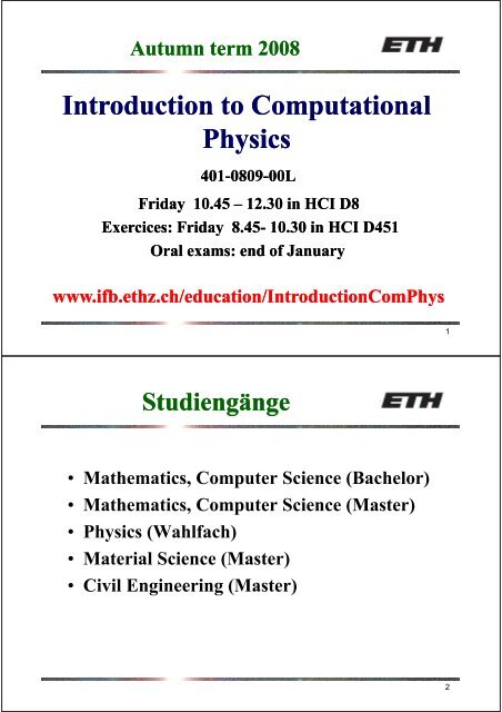
Autumn term 2008<br />
I Introduction t d ti t to C Computational t ti l<br />
Physics<br />
401 401-0809 401 0809-00L 0809 00L<br />
Friday 10.45 – 12.30 in HCI D8<br />
Exercices: Friday 8.45 8.45- 10.30 in HCI D451<br />
Oral exams: end of January<br />
www.ifb.ethz.ch/education/IntroductionComPhys<br />
www www.ifb.ethz.ch/education/IntroductionComPhys<br />
ifb ethz ch/education/IntroductionComPhys<br />
Studiengänge<br />
g g<br />
• Mathematics, Computer Science (Bachelor)<br />
• Mathematics, Computer Science (Master)<br />
• Physics (Wahlfach)<br />
• Material Science (Master)<br />
• Civil Engineering (Master)<br />
1<br />
2
Who is your teacher?<br />
Hans J. J JJ. Herrmann<br />
Herrmann<br />
hjherrmann@ethz.ch<br />
since since April April 2006<br />
2006<br />
<strong>Institute</strong> of <strong>Building</strong> <strong>Materials</strong> (IfB)<br />
HIF E12, Hönggerberg, <strong>ETH</strong> <strong>Zürich</strong><br />
http://comphys.ethz.ch/hans/<br />
Spring term 2008<br />
• Computational Statistical Physics<br />
(H (H.J.Herrmann)<br />
J Herrmann)<br />
• Computational Quantum Physics<br />
(P.Werner, P.de Forcrand, M.Troyer)<br />
• Computational Polymer Physics<br />
(M (M.Kröger) K ö )<br />
3<br />
4
Plan of this course<br />
• 19.09. Introduction, i random numbers (RN)<br />
• 26.09. RN, , Percolation<br />
• 03.10. Fractals, Cellular Automata<br />
• 10 10.10. 10 Random Walks (Kröger)<br />
• 17.10. Finite Size Effects, Monte Carlo<br />
• 24.10. Importance Sampling, Metropolis<br />
• 31 31.10. 10 Ising Model (Werner)<br />
• 07.11. XY Model, first order transitions<br />
Plan of this course<br />
• 14.11. Differential Eqs. (Euler, Runge Kutta..)<br />
• 21.11. Eqs. of Motion (Newton, Regula Falsi)<br />
• 28.11. Finite Difference Meth. Relaxation<br />
• 05.12. Gradient Methods<br />
• 12 12.12. 12 Multigrid Multigrid, Finite Elements Method<br />
• 19.12. Variational FEM, Crank-Nicholson<br />
. Wave equation, Navier-Stokes<br />
5<br />
6
Segregation under vibration<br />
Mixing in a cylinder<br />
Brazil<br />
Nut<br />
Effect<br />
hard<br />
spheres<br />
7<br />
8
Sedimentation<br />
Sedimentation<br />
comparing experiment and simulation<br />
Motion of dunes<br />
V. SCHWÄMMLE, H.J. HERRMANN, Nature 426, 619-620 (2003)<br />
Glass beads<br />
ddescending di<br />
in silicon oil<br />
9<br />
10
Prerequisites<br />
• Ability to work with UNIX<br />
• Making of Graphical Plots<br />
• Higher computer language (FORTRAN, C++..)<br />
• Statistical Analysis (Averaging, Distributions)<br />
• Linear Algebra Algebra, Analysis<br />
• Classical Mechanics<br />
• Basic Thermodynamics<br />
Literature<br />
• H.Gould, J. Tobochnik and W. Christian: „Introduction to<br />
Computer Simulation Methods“ 3rd ed. (Wesley, 2006)<br />
• DD. Landau and K. K Binder: „A A Guide to Monte Carlo<br />
Simulations in Statistical Physics“ (Cambridge, 2000)<br />
• D. Stauffer, , F.W. Hehl, , V. Winkelmann and J.G. Zabolitzky: y<br />
„Computer Simulation and Computer Algebra“ 3rd ed.<br />
(Springer, 1993)<br />
• KBid K. Binder and dDWH D.W. Heermann: „Monte M Carlo C l Simulation Si l i in i<br />
Statistical Physics“ 4th ed. (Springer, 2002)<br />
• NN.J. J Giordano: „Computational Computational Physics Physics“ (Wesley (Wesley, 1996)<br />
• J.M. Thijssen: „Computational Physics“ (Cambridge, 1999)<br />
11<br />
12
Book Series<br />
• „Monte Carlo Method in Condensed Matter<br />
Physics“, ed. K. Binder (Springer Series)<br />
• „Annual Reviews of Computational Physics“, ed.<br />
D. Stauffer (World Scientific)<br />
• „Granada Lectures in Computational Physics“,<br />
ed. J.Marro (Springer Series)<br />
• „Computer Simulations Studies in Condensed<br />
Matter Physics“ Physics , ed ed. D. D Landau (Springer Series)<br />
Journals<br />
• Journal of Computational Physics (Elsevier)<br />
• Computer Physics Communications<br />
(Elsevier)<br />
• IInternational i lJ Journal lof fM Modern d Physics Ph i C<br />
(World Scientific)<br />
every every year year (2007: (2007: Bruxelles, 2008: 2008: Brazil, Brazil, 2009 2009 Taiwan):<br />
Taiwan):<br />
CCP = Conference on Computational Physics<br />
13<br />
14
What is Computational Physics?<br />
• Numerical solution of equations (since<br />
analytical solutions are rare)<br />
• Simulation of many-particle systems (creation<br />
of a virtual reality = 3rd branch of physics)<br />
• Evaluation and visualization of large data<br />
sets (either experimental or numerical)<br />
• Control of experiments p (not ( treated in this course) )<br />
Areas of computational physics<br />
• CFD (Computational Fluid Dynamics)<br />
• Classical Phase Transitions<br />
• Solid State (quantum)<br />
• High Energy Physics (Lattice QCD)<br />
• Astrophysics<br />
• Geophysics, Solid Mechanics<br />
• Agent models (interdisciplinary)<br />
15<br />
16
Computer tools<br />
• Object oriented programming<br />
• Vector supercomputers<br />
• Parallel computing (shared and distributed<br />
memory) )<br />
• Symbolic Algebra (Mathematica, Maple)<br />
• Graphical animations<br />
Why do we need Random numbers?<br />
• Simulate experimental fluctuations (e.g.<br />
radioactive decay)<br />
• Define temperature<br />
• Complement lack of detailed knowledge ( (e.g.<br />
traffic or stock market simulations)<br />
• CConsider id many ddegrees of fffreedom d (e.g.<br />
Bownian motion)<br />
• Test stability to perturbations<br />
• Random sampling<br />
17<br />
18
Literature to Random numbers<br />
• Numerical Recipes<br />
• D.E.Knuth: „ The Art of Programming:<br />
Seminumerical Se u e c Algorithms“ go s 3rd 3 d ed. ed ( (Addison dd so<br />
– Wesley, 1997) Vol. 2, Chapt. 3.3.1<br />
• JE J.E. Gentle, G tl „Random R d Number N b GGeneration ti and d<br />
Monte Carlo Methods“ (Springer, 2003)<br />
Properties p of Random numbers<br />
• No correlations<br />
• Long periods<br />
• Follow well-defined distribution<br />
• Fast implementation<br />
• RReproductibility d tibilit<br />
19<br />
20
Distribution of random numbers<br />
+∞<br />
∫<br />
−∞∞<br />
P( x) dx = 1 and P( x)<br />
> 0<br />
examples: homogeneous, Gaussian, Poisson<br />
Probability to find a random number<br />
i in the h i interval l[ [ [x, , x+ x+Δx]: Δ ] ]:<br />
x +Δ x<br />
wx ( ) = ∫ Pxdx ( )<br />
Random number generators (RNG)<br />
electrical flicker noise<br />
Algorithms:<br />
∫<br />
x<br />
photon emission<br />
f from a semiconductor i d<br />
• Congruential (Lehmer (Lehmer, 1948)<br />
• Lagged-Fibonacci gg (Tausworth,1965)<br />
( , )<br />
21<br />
22
Congruential g generators g<br />
Fix two integers: g c and p.<br />
Start with a seed x0. Create new integers by iterating:<br />
x = ( c⋅x ) p , x , c, p∈Z<br />
i i− i<br />
1 mod<br />
Make random numbers<br />
through<br />
z =<br />
i<br />
x<br />
i<br />
p<br />
Maximal period<br />
z ∈<br />
i<br />
[ 01 , )<br />
Since all all integers integers are are less less than than p the the sequence<br />
sequence<br />
must repeat after at least p-1 1 iterations, i.e.<br />
the maximal period is p-1. 1.<br />
(x (x0 = = 0 0 is is a a fixed fixed point and cannot cannot be used used.) )<br />
R.D. Carmichael proved 1910 that one gets the<br />
maximal period if p is a Mersenne prime number<br />
and and the smallest smallest integer number <strong>for</strong> which<br />
p−1<br />
c mod p<br />
= 1<br />
23<br />
24
Mersenne prime p numbers<br />
n<br />
M = 2 −1<br />
n<br />
43 * December 15,<br />
30,402,457 315416475…652943871 9,152,052<br />
2005<br />
44 * September 4,<br />
32,582,657 124575026…053967871 9,808,358<br />
2006<br />
Example p of congruential g RNG<br />
Park and Miller (1988):<br />
const int p=2147483647;<br />
const int c=16807;<br />
int int rnd=42; rnd=42; //seed<br />
rnd = (c*rnd) % p;<br />
print rnd;<br />
GIMPS / Curtis<br />
& Steven Boone<br />
GIMPS / Curtis<br />
& Steven Boone<br />
25<br />
26
Applet<br />
x i+1<br />
Square test<br />
Theorem of Marsaglia g<br />
x<br />
(1968)<br />
For a congruential generator the random<br />
numbers b i in an n-cube cube-test b t ttest t li lie on parallel ll l<br />
n-1 n 1 1 dimensional dimensional hyperplanes.<br />
∃ a a a x + a x + + a x p =<br />
1 1,..., , , n : ( 1 i 2 i + 1 ... n i + n n− 1 ) mod p 0<br />
proof using:<br />
∃∀ pcn , , at least one set<br />
a a,..., a :<br />
( 1<br />
n )<br />
1 ... ) n<br />
ac + + a c mod p =<br />
1 n p<br />
1<br />
0<br />
n<br />
27<br />
28
n-cube cube-test test<br />
One One can can also sho show that that <strong>for</strong> <strong>for</strong> congruential congr ential RNG<br />
RNG<br />
the distance between the planes p must be larger g<br />
than<br />
p<br />
n<br />
and that the maximum number of planes is<br />
p<br />
1 n<br />
Lagged Lagged-Fibonacci Fibonacci RNG<br />
• Initialization ii i i of fbb random bits i xi • AApply: l<br />
(∑ ( ∑ j∈ℑ<br />
x = x ) mod 2<br />
i<br />
i i−<br />
j<br />
ℑ<br />
⊂<br />
[ 1,..,<br />
,,<br />
b ]<br />
29<br />
30
Lagged gg Fibbonacci RNG<br />
Typically one uses, since it is easy to implement:<br />
x = x ⊕x ≡ x + x<br />
( ) mod 2<br />
i i−a i−b i−a i−b a < b<br />
Theorem of fA A. C Compagner (1992):<br />
If If ( (a,b ( (a,b a,b) ) Zierler trinomial then then sequence sequence has<br />
has<br />
maximal period 2 2b – 1 and :<br />
2<br />
x ⋅x − x = 0 ∀ k < b<br />
i i−k i<br />
Zierler trinomials<br />
1+ x<br />
a<br />
+ x<br />
b<br />
primitive on Z Z2[x] (Zierler, 1969)<br />
(a, ( , b) )<br />
(103, 250) (Kirkpatrick and Stoll, 1981)<br />
(1689, 4187)<br />
(54454, 132049) (J.R. Heringa et al, 1992)<br />
(3037958 (3037958, 6972592) (R.P.Brent et al., 2003)<br />
31<br />
32
Making 64 64-bit bit integers<br />
..…<br />
z zi = (01101….101110)<br />
(01101 101110)<br />
z i+1 +1 = (10001….010111)<br />
zi+2 i+2 2 = (00101….111001)<br />
( )<br />
zi+3 +3 = (01011….011100)<br />
zi+4 +4 = (00011….011011)<br />
.....<br />
Tests <strong>for</strong> random numbers<br />
• Check distribution<br />
• Average is 0.5<br />
• Average of each bit is 0.5<br />
• n-cube-test n cube test<br />
• Correlations should vanish<br />
• SSpectral t lt test: t no peaks k iin Fourier F i trans<strong>for</strong>m t f<br />
• χ2 χ test: partial p sums follow a Gaussian<br />
• Kolmogorov – Smirnov test<br />
→ „Diehard Di h d battery“ b tt “ of f M Marsaglia li (1995)<br />
33<br />
34
Diehard battery<br />
• Birthday Spacings: Choose random points on a large interval. The spacings between the points should be Poisson<br />
distributed.<br />
• Overlapping Permutations: Analyze sequences of five consecutive random numbers numbers. The 120 possible orderings<br />
should occur with statistically equal probability.<br />
• Ranks of matrices: Select some number of bits from some number of random numbers to <strong>for</strong>m a matrix over<br />
{0,1}, then determine the rank of the matrix. Count the ranks.<br />
• Monkey Tests: Tests: Treat sequences of some number of bits as "words" words . Count the overlapping words in a stream stream.<br />
The number of "words" that don't appear should follow a known distribution.<br />
• Count the 1s: Count the 1 bits in each of either successive or chosen bytes. Convert the counts to "letters", and<br />
count the occurrences of five-letter "words".<br />
• Parking Lot Test: Randomly place unit circles in a 100 x 100 square square. If the circle overlaps an existing one one, try<br />
again. After 12,000 tries, the number of successfully "parked" circles should follow a normal distribution.<br />
• Minimum Distance Test: Randomly place 8,000 points in a 10,000 x 10,000 square, then find the minimum<br />
distance between the pairs. The square of this distance should be exponentially distributed.<br />
• Random Spheres Test: Randomly choose 44,000 000 points in a cube of edge 11,000. 000 Center a sphere on each point, point<br />
whose radius is the minimum distance to another point. The smallest sphere's volume should be exponentially<br />
distributed with a certain mean.<br />
• The Squeeze Test: Multiply 231 by random floats on [0,1) until you reach 1. Repeat this 100,000 times. The<br />
number u be oof floats oats needed eeded to reach eac 1 should s ou d follow o ow a certain ce ta distribution.<br />
d st but o .<br />
• Overlapping Sums Test: Generate a long sequence of random floats on [0,1). Add sequences of 100 consecutive<br />
floats. The sums should be normally distributed with characteristic mean and sigma.<br />
• Runs Test: Generate a long sequence of random floats on [0,1). Count ascending and descending runs. The counts<br />
should follow a certain distribution.<br />
• The Craps Test: Play 200,000 games of craps, counting the wins and the number of throws per game and check<br />
the distribution.<br />
RN with other distributions<br />
• Trans<strong>for</strong>mation method<br />
Poisson distribution<br />
Gaussian distribution<br />
(Box (B (Box Muller, M ll 1958)<br />
1958)<br />
• Rejection method<br />
35<br />
36
Trans<strong>for</strong>mation method<br />
We want random numbers y distributed as P(y). (y) ).<br />
Start with homogeneously g y ⎧1 if z ∈ [ 0 , 1 ]<br />
distributed numbers z:<br />
P(y)<br />
y z<br />
⎪<br />
P ( z ) = ⎨<br />
⎪⎩<br />
Trans<strong>for</strong>mation method<br />
example:<br />
p<br />
generate Poisson distribution:<br />
y<br />
'<br />
y y<br />
−<br />
' k y<br />
ke k dy [ e ] 0 1<br />
y<br />
−<br />
k<br />
−<br />
∫ =−<br />
0<br />
z = = −e<br />
( 1 )<br />
⇒ y =−kln −z<br />
z<br />
0 otherwise<br />
y<br />
' ' ' '<br />
∫ ∫<br />
z = P( z ) dz = P( y ) dy<br />
0 0<br />
y<br />
P( y) ke k<br />
−<br />
=<br />
where z ∈ [0,1) are homogeneous random numbers.<br />
This method only works if the integral can be<br />
solved l d and dth the resulting lti function f ti can be b inverted.<br />
i t d<br />
37<br />
38
Box –Muller Muller (1958)<br />
Gaussian distribution:<br />
distribution:<br />
y y2<br />
1 −<br />
e dy σ<br />
z e σ dy<br />
∫<br />
0<br />
πσ<br />
P( y) 1 −<br />
y<br />
e σ =<br />
πσ<br />
= ∫ cannot be solved in closed <strong>for</strong>m.<br />
trick:<br />
r = y + y<br />
y<br />
tan tanϕϕ<br />
=<br />
y<br />
2 2 2<br />
1 2<br />
1 2<br />
1<br />
2<br />
dyy dyy = rdrdϕϕ<br />
y 2 y 2<br />
y y 1 1 y y<br />
2<br />
2<br />
1 −<br />
σ 1 −<br />
σ<br />
e e<br />
∫ ∫<br />
z ⋅ z = dy ⋅<br />
dy<br />
1 2 1 2<br />
0 πσ 0 πσ<br />
y y y2 2 2<br />
1 + y2 ϕ r r<br />
− −<br />
σ σ<br />
1 2<br />
1 1<br />
∫∫ ∫∫<br />
e e<br />
= dy dy = rdrdϕ<br />
πσ πσ<br />
1 2<br />
0 0 0 0<br />
2<br />
ϕ σ<br />
1 ⎛ y ⎞<br />
= = ⎜ ⎟<br />
πσ 2 2 2ππ ⎝ y2<br />
⎠<br />
Box –Muller Muller trick<br />
1 ⎛ y ⎞ 1<br />
z1⋅ z2<br />
= ⎜ ⎟⋅<br />
2π<br />
⎝ y2<br />
⎠<br />
( 1 )<br />
y + y =−σln −z<br />
2 2<br />
1 2 2<br />
y sin 2π<br />
z<br />
= tan 2π<br />
z =<br />
y z<br />
1 1<br />
2<br />
1<br />
cos 2 2π<br />
1<br />
1<br />
( 1−e σ ) arctan ( 1−e<br />
σ )<br />
2<br />
2 2<br />
1 + 2<br />
r<br />
y y<br />
− −<br />
2 2<br />
1+ 2<br />
y y<br />
−<br />
e σ<br />
arctan ( 1−<br />
)<br />
⇒<br />
( )<br />
y = −σσ ln 1 1− z sin 2 2ππ<br />
z<br />
1 2 1<br />
= − ( −<br />
π ( )<br />
y σ ln 1 z cos 2πz<br />
2 2 1<br />
From two homogeneously g y distributed random<br />
numbers z1 and z 2 one gets two Gaussian<br />
distributed random numbers y1 and y2 .<br />
39<br />
40
Rejection method<br />
Generate random numbers y ∈ [0, [, [0,B] ] sampled p<br />
according to a distribution P(y) ) with P(y) < AA.<br />
.<br />
Sample two homogeneously<br />
distributed random numbers<br />
z 1 ,<br />
, z 2 ∈ [0,1)<br />
[0,1). . If the point<br />
(B (Bz Bz1, , A Az Az2) )li ) lies above b the th curve<br />
P(y), ), i.e. P(Bz Bz1) < Az Az2 then<br />
reject the attempt, otherwise y = Bz Bz1 is retained as a<br />
random number which which is is distributed according to P(y). ).<br />
P<br />
41