Proceso de diseño

INTRODUCCION AL PROYECTO DE INGENIERIA: Optimización
∂ E
∂ x 1
+
∂ h
λ .
∂ x 1
= 0
y repitiendo el proceso para la expresión (24), se obtiene también
∂ E
∂ x 2
∂ h
+ λ .
∂ x 2
= 0
Todo esto puede ponerse de un modo simplificado en la forma
∂
∂x
∂
∂ x
1
2
( E + λ . h ( x , x ) ) = = 0
1
2
∂L
∂x
1
∂ L
∂ x
( E + λ . h ( x , x ) ) = = 0
1
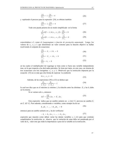
conociéndose a L como el Langrangiano o función de prestación aumentada. Luego, los
valores de x1, x2 y λ que determinan un valor extremo para la función objetivo se hallan
resolviendo el conjunto de ecuaciones
∂ L
∂ x
1
∂ L
∂ x
2
=
=
E
∂ L
= h
∂ λ
E
3
1
2
+ λ h
=
0
1
+ λ h
2
=
=
2
0
en las cuales el multiplicador de Lagrange se trata como si fuera una variable independiente
mas, en lo que respecta a las derivadas parciales. Se tiene por tanto, en este caso, un sistema de
tres ecuaciones con tres incógnitas: x1, x2 y λ. Obsérvese que la restricción impuesta por la
ecuación (32) no es más que otra forma de expresar la condición
h ( x 1 , x 2 ) = 0
(33)
Además, de las expresiones (30) a (32) se deduce que
E 1 E 2
+ = λ
(34)
( − h1
) ( − h 2 )
la cual nos dice que en el máximo (o mínimo ), la relación entre las distintas Ei y las hi debe
ser la misma.
Si se variara solo xi, entonces
∆ E =
∂E
. ∆x
i
∂x
i
= E i . ∆x
i
(35)
Esta expresión indica que un cambio unitario en xi (∆xi=1) provoca un cambio Ei
en E, ∆E=Ei. Pero además, considerando n variables, como siempre ha de ser
h dx ..... + h = 0
(36)
1 . 1 + n dx n
entonces para un cambio unitario en xi, ha de verificarse
− h i = h . ∆ x + ..... + h n . ∆ x
(37)
2 2
n
expresión que muestra como deben variar las demás variables xj ( j≠i) para que continúe
cumpliéndose la restricción; se observa que la variación de estas debe ser ponderada por el
valor de hi, valor este que mide la importancia o peso de la variable en la restricción.
0
2
(26)
(27)
(28)
(29)
(30)
(31)
(32)
67
67