Optimización Estocástica de Planes de Desarrollo - MEIVAP

Producción Promedio Dia Ano 2 Producción Ano 2 - Anualizada
Ingresos Esperados Ano 2
Precio del Hidrocarburo
Precio del Crudo ($/bl)
X 365 días =
X
=
70.00 76.75 83.50 90.25 97.00
Producción Promedio Dia Global (MMPCGD)
100
90
80
70
60
50
40
30
20
10
0
Año
Producción
(bpd)
Producción
Vendida
Anualizada
(bpd)
Ingresos antes de
Impuestos
($/año)
0 0.00 0.00
1 504.47 184131.61 11661668.89
2 421.37 153799.65 9740644.64
3 351.96 128464.27 8136070.31
4 293.98 107302.38 6795817.17
5 245.55 89626.48 5676343.64
6 205.10 74862.33 4741280.75
7 171.32 62530.27 3960250.58
8 143.09 52229.67 3307879.34
9 119.52 43625.89 2762973.07
10 99.83 36439.41 2307829.10
2
Pronóstico de Producción de Gas - Campo R2M
Qdia10% QdiaMEDIA Qdia90% Gp10% GpMEDIA Gp90%
250,000
200,000
150,000
100,000
50,000
0
Producción Acumulada Global (MMPCG)
Ingresos (MM$)
25
20
15
10
5
0
Perfil de Ingresos (MM$)
1 2 3 4 5 6 7 8 9 10
Tiempo (años)
P10 P50 P90
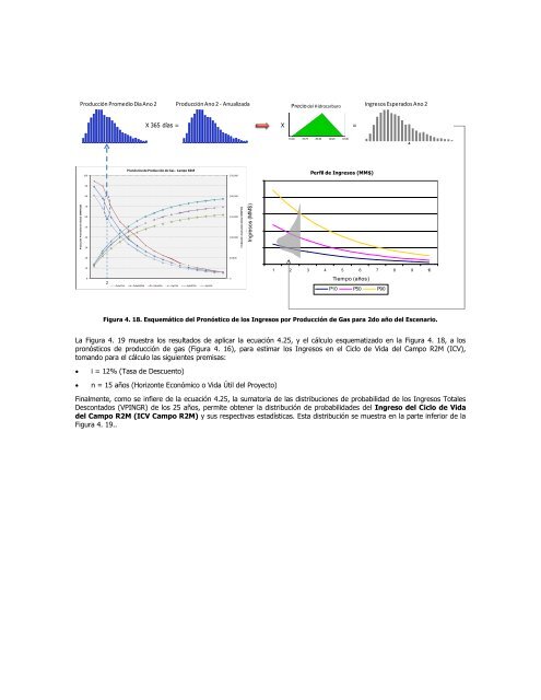
Figura 4. 18. Esquemático del Pronóstico de los Ingresos por Producción de Gas para 2do año del Escenario.
La Figura 4. 19 muestra los resultados de aplicar la ecuación 4.25, y el cálculo esquematizado en la Figura 4. 18, a los
pronósticos de producción de gas (Figura 4. 16), para estimar los Ingresos en el Ciclo de Vida del Campo R2M (ICV),
tomando para el cálculo las siguientes premisas:
i = 12% (Tasa de Descuento)
n = 15 años (Horizonte Económico o Vida Útil del Proyecto)
Finalmente, como se infiere de la ecuación 4.25, la sumatoria de las distribuciones de probabilidad de los Ingresos Totales
Descontados (VPINGR) de los 25 años, permite obtener la distribución de probabilidades del Ingreso del Ciclo de Vida
del Campo R2M (ICV Campo R2M) y sus respectivas estadísticas. Esta distribución se muestra en la parte inferior de la
Figura 4. 19..