variabilité interannuelle et tendances. Comparaison aux ... - LMD

42
CHAPITRE 3. L’EAU CONTINENTALE VUE PAR L’ALTIMÉTRIE SPATIALE ET
PAR ORCHIDEE
80°N
80°N
40°N
40°N
0°
0°
40°S
40°S
80°S
80°S
100°W
0° 100°E
100°W 0° 100°E
0 1
(a) AMIP simulation
2 4 6 8 10 12
(b) CRU observations
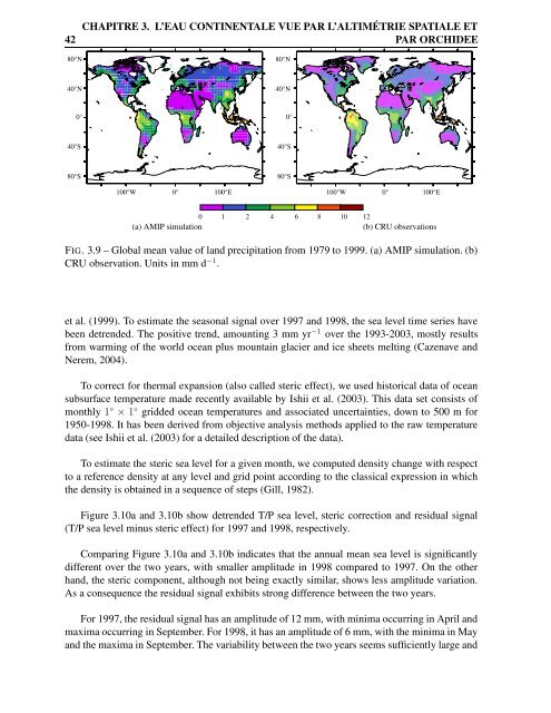
FIG. 3.9 – Global mean value of land precipitation from 1979 to 1999. (a) AMIP simulation. (b)
CRU observation. Units in mm d −1 .
et al. (1999). To estimate the seasonal signal over 1997 and 1998, the sea level time series have
been detrended. The positive trend, amounting 3 mm yr −1 over the 1993-2003, mostly results
from warming of the world ocean plus mountain glacier and ice sheets melting (Cazenave and
Nerem, 2004).
To correct for thermal expansion (also called steric effect), we used historical data of ocean
subsurface temperature made recently available by Ishii et al. (2003). This data set consists of
monthly 1 ◦ × 1 ◦ gridded ocean temperatures and associated uncertainties, down to 500 m for
1950-1998. It has been derived from objective analysis methods applied to the raw temperature
data (see Ishii et al. (2003) for a detailed description of the data).
To estimate the steric sea level for a given month, we computed density change with respect
to a reference density at any level and grid point according to the classical expression in which
the density is obtained in a sequence of steps (Gill, 1982).
Figure 3.10a and 3.10b show detrended T/P sea level, steric correction and residual signal
(T/P sea level minus steric effect) for 1997 and 1998, respectively.
Comparing Figure 3.10a and 3.10b indicates that the annual mean sea level is significantly
different over the two years, with smaller amplitude in 1998 compared to 1997. On the other
hand, the steric component, although not being exactly similar, shows less amplitude variation.
As a consequence the residual signal exhibits strong difference between the two years.
For 1997, the residual signal has an amplitude of 12 mm, with minima occurring in April and
maxima occurring in September. For 1998, it has an amplitude of 6 mm, with the minima in May
and the maxima in September. The variability between the two years seems sufficiently large and