Materiali e Tecnologie per la realizzazione di sostituti - FedOA ...

UNIVERSITÀ DEGLI STUDI DI NAPOLI “FEDERICO II”
FACOLTÀ DI INGEGNERIA
DIPARTIMENTO DI INGEGNERIA DEI MATERIALI
E DELLA PRODUZIONE
DOTTORATO DI RICERCA IN INGEGNERIA CHIMICA
DEI MATERIALI E DELLA PRODUZIONE
XVIII° CICLO
MATERIALI E TECNOLOGIE PER LA
REALIZZAZIONE DI SOSTITUTI OSSEI
NELL’INGEGNERIA DEI TESSUTI
Coordinatore: Candidato:
CH. MO PROF. N.GRIZZUTI ING. VINCENZO GUARINO
Tutor:
CH. MO PROF. L. AMBROSIO
CH. MO PROF. P.A. NETTI
TRIENNIO ACCADEMICO 2002/2005

INDICE
INDICE .................................................................................................................. 3
INTRODUZIONE................................................................................................. 7
1. L’OSSO NATURALE ........................................................................................13
1.1 PREMESSE......................................................................................................................... 13
1.2 ASPETTI GENERALI ..................................................................................................... 13
1.3 IL RIMODELLAMENTO OSSEO ............................................................................... 14
1.4 RELAZIONI TRA STRUTTURA E PROPRIETA’................................................... 17
1.5 STATI DI SOLLECITAZIONE DELL’OSSO............................................................ 24
2. INGEGNERIA DEI TESSUTI........................................................................ 28
2.1 DEFINIZIONE .................................................................................................................28
2.2 TAPPE EVOLUTIVE....................................................................................................... 29
2.2 TISSUE REGENERATION ........................................................................................... 32
2.3 LE CELLULE..................................................................................................................... 33
2.4 COLTURE IN VITRO: BIOREATTORI.................................................................... 34
3. SCAFFOLDS TRIDIMENSIONALI............................................................... 39
3.1 DEFINIZIONE .................................................................................................................39
3.2 PROGETTAZIONE DI SCAFFOLDS ....................................................................... 39
3.3 MATERIALI IMPIEGATI .............................................................................................. 41
3.4 REQUISITI STRUTTURALI: POROSITA’................................................................. 45
3.5 TECNICHE DI PREPARAZIONE .............................................................................. 48
4. MATERIALI, METODI E STRUMENTAZIONE........................................ 57
4.1 MATERIALI IMPIEGATI .............................................................................................. 57
4.1.1 Il POLICAPROLATTONE (PCL).......................................................................... 57
4.1.2 DERIVATI DELL’ACIDO IALURONICO......................................................... 60
a) L’Acido Ialuronico .......................................................................................................... 60
b) Gli HYAFF.................................................................................................................. 61
4.1.3 FOSFATI DI CALCIO: HA, α-TCP ....................................................................... 64
a) Aspetti generali................................................................................................................ 64
b) Aspetti termodinamici...................................................................................................... 67
c) Reazione di hardening - Chimica della reazione ............................................................... 68
d) Reazione di hardening - Cinetica della reazione ............................................................... 69
e) effetto della temperatura .................................................................................................... 70
f) effetto della porosità........................................................................................................... 71
g) effetto del magnetismo........................................................................................................ 71
4.2 PREPARAZIONE DEL SUBSTRATO ........................................................................ 73
4.2.1 SCAFFOLD MACROPOROSI................................................................................ 73
4.2.2 SCAFFOLD MACROPOROSI FIBRORINFORZATI...................................... 79
4.2.3 SCAFFOLD MACROPOROSI PER SEPARAZIONE DI FASE ................... 84
4.2.4 MICROSFERE E SCAFFOLD SINTERIZZATI................................................ 86
3

4
a) Singola emulsione .............................................................................................................86
b) Doppia emulsione.............................................................................................................87
c) Pseudo-Sinterizzazione delle microsfere..............................................................................89
4.3 TIPOLOGIE DI CAMPIONI .........................................................................................91
4.4 ANALISI DEI CAMPIONI .............................................................................................96
4.4.1 ANALISI MORFOLOGICA ....................................................................................96
Microscopio a scansione elettronica ( SEM )..........................................................................96
4.4.2 CARATTERIZZAZIONE MECCANICA............................................................99
Macchina dinamometrica Instron 4204: Principio di funzionamento......................................99
4.4.3 ANALISI TERMICA................................................................................................101
Calorimetro a scansione differenziale (DSC): principio di funzionamento.............................101
4.4.4 ANALISI POROSIMETRICA ...............................................................................103
a) Analisi qualitativa: metodo gravimetrico e liquid displacement.........................................103
b) Analisi quantitativa: porosimetria ad intrusione di mercurio............................................104
c) Analisi qualitativa: analisi di immagini 2D ...................................................................109
4.4.5 ANALISI SPETTROSCOPICA E.D.S. ................................................................110
4.4.6 COLTURA CELLULARE.......................................................................................111
a) Bio-reattore di semina.....................................................................................................112
b) Test di vitalità cellulare: Alamar Blue reduction .............................................................113
c) Effetto della semina dinamica sulla distribuzione cellulare: analisi al microscopio confocale 114
5. ANALISI SPERIMENTALE...........................................................................117
5.1 SCAFFOLD MACROPOROSI – SALT LEACHING .............................................117
5.1.1 ANALISI MORFOLOGICA E MICROSTRUTTURALE...............................117
5.1.2 ANALISI POROSIMETRICA ...............................................................................124
a) Metodo gravimetrico e liquid displacement .......................................................................124
b) Analisi di immagini 2D ................................................................................................126
c) Porosimetria ad intrusione di mercurio.............................................................................135
5.1.3 ANALISI TERMICA................................................................................................140
5.1.4 CARATTERIZZAZIONE MECCANICA..........................................................142
5.1.5 MODELLO TEORICO E DATI SPERIMENTALI.........................................147
a) Porosità e rapporto Superficie/Volume ...........................................................................147
b) Comportamento meccanico di uno scaffold: compressione e trazione ...................................149
5.1.6 SEMINA CELLULARE: STATICA E DINAMICA ........................................152
5.2 SCAFFOLD MACROPOROSI FIBRORINFORZATI............................................157
5.2.1 ANALISI MORFOLOGICA E MICROSTRUTTURALE...............................157
5.2.2 ANALISI POROSIMETRICA ...............................................................................161
5.2.3 CARATTERIZZAZIONE MECCANICA..........................................................162
5.2.4 VALUTAZIONE DEL RAPPORTO FIBRA/MATRICE...............................164
5.3 SCAFFOLD MACROPOROSI – SEPARAZIONE TIPS .......................................166
5.3.1 ANALISI TERMICA PRELIMINARE ................................................................166
5.3.2 ANALISI MORFOLOGICA E MICROSTRUTTURALE...............................168
5.3.2 ANALISI POROSIMETRICA ...............................................................................173
a) Metodo gravimetrico........................................................................................................173
b) Analisi 2D di immagini ................................................................................................175
c) Porosimetria ad intrusione di mercurio.............................................................................183
5.4 MICROSFERE E PSEUDOSINTERIZZAZIONE .................................................187
5.4.1 SINGOLA EMULSIONE.......................................................................................187
a) Analisi morfologica ........................................................................................................187

) Analisi calorimetrica...................................................................................................... 190
5.4.2 DOPPIA EMULSIONE.......................................................................................... 192
a) Analisi morfologica........................................................................................................ 192
b) Analisi porosimetrica ad intrusione di mercurio............................................................... 195
c) Analisi al microscopio confocale....................................................................................... 197
5.4.3 PSEUDO SINTERIZZAZIONE PER FUSIONE (MIMS) ............................ 198
a) Analisi morfologica........................................................................................................ 199
b) Analisi porosimetrica ad intrusione di mercurio............................................................... 205
c) Caratterizzazione meccanica........................................................................................... 206
6. DISCUSSIONE .............................................................................................. 208
7. SVILUPPI FUTURI ........................................................................................217
7.1 ELETTROSPINNING................................................................................................... 217
7.2 BLENDS COCONTINUE BIODEGRADABILI .................................................... 221
CONCLUSIONI..................................................................................................231
APPENDICI....................................................................................................... 235
I) SEPARAZIONE DI FASE............................................................................. 235
I.a) TECNICHE DI OTTENIMENTO DELLE STRUTTURE POROSE..... 235
I.b) DIAGRAMMI DI FASE DI SISTEMI TERNARI........................................ 236
I.c) ASPETTI TERMODINAMICI.......................................................................... 238
I.d) ASPETTI CINETICI ........................................................................................... 248
I.e) FATTORI DETERMINANTI SULLA STRUTTURA................................. 250
II) DIFFUSIONE ATTRAVERSO MEMBRANE POROSE ...........................251
II.a) TEORIA DEL TRASPORTO DI MATERIA ............................................... 251
II.b) FENOMENI DI TRASPORTO IN MEMBRANE POROSE................... 251
II.c) TRASPORTO DI MATERIA A SEGUITO DI ∆P IMPOSTO ................ 254
II.d) PERFUSIONE: MODELLO DI BOTCHWAY/LAURENCIN............... 255
III) ELABORAZIONE DI IMMAGINI 2D...................................................... 257
RIFERIMENTI BIBLIOGRAFICI:.................................................................. 263
5

INTRODUZIONE
La perdita o l’insufficienza funzionale di un tessuto rappresenta certamente uno
dei problemi più invalidanti, frequenti e costosi nell’ambito della medicina
internazionale [ 1 ].
Infatti, tale problema non si limita solamente ai casi in cui si prospetta la totale
assenza di organi, ma coinvolge anche quei casi in cui la mancanza del tessuto,
pur essendo localizzata in zone circoscritte dell’organismo, determina una
riduzione significativa della qualità della vita del paziente.
L’approccio tradizionale nel recupero delle funzioni fisiologiche di organi e
tessuti danneggiati si fonda sull’utilizzo di protesi artificiali le quali, malgrado i
notevoli progressi compiuti negli ultimi anni circa la definizione di nuovi materiali
e di nuove tecnologie, presentano alcuni limiti intrinseci dai quali, attualmente,
ancora non si può prescindere. Il motivo principale di queste difficoltà nasce dalla
volontà di voler sostituire una parte di un sistema vivente così complesso con un
sistema artificiale inevitabilmente più semplificato. A ciò si aggiungono una
miriade di problematiche connesse alla risposta dell’organismo in presenza di
corpi estranei, di fatto, ancora non completamente risolvibili.
I progressi raggiunti nella ricerca di materiali innovativi negli ultimi anni
permettono la realizzazione di nuovi sistemi protesici in grado di presentare
risultati apprezzabili in termini di qualità della vita del paziente anche lungo un
arco temporale relativamente breve [ 2 ].
Una diversa soluzione al problema della degenerazione dei tessuti risulta essere
l’impiego del trapianto di organi naturali. Esso, se da un lato permette di
recuperare integralmente le funzionalità dell'organo da sostituire presenta ancora
due problemi di estrema rilevanza: in primo luogo il rigetto, ovvero una risposta
immunitaria negativa dell'organismo nei confronti dell'organo trapiantato, a cui si
affianca, con crescente allarme, la sempre più scarsa disponibilità di organi da
impiantare. Basti pensare che, nel 1996 negli Stati Uniti, su 50.000 pazienti in
attesa di trapianto di cuore solo 7.500 sono riusciti ad ottenerlo (circa il 15% del
totale) ed il dato è in continua crescita [ 1 ].
Da un lato la richiesta crescente di organi artificiali e di supporti protesici dovuta
principalmente all’incremento dell’età media degli individui ed ad una loro
maggiore disponibilità economica, dall’altro i progressi raggiunti sia nelle
metodologie di coltura cellulare che nella ricerca di nuovi biomateriali, hanno
alimentato la possibilità di riparare i tessuti danneggiati attraverso la crescita
localizzata di nuovo tessuto laddove si verifica la degenerazione in modo da
ripristinare il tessuto originale [ 2 ].
7

8
In altri termini la soluzione innovativa al problema della degenerazione tessutale
risiede nella moderna ingegneria dei tessuti la quale, attingendo da un lato dalla
biologia e dalla medicina per quanto concerne le relazioni struttura-funzione dei
tessuti naturali e dall’altro dall’ingegneria chimica, dei materiali e dalla
bioingegneria in merito allo sviluppo di biomateriali innovativi, consente la
progettazione di strutture tridimensionali (scaffolds) in cui le cellule viventi,
introdotte mediante mirate procedure di coltura in vitro, sono in grado di
differenziare, proliferare ed organizzarsi come nel tessuto nativo in modo da
riprodurre fedelmente l’elemento naturale danneggiato da sostituire.
I biomateriali utilizzati nella rigenerazione tissutale sono molteplici e si possono
distinguere in base alla loro natura chimica (ceramici, polimeri, compositi) nonché
alle intrinseche proprietà fisiche e microstrutturali (biodegradabili o permanenti;
naturali, sintetici o ibridi; permeabili, semipermeabili o non permeabili).
In ogni caso, essi devono mostrare un’elevata biocompatibilità intesa come la
capacità del materiale di indurre una risposta biologica in grado di favorire il
recupero funzionale del tessuto nella sede dell’impianto senza interferire con i
meccanismi di rigenerazione tessutale o produrre reazioni infiammatorie o
immunitarie avverse (citotossicità).
Inoltre la compatibilità biologica costituisce una condizione necessaria ma non
sufficiente affinché un impianto non produca alterazioni nel tessuto ospite.
Come sottolineato dagli studiosi Wintermantel e Mayer non è possibile prescindere
dalla compatibilità strutturale intesa come la capacità del materiale di adattarsi in
maniera ottimale al tessuto ospite da un punto di vista meccanico ottimizzando la
trasmissione dei carichi e minimizzando la deformazione dell’interfaccia
tessuto/impianto [ 3 ].
Il policaprolattone (PCL), preso in esame in questo lavoro di tesi, risulta in questa
direzione uno dei biomateriali di nuova concezione di maggiore diffusione nel
settore dell’ingegneria tessutale. Usato inizialmente per la realizzazione di film
degradabili e stampi, oggi, esso trova largo impiego in vari settori delle
biotecnologie quali l’organ substitution nella realizzazione di suture riassorbibili, il
drug delivery per sistemi a rilascio controllato di farmaci nonché, negli ultimi anni,
nella tissue regeneration per la realizzazione di strutture temporanee (scaffolds)
sostitutive del tessuto osseo naturale.
Un così ampio e diversificato insieme di impieghi è legittimato da caratteristiche
chimiche e fisiche del polimero del tutto particolari soprattutto in relazione alla
cinetica dei meccanismi di degradazione nonché ad acclarate doti di
biocompatibilità ampiamente documentate in letteratura indispensabili per la
riuscita della generica applicazione in campo biomedicale [ 4 ].

In questa sede si propone l’utilizzo del PCL per la realizzazione di scaffolds
tridimensionali ottenuti mediante diverse metodologie e tecniche di realizzazione
al fine di sostituire, in termini meccanici e microstrutturali, tessuti duri
mineralizzati ed in particolare il tessuto osseo trabecolare.
L’obiettivo principale di questo studio è rivolto al raggiungimento di una porosità
opportuna all’interno della struttura polimerica caratterizzata da un elevato grado
di interconnessione dei pori ed una distribuzione spaziale omogenea in grado di
favorire i meccanismi di adesione, differenziamento e proliferazione cellulare e di
fornire lo spazio necessario per la neovascolarizzazione dei tessuti circostanti in
vivo consentendo sia la circolazione di sostanze nutritive indispensabili al
sostentamento cellulare che l’eliminazione di scorie e sostanze metaboliche di
rifiuto.
Al contempo i tempi di degradazione del polimero, opportunamente lunghi,
consentono alla struttura polimerica di mantenere gli spazi necessari all’interno
dello scaffold affinché le cellule possano proliferare fino alla completa ricrescita
del tessuto in formazione [ 5 ]. Inoltre non bisogna dimenticare che esiste un
intimo legame, ancora non completamente spiegato in letteratura, tra la natura
dell’architettura dei tessuti ed il microambiente ideale alla loro rigenerazione.
In altri termini per ogni tipologia di tessuto esiste una dimensione ottimale dei
pori all’interno dello scaffold che consente alle cellule di attivarsi in modo da
riprodurne la struttura. In quest'ottica, nel caso della rigenerazione del tessuto
osseo, molti ricercatori indicano un range dimensionale ottimale dei pori
compreso tra 150 e 400 µm [ 6 ][ 7 ], anche se altri studiosi (Yoshikawa ed altri)
ritengono preferibili pori di dimensioni più elevate (400-500 µm) [ 8 ].
In questo lavoro di tesi si propone la realizzazione di scaffold macroporosi in
policaprolattone mediante le seguenti tecniche:
1. Phase inversion/particulate leaching (PI/SL)
2. Separazione di fase indotta dalla temperatura (TIPS);
3. Pseudo-sinterizzazione per fusione di microsfere (MIMS);
La tecnica del phase inversion/salt leaching consente di realizzare scaffold a
porosità controllata mediante l’impiego di agenti porogeni, generalmente cristalli
di NaCl e/o saccarosio. La loro estrazione dal network polimerico permette di
ottenere strutture macroporose (L-macropori) con grado di porosità superiore al
90% in volume ed elevato grado interconnessione dei pori. Attraverso un’attenta
selezione della forma e delle dimensioni dei cristalli è possibile modulare la forma
e la dimensione media dei pori all’interno del costrutto.
In aggiunta, la separazione termodinamica polimero/solvente indotta da un
opportuno non solvente consente di realizzare una macroporosità di scala ridotta
9

10
(S-macropori) in grado di favorire il trasporto delle sostanze nutritive e la
rimozione delle sostanze di rifiuto nonché la vascolarizzazione del tessuto di
neoformazione.
In questo lavoro di tesi si propone la realizzazione di scaffold polimerici e
compositi a base di policaprolattone (PCL) mediante la tecnica suddetta in
relazione alle specifiche esigenze dettate dall’applicazione di interesse.
Su di essi è stata effettuata una caratterizzazione morfologica e strutturale
attraverso microscopia a scansione elettronica (S.E.M.) supportata da misure di
porosità (metodo gravimetrico, analisi di immagini 2D, porosimetria ad
intrusione di mercurio) finalizzate a qualificare ed a quantificare la porosità dello
scaffold (grado di porosità percentuale, grado di interconnessione dei pori,
diametro medio, rapporto superfice/volume).
Nei casi di maggiore interesse, è stata effettuata una caratterizzazione meccanica
(trazione e/o compressione) al fine di valutare la compatibilità con la risposta
meccanica dell’osso spongioso. In questa direzione, la matrice polimerica di PCL
è stata affiancata da segnali bioattivi di diversa natura: a) idrossiapatite al fine di
migliorare le proprietà di osteoinduzione migliorando la capacità di
osteointegrazione con i tessuti circostanti; b) fosfato tricalcico al fine di
migliorare le proprietà osteoinduttive innescando la formazione di nuovo tessuto
osseo; c) estere benzilico dell’acido ialuronico (HYAFF11) al fine di migliorare
ulteriormente la compatibilità della struttura favorendo i meccanismi di adesione,
proliferazione e differenziamento cellulare [ 9 ].
In alternativa, la matrice polimerica in PCL è stata affiancata da sistemi di
rinforzo fibroso (acido polilattico) e/o particellare (fosfato tricalcico α-TCP)
in grado di migliorare la risposta meccanica complessiva del supporto in modo da
favorirne la mimesi con il tessuto osseo trabecolare che si propone di sostituire.
Le tecniche di separazione di fase indotta dalla temperatura (TIPS) consente la
realizzazione di strutture macroporose in virtù della transizione termodinamica
solido/liquido di un sistema polimero/solvente.
Attraverso un’adeguata scelta dei parametri fisici del sistema (temperatura,
pressione, etc) è possibile modulare la porosità all’interno dello scaffold in
termini di dimensione e forma dei pori.
In questo lavoro di tesi si propone la realizzazione di scaffold macroporosi in
PCL mediante tecnica TIPS utilizzando due diversi solventi, diossano e
dimetilsolfossido, caratterizzati da un diverso potere solvente del polimero.
Anche in questo caso si è proceduto ad un indagine morfologica mirata a valutare
la porosità strutturale nonchè gli effetti su di essa indotti dai molteplici parametri

fisici associati alla tecnica di preparazione (temperatura e velocità di
raffreddamento, modalità di estrazione del solvente).
Infine, l’ultima tecnologia impiegata prevede la realizzazione di strutture
macroporose a seguito della pseudo-sinterizzazione per fusione (MIMS) di
microsfere in PCL realizzate per emulsione singola e multipla: imponendo
opportune condizioni di temperatura e pressione è possibile ottenere una parziale
compenetrazione delle microsfere in virtù della incipiente fusione del polimero a
partire dalla superficie delle particelle, dando vita ad una struttura compatta la cui
porosità risulta determinata dagli interstizi venutisi a creare tra microsfere
adiacenti.
L’ottimizzazione dei parametri di preparazione delle microsfere ottenute per
singola emulsione (O/W) ha consentito di raggiungere una distribuzione
dimensionale (200-500 µm) compatibile con le dimensioni dei pori ottenute a
seguito della sinterizzazione, secondo le indicazioni del modello teorico
sviluppato. La loro combinazione con microsfere ottenute per doppia emulsione
(W/O/W) in grado di incapsulare fattori di crescita e/o antibiotici consente la
realizzazione di scaffold sinterizzati per il rilascio controllato di farmaci finalizzati
alla cura di stati infiammatori localizzati nel sito di impianto.
In questa sede si propone la caratterizzazione morfologica delle microsfere
nonché degli scaffold ottenuti dalla loro sinterizzazione mediante un’analisi
microscopica S.E.M. ed un’analisi porosimetrica ad intrusione di mercurio
affiancata da una caratterizzazione meccanica (test a compressione statica) mirata
a valutarne la compatibilità strutturale con l’osso spongioso.
Una volta ottimizzate le proprietà morfofunzionali dello scaffold, è stato
effettuato uno studio preliminare di semina e coltura cellulare in vitro finalizzato
a verificare l’idoneità dell’impiego di tali strutture in campo biomedico.
In particolare l’attenzione è stata rivolta verso la realizzazione di un sistema di
semina che in grado di riprodurre le condizioni fluidodinamiche caratteristiche
dei fluidi biologici durante le fasi di coltura.
Infatti, è bene tener presente che la coltura in vitro di cellule, in particolare di
osteoblasti, risponde ad un insieme di parametri legati quali le condizioni di flusso
del mezzo di coltura, la pressione idrostatica, la deformazione del substrato
dovuta ad una stimolazione meccanica delle strutture [ 10 ].
In quest’ottica si propone l’utilizzo di un semplice dispositivo per la semina in
condizioni dinamiche di osteoblasti al fine di stimare l’efficienza della semina
dinamica rispetto alla semina statica in termini di vitalità cellulare e di capacità di
invasione cellulare. A questo scopo, sono stati ottimizzati i parametri di processo
11

12
(portata di efflusso, numero di cicli) definendo un protocollo di semina
impiegabile per altre tipologie di costrutti cellulari della stessa natura.

1. L’OSSO NATURALE
1.1 PREMESSE
L’OSSO NATURALE - 13
Nella progettazione e nella realizzazione di materiali innovativi per applicazioni
biomediche è necessario innanzitutto comprendere a fondo le problematiche che
si dovranno affrontare nella ricerca; pertanto il primo passo di una progettazione
efficace consiste nell’analizzare “come progetta la natura” ovvero valutare come
l’evoluzione naturale abbia permesso la realizzazione di tessuti biologici con
prestazioni così specifiche e così straordinarie consentendo di operare
l’ottimizzazione della microstruttura di ciascun tessuto in base alla specifica
funzione fisiologica richiesta.
Nella realizzazione di materiali sintetici non è possibile ripercorrere le stesse
procedure evolutive del tessuto naturale, ma, valutando le proprietà meccaniche e
fisiche dei tessuti biologici e studiando le correlazioni che esse presentano con le
funzioni, è possibile comprendere ed ottimizzare la microstruttura in funzione
delle proprietà richieste [ 3 ].
In quest’ottica si ritiene allora necessario introdurre alcune considerazioni sulla
struttura e sulla composizione del tessuto osseo naturale sottolineando con
particolare enfasi il principio di funzionamento in relazione alle proprietà
meccaniche di interesse.
1.2 ASPETTI GENERALI
L’osso è un materiale composito naturale, caratterizzato da una matrice di fibre di
collagene altamente orientate rinforzata da particelle di fosfato di calcio ed
immersa in un fluido fisiologico (circa 10% in peso) che conferisce elevata
plasticità al materiale [ 11 ].
Al suo interno la presenza di cellule (prevalentemente osteociti ed osteoblasti)
che ricoprono circa il 15% del suo peso, consentono la continua ricostruzione dei
tessuti, motivo per il quale l’osso viene definito un tessuto vivente [ 12 ].
Ma esso è innanzitutto un tessuto duro mineralizzato, in virtù del fatto che la
matrice intercellulare è per la maggior parte impregnata di cristalli minerali, in
prevalenza di fosfato di calcio, che le permettono di trasmettere e sorreggere gli
sforzi. La presenza di minerali, così come la particolare distribuzione delle
componenti organiche nella sostanza intercellulare, conferiscono al tessuto osseo
spiccate proprietà meccaniche (durezza e resistenza alla compressione, alla
trazione e alla torsione) ed al contempo una notevole leggerezza. In virtù di

14 - CAPITOLO 1
queste proprietà il tessuto osseo risulta un materiale ideale per la formazione delle
ossa dello scheletro che costituiscono nel loro insieme l’impalcatura di sostegno
dell’organismo. Inoltre, a seguito del notevole contenuto in sali di calcio, il
tessuto osseo rappresenta il principale deposito di ioni calcio per le necessità
metaboliche dell’intero organismo [ 13 ].
1.3 IL RIMODELLAMENTO OSSEO
Il tessuto osseo è metabolicamente molto attivo nel senso che in esso coesistono
continui processi di riassorbimento e di deposizione ossea, mirati ad adeguarne la
struttura alle diverse e variabili sollecitazioni meccaniche a cui esso è sottoposto,
contribuendo alla regolazione del quantitativo di calcio presente nell’organismo,
in equilibrio con gli ioni calcio liberi presenti nel plasma [ 14 ].
Le modificazioni morfo-funzionali del tessuto osseo vengono indicate con il
termine di rimodellamento osseo, inteso come il risultato di fenomeni di
riassorbimento e di deposizione di osso, rivelabili microscopicamente, che non
comportano cambiamenti macroscopici della forma del segmento osseo
coinvolto [ 15 ]. In altri termini il rimodellamento osseo è un fenomeno per il
quale l’osso è in grado di ottimizzare la sua forma in funzione del carico che deve
sopportare. Ciò significa che sia la forma, sia le dimensioni delle sezioni resistenti
hanno capacità “adattative“ in risposta alle sollecitazioni meccaniche a cui l’osso è
sottoposto [ 16 ].
Il rimodellamento osseo si realizza in virtù della presenza di una varietà di cellule
nel tessuto che svolgono diverse funzioni; esso inizia con il reclutamento di
preosteoclasti, che vengono trascinati nel sistema circolatorio e indotti a
convertirsi in osteoclasti una volta giunti nelle sedi dove avrà luogo il
riassorbimento del tessuto. Gli osteoclasti hanno la capacità di consumare
lentamente il tessuto osseo grazie alla secrezione di acido lattico che scioglie i
minerali di calcio e di magnesio depositati sull’osso e grazie ad uno speciale
enzima proteolitico che scompone e digerisce la sostanza organica del tessuto
osseo in cui i sali sono contenuti [ 17 ].
Parallelamente, altre cellule (osteoprogenitrici) danno vita a nuove cellule, gli
osteoblasti che aderiscono alle pareti delle cavità formatesi a seguito del
riassorbimento e depongono strati successivi di nuovo osso nella forma di lamelle
concentriche dando vita a strutture cilindriche chiamate osteoni. I residui delle
precedenti generazioni di osteoni, non completamente riassorbiti, andranno ad
alimentare la breccia ossea.

L’OSSO NATURALE - 15
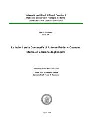
Nell’essere umano, già a partire dal primo anno di vita, viene depositato soltanto
osso lamellare (cosiddetto osso secondario)
che rimpiazza rapidamente i residui di osso
fibroso (cosiddetto osso primitivo, o
primario). Si può osservare che, col
progredire dell’età dell’individuo, si assiste
ad una perdita progressiva di tessuto osseo,
con riduzione della massa ossea totale che
causa la patologia, nota in medicina come
osteoporosi, che determina un maggiore
infragilimento delle ossa le quali divengono
suscettibili a fratture spontanee o a traumi di
modesta entità [ 18 ].
Molti studi sono stati compiuti nel tentativo
di definire l’origine di tale fenomenologia;
Figura 1: Schematizzazione dei
meccanismi cellulari caratterizzanti il
rimodellamento osseo
nel diciannovesimo secolo il chirurgo Julius Wolff ha affermato: “la forma dell’osso
segue la funzione“ intendendo che l’architettura dell’osso è influenzata dagli stress
meccanici associati al suo normale funzionamento [ 19 ] e che l’attivazione dei
meccanismi di formazione di osteoclasti e osteoblasti che determinano il
rimodellamento dell’osso si realizza in presenza degli sforzi mentre laddove il
carico non è applicato si verifica un fenomeno di riassorbimento osseo [ 20 ].
Successivamente egli ha mostrato che la formazione dell’osso incrementa nelle
zone di compressione mentre diminuisce nelle zone soggette a tensione [ 21 ]. Da
qui la definizione delle leggi di Wolff riassunta dalle seguenti tre leggi qualitative:
1) il rimodellamento osseo è governato da sollecitazioni flessionali, non dagli
sforzi principali;
2) il rimodellamento osseo è stimolato da carichi dinamici ciclici, non da
carichi statici;
3) la flessione dinamica produce una crescita ossea nella zona in cui la
flessione causa la concavità [ 16 ];
Esse esprimono il fatto che a seguito dell’applicazione di un carico ottimale, la
formazione di nuovo osso prevale sul riassorbimento, mentre laddove le
condizioni di carico non risultino adeguate, in quanto troppo modeste o
eccessivamente elevate, il meccanismo di riassorbimento risulta dominare su
quello di deposizione ossea [ 22 ]. E’ evidente che la conoscenza di tali
meccanismi non è del tutto ultimata come dimostrano tanti elementi di studio che
non trovano ancora una chiara collocazione. Ad esempio ricerche compiute negli

16 - CAPITOLO 1
anni 50, ad opera dello scienziato Iwao Yasuda, sottolineano il ruolo che
possono avere, in tali meccanismi, le proprietà piezoelettriche dell’osso; esse sono
attribuibili al fatto che, quando è applicato uno sforzo meccanico su una struttura
fortemente anisotropa quale quella del tessuto osseo, esso genera un impulso
elettrico che stimola gli osteociti a registrare, attraverso correnti piezoelettriche, le
sollecitazioni sulla parte di lamella ossea interessata dal carico fino a costruire una
struttura ossea adeguata alle funzioni meccaniche richieste [ 23 ].

L’OSSO NATURALE - 17
1.4 RELAZIONI TRA STRUTTURA E PROPRIETA’
L’osso presenta una struttura piuttosto complessa organizzata secondo cinque
livelli gerarchici differenti definiti in relazione alle unità di riferimento prescelte.
In particolare si distinguono:
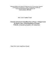
Figura 2: Organizzazione strutturale dell’osso[ 25 ]
I) livello macrostrutturale (~ mm)
II) livello microstrutturale ( 10 - 500µm )
III) livello sub-microstrutturale ( 1 –10µm)
IV) livello nanostrutturale ( 0.1 – 1 µm )
V) livello sub-nanostrutturale. ( 10-3µm )
A livello macrostrutturale l’osso lamellare, che costituisce la quasi totalità dello
scheletro umano, presenta due tipologie di strutture:
a) tessuto osseo spugnoso quando i sistemi lamellari sono organizzati in
trabecole che si intersecano disordinatamente.
b) tessuto osseo compatto quando invece i sistemi di lamelle si compattano
ordinatamente nello spazio[ 25 ].
La distribuzione di tali tipologie di tessuto varia in funzione del tipo di osso che si
prende in esame. In generale nelle ossa lunghe si riconosce una parte centrale
lunga e cilindrica percorsa da un canale e formata da tessuto osseo compatto
(diafisi) e da due estremità più larghe (epifisi) costituite prevalentemente da osso
spugnoso.

18 - CAPITOLO 1
Nelle ossa piatte invece, in cui lo spessore è di un
ordine di grandezza inferiore rispetto alle altre
dimensioni, possiamo distinguere due lamine
superficiali di osso compatto separate da uno strato
di osso spugnoso. Infine nelle ossa corte si riscontra
tessuto essenzialmente spugnoso ricoperto da sottile
strato di osso compatto o di cartilagine [ 16 ].
L’osso compatto o corticale (fig.3) ha un
comportamento anisotropo, presenta cioè maggiore
resistenza alle forze applicate secondo il suo asse
verticale e ha una densità di 1,8 g/cm3 [ 25 ].
L'osso trabecolare o osso spongioso
spugnoso (fig.4) è organizzato in
trabecole, prevalentemente orientate in
senso perpendicolare tra loro; le
trabecole verticali sono più grosse e
sopportano il carico, le trabecole
orizzontali, invece, stabilizzano le
verticali. Le trabecole, così disposte,
formano le cavità in cui è collocato il
midollo osseo. Ne deriva che la sua
densità è inferiore a quella dell’osso
corticale e può variare tra 0,1 ed 1 g/cm3 Figura 4: Osso spongioso [ 24 ]
[ 26 ].
Si osserva che una simile architettura è tutt'altro che casuale in quanto le
trabecole sono conformate secondo l'andamento delle linee isostatiche (quelle
direzioni lungo cui sono dirette esclusivamente tensioni normali e pertanto l’osso
risulterà semplicemente teso o compresso) corrispondenti alla sollecitazione
prevalente a cui sono sottoposte [ 28 ].
Figura 3: Osso corticale [ 24 ]

Figura 5: a) Osso corticale[ 27 ]
b) Osso trabecolare [ 27 ]
L’OSSO NATURALE - 19
Si riportano, a tal proposito delle tabelle che raccolgono i valori medi delle
proprietà meccaniche principali dell’osso; in alcuni casi (tab.1) viene riportato sia
il valore del carico longitudinale che trasversale per mettere in evidenza, anche
numericamente, la forte anisotropia che caratterizza il tessuto:
Caratteristiche strutturali Corticale Spongioso
Fraz. volumetrica ( mm 3 /mm 3 ) 0.90 (0.85 - 0.95) 0.20 (0.05 - 0.60)
Superficie/Volume ( mm 2 /mm 3 ) 2.5 20
Volume totale ( mm 3 ) 1.4 x 10 6 0.35 x 10 6
Superficie interna ( mm 2 ) 3.5 x 10 6 7.0 x 10 6
Tabella 1: Alcune caratteristiche strutturali dell’ osso corticale e spongioso [ 26 ]
Tipo di osso Direzione
della
prova
Ossa arto inferiore
femore
tibia
Perone
Ossa arto superiore
omero
radio
ulna
Vertebre
cervicale
Longitud.
״
״
״
״
״
״
lombare
״
Cranio tangenz.
radiale
Modulo di
elasticità
[GPa]
17,2
18,1
18,6
17,2
18,6
18,0
0,23
0,16
-
-
Sforzo a
rottura per
Trazione
[MPa]
121,0
140,0
146,0
130,0
149,0
148,0
3,1
3,7
25,0
-
Sforzo a
rottura per
compressione
[MPa]
167
159
123
132
114
117
10
5
-
97
Tabella 2: Proprietà meccaniche dell’osso in funzione della propria collocazione nel corpo
umano [ 16 ][ 29 ]

20 - CAPITOLO 1
Il suo comportamento può essere descritto in termini di proprietà strutturali
attraverso la valutazione degli stress globali sul sistema costituito dalle trabecole
più i pori, oppure in termini di proprietà materiali in riferimento alle proprietà
intrinseche delle sole trabecole, in modo da valutare solo gli stress locali ed
ottenere informazioni circa il riassorbimento dell’osso in prossimità di un
impianto [ 30 ].
In generale la distinzione tra osso corticale ed osso spongioso è fatta in relazione
alle variabili di porosità e di densità apparente (definita come il rapporto tra la
massa ed il volume complessivo compresi i pori).
Figura 6: Andamento delle curve σ-ε nel caso di osso
corticale e di osso trabecolare [ 31 ]
Infatti risulta evidente che l’osso trabecolare, meno denso e più poroso dell’osso
corticale, nonché di più giovane formazione, mostra delle proprietà meccaniche,
ed in particolare una rigidità, sensibilmente più basse dell’osso corticale [ 25 ].
E’ necessario sottolineare che tali valutazioni si riferiscono per lo più a proprietà
tensili per le quali si riesce ad ottenere una buona uniformità di risultati.
Le problematiche si complicano nello studio delle proprietà a compressione in
quanto i test da effettuare possono evidenziare problemi di trasferimento del
carico, specie per campioni molto piccoli, in virtù di fenomeni di frizione insorti
tra il piatto della macchina e il materiale [ 33 ].
A livello microstrutturale l’osso presenta elementi strutturali piani, le lamelle,
costituite da fibre di collagene mineralizzato parallele tra loro, riunite a formare le
fibrille, che si sistemano in modo planare (dimensioni di 3-7 µm) o stratificano
(circa 7-8 lamelle) lungo un canale centrale, il canale di Havers, dando vita a
strutture concentriche con dimensioni di 200-300µm (osteoni) [ 25 ].
La notevole anisotropia delle proprietà meccaniche è dovuta, in primo luogo, alla
diversa orientazione che presentano gli osteoni all’interno della struttura rispetto
alla direzione di applicazione del carico; inoltre esse variano anche da un osteone
ad un altro in relazione al diverso contenuto minerale presente nelle lamelle [ 34 ].

L’OSSO NATURALE - 21
Figura 7: Schema della struttura a livello micrometrico e nanometrico: fibrille di collagene
intervallate da cristalli di apatite [ 25 ]
A livello nanostrutturale (≅1-100µm) l’osso si presenta costituito essenzialmente
da cristalli di apatite di dimensioni 2-3µm che vanno a collocarsi negli interstizi,
formatisi tra le fibrille di collagene impacchettate, di dimensioni variabili tra 1-
100µm. La loro forma per lo più appiattita deriva dal fatto che il loro
accrescimento è vincolato ad avvenire lungo l’asse delle fibrille stesse [ 25 ]. Ad
essi si aggiungono proteine non collageniche di varia natura come le
Sialoproteine che regolano la dimensione e l’orientazione di tali cristalli in
quanto adibiti a controllare le riserve di calcio dell’organismo.
Innanzitutto è evidente che al crescere del contenuto di cristalli, e quindi della
sostanza minerale, aumenta la densità dell’osso e, di conseguenza, cresce il
modulo elastico e la rigidità mentre diminuisce la tenacità e la resistenza a
flessione dell’osso [ 16 ] come riassunto nella tabella seguente:
Tipo di osso
Minerale
% in peso
Densità
(g/cm 3 )
Energia di
rottura
(J /m 2 )
Resistenza a
flessione
(Mpa)
Modulo
elastico
(Gpa)
Corno di cervo 59.3 1.86 6190 179 7.4
Femore bovino 66.7 2.06 1710 247 13.5
Osso timpanico di balena 86.4 2.47 200 33 31.3
Tabella 3: Proprietà di differenti ossa animali in relazione al contenuto di minerale [ 16 ]

22 - CAPITOLO 1
Un ruolo importante nelle proprietà meccaniche è svolto dalle fibre di collagene e
in particolare dall’interazione delle fibre collagene di tipo I, che costituiscono la
fase organica, con la fase inorganica costituita essenzialmente da cristalli di apatite
[ 32 ].
A tal proposito sono stati introdotti alcuni modelli micromeccanici (Katz 1971,
Mammone, Hudson 1993) per descrivere le proprietà micromeccaniche dell’osso in
relazione alla composizione molecolare; l’idea è quella di immaginare l’osso come
un composito molecolare costituito da collagene di tipo I e apatite come
schematizzato nella figura seguente (fig.8):
Figura 8: Sezione longitudinale e trasversale di una
fibrilla di collagene - Redrawn from Glimcher (1976)
[ 33 ]
Inizialmente gli interstizi tra la molecole di collagene sono occupati da sostanza
fisiologica, la quale lascia gradualmente il posto ai cristalli di apatite a seguito
dell’attivazione del processo di mineralizzazione dell’osso. Tale processo
prosegue trasformando il tessuto osseo soffice e flessibile in un materiale denso e
rigido con proprietà prossime a quelle dei metalli leggeri.
Studiando il materiale composito, è possibile stimare il modulo elastico
longitudinale attraverso:
E = E V + E V
m
dove Em, Ec, Vm, Vc sono rispettivamente i moduli elastici e le frazioni
volumetriche dell’ idrossiapatite e del collagene; Tenendo conto che risulta:
V
E
m
m
⋅V
E
c
c
m
c
< 100
< 100
c

L’OSSO NATURALE - 23
si ricava che il massimo contributo del collagene alla rigidezza dell’osso è
inferiore all’1% [ 32 ].
Molto importante risulta poi l’orientamento delle fibrille rispetto alla direzione di
applicazione del carico. Le fibrille, ottenute da singole fibre di collagene (dalla
caratteristica forma a triplice elica), sono tenute insieme da crosslinks e legami a
ponte di idrogeno; esse sono costituite da aminoacidi, molecole fortemente non
polari, e pertanto tendono ad interagire preferibilmente con se stesse piuttosto
che con molecole di acqua favorendo così la formazione delle fibrille. Al
diminuire della concentrazione di crosslinks diminuisce la rigidità e soprattutto la
tenacità del materiale intesa come la sua capacità di assorbire energia prima della
rottura mentre il modulo elastico resta all’incirca invariato.
Una forte variazione del modulo elastico è invece fortemente correlata alla
presenza di molecole di acqua nel tessuto; infatti la presenza di gruppi idrofillici
lungo la catena gioca un ruolo importante in quanto permette il raggiungimento
della stabilità delle molecole e favorisce l’allineamento delle catene riducendo il
modulo elastico dell’osso e migliorando invece la sua adattabilità ai carichi [ 31 ].
Proprietà del collagene Wet Dry
Upper Tensile Stress ( Mpa ) 2 - 40 20 - 360
Modulo Trazione E ( Mpa ) 10 - 570 2100 - 2700
Deformazione rottura (%) 6 - 48 11-17
Tabella 4: Proprietà meccaniche del collagene [ 34 ]

24 - CAPITOLO 1
1.5 STATI DI SOLLECITAZIONE DELL’OSSO
Le ossa, durante la loro attività giornaliera, sono sottoposte a varie tipologie di
sollecitazioni meccaniche (trazione, compressione, piegamento, taglio, torsione
etc.).
In realtà, nell’organismo vivente, tutte le sollecitazioni possono intervenire
contemporaneamente, il che rende piuttosto difficoltosa una modellazione teorica
dello stato di sollecitazione in grado di riprodurre quantomeno fedelmente i
comportamenti reali[ 31 ]. Si riportano i tipi di sollecitazione caratteristici delle
ossa :
I. trazione: in tal caso due carichi uguali ed
opposti sono applicati alle estremità del
tessuto verso l’esterno, in modo tale che
all’interno della struttura risulti una
distribuzione uniforme di forze diretta
lungo l’asse di applicazione dei carichi. In
queste condizioni la struttura si allunga in
direzione assiale e si assottiglia lungo le altre
due direzioni.
II. compressione: carichi uguali e opposti sono applicati alle estremità dell’osso,
ma stavolta diretti verso l’interno: anche in
questo caso si osserva, all’interno della
struttura, una distribuzione uniforme di
forze, su un piano perpendicolare alla
direzione di applicazione del carico, che
determina un accorciamento in direzione
assiale ed un allargamento del corpo in
direzione radiale. La valutazione delle
sollecitazioni a compressione è molto importante in quanto esse sono spesso
la causa di fratture, ad esempio, nelle vertebre, in soggetti affetti da patologie
degenerative del tessuto osseo quali
l’osteporosi.
III. Carichi in direzione di taglio: viene
applicata una tensione parallelamente alla
superficie della struttura. Ne risultano
forze di taglio e tensioni all’interno della
struttura. La forza di taglio può essere
pensata come una distribuzione di forze che agisce sulla superficie della

L’OSSO NATURALE - 25
struttura su un piano parallelo a quello in cui è applicato il carico. Una
struttura sottoposta a una sollecitazione di questo tipo si deforma
internamente: immaginando di prendere due
fibre di materiale, la deformazione porta ad un
cambiamento dell’angolo compreso tra queste.
In particolare forze di taglio possono essere
presenti nel caso in cui ci sia l’azione sia di
sollecitazioni a trazione che a compressione. In
vivo, fratture dovute a forze di taglio si osservano principalmente nell’osso
spugnoso.
IV. Flessione: In questo caso, i carichi sono applicati in modo che la struttura
subisca una curvatura lungo il proprio asse. Il campione, in questo modo, è
sottoposto a sforzi sia di trazione che di
compressione.
Dal momento che un osso non ha una
struttura omogenea, le tensioni non sono
distribuite in modo simmetrico. Un
piegamento può essere ottenuto mediante
l’applicazione di tre o quattro forze (in tal
senso possono essere realizzate prove di flessione a tre o a quattro punti).
sollecitazioni flessionali sono tipiche di fratture in particolare nelle ossa
lunghe (tibia, femore, ossa del braccio).
V. Torsione: il carico è applicato in modo così da ottenere
una rotazione attorno ad un asse, e all’interno della
struttura si ottiene una coppia: in questo caso le forze di
taglio sono presenti sull’intero sistema.
VI. carichi combinati: Solo teoricamente è possibile
pensare ad un osso sottoposto a un singolo tipo di
sollecitazione come quelle viste in precedenza;
normalmente, anche nei movimenti che appaiono più semplici, le ossa, in un
organismo vivente, subiscono sollecitazioni più complesse.
Tali sollecitazioni combinate a cui sono sottoposte le ossa dipendono anche da
molteplici fattori di diversa natura [ 34 ]:
- l’azione dei muscoli, la quale può produrre tensioni di compressione che
sono in grado di compensare (parzialmente o totalmente) forze di trazione cui
è sottoposto l’osso; questa capacità di compensazione si riduce con
l’aumentare dell’affaticamento del muscolo.

26 - CAPITOLO 1
- la velocità di applicazione del carico dal momento che l’osso è un
materiale viscoelastico.
Nel seguente diagramma è mostrato il differente comportamento di una
porzione di osso corticale sottoposto a carichi applicati con diversa velocità.
Questo fattore è importante poiché influenza il modo in cui un osso subisce
una frattura, e, di conseguenza, condiziona il grado di danneggiamento dei
tessuti molli circostanti. In particolare, se la velocità di carico è bassa, l’energia
immagazzinata nell’osso si può
dissipare in un'unica rottura (e i
tessuti circostanti rimangono
intatti) in quanto la risposta del
materiale risente in maniera
proporzionale con la velocità di
carico della presenza delle fibre di
collagene che riducono la rigidezza
(in quanto abbassano il modulo
elastico complessivo) ma ne
aumentano la tenacità.
Al contrario se la velocità di carico
è alta, l’energia si dissipa in fratture
multiple, provocando la
formazione di numerosi frammenti
in grado di rovinare anche i tessuti
circostanti il segmento osseo.
Figura9: Differente risposta dell’osso in
relazione alla velocità di carico: all’
aumentare della frequenza di carico
aumenta il modulo elastico [ 31 ] [ 34 ]
Tale comportamento è dovuto ad una risposta di natura fragile dovuta alla
maggior incidenza della componente minerale di idrossiapatite nella risposta
meccanica del tessuto osseo naturale.
- la ripetitività con cui un carico è applicato all’osso (carichi ciclici): le
fratture, oltre ad essere provocate da un carico maggiore rispetto della
massima tensione sopportata del tessuto, possono essere originate
dall’applicazione ripetuta di carichi di minore intensità e comunque al di sopra
di un certo valore di soglia legato alla natura del materiale ed alla sua
resistenza a fatica. In particolare esperimenti compiuti su campioni di ossa in
vitro, hanno permesso di osservare che l’applicazione ripetuta di piccoli
carichi è sempre causa di microfratture che, mediamente, in un soggetto
normale vengono riassorbite mediante processi di rimodellamento osseo.

L’OSSO NATURALE - 27
Solo in caso di frequenze di carico troppo elevate tali microfratture possono
essere degenerative in quanto i processi fisiologici di rimaneggiamento osseo
non sono in grado di ripararle adeguatamente [ 34 ].
- La geometria dell’osso: la morfologia e le dimensioni delle ossa influenzano
significativamente la risposta meccanica del tessuto; ad esempio il carico a
rottura (nel caso di sforzi a compressione e a trazione) e la rigidità di un
segmento osseo sono proporzionali alla sezione dell’osso stesso nel senso che
ad una sezione maggiore corrisponde un osso più rigido e più resistente.
Anche la lunghezza dell’osso influenza le proprietà meccaniche dell’osso
soprattutto in risposta alle sollecitazioni flessionali e, in tono minore, in
risposta agli sforzi a compressione a seguito dell’accentuarsi dei problemi di
svergolamento.
- L’età del soggetto: infatti con l’aumentare degli anni si riduce la densità
dell’osso. Ciò determina un progressivo assottigliamento nell’osso corticale,
una riduzione generale della massa nell’osso trabecolare, a seguito
dell’assottigliamento delle trabecole longitudinali e del riassorbimento di
quelle trasversali.
Ad esempio nel 1990 Mosekilde studiando il corpo vertebrale ha riscontrato,
in funzione all’incremento dell’età, una perdita nella continuità delle trabecole
e, in particolare, una perdita delle trabecole ad orientamento orizzontale.
Questo specifico mutamento nell’architettura trabecolare lascia presagire una
futura riduzione della rigidezza e della resistenza ossea con l’età.
Una perdita di continuità e di elementi strutturali può essere la causa di
fratture locali associate alla formazione di microcalli. Mosekilde sulla base di
sperimentazioni condotte su vertebre lombari ha osservato in soggetti con età
nell’intervallo tra 18-85 anni una riduzione progressiva del modulo elastico E
del 17%, per decade, in direzione assiale. In concomitanza è stata osservata
una riduzione della resistenza alla rottura stimata del 6%, per decade, ed un
notevole incremento dell’anisotropia dell’architettura trabecolare [ 31 ].

28 - CAPITOLO 2
2. INGEGNERIA DEI TESSUTI
2.1 DEFINIZIONE
L’ingegneria dei tessuti è quella disciplina che indaga sulle relazioni tra funzioni e
struttura nei tessuti sani o caratterizzati da patologie degenerative, nel tentativo di
ripristinare il loro funzionamento originario (Skalak e Fox, 1989)[ 36 ].
Traendo le sue origini dagli studi pionieristici di elettrofisiologia avviati da
Galvani e Volta nel XIX° secolo, la sua nascita ufficiale risale alla seconda metà
del secolo scorso, alla fine degli anni 80, quando, presa piena coscienza delle
nuove tecnologie di indagine medica (tomografie, risonanze magnetiche ed
ultrasoniche, etc.) scoperte negli anni 70, alcuni gruppi di scienziati, afferenti da
diversi campi della scienza, come la biologia, la medicina, la chimica, l’ingegneria,
intuirono la necessità di fondere le proprie conoscenze al fine di realizzare sistemi
che, imitando la natura, fossero in grado di sostituire in maniera permanente
porzioni localizzate o interi tessuti all’interno dell’organismo [ 37 ].
Dunque l’ingegneria dei tessuti è un settore scientifico molto giovane ma in pieno
sviluppo ed in costante e progressiva evoluzione, così vasto da fare riferimento a
molteplici applicazioni che abbracciano svariati settori della bioingegneria e non
solo.
Il termine Tissue engineering è stato introdotto per la prima volta dagli
organizzatori del I st congress NSF tenutosi sul lago di Tahoe nel 1988 per
identificare “l’insieme dei principi e dei metodi delle scienze mediche ed
ingegneristiche atti a stabilire le relazioni fondamentali tra struttura e funzioni di
tessuti sani o patologici di mammiferi”[ 2 ].
Nel tempo il concetto di ingegneria dei tessuti ha subito molteplici modifiche che
ne hanno arricchito e perfezionato continuamente la definizione.
In questo ottica sono riportate nel seguito le definizioni introdotte dagli scienziati
Langer e Vacanti le quali racchiudono in maniera completa ed esaustiva i
principi essenziali sui quali si fonda l’ingegneria dei tessuti:
“La tissue engineering è quel settore interdisciplinare che applica i principi
dell’ingegneria e delle scienze che studiano la vita per lo sviluppo di sistemi in
grado di restituire, conservare e migliorare le funzioni del tessuto” (Vacanti 1995);
“Il suo obiettivo primario è quello di ripristinare le funzionalità dei tessuti
mediante l’impianto di elementi “viventi” che siano in grado, in tempi
clinicamente accettabili, di diventare parte integrante dell’organismo in cui
vengono introdotti, con ridotti margini di insuccesso postimpianto” (Langer 1999)
[ 2 ] [ 41 ].

2.2 TAPPE EVOLUTIVE
L’INGEGNERIA DEI TESSUTI - 29
Negli ultimi decenni, a partire dalla seconda metà del secolo scorso, la cura di
anomalie congenite e di traumi caratterizzanti tessuti dell’organismo umano è
stata realizzata attraverso l’impiego di tessuti donatori i quali una volta impiantati
fossero in grado di ripristinare la funzione del tessuto compromesso.
In particolare, nell’ambito delle tecniche di sostituzione ed integrazione di
porzioni di tessuto osseo mancanti o danneggiate, sono state introdotte svariate
metodologie alcune delle quali, pur essendo obsolete in relazione alle attuali
conoscenze scientifiche, costituiscono, ancora oggi, una risorsa importante per la
cura di difetti scheletrici derivanti da malformazioni o traumi in quanto regolate
da procedure rigidamente standardizzate che ne assicurano la riuscita con piccoli
margini di insuccesso [ 1 ].
A seconda dell’applicazione a cui si fa riferimento, delle motivazioni che
inducono alla sostituzione del tessuto nonché in relazione all’entità dell’intervento
possono essere adottate diverse soluzioni:
1. Innesto di protesi artificiali di materiale inorganico :
Tale tecnica si fonda essenzialmente sull’impiego di materiali metallici e ceramici,
di largo utilizzo nel settore della biomedica
negli ultimi decenni del secolo scorso, per la
realizzazione di sistemi protesici (es. protesi
d’anca) che, una volta impiantati, siano in
grado di sostituire in maniera completa e
definitiva il tessuto naturale simulandone il
comportamento meccanico senza però
determinare alcuna alterazione dell’ambiente
articolare in cui è introdotto. Tale soluzione
presenta in realtà numerosi problemi:
• limitata durata e affidabilità di alcuni
materiali una volta impiantati nel
paziente;
Figura 10: Confronto tra la risposta
meccanica a trazione dell’osso e quella
di un metallo e di un vetro [ 16 ]
• ridotta biocompatibilità del materiale, quindi elevata probabilità di
infezioni di varia natura e alto rischio di rigetto;
• differenze, in alcuni casi significative, della risposta meccanica dei metalli
rispetto al tessuto sostituito (soprattutto nel confronto dei moduli
elastici) come si può evincere dal diagramma puramente qualitativo a
lato (Fig.10):

30 - CAPITOLO 2
• necessità di rimozione e sostituzione della protesi, anche più di una volta
dopo l’impianto, a seguito dell’accrescimento fisiologico che mostrano i
tessuti circostanti (Tale aspetto è certamente di maggiore rilevanza nel
caso di pazienti di giovane età);
• ricrescita impropria del tessuto osseo in corrispondenza della zona di
giunzione con la protesi con conseguente la formazione di “calli ossei“
intorno alle viti impiegate per il fissaggio della protesi all’interfaccia con i
tessuti circostanti [ 16 ][ 38 ];
2. Tecniche di autoinnesto di materiali fisiologici (autografts).
Tale tecnica consiste nell’impianto di un tessuto o di un organo in una nuova
locazione all’interno dello stesso individuo. Esempi comuni di auto trapianto
sono l'uso della safena per eseguire il by-pass coronarico o l'utilizzo di pelle del
paziente stesso in caso di ustioni. Questo sistema presenta numerosi vantaggi
rispetto alla soluzione precedente pur non essendo ancora la soluzione ideale. I
principali vantaggi sono:
• maggior stabilità e durata del materiale;
• elevata biocompatibilità e impossibilità di fenomeni di rigetto dal
momento che il tessuto è autogeno;
• possibilità di un “normale” sviluppo del tessuto innestato seguendo la
naturale crescita dei tessuti circostanti (possibilità di impianti anche per
pazienti in età pediatrica senza necessità di ulteriori interventi).
Nonostante tali aspetti notevolmente significativi sono comunque molte le
problematiche associate ad una tale tipologia di trapianto:
• un intervento di questo tipo può essere eseguito solo su un ridotto
numero di ossa e, nel caso di parti da sostituire di piccole dimensioni in
quanto la disponibilità di tessuto donato dal paziente è certamente di
modesta entità;
• necessità di tecniche e strumentazione di microchirurgia complesse e
costose;
• problemi estetici relativi alla regione da cui è stato prelevato l’osso;
• possibilità di infezioni sia nel sito di prelevamento che in quello di
innesto con conseguente rischio di danneggiamento di entrambe le
parti;
• problemi connessi alla modellazione ed all’adattamento del tessuto
donato all’interno della sua nuova collocazione [ 16 ][ 38 ][ 39 ]

L’INGEGNERIA DEI TESSUTI - 31
3. Tecniche di innesto di materiali fisiologici non autogeni.
La tecnica consiste nell’innesto di tessuti o organi non appartenenti all’individuo
che subisce il trapianto; in particolare quando il trapianto avviene tra individui
della stessa specie, ma non identici geneticamente si parla di Allograft, mentre
nel caso in cui esso avvenga tra individui di specie differenti (ad es. suini, ovini
etc.) si parla di Xenograft [ 16 ].
Questo sistema, in entrambe le sue varianti, permette di risolvere alcuni aspetti
negativi connessi alle due tecniche precedenti.
Infatti non dovendo più operare un prelievo di tessuto osseo dal paziente che
subisce il trapianto risultano totalmente estinti sia i rischi di infezione nelle zone
di prelevamento del tessuto sia gli inestetismi legati all’assenza di tessuto in
corrispondenza di essi. Ma soprattutto risultano quasi totalmente risolti i
problemi legati alla reperibilità del materiale da innestare con la conseguente
possibilità di sostituire, quindi, anche segmenti ossei di dimensioni maggiori.
A tali vantaggi vanno aggiunti anche una serie di aspetti notevolmente critici che
impediscono la realizzazione del trapianto se non in particolari circostanze; In
particolare si riscontrano:
• persistenti problemi di rigetto;
• possibilità di infezioni nel sito di innesto e rischio di trasmissione di
patologie di varia natura al paziente (nonostante i rigorosi controlli previsti
dalle leggi vigenti riguardo il tessuto da trapiantare).
• Elevati costi dovuti alle strumentazioni nonchè alle tecniche chirurgiche [ 16
][ 38 ].
In quest’ottica risulta evidente la necessità di incentivare lo sviluppo di nuove e
migliori tecniche che permettano di eliminare, o quantomeno ridurre al minimo,
l’incidenza dei problemi connessi alle tecniche di innesto preesistenti.
Negli ultimi anni, a seguito di un intensa sinergia tra diversi settori della
bioingegneria e della biomedicina, molte soluzioni sono state avanzate in
alternativa all’utilizzo di tessuti donatori; in questo senso è stata introdotta una
vera e propria classificazione che prevede all’interno del settore del tissue
engineering la distinzione di due grosse aree [ 40 ]:
1. Organ substitution alla quale afferiscono tutte le tecniche di
trapianto che sono state finora descritte;
2. Tissue regeneration: alla quale afferiscono le moderne ricerche
mirate alla ricostruzione parziale o totale dei tessuti danneggiati
mediante la realizzazione di strutture di supporto tridimensionali nelle
quali possano aderire e proliferare le cellule.

32 - CAPITOLO 2
2.2 TISSUE REGENERATION
La Tissue Regeneration è l’area dell’ingegneria dei tessuti orientata alla
ricostruzione dei tessuti mediante l’impiego di strutture di supporto
ingegnerizzate costituite da materiali di nuova concezione [ 41 ]. Le strategie da
essa seguite sono caratterizzate dalle seguenti fasi di sperimentazione (Langer,
1999):
I.Scelta delle cellule da
impiantare: esse devono
essere identificate, isolate e
moltiplicate in maniera
sufficiente per la
proliferazione in vivo.
II.Realizzazione di substrati
(sistemi aperti, sistemi chiusi)
su cui depositare le colonie
cellulari: progettazione dei
materiali, della struttura e
della geometria.
III.Coltivazione in vitro: le
cellule sono uniformemente
distribuite sul substrato e
lasciate crescere in ambiente
fisiologico simulato all’interno
di un bioreattore.
IV.Impianto in vivo: la struttura
ingegnerizzata, caricata con le
cellule, viene collocata nel sito
di interesse al fine di ottenere
un integrazione ottimale con i
tessuti circostanti [ 42 ].
Figura 11: Schema rappresentativo delle fasi di
sperimentazione che caratterizzano la tissue
regeneration [ 43 ]
Nei paragrafi successivi verranno brevemente approfondite le diverse fasi della
tissue regeneration sorvolando sulla fase relativa alla realizzazione dei substrati la
quale verrà ampiamente discussa nel capitolo successivo.

2.3 LE CELLULE
Le cellule costituiscono, accanto ai materiali che
costituiscono i substrati, la materia prima alla
quale si attinge nella tissue regeneration. Al loro
interno esse presentano una struttura ben
definita caratterizzata da un nucleo centrale
all’interno del quale è conservato il corredo
cromosomico che definisce il patrimonio
genetico (genoma) della cellula.
Esternamente essa è rivestita da una membrana
cellulare costituita da molecole lipidiche rivolte
con la loro estremità idrofillica verso la matrice
extracellulare esterna [ 44 ].
All’interno del corpo umano sono presenti
diverse tipologie di cellule, circa 200, tra loro
differenti, aventi tutte lo stesso contenuto
genetico, ma una differente programmazione
della propria attività genetica. In altri termini le
cellule sono “differenziate” in relazione alla
presenza di proteine regolatrici presenti
all’interno del loro corredo proteico in grado di
L’INGEGNERIA DEI TESSUTI - 33
A membrana cellulare
B citoplasma
C vacuoli
D nucleo
E membrana nucleare
F cromosomi
G mitocondri
H inclusioni varie
I reticolo endoplasmatico
J nucleolo
K centrosoma
L corpo del Golgi
Figura 12: Rappresentazione di
una cellula in sezione[ 44 ]
attivare solo alcune funzioni del patrimonio genetico. Il processo che porta alla
definizione dei diversi tipi di cellule è noto come “differenziamento”.
Parallelamente ad esso sono attivi i processi di riproduzione cellulare necessari alla
loro proliferazione: essi sono tanto più favoriti quanto le cellule sono meno
differenziate (da qui il motivo per cui le cellule staminali, che sono le cellule ab
origine dell’organismo di ciascun essere vivente, sono quelle più adatte alla
coltivazione per la realizzazione di nuovi tessuti).
Sia i meccanismi di differenziamento che quelli di riproduzione cellulare sono alla
base della prima fase della tissue regeneration; ovviamente, nel caso della
rigenerazione dei tessuti, la problematica è resa più complessa dalla presenza del
substrato solido: la proliferazione cellulare infatti risulta condizionata in maniera
significativa dalla più o meno favorevole adesione delle cellule al substrato; in
questo senso vanno scelti opportunamente i polimeri impiegati per la
realizzazione della struttura di supporto; inoltre solitamente è utile somministrare
delle proteine transmembrana in grado di riconoscere proteine extracellulari
(fibronectina, etc.) agevolando in questo modo l’adesione cellula/substrato [ 43 ].

34 - CAPITOLO 2
Nell’ambito della tissue regeneration possono essere impiegate tipologie diverse
di cellule in relazione al tipo di tessuto che ci si propone di riprodurre.
Nel caso specifico dell’ingegneria del tessuto osseo al quale fa riferimento in
questo lavoro di ricerca, si procede all’utilizzo di osteoblasti le quali sono cellule
giovani e molto attive derivanti da cellule mesenchimali presenti nel tessuto
connettivo [ 44 ].
2.4 COLTURE IN VITRO: BIOREATTORI
Nella tissue regeneration le colture cellulari risultano più difficili da realizzare
rispetto alle monocolture cellulari tradizionali in quanto condizionate dalle
interazioni con la struttura tridimensionale che le contiene. Infatti all’interno del
substrato 3D le condizioni di accessibilità alle cellule da parte dei fluidi biologici
risultano molto sfavorite rispetto al caso di cellule deposte lungo un substrato
piano (film sottili e membrane 2D); in particolare alcuni studi hanno dimostrato
che, nel caso di coltura statica in 3D l’indice di vitalità cellulare all’interno dello
scaffold risulta essere molto inferiore a quello lungo le superfici.
Infatti, grazie al continuo ricambio del terreno di coltura, da un lato, si consente il
mantenimento della concentrazione dei nutrienti intorno ad un valore costante e
dall’altro si favorisce la liberazione del mezzo dai residui derivanti dal
metabolismo cellulare [ 46 ]. Ne consegue che l’organizzazione 3D delle cellule
ossee è cruciale per la formazione di tessuto in vivo e che il fenotipo di cellule
seminate dipende dall’organizzazione strutturale della matrice [ 47 ][ 48 ]. Inoltre
la coltura di cellule in vitro risponde ad un insieme di parametri legati alla
stimolazione meccanica quali le condizioni di flusso del mezzo di coltura, la
pressione idrostatica la deformazione del substrato [ 10 ].
In particolare, correnti studi hanno dimostrato che le condizioni in flusso
incidono significativamente sul comportamento delle cellule dell’osso [ 49 ][ 50 ]
in quanto intervengono su molteplici fattori biochimici quali il calcio
intracellulare, l’ossido nitrico, la prosteoglandina E2, sui fattori di trascrizione
intracellulari nonché sull’espressione di alcuni geni.
La stimolazione meccanica indotta dalle condizioni di flusso sulle cellule ossee in
vitro consente di mimare abbastanza fedelmente la risposta fisiologica del tessuto.
Al contrario il gradiente di pressione relativo ai carichi fisiologici associati alla
locomozione, produce principalmente una deformazione della matrice ossea
mineralizzata. In particolare, spingendo la componente fluida della matrice
extracellulare verso l’esterno della corteccia ossea attraverso i canalicoli lacunari,
esso gioca un ruolo sostanziale nei meccanismi di formazione e di riassorbimento

L’INGEGNERIA DEI TESSUTI - 35
del tessuto osseo nonché interviene sui meccanismi di produzione delle proteine
che regolano la fase minerale del tessuto.
Infine a ciò si aggiunge, come rilevato da alcuni studi, che l’azione di forze
meccaniche dettate dalle condizioni di flusso presenti all’interno dell’ambiente
extracellulare condizionano fortemente i diversi meccanismi alla base del
funzionamento delle cellule inducendo modifiche sia sulla formazione del
citoscheletro cellulare che nell’interazione tra citoscheletro e matrice
extracellulare. Infatti, lo stress meccanico indotto dalle condizioni di flusso
esterne si trasmette all’interno della cellula mediante il sistema fibroso che
costituisce il citoplasma cellulare alterando la geometria dell’intera cellula la quale
reagisce a tale perturbazione modificando i propri meccanismi di adesione,
proliferazione e differenziazione a danno della crescita del tessuto.
In altri termini il microambiente delle cellule dell’osso è determinato
dall’interazione dinamica tra le sollecitazioni meccaniche agenti sulle cellule attive
e l’architettura della matrice in continuo mutamento [ 43 ].
Per tutti questi motivi le colture cellulari per la rigenerazione dei tessuti non
possono essere realizzate mediante tecniche tradizionali di tipo statico ma è
indispensabile l’impiego di nuove tecniche di coltura che consentono lo sviluppo
cellulare in regime dinamico.
Le tecniche di coltura dinamica si fondano sull’utilizzo del bioreattore, definito
come il dispositivo nel quale si realizzano processi chimici e/o biologici sotto
stretto monitoraggio delle condizioni di prova (pH, temperatura, pressione,
apporto di sostanze nutritive e rimozione delle scorie) in modo da riprodurre
l’ambiente biologico presente all’interno dell’organismo [ 51 ][ 52 ][ 53 ].
Contrariamente a ciò che accade nelle colture in vitro di tipo statico dove il
mezzo di coltura circola all’interno del substrato semplicemente per diffusione
passiva, all’interno di un bioreattore, grazie all’utilizzo di adeguati sistemi di
pompaggio, è possibile istaurare un regime convettivo in grado di favorire la
perfusione del mezzo di coltura all’interno di tutte le cavità del substrato in
maniera ottimale consentendo un’adesione ed una proliferazione cellulare
uniformemente distribuita su tutta la sua superficie [ 44 ].
Il processo di coltura cellulare prevede tre diverse fasi successive:
Semina cellulare: le cellule, incontrando il substrato per la prima volta, hanno la
necessità di aderire ad esso per poi moltiplicarsi; in questa fase, accanto ad una
eccellente compatibilità cellula/substrato, è indispensabile ricreare le condizioni
fluidodinamiche che favoriscano i meccanismi di adesione riducendo al minimo i
fenomeni di mortalità cellulare.

36 - CAPITOLO 2
Coltivazione in vitro: le cellule, una volta aderse alla superficie dello scaffold,
proliferano all’interno della porosità interconnessa riempiendo gradualmente
l’intera struttura.
Coltivazione in vivo: Il costrutto carico in parte di cellule ed in parte di tessuto
in neoformazione, viene impiantato all’interno dell’organismo nella zona di
interesse fino alla completa formazione del tessuto[ 53 ].
Nell’ambito del processo di semina cellulare, attualmente, esistono molteplici
sistemi, propriamente detti bioreattori di semina, i quali consentono di
ottimizzare il processo di adesione cellulare sulle superfici dello scaffold
avvalendosi di differenti principi di funzionamento.
In particolare è possibile distinguere le seguenti cinque differenti tipologie di
bioreattori di semina con particolare riferimento alle più comuni applicazioni per
la tissue engineering [ 52 ]:
I. Spinning flask:
II. Rotating walls
III. Hollow fiber bioreactors
IV. Direct perfusion
V. Stimolazione meccanica
I bioreattori spinner flask consentono l’invasione dello scaffold da parte delle
cellule per convezione; in particolare il mezzo di coltura entrando all’interno di
un contenitore sterile (fig.13) investe la struttura opportunamente vincolata;
l’accesso del mezzo di coltura ed il riempimento efficace della struttura sono
garantite da una miscelazione del mezzo mediante un agitatore posto all’interno
del bioreattore al di sotto dei campioni. Un simile sistema garantisce un eccellente
trasporto di massa ed una elevata efficienza della semina cellulare.
Figura 13; Spinner flask [ 52 ]
Il principale inconveniente di tale sistema risiede nella possibilità di fenomeni di
turbolenza del flusso all’interno del mezzo di coltura che possono determinare
problemi di dedifferenziazione cellulare e ridurre l’accessibilità del mezzo nelle
zone dello scaffold meno raggiungibili.

L’INGEGNERIA DEI TESSUTI - 37
Un’alternativa molto diffusa è offerta dal sistema rotating-walls vessels (fig 14
a,b,c) il quale consente di creare un microambiente di coltura dinamico riducendo
gli sforzi tangenziali ed aumentando la velocità di trasferimento di massa
mediante l’impiego di un dispositivo rotante.
In particolare il dispositivo risulta costituito da una camera rotante rispetto ad un
asse all’interno della quale i campioni vengono lasciati liberi di muoversi: una
volta introdotto il fluido di coltura, a seguito della rotazione, il campione risulterà
sottoposto all’azione di tre forze, una forza di trascinamento Fd tangenziale alla
rotazione, una forza centrifuga Fc diretta verso l’interno ed una forza gravitazione
Fg diretta verso il centro.
L’azione congiunta di queste tre forze determina la diffusione del mezzo di
coltura all’interno della struttura tridimensionale contribuendo efficacemente alla
semina degli scaffold e provvedendo, al contempo, efficacemente al giusto
nutrimento delle cellule nonchè alla rimozione delle scorie prodotte[ 52 ].
Figura 14: Rotating-walls vessels [ 52 ]
La tecnica che attualmente trova maggiori consensi in questo ambito è quella
della perfusione diretta: il dispositivo, costituito da due parti, consente il
passaggio del mezzo di coltura, in condizioni di flusso laminare, attraverso il
campione in direzione assiale; il campione non è libero di muoversi ma è
opportunamente ancorato al sistema mediante una coppia di ganasce solidali alle
due parti del dispositivo stesso.
Un sistema di questo tipo (fig.15), oltre a favorire l’adesione e la proliferazione
cellulare, consente una diffusione cellulare più uniforme con un incremento del
trasporto di massa soprattutto nelle regioni di bulk oltre che nelle zone
periferiche della struttura.
Un sistema di questo tipo, pur avendo a proprio vantaggio anche una facilità di
utilizzo ed un’economicità nella gestione, presenta delle caratteristiche
fluidodinamiche al proprio interno lontane dalle condizioni fisiologiche naturali
che alterano il normale processo di semina.

38 - CAPITOLO 2
Figura 15: Reattore di semina a perfusione diretta (A) e circuito di perfusione (B) [ 54 ]
Il principale limite dei sistemi siffatti è legato al fatto che in essi la semina avviene
in assenza di stimolazione meccanica delle cellule; nel microambiente naturale,
invece, i meccanismi di ricrescita tissutale sono influenzate in maniera rilevante
dalle sollecitazioni meccaniche che agiscono sui tessuti ed in particolare sul
tessuto osseo.
In questa direzione negli ultimi anni sono stati realizzati bioreattori in grado di
ricreare l’ambiente fisiologico sia dal punto di vista fluidodinamico che dal punto
di vista meccanico. In particolare, tale dispositivo (fig.16), mediante un sistema
vite/madrevite, consente di stimolare substrati cellulari a trazione o
compressione e/o a torsione quando sono immersi nel mezzo di coltura durante
il processo di semina e nelle prime fasi di coltura in vitro [ 52 ].
In tal modo esso consente, da un lato, di valutare l’incidenza delle sollecitazioni
meccaniche sull’evoluzione dei meccanismi di adesione e di proliferazione
cellulare, dall’altro di definire i carichi ottimali a cui sottoporre il substrato
durante l’impianto al fine di stabilire i tempi di inattività del paziente durante la
degenza post-operatoria.
Figura 16: Bioreattore di semina a stimolazione meccanica [ 52 ]

3. SCAFFOLDS TRIDIMENSIONALI
SCAFFOLDS TRIDIMENSIONALI - 39
3.1 DEFINIZIONE
Gli scaffolds sono strutture tridimensionali ingegnerizzate aventi la capacità di
sostituire temporaneamente il tessuto naturale favorendo i meccanismi di
differenziamento, di adesione e di proliferazione cellulare[ 55 ].
Essi svolgono principalmente tre ruoli fondamentali:
facilitano la localizzazione ed il rilascio di cellule in parti specifiche del
corpo;
definiscono e mantengono uno spazio tridimensionale per la formazione
dei nuovi tessuti con un’appropriata struttura;
guidano la crescita e lo sviluppo dei nuovi tessuti nonché il flusso delle
sostanze nutritive necessario al loro sostentamento[ 55 ][ 56 ];
Tali strutture devono mostrare, in condizioni ideali, eccellenti doti di stabilità
meccanica, conservando specifiche caratteristiche di compatibilità biologica e
funzionale. In particolare la stabilità meccanica di uno scaffold dipende
primariamente dalla scelta del materiale, dalla sua architettura e dall’interazione
che i suoi materiali costitutivi presentano con le cellule.
La funzionalità biologica, invece, è regolata essenzialmente da segnali di tipo
biologico (ad esempio fattori di crescita), dalla matrice extracellulare (ECM) e
soprattutto dalle cellule circostanti che, da un lato, provvedono al supporto
meccanico e, dall’altro, intervengono nella regolazione dell’attività cellulare [ 55 ][
56 ][ 57 ].
3.2 PROGETTAZIONE DI SCAFFOLDS
Alla luce di quanto affermato, gli scaffolds sono assimilabili a matrici di varia
natura, sia fisica che chimica, atte a sostituire temporaneamente segmenti ossei
del tutto assenti o in condizioni talmente deteriorate da richiedere una completa
ricostruzione del tessuto[ 5 ][ 39 ].
Durante le fasi di progettazione di uno scaffold, in primo luogo, risulta
indispensabile analizzare le principali caratteristiche dei materiali impiegati e la
loro adeguatezza in relazione alle finalità richieste dall’applicazione. In particolare
tali requisiti possono essere tratti dal seguente schema di validità generale nella
tissue regeneration (fig.17).

40 - CAPITOLO 3
Figura 17:
Schema riassuntivo dei paramentri che
intervengono nella progettazione di
scaffolds per tissue regeneration [ 24 ]
Da tale schema si evince la presenza di due insiemi distinti di parametri:
parametri biologici, connessi alla interazione della matrice con le cellule
con cui essa viene a contatto;
parametri ingegneristici connessi alla funzionalità meccanica e
microstrutturale del sistema nonché alla sua realizzazione pratica durante
le fasi di impianto[ 24 ][ 58 ].
I principali parametri biologici di progetto di uno scaffold sono:
Biocompatibilità dei materiali impiegati; infatti il materiale usato deve
essere inerte ovvero non deve determinare alcun tipo di alterazione nei
tessuti con cui viene a contatto e al contempo deve far fronte alla risposta
immunitaria dell’organismo favorendo i meccanismi di crescita e sviluppo
delle cellule tissutali; in questo senso si parla anche di materiali bioattivi [
16 ][ 59 ][ 60 ].
Osteoconduzione: intesa come la capacità di favorire una buona
adesione delle cellule alla matrice stessa; i materiali impiegati devono
infatti facilitare l’adesione cellulare sulla superficie dello scaffold[ 5 ][ 61 ].
Osteoinduzione: intesa come la capacità dello scaffold di favorire, in un
ambiente non osseo, la differenziazione di cellule staminali totipotenti in
condrociti e osteoblasti per culminare nella formazione di tessuto osseo
completo[ 39 ][ 62 ].
Osteointegrazione: intesa come la capacità del materiale di fondersi
perfettamente con le estremità dei segmenti ossei cui è collegato[ 39 ].

SCAFFOLDS TRIDIMENSIONALI - 41
Bioassorbibilità: il tempo di degradazione dei materiali che costituiscono
l’impalcatura deve essere strettamente coordinato a quello della
formazione del nuovo tessuto in quanto la degradazione troppo rapida
della matrice non permette la formazione di un tessuto completo e
robusto. Tempi troppo lunghi, al contrario, inducono la formazione di
tessuto attorno allo scaffold in modo imperfetto o incompleto [ 5 ][ 41 ].
I principali parametri di tipo ingegneristico sono invece i seguenti:
Compatibilità meccanica: i materiali impiegati devono mostrare
caratteristiche meccaniche ( moduli elastici, risposte a tensioni applicate)
compatibili con quelle del tessuto sostituito garantendo il suo sostegno sia
durante la formazione che durante l’innesto nel sito d’impianto in modo
da arginare la presenza di tensioni residue indesiderate al suo interno[ 5 ][
39 ][ 59 ][ 63 ].
Lavorabilità: in fase di costruzione e di impianto i materiali impiegati
devono essere facilmente modellabili in modo da permettere il loro
completo adattamento in funzione del tipo di impiego[ 58 ].
Indeformabilità postimpianto: il materiale, una volta impiantato, deve
risultare indeformabile per guidare l’avanzamento del tessuto in crescita
garantendone il corretto sviluppo all’interno della matrice tridimensionale
[ 31 ].
3.3 MATERIALI IMPIEGATI
I materiali utilizzati per la realizzazione di strutture di supporto per la tissue
regeneration sono afferenti alla classe dei polimeri: essi associano a buone doti di
biocompatibilità ottimi requisiti di lavorabilità in relazione alla loro disponibilità
in vari stati termo-fisici differenti (solidi, fibre, pellicole, gel) a danno di proprietà
meccaniche non sempre molto elevate.
Nell’ambito dei biopolimeri per la realizzazione di scaffold è possibile distinguere:
polimeri biologici
polimeri sintetici
I polimeri biologici sono solitamente dotati di proprietà inferiori a quelle dei
polimeri sintetici sia dal punto di vista meccanico che dal punto di vista chimico;
sono pertanto più ostici da utilizzare soprattutto perché chimicamente instabili
nonché più costosi dei materiali sintetici. Alcuni esempi di polimeri biologici sono
il collagene, la fibrina e l’acido ialuronico[ 44 ].

42 - CAPITOLO 3
Nell’ambito dei polimeri sintetici, i polimeri particolarmente impiegati nella
tissue regeneration sono i bioerodibili.
Si definiscono bioerodibili quei materiali polimerici che sono in grado di essere
riassorbiti in vivo dall’organismo mediante meccanismi di degradazione
superficiale mediante la produzione di composti a basso peso molecolare che
garantiscono l’eliminazione totale del materiale introdotto senza la manifestazione
di fenomeni residui o collaterali (Vert 1992)[ 5 ].
Tra i più utilizzati si ricordano:
o Acido polilattico (PLA)
o Acido poliglicolico (PGA)
o Policaprolattone (PCL)
o Copolomeri ottenuti dalla combinazione di polimeri precedenti
Il PLLA è un polimero idrofobico caratterizzato da un processo di degradazione
molto più lento, rispetto agli altri polimeri, dovuto all’azione di microrganismi,
che si traduce in una maggiore durabilità postimpianto del materiale [ 65 ].
Il PGA, invece, è un polimero idrofillico caratterizzato da buone proprietà
meccaniche e tempi di degradazione piuttosto ridotti (circa 4 settimane).
il PCL, infine, fortemente idrofobico, è dotato di proprietà meccaniche
complessivamente inferiori, è caratterizzato da spiccate doti di permeabilità che lo
rendono particolarmente adatto al rilascio di sostanze (fattori di crescita, etc.).
Un aspetto di indiscusso interesse nella scelta di un polimero è la valutazione del
suo peso molecolare in quanto quest’ultimo condiziona in maniera significativa il
modulo elastico e di conseguenza le proprietà meccaniche [ 66 ].
Alcune deduzioni possono essere compiute valutando le sue temperature
caratteristiche; in particolare si prendono in esame la temperatura di transizione
vetrosa Tg definita come la temperatura caratteristica del materiale al di sopra
della quale è possibile lo scorrimento delle catene macromolecolari a corto raggio
e la temperatura di fusione (Tm) definita come la temperatura alla quale sono
permessi anche gli scorrimenti a lungo raggio delle catene macromolecolari.
E (GPa) σ (MPa) ε (%)
PLA 0.35-3.5 21-60 2.5-6
PGA 6-7 60 .99.7 1.5-20
PCL 0.21-0.44 20.7-42 300-1000
Tabella 5: Proprietà meccaniche a trazione [ 68 ]

ρ (g/cm 3 ) ∆T g (°C) ∆T m (°C)
PLA 1.21 – 1.25 [ 45 , 60 ] [ 150 , 162 ]
PGA 1.50 – 1.707 [ 35 , 45 ] [ 220 , 233 ]
PCL 1.11 – 1.146 [ -60 , -65 ] [ 58 , 65 ]
Tabella 6: Proprietà fisiche principali [ 68 ]
SCAFFOLDS TRIDIMENSIONALI - 43
Dalle tabelle riportate si possono osservare notevoli differenze tra le proprietà del
PCL e quelle degli altri due polimeri, PLA e PGA, tra loro piuttosto simili; Ciò
spiega il motivo per il quale è più facile realizzare copolimeri a base di PLA/PGA
tra loro molto simili piuttosto che combinazioni con il PCL [ 67 ][ 68 ].
L’aspetto di maggiore interesse nella definizione di materiali atti a realizzare
substrati per la tissue regeneration è certamente l’analisi dei tempi di degradazione
dei polimeri impiegati[ 69 ].
Da un punto di vista chimico tutti i biopolimeri citati appartengono alla classe dei
poliesteri alifatici. All’interno della loro formulazione chimica, essi presentano
atomi di ossigeno o di azoto lungo la catena principale i quali sono interessati
generalmente da processi di idrolisi il che fa auspicare la possibile degradazione
in vivo di tali polimeri.
A supporto di tali considerazioni alcuni studi hanno dimostrato che, a seguito del
processo di degradazione in vivo, tali materiali secernono vari prodotti non tossici
facilmente eliminati dall’organismo [ 67 ].
A fronte di tali caratteristiche di degradazione la realizzazione di scaffolds per la
tissue regeneration si è affermata attraverso due strategie principali di produzione
(fig.18).
La differenza sostanziale tra le due strategie risiede nel differente ruolo che lo
scaffold riveste durante le fasi di formazione e crescita del nuovo tessuto.
Nel primo caso le proprietà meccaniche intrinseche dello scaffold modellano la
proliferazione e la differenziazione cellulare solo nella fase di crescita in vitro.
L’azione di sostegno offerta dallo scaffold viene impiegata fino alla maturazione
drl tessuto; A questo punto il polimero degrada e lo spazio lasciato libero viene
riempito dalla crescita del tessuto durante le fasi di ricrescita in vivo.
Nel secondo caso lo scaffold deve essere in grado di supportare il complesso
polimero/cellule/tessuto dal momento dell’impianto delle cellule fino al
rimodellamento del tessuto da parte dell’organismo in vivo senza degradare.
In particolare tali caratteristiche sono richieste nella rigenerazione di tutti quei
tessuti soggetti a forze e tensioni molto intense (ad es. ossa e tessuto muscolare);
in tal caso infatti è fondamentale che lo scaffold fornisca un supporto meccanico

44 - CAPITOLO 3
temporaneo sufficiente a sostenere i carichi applicati sul tessuto fino alla sua
completa formazione in vivo. Pertanto i materiali impiegati in questa strategia
devono presentare un tempo di degradazione abbastanza lungo da garantire
adeguato supporto finché il nuovo tessuto non è in grado di autosostenersi [ 5 ][
70 ][ 71 ].
In questo modo si realizzano polimeri compositi quali PLA/PGA, PLA/PCL,
che presentano moduli elastici e forze di compressione adatti a sopportare i
carichi tipici a cui sono sottoposte le ossa (Cap.1, Tab. 2-3).
a) I° strategia
A) Fabbricazione dello scaffold bioassorbibile
B) Semina statica delle cellule (es. osteoblasti)
in disco di Petri
C) Crescita di nuovo tessuto primario in
sistema dinamico di coltura (es. spinner
flask).
D) crescita di tessuto maturo in ambiente
fisiologico riprodotto mediante l’utilizzo di
bireattori.
E) Impianto chirurgico.
F) Assimilazione e rimodellamento del tessuto
trapiantato.
b) II° strategia
A) Fabbricazione dello scaffold bioassorbibile
B) Semina statica delle cellule (es. osteoblasti)
in disco di Petri
C) Crescita di nuovo tessuto primario in
sistema dinamico di coltura (es. spinner
flask).
D) crescita di tessuto maturo in ambiente
fisiologico riprodotto mediante l’utilizzo di
bioreattori.
E) Impianto chirurgico.
F) Assimilazione e rimodellamento del tessuto
trapiantato.
Figura 18: Andamento della perdita di peso molecolare e della perdita di massa dello scaffold
in funzione della strategia di produzione seguita: a) I°strategia b) II° strategia [ 5 ]

3.4 REQUISITI STRUTTURALI: POROSITA’
SCAFFOLDS TRIDIMENSIONALI - 45
Dal paragrafo precedente risulta evidente che la scelta dei materiali risulta un
aspetto di prioritaria importanza nella definizione delle proprietà
microscopiche dello scaffold; infatti dalla loro natura chimica dipendono le
proprietà superficiali dello scaffold che, intervenendo sui meccanismi di
interazione proteica, regolano i fenomeni di adesione e di proliferazione cellulare
nonché sono responsabili della risposta immunitaria dell’organismo[ 68 ].
Parallelamente un efficace sviluppo dei tessuti all’interno della matrice risulta
profondamente condizionato dalle proprietà macroscopiche dello scaffold che
sono in grado di influenzare sia la morfologia delle cellule che la loro espressione
genica la quale è strettamente connessa all’evoluzione ed all’efficacia dei
meccanismi di crescita cellulare [ 59 ]. In particolare ne fanno parte le proprietà
microstrutturali, in senso stretto, da ricondursi alla presenza di una porosità,
opportunamente definita sia in termini morfologici che dimensionali, nonché alle
risposte meccaniche ad esse strettamente correlate (elasticità, resistenza alla
compressione, capacità di trasmissione dei carichi) che devono mimare il
comportamento del tessuto osseo naturale.[ 68 ]. In dettaglio si riportano alcuni
aspetti fondamentali connessi alla caratterizzazione microstrutturale di uno
scaffold polimerico idoneo alla ricrescita cellulare:
I. Porosità e grado di interconnessione:
Gli scaffolds devono presentare una elevata porosità, superiore al 90% del
volume complessivo della struttura, con pori aperti ed un elevato grado di
interconnessione, fondamentale per la distribuzione uniforme delle cellule nello
spazio tridimensionale, nonché per il loro sostentamento durante la
proliferazione nelle fasi di coltura in vitro. La presenza di un network di “tubuli
cavi” altamente interconnessi all’interno della struttura se, da una parte, consente
la crescita e la riorganizzazione cellulare, al contempo, fornisce lo spazio
necessario ad una efficace neovascolarizzazione dei tessuti circostanti in ambiente
fisiologico.
In altri termini l’interconnessione dei pori influisce direttamente sulla diffusione
delle sostanze nutritive e sulla rimozione dei rifiuti metabolici prodotti dall’attività
cellulare promuovendo la crescita di vasi sanguigni e la nuova innervazione dei
tessuti attivi attraverso meccanismi equivalenti alla rivascolarizzazione [ 68 ]. In
questa direzione la realizzazione di scaffolds per ingegneria dei tessuti prevede
l’utilizzo di bioreattori i quali sono in grado di ricreare, attraverso opportuni
vincoli sulle condizioni fluidodinamiche del mezzo di coltura, “microambienti a

46 - CAPITOLO 3
diffusione controllata” in grado di simulare in maniera ottimale l’ambiente
fisiologico [ 59 ].
II. Dimensione e distribuzione dei pori:
La dimensione dei pori all’interno di uno scaffold gioca un ruolo primario
nell’efficienza di uno scaffold.
In generale, nello studio della porosità strutturale si usa fare la seguente
classificazione in relazione alla scala dimensionale dei pori:
Dimensione pori (nm)
Micropori 0.1-2
Mesopori 2-50
Macropori >50
Tabella 7: Classificazione della porosità in relazione alla dimensione dei pori.
Nel caso di scaffold per l’ingegneria dei tessuti si fa riferimento sempre ad una
macroporosità all’interno della quale è possibile distingure dimensioni dei pori
differenti in relazione all’applicazione d’interesse: macropori dell’ordine di pochi
micron possono essere indicati per consentire il trasporto di sostanze nutritive
e/o il rilascio di farmaci o fattori di crescita mentre macropori dell’ordine di
centinaia di micron risultano invece rivolti ad ospitare le cellule per la formazione
di nuovi tessuti.
Relativamente a questo secondo tipo di macroporosità una dimensione dei pori
troppo piccola (poche decine di micron) non consente alle cellule, nel caso
specifico osteoblasti aventi dimensioni di circa 20µm, di trovare uno spazio
adeguato per la propria sistemazione, mentre una dimensione eccessiva dei pori
non consente loro di percepire nelle prossimità la presenza di altre cellule con cui
formare il tessuto. In quest’ottica è facilmente intuibile che esiste una
corrispondenza tra la dimensione dei pori, la tipologia di cellule utilizzate e la
natura del tessuto da realizzare la quale pur non essendo ancora totalmente
spiegata dal punto di vista scientifico, trova pieno sostegno nei molteplici risultati
sperimentali riportati dalla letteratura scientifica degli ultimi anni.
Ad esempio, nel caso di crescita di fibroblasti ed epatociti, la dimensione ottimale
dei pori è di circa 20 µm; nella ricostruzione dei tessuti soffici (es. pelle) essa varia
tra 20 e 150 µm [ 5 ]. In particolare nell’ambito della rigenerazione del tessuto
osseo, alcuni ricercatori [ 6 ] hanno indicato un intervallo dimensionale ottimale
dei pori compreso tra 200 e 400 µm, anche se lavori documentati in letteratura
(Yoshikawa e altri [ 59 ][ 72 ] ) hanno utilizzato con successo una porosità di
dimensioni di 500 µm.

SCAFFOLDS TRIDIMENSIONALI - 47
Infine nella realizzazione di uno scaffold è auspicabile che la distribuzione
dimensionale dei pori ricada esclusivamente negli intervalli dimensionali richiesti
dall’applicazione e che i pori siano distribuiti in maniera omogenea in tutto il
volume così da consentire la crescita del tessuto di nuova formazione in maniera
uniforme.
III. Rapporto superficie interna dei pori /volume
I requisiti della porosità, finora esposti (elevata porosità, elevato grado di
interconnessione), sono tutti finalizzati al raggiungimento di un elevato rapporto
tra la superficie interna dei pori ed il volume dello scaffold.
Infatti una maggiore superficie interna significa una maggiore disponibilità ad
ospitare le cellule. Al contempo esiste un limite inferiore alla dimensione dei pori
oltre il quale non sono più efficaci i meccanismi di adesione, proliferazione e
crescita cellulare.
Ne consegue, quindi, che la porosità di uno scaffold deve essere definita dal
giusto compromesso dei seguenti contributi: da un lato la massimizzazione della
superficie complessiva interna dei pori, dall’altro l’ottimizzazione dimensionale
dei pori; tali requisiti, congiuntamente alla funzionalità chimica delle superfici
(proprietà microscopica intrinseca del materiale), influenzano in maniera
significativa l’adesione, la migrazione, l’interazione intracellulare in vitro nonché
l’integrazione all’interfaccia tessuto/scaffold in vivo.
IV. Porosità e proprietà strutturali:
Gli scaffolds devono avere una sufficiente resistenza meccanica durante le fasi di
coltura in vitro ed in vivo per mantenere gli spazi richiesti per la crescita cellulare
e la produzione della matrice.
In particolare, in vitro, lo scaffold deve mostrare una resistenza meccanica
adeguata a sostenere la pressione idrostatica ed a preservare gli spazi richiesti
dalle cellule durante le fasi di produzione di matrice extracellulare e di formazione
di nuovo tessuto [ 5 ] [ 58 ] [ 59 ][ 63 ].
L’aspetto più significativo è legato alla natura dei materiali impiegati: la matrice
dello scaffold, deve degradare in ambiente fisiologico in tempi opportuni,
consentendo alla struttura di conservare, nelle prime fasi di crescita del tessuto in
formazione, sufficiente resistenza meccanica in modo da tollerare gli stress ed i
carichi fisiologici imposti [ 6 ][ 41 ].
Al contempo le caratteristiche strutturali del tessuto in neoformazione sono
intimamente legate alla porosità della struttura.

48 - CAPITOLO 3
In particolare è facilmente intuibile che al crescere della porosità se, da un lato, si
verifica un incremento dei meccanismi di proliferazione cellulare con
conseguente aumento della densità cellulare, al contempo, risulta inevitabile una
riduzione delle prestazioni meccaniche della struttura [ 58 ].
In questo senso, anche il grado di interconnessione tra i pori, influenzando i
contatti relativi fra le cellule, incide significativamente sulle proprietà strutturali
dello scaffold. In particolare nelle prime fasi di coltura la presenza di un grado di
interconnessione elevato comporta un maggiore indebolimento della struttura a
seguito di un minore sostegno offerto da un minor numero di zone di interfaccia
tra pori adiacenti; nelle fasi successive, la presenza di una elevata interconnessione
dei pori determina un incremento delle interazioni reciproche sia intracellulari che
tra le cellule ed il tessuto circostante preesistente con un complessivo rinforzo
della struttura a seguito di una maggiore efficacia dei meccanismi di
proliferazione cellulare.
3.5 TECNICHE DI PREPARAZIONE
Sulla base dei prerequisiti strutturali elencati precedentemente, uno dei principali
obiettivi della produzione degli scaffolds è quello di assicurare un controllo
accurato delle proprietà microscopiche (es. chimica delle superfici di interfaccia,
interazioni proteiche) e macroscopiche (es. porosità, proprietà meccaniche).
Sebbene siano disponibili una varietà di tecniche di fabbricazione convenzionali
per la loro produzione, molte di esse non sono di applicazione generale ma sono
realizzate su misura per creare scaffolds che soddisfino requisiti chiave in
relazione alla specifica applicazione di interesse.
Inoltre, la scelta di una tecnica anziché di un’altra e la definizione di ogni sua
singola fase sarà influenzata dalla natura chimica e fisica del polimero scelto in
relazione ai requisiti di processo richiesti (es. viscosità, punto di transizione
vetrosa, punto di fusione, solubilità nel solvente a cui esso viene affiancato) [ 57 ].
Tra le principali caratteristiche che le tecniche di fabbricazione degli scaffolds
devono indispensabilmente possedere perché risultino efficaci, si ricordano:
i. Condizioni di processo:
Le procedure e le condizioni di lavorazione dei materiali non devono influire
negativamente sulle proprietà del materiale e sulla loro successiva utilizzazione
clinica. Ad esempio la tecnica impiegata non deve alterare le proprietà
chimiche ledendo la biocompatibilità dello scaffold, né determinare alcuna
degradazione con conseguenze negative sulle proprietà meccaniche del
sistema [ 59 ].

SCAFFOLDS TRIDIMENSIONALI - 49
ii. Controllo del processo e del prodotto realizzato:
La tecnica deve permettere la realizzazione di scaffolds tridimensionali di
geometria opportuna in modo da consentire l’impianto nella zona di interesse
anche nel caso di tessuti danneggiati caratterizzati da geometrie complesse
difficilmente riproducibili[ 58 ].
Un controllo efficace della geometria dello scaffold consente la predizione del
suo comportamento in vivo (verifiche di resistenza, degradazione in vivo
mediante l’utilizzo di modellazioni attraverso metodi di ingegneria assistita dal
calcolatore (CAE) )[ 59 ].
iii. Ripetibilità e riproducibilità:
La tecnica impiegata deve consentire, a parità di parametri di processo e di
modalità di esecuzione, di ottenere prodotti equivalenti con minime variazioni
delle forme e delle proprietà fisiche [ 59 ].
Le tecniche di preparazione di scaffold più diffuse sono:
a. Tecnologie tessili (membrane bidimensionali e tridimensionali);
b. Phase separation e phase inversion;
c. Solvent casting /particulate leaching;
d. Gas foaming;
e. Pseudo-sinterizzazione di microparticelle;
f. Elettrospinning;
g. Combinazioni di tecniche precedenti (es. gas foaming/salt leaching, etc.).
Ciascuna di tali tecniche, sebbene sia stata applicata con successo come
testimoniano parecchi lavori riportati in letteratura negli ultimi anni, presenta
limiti intrinseci che ne limitano il campo di applicazione ad alcune sole
applicazioni specifiche (es. mancata rimozione di solventi tossici durante la
preparazione può incidere negativamente sul ciclo di vita cellulare) [ 59 ].
Nel seguito si riporta una descrizione delle tecniche più diffuse con particolare
riferimento alle tecniche impiegate per la realizzazione di scaffold in questo
lavoro di tesi con particolare accento ai principi teorici sulle quali esse si basano.
a. Tecnologie tessili
Le prime tecnologie impiegate, storicamente, per la realizzazione di substrati
tissutali risultano essere quelle tessili. Attraverso tali tecnologie è possibile creare
dei sistemi di maglie altamente porose grazie all’intreccio di due o più filamenti (o
fibre) polimerici secondo diverse modalità (maglia singola, a fili intrecciati,
multiasse etc). In sistemi di questo tipo la porosità risulta costituita, in parte, dallo
spazio interno a ciascun anello della maglia, in parte, dagli interstizi tra i singoli

50 - CAPITOLO 3
filamenti. Ne consegue che tali strutture sono caratterizzate da una buona
porosità che mostra uno sviluppo lungo due sole dimensioni spaziali mancando
totalmente di interconnessione
tra i pori [ 5 ].
In questo senso sono stati
realizzati sistemi di maglie
tridimensionali ottenute dalla
sovrapposizione di più strati
intrecciati: Quest’ultime, da un
lato, presentano una porosità
interconnessa con sviluppo
tridimensionale, dall’altro
mostrano una elevata durezza
meccanica a fronte di una ridotta
Figura 19: Andamento della durezza e della
vestibilità della struttura al variare del tipo di
tessuto.
vestibilità (intesa come la capacità di rivestimento di una superficie).
In relazione a caratteristiche così differenti, i substrati 2D sembrano essere
orientati alla rigenerazione di tessuti molli (es. pelle) dove è richiesta un’elevata
vestibilità, mentre i substrati 3D, dotati di proprietà meccaniche più significative,
risultano essere idonei alla rigenerazione di tessuti di maggiore consistenza
(cartilagine, osso etc.).
b. Phase separation e phase inversion
La tecnica della separazione di fase si basa su una smiscelazione termodinamica di
una soluzione omogenea bicomponente in due fasi distinte, una più ricca di un
componente e l’altra più ricca dell’altro. Tale miscelazione può essere indotta da
una drawing force di natura termica (TIPS – thermally induced phase separation) a
seguito di un raffreddamento del sistema al di sotto della curva di solubilità
binodale oppure a seguito di una drawing force di natura chimico-fisica (CIPS –
Chemical induced phase separation) grazie all’azione di un terzo componente che
risulta molto affine ad uno dei componenti in gioco ed immiscibile all’altro.
Le procedure di preparazione sono molto semplici: il sistema polimero/solvente
viene sottoraffreddato ad una certa temperatura T e con una certa velocità di
raffreddamento v; una volta raggiunto l’equilibrio del sistema si procede alla
rimozione del solvente per evaporazione o per sublimazione in base allo stato
fisico del solvente (liquido o solido) in relazione alle modalità di raffreddamento
imposte. Tale operazione viene realizzataforzando termodinamicamente il
sistema imponendo una condizione di vuoto (phase separation) e utilizzando un
non solvente (phase inversion).

SCAFFOLDS TRIDIMENSIONALI - 51
Al termine il sistema sarà completamente miscelato e lo spazio occupato
precedentemente dal solvente costituirà la porosità dello scaffold [ 74 ].
La morfologia dello scaffold (dimensione e forma dei pori) può essere finemente
controllata regolando le diverse transizioni di fase (liquido-liquido, solido-liquido),
innanzitutto attraverso le modalità di raffreddamento del sistema (velocità e
temperatura di quenching); nel caso di phase separation definendo
opportunamente le combinazioni temperatura/pressione alle quali far avvenire la
sublimazione/evaporazione del solvente mentre nel caso della phase inversion
scegliendo opportunamente il terzo componente non solvente, nonché la
temperatura e i tempi di esposizione ad esso [ 88 ].
c. Solvent casting /particulate leaching
Le tecnologie tessili, precedentemente descritte, risultano particolarmente valide
dal punto di vista della porosità ma producono risultati del tutto insufficienti in
termini di proprietà meccaniche.
Al fine di migliorare le doti meccaniche sono state sviluppate nuove tecniche in
grado di formare strutture spugnose a base di polimeri biodegradabili note, in
letteratura, come solidi cellulari [ 71 ].
In particolare la realizzazione di solidi cellulari si articola nelle seguenti due fasi:
1. Utilizzo di un terzo componente, di solito un solvente che induca un
irrigidimento della struttura (solvent casting) ed al contempo separi il solvente in
cui è stato disciolto il polimero a seguito di una diversa affinità termodinamica
tra i componenti in gioco secondo un processo di inversione di fase come
quello precedentemente descritto;
2. Inclusione di un agente porogeno all’interno del sistema polimero/solvente
dalla cui eliminazione (particulate leaching) si origina una struttura macroporosa
costituita da una matrice continua con pori di geometria controllata
omogeneamente distribuiti all’interno dell’intero volume [ 58 ][ 73 ][ 85 ][ 89 ][
92 ].
Tale tecnica consente di modulare facilmente la porosità dello scaffold
direttamente variando l’ammontare di agente porogeno impiegato e permette di
ottenere un elevato grado di interconnessione in relazione alle sue modalità di
estrazione.
Il principale limite di tale tecnica, come sarà ampiamente riportato nella parte
sperimentale, nel seguito di questo lavoro, è nella impossibilità di ottenere
strutture ripetibili con distribuzione omogenea della porosità a seguito del
deposito sul fondo dell’agente porogeno per gravità.

52 - CAPITOLO 3
d. Gas foaming;
La tecnica del gas foaming prevede l’utilizzo di gas (es. CO2) ad alta pressione
per la realizzazione di spugne macroporose.
A seguito della realizzazione di una soluzione polimero/gas è possibile produrre
un fenomeno di instabilità termodinamica a seguito di una depressione della fase
gassosa la quale, separandosi dal polimero, lascia una struttura a porosità chiusa
omogeneamente distribuita.
La porosità e la struttura dei pori dipendono dalla quantità di gas dissolto nel
polimero, dalla tipologia di gas “nucleante” impiegato nonché dalla velocità di
diffusione delle molecole di gas attraverso il polimero.
Il principale limite della tecnica del gas foaming si riconduce al fatto che la
porosità ottenuta, prevalentemente chiusa, non consente la semina cellulare
all’interno dello scaffold. In quest’ottica, per migliorare la morfologia dei pori, si
propone l’utilizzo di tale tecnica congiuntamente alla tecnica di particulate
leaching, vista in precedenza, in modo da consentire la formazione di una
porosità aperta ad alto grado di interconnessione accanto alla porosità chiusa
indotta dal bubbling del gas. Come già visto in precedenza la porosità dello
scaffold ed il grado di interconnessione dei pori potranno essere regolati variando
il rapporto ponderale tra polimero ed agente porogeno ed in funzione della
dimensioni di tali particelle [ 57 ][ 72 ].
e. Pseudo-Sinterizzazione di microparticelle;
La tecnica della sinterizzazione di microparticelle polimeriche consente la
realizzazione di strutture tridimensionali macroporose a seguito di una parziale
compenetrazione di particelle adiacenti indotta dalle condizioni fisiche imposte al
sistema.
In particolare opportune condizione di temperatura e/o di pressione possono
avviare meccanismi di incipiente fusione del polimero a partire dalla superficie
delle particelle favorendo la loro parziale compenetrazione e dando origine, al
contempo, ad interstizi interparticellari che determinano la porosità macroscopica
all’interno della struttura [ 74 ] [ 94 ].
Il concetto di sinterizzazione di microparticelle trae origine dal processo di
densificazione di polveri alla base dei metodi di realizzazione di materiali ceramici
e si fonda sul fatto che il sistema è in grado di ridistribuire la propria massa a
seguito della formazione di gradienti di materia verso zone ad alta concentrazione
di difetti cristallini innescati da opportune condizioni di temperatura
determinando una densificazione del sistema.

SCAFFOLDS TRIDIMENSIONALI - 53
Partendo dal caso più semplice di sinterizzazione che prevede il riscaldamento ad
una certa temperatura T di un aggregato di particelle costituito da una singola
fase, si osserva che, a seguito della coalescenza delle particelle, comincia a
formarsi un colletto caratteristico determinato dalla loro iniziale compenetrazione;
esso presenta un raggio di curvatura più piccolo rispetto alla curvatura delle
superfici delle particelle il che determina una pressione negativa che causa un
flusso viscoso di materiale lungo la regione interparticellare [ 93 ].
Figura 20: Schematizzazione di un colletto formatosi tra due microsfere a contatto
Da un punto di vista microscopico, la coalescenza è promossa attraverso due
contributi al trasporto di materia tra loro competitivi: una densificazione
propriamente detta determinata da una diffusione di tipo bulk dal core delle
singole particelle verso il colletto con conseguente avvicinamento dei centri ed un
fenomeno di coarsening dettato da una diffusione superficiale dalle particelle
verso il colletto con conseguente riduzione della superficie complessiva del
sistema e dell’energia superficiale ad esso associata. In particolare al fine di
ottenere strutture porose altamente interconnesse, è necessario promuovere i
meccanismi di coarsening a svantaggio dei fenomeni di densificazione attraverso
un riscaldamento a basse temperature, prossime alla temperatura di fusione del
polimero [ 93 ]. La porosità ottenuta utilizzando la tecnica della sinterizzazione di
microparticelle si aggira approssimativamente intorno al 72% con una
dimensione dei pori compresa tra 100 e 400µm ed è totalmente interconnessa [
74 ].
Il principale limite di questa tecnica, come riportato in molti lavori in letteratura
scientifica, risiede nell’elevato numero di variabili che, anche a seguito di piccole
variazioni, incidono significativamente sulla microstruttura finale (es. dimensioni
delle particelle, distribuzione dimensionale delle particelle, condizioni di
processo) [ 74 ][ 94 ].

54 - CAPITOLO 3
f. Elettrospinning;
L’elettrospinning è una delle tecnologie più impiegate nella realizzazione di fibre
su scala micrometrica e nanometrica in molteplici settori di applicazione
dell’ingegneria e non solo[ 95 ] [ 99 ].
Contrariamente alle convenzionali tecniche di tessitura delle fibre (melt spinning,
wet spinning e dry spinning) che sfruttano sollecitazioni di tipo meccanico derivanti
dalla natura del processo (es. estrusione del polimero fuso, stiro delle fibre
risultanti dopo la solidificazione di soluzioni polimeriche), l’elettrospinning
sfrutta l’azione delle forze di natura elettrostatica. In particolare, il suo principio
di funzionamento si basa sull’applicazione di una elevata differenza di potenziale
(kilovolt) tra due elettrodi costituiti rispettivamente da un capillare metallico
(catodo) contenente il polimero fuso da processare e da un piatto di rame o
alluminio (anodo) sul quale avviene la raccolta di fibre [ 96 ][ 97 ].
Di seguito si riporta lo schema di funzionamento dell’elettrospinning (fig.21):
Figura 21: Schema di funzionamento dell’elettrospinning [ 97 ]
A seguito dell’applicazione di una differenza di potenziale elevata la soluzione
polimerica contenuta nel capillare si polarizza e viene trascinata verso l’anodo in
maniera più o meno significativa in relazione alla tensione applicata.
In particolare nel caso di tensioni troppo basse la polarizzazione risulta
totalmente annullata dalla tensione superficiale all’imbocco del capillare con la
formazione, in corrispondenza di esso, di una goccia. Al crescere della tensione
applicata il contributo crescente offerto dalla polarizzazione produce una
progressiva elongazione della goccia e la formazione di un caratteristico “cono di
Taylor” da cui si origina, se la differenza di potenziale è sufficientemente elevata,
la fibra polimerica di dimensioni micrometriche.
Durante il cammino della soluzione polimerica dall’elettrodo positivo all’elettrodo
negativo si possono innescare fenomeni di instabilità in grado di incidere anche

SCAFFOLDS TRIDIMENSIONALI - 55
significativamente sulla dimensione finale del prodotto: in particolare, a seguito
della progressiva evaporazione del solvente, si manifesta, all’interno del getto, un
significativo incremento della concentrazione di carica la quale, quando le
interazioni repulsive mutue tra di esse diventano troppo intense, determina la
frammentazione del getto in fibre più piccole di dimensioni nanometriche. Ne
consegue che, la dimensione finale delle fibre è fortemente dipendente dall’entità
della tensione applicata che di solito varia tra 10kV e 30kV nonché dalla distanza
alla quale sono posti gli elettrodi che deve essere abbastanza elevata da consentire
l’evaporazione del solvente [ 96 ][ 97 ].
L’altro elemento essenziale per la riuscita del prodotto finale è la natura chimicofisica
della soluzione utilizzata. In particolare, nel caso di polimeri a basso peso
molecolare e di soluzioni caratterizzate da viscosità elongazionale ridotta, a
seguito dell’evaporazione del solvente e del sopraggiungere di fenomeni di
instabilità del flusso per eccesso di concentrazione di carica, il fluido tende a
rompere il getto in tante piccole goccioline cariche (Fig 22: questa tecnica, nota
come elettrospraying, è particolarmente diffusa in applicazioni agricole per la
concimazione e nella stampa a getto di inchiostro)[ 97 ].
Figura 22: Elettrospraying: Instabilità di Raylight [ 95 ][ 99 ]
Nel caso di soluzioni polimeriche ad alto peso molecolare e con viscosità
elongazionale elevata (fig.23), invece, le forze viscoelastiche in gioco, rilevanti
contrariamente al caso precedente, nella stabilizzazione del getto in filamenti
carichi più piccoli, consentono la realizzazione di fibre polimeriche con diametri
variabili di diversi ordini di grandezza (dal micron delle fibre convenzionali fino a
decine di nanometri) [ 97 ][ 99 ].
Figura 23: Elettrospraying: Cono di taylor [ 99 ]

56 - CAPITOLO 3
In altri termini, modulando le proprietà chimiche (peso molecolare, natura del
polimero: newtoniano o non newtoniano) e/o fisiche (viscosità della soluzione)
risulta possibile definire il diametro delle fibre da ottenere, consentendo, a priori,
una previsione delle caratteristiche dimensionali e strutturali del prodotto finito e
delle sue possibili applicazioni (fig.24).
Figura 24: Possibili campi di applicazione dell’elettrospinning [ 96 ]
Una possibile applicazione della tecnica dell’elettrospinning si riferisce al settore
biomedico della tissue engineering per la preparazione di scaffold tridimensionali.
In particolare, sottoponendo una soluzione polimero/solvente con opportuna
concentrazione all’azione di una tensione di alcuni kV, è possibile realizzare fibre
polimeriche con diametri dell’ordine dei nanometri dalla cui sovrapposizione è
possibile ottenere sistemi 3D caratterizzati dalla caratteristica microstruttura
woven not woven; in particolare la sovrapposizione del tutto casuale dei
filamenti ottenuti consente la realizzazione di un tessuto non tessuto in cui le fibre
non sono disposte in maniera random [ 96 ][ 98 ].
Il principale vantaggio di tali scaffold risiede nella possibilità di poter coltivare al
loro interno, in corrispondenza degli interstizi formatisi tra fibre adiacenti che
hanno la stessa funzione della porosità, forme cellulari (es. osteoblasti), diverse a
seconda dell’applicazione, le quali a contatto con la matrice polimerica altamente
biocompatibile hanno la possibilità di proliferare senza incorrere in fenomeni di
apoptosi e morte cellulare[ 98 ].

MATERIALI, METODI E STRUMENTAZIONE - 57
4. MATERIALI, METODI E STRUMENTAZIONE
4.1 MATERIALI IMPIEGATI
4.1.1 Il POLICAPROLATTONE (PCL)
Il policaprolattone (PCL) è uno dei biomateriali di nuova concezione di maggiore
diffusione nel settore dell’ingegneria tissutale. Usato inizialmente per la
realizzazione di film degradabili e stampi, oggi, esso trova largo impiego in vari
settori delle biotecnologie quali l’organ substitution nella realizzazione di suture
riassorbibili, il drug delivery per sistemi a rilascio controllato di farmaci nonché la
tissue regeneration per la realizzazione di sistemi sostitutivi del tessuto osseo naturale
[ 4 ]. Un così ampio e diversificato insieme di impieghi è legittimato da
caratteristiche chimiche e fisiche del polimero del tutto particolari nonchè da
acclarate doti di biocompatibilità indispensabili per la riuscita della generica
applicazione in campo biomedico [ 4 ] [ 68 ].
Proprietà chimiche
Da un punto di vista chimico il policaprolattone
(PCL) è un poliestere alifatico lineare caratterizzato
dalla formula di struttura riportata a lato (fig.25).
Esso mostra una dissoluzione a temperatura
ambiente a contatto con solventi di diversa natura
chimica come dimetilacetammide (DMAc),
Figura 25: Formula di struttura
del Policaprolattone (PCL)[ 66 ]
diclorometano (MC), tetraidrofurano (THF), cloroformio e dimetilsulfossido
(DMSO) scelti in relazione alla specifica applicazione a cui far riferimento [ 101 ].
La caratteristica più importante del PCL, da un punto di vista chimico, è la sua
capacità di degradazione in ambiente fisiologico.
In particolare esso è interessato da fenomeni di degradazione dovuti dalla facile
interazione che il legame estere alifatico, presente lungo la catena principale,
mostra con le molecole di acqua. Tale meccanismo attivato da idrolisi chimica
consente al policaprolattone di essere classificato quale uno dei principali
polimeri bioerodibili [ 69 ]. In particolare il processo di degradazione del PCL è
caratterizzato da almeno due fasi discrete la prima delle quali prevede un’idrolisi
non enzimatica di bulk del legame estere autocatalizzato dai gruppi carbossilici
presenti lungo la catena principale (fig.25) [ 69 ].

58 - CAPITOLO 4
Molti studi sono stati e sono tuttora mirati ad approfondire le modalità di
degradazione del PCL. Ad esempio
alcuni di essi hanno mostrato che
radicali liberi ottenuti dalla reazione
del gruppo carbossilico con
l’ossigeno risultano molto più reattivi
che radicali prodotti dalla reazione
con il gruppo OH - [ 69 ].
Altri hanno valutato l’evoluzione
delle proprietà fisico-chimiche
durante il processo di degradazione.
Si riporta l’andamento del peso
molecolare ponderale del polimero Mw in acqua distillata (fig.26).
Risulta evidente che, a seguito dell’attivazione di meccanismi di idrolisi, si innesca
la rottura dei legami alifatici lungo le
macromolecole le quali divengono
via via più corte.
Ciò si traduce in una caduta del peso
molecolare ponderale, in un primo
momento più significativa poi più
graduale, fino alla completa
degradazione del polimero [ 69 ].
Analogamente, all’avanzare del
meccanismo di degradazione, si
Figura 26: Andamento del peso molecolare
ponderale in funzione del tempo dopo
l’introduzione in acqua distillata[ 69 ].
manifesta una riduzione percentuale della massa di polimero (fig.27) [ 4 ].
Come è possibile dedurre dal diagramma precedente, l’arco temporale lungo cui
si realizza il processo di degradazione è piuttosto lungo: in acqua distillata è
dell’ordine di circa 30 settimane, mentre in ambiente fisiologico, a contatto con
soluzioni saline di varia natura può aumentare fino alla durata di 48 mesi.
Proprietà U.M. Condizioni Valore
Conformazione Molecolare Quasi planare
Peso Mol. (unità ripetitiva) g mol -1 114
Peso Medio Numerico MN g mol -1 GPC 74000
Peso Medio Ponderale MW g mol -1 GPC 25000
Tabella 8: Proprietà chimiche salienti [ 100 ].
Figura 27: Andamento della perdita di peso
del polimero in funzione del tempo dopo
l’immersione in acqua distillata[ 3 ].

MATERIALI, METODI E STRUMENTAZIONE - 59
Questo è il motivo principale per cui viene preferito per la realizzazione di tessuti
ossei nella tissue regeneration: poiché l’osso è sottoposto a stati di sollecitazione
di vario genere e di una certa entità (par.1.4) è fondamentale che l’impalcatura
offerta dal polimero, oltre a favorire la proliferazione delle cellule, fornisca anche
un supporto strutturale adeguato fino all’avvenuta crescita del tessuto in
neoformazione [ 102 ].
Proprietà fisiche :
Il policaprolattone è un polimero termoplastico, semicristallino il quale, a
temperatura ambiente, presenta uno stato fisico che ricorda quello di una gomma
[ 103 ][ 104 ]. Appartenendo alla classe dei termoplastici esso è caratterizzato da
un’elevata lavorabilità che ne consente il rapido modellamento nella forma
desiderata ai fini dell’applicazione.
Esso è un polimero molto versatile in quanto mostra una elevata propensione a
formare miscele compatibili con una grande varietà di polimeri. Infatti esso viene
copolimerizzato facilmente con monomeri quali l’ossido di etilene, il cloroprene e
il metilmetacrilato al fine di realizzare compositi in grado di presentare oltre ai
requisiti di biocompatibilità, ampiamente documentati in letteratura, proprietà
meccaniche di una certa rilevanza.
Il principale limite del policaprolattone, infatti, risiede proprio nelle proprietà
meccaniche piuttosto esigue (resistenza a compressione pari a 1.58Mpa [ 4 ] e
resistenza a trazione pari a 20.7-42 MPa [ 68 ]) se confrontate con le principali
caratteristiche meccaniche del tessuto osseo naturale.
Proprietà U.M. Condizioni Valore
Viscosità intrinseca cm 3 g -1 Diluizione infinita 0.9
Entalpia di polimerizzazione kJ mol -1 25°C, 1 atm -28.8
Entropia di polimerizzazione kJ mol -1 25°C, 1 atm -53.9
Energia libera di Gibbs kJ mol -1 25°C, 1 atm -12.8
Grado di cristallinità % DSC 69
Cella unitaria X ray diffraction Ortorombica
Numero di coordinazione -- -- 4
Densità g cm -3 X ray diffraction 1.094 – 1.200
Elongazione % -- 700
Transizione vetrosa Tg °K DSC 201
Temperatura di Fusione Tf °K DSC 331
Calore di fusione ∆Hf kJ mol -1 DSC 8.9
Tabella 9: Proprietà fisiche salienti [ 100 ].

60 - CAPITOLO 4
4.1.2 DERIVATI DELL’ACIDO IALURONICO
a) L’Acido Ialuronico
L’acido Ialuronico, la cui molecola è illustrata in fig.28, un polisaccaride lineare
costituito da sequenze ripetute di acido glucuronico e N-acetilglucosamina.presente
in molti tessuti naturali[ 105 ][ 106 ][ 107 ].
Figura 28: Formula chimica dell’acido ialuronico [ 123 ]
Isolato per la prima volta nel 1934 [ 114 ] dall’umor vitreo bovino, risulta
presente in molti, nella matrice extracellulare di molti tessuti soffici connettivi,
nella pelle, nella cartilagine, nel cordone ombelicale, nel fluido sinoviale e
rappresenta il maggiore componente della matrice extracellulare nei tessuti
embrionali.
Esso esercita importanti funzioni biologiche collegate alle sue proprietà chimicofisiche
e può interagire con differenti tipi cellulari attraverso recettori di
membrana [ 105 ].
In aggiunta, è stato dimostrato che l’acido ialuronico riveste un ruolo essenziale
in molti processi biologici come l’idratazione dei tessuti, l’organizzazione dei
protoglicani, lo sviluppo embrionale, il differenziamento e la migrazione
l’angiogenesi [ 108 ].
Utilizzato con successo inizialmente nella chirurgia oftalmica [ 109 ] attualmente
trova ampio utilizzo nella terapia di viscosupplementazione a livello sinoviale per
l’attenuzaione del dolore nelle artropatie [ 110 ] nonché nella riparazione di
lesioni della pelle [ 111 ][ 112 ], nella ricostruzione del tessuto cartilagineo e
osseo[ 113 ].
L’acido Ialuronico è l’unico polisaccaride che viene sintetizzato nella membrana
cellulare e poi trasportato nella membrana extracellulare, dove avviene la crescita
delle catene [ 115 ], fino a raggiungere un peso molecolare compreso fra i 3 e i
5*10 5 u.m.a. con una diminuzione significativa della massa e della concentrazione
di polimero in caso di infiammazione dei tessuti.
Dal punto di vista reologico l’acido ialuronico, in condizioni idrate, presenta il
comportamento di un fluido viscoelastico non newtoniano dipendente dal peso
molecolare.

MATERIALI, METODI E STRUMENTAZIONE - 61
Il suo impiego risulta negli ultimi anni largamente diffuso in molteplici settori di
applicazione per la realizzazione di farmaci a rilascio controllato, in virtù della sua
alta biocompatibilità. A seguito della enorme richiesta in campo medico, il
polimero, inizialmente estratto solo naturalmente, è stato prodotto in forma
sintetica mediante fermentazione di streptococchi con risultati del tutto
equivalente [ 115 ].
Attualmente lo studio dell’acido ialuronico è finalizzato alla modifica delle sue
proprietà chimico-fisiche attraverso due diversi tipi di reazioni chimiche: reazioni
di reticolazione e reazioni di accoppiamento.
Le reazioni di reticolazione creano dei cross-links tra le catene polimeriche
mediante la formazione di legami chimici oppure per condensazione di specifici
gruppi funzionali, modificando le proprietà viscoelastiche e di gelificazione.
La reazione più diffusa consiste nell’inserire un ponte fra le molecole di acido
Ialuronico, alterando in tal modo i tempi di degradazione.
Al variare del grado di reticolazione è possibile modulare le proprietà chimicofisiche
dell’idrogelo [ 116 ].
Le reazione di accoppiamento quali l’esterificazione o la solfatazione, invece,
modificano i gruppi funzionali dell’acido ialuronico variando le proprietà
biologiche del materiale (capacità anticoagulanti, antitrombogeniche, etc.).
In particolare, attraverso la reazione di esterificazione, è possibile ottenere gli
HYAFF: in questo caso è possibile modulare le proprietà degli esteri dell’acido
ialuronico al variare del grado di esterificazione.
Per quanto concerne la biodegradabilità, l’acido ialuronico viene in un primo
momento degradato localmente dalle ialuronidasi, enzimi specifici per la
degradazione dell’acido ialuronico, oppure attraverso la produzione di radicali.
Questa prima degradazione riduce la lunghezza della catena dell’acido ialuronico.
Le catene più corte e gli oligomeri dell’acido ialuronico entrano nel circolo
ematico [ 117 ][ 118 ] e vengono degradati a livello epatico in acqua ed anidride
carbonica [ 119 ][ 120 ].
b) Gli HYAFF
L’acido ialuronico naturale, in virtù della sua elevata idrofillicità, si presenta come
un gel viscoso le cui caratteristiche strutturali non ne permettono l’utilizzo, quale
dispositivo medico chirurgico [ 121 ][ 122 ].
In quest’ottica è stato necessario modificare le caratteristiche chimico-fisiche
dell'acido ialuronico conservando intatte le sue naturali proprietà biologiche

62 - CAPITOLO 4
attraverso una reazione chimica di tipo conservativo che determina la sua
trasformazione in un biopolimero chiamato HYAFF ®.
Figura 29: Struttura chimica dell’HYAFF ® [ 123 ]
In particolare l’HYAFF ® è un estere dell’acido ialuronico, ottenuto mediante un
processo di esterificazione del gruppo carbossilico dell’acido glucuronico con
alcol benzilico.
Il processo di esterificazione riduce l’idrofillicità della molecola e trasforma
l’acido ialuronico in una molecola meno solubile in acqua consentendo di
produrre dispositivi medici in forma "solida" costituiti da puro acido ialuronico
esterificato senza l’aggiunta di altri polimeri.
In particolare, tra le diverse tipologie in commercio, lo HYAFF11, risulta
ottenuto dalla parziale o completa esterificazione dell’acido ialuronico da parte di
gruppi benzilici. In tal senso si definisce il grado di esterificazione che risulta un
indicatore della solubilità in acqua del polimero: più è elevato e più bassa è la sua
solubilità in acqua; ad esempio HYAFF 11 con grado di esterificazione al 100%
risulta completamente insolubile in acqua [ 124 ].
Gli HYAFF sono appartenenti alla classe degli idrogeli, ovvero alla classe di
materiali polimerici capaci, se posti in acqua, di rigonfiare, trattenendo una
frazione volumetrica circa cento volte quella iniziale, senza però dissolversi in
essa, grazie alla formazione di un network tra le catene polimeriche, tenuto
insieme dalle interazioni forti tra i gruppi funzionali lungo le catene e le estremità
polari delle molecole d’acqua [ 125 ].
Il grado di swelling o di rigonfiamento di un idrogelo dipende da diversi fattori
quali la struttura chimica, la densità dei legami tra le catene (crosslinks) e la
presenza di gruppi ionici, e può essere espresso mediante il rapporto R nel
seguente modo:
Wr
−Ws
R =
Ws
dove: Wr è il peso del polimero rigonfio
Ws è il peso del polimero a secco
La quantità d’acqua assorbita dal gel in condizioni “swollen”, è essenziale per la
determinazione della biocompatibilità la quale sembra essere favorita da una
maggiore presenza di acqua a fronte di un decadimento delle sue proprietà
meccaniche.

MATERIALI, METODI E STRUMENTAZIONE - 63
Essendo un biomateriale destinato ad essere utilizzato per la produzione di
medicazioni e di biomateriali per l’ingegneria tissutale, gli studi di biocompatibilità
hanno avuto una particolare rilevanza nello sviluppo dello HYAFF ®.
In particolare, a questo scopo sono stati effettuati studi di biodegradazione in
vitro ed in vivo, per confermare che i metaboliti provenienti dallo HYAFF ®
fossero assolutamente biocompatibili. In particolare, la via metabolica attraverso
cui avviene la degradazione dello HYAFF ® è stata studiata sia in vitro che in vivo [
117 ].
In questi studi è stato dimostrato che la degradazione avviene attraverso un
meccanismo in due tempi, con la seguente sequenza di eventi:
• liberazione di alcol benzilico;
• liberazione di acido ialuronico solubile;
Queste due molecole, una volta liberate nel tessuto, possono seguire due distinte
vie di degradazione.
Ad esempio, l'alcol benzilico viene ossidato nel fegato a formare acido benzoico
per poi coniugarsi con glicina al fine di produrre acido ippurico, successivamente
eliminato nelle urine [ 117 ]. Parallelamente, l’acido ialuronico solubile va ad
arricchire le riserve dell’organismo per la formazione di matrice extracellulare.
La biodegradazione dello HYAFF ® in vivo, dopo impianto sottocutaneo,
intraperitoneale e dorsolombare, è stata dimostrata in un modello animale [ 121 ].
Determinazioni quantitative dell’acido ialuronico e dell’alcol benzilico [ 117 ]
hanno dimostrato che, dopo cinque giorni, più del 90% dell’acido ialuronico era
ancora presente, mentre la quantità di alcol benzilico era inferiore al 30%.
Questi risultati sembrano indicare che il primo step del processo di degradazione
di HYAFF ® è il rilascio di alcol benzilico.
In realtà, l’ambiente biologico è caratterizzato da fluidi complessi, differenti
dall’acqua, costituiti da una soluzione ricca di ioni (anioni, cationi),
macromolecole (proteine, enzimi) ed altre specie chimicamente molto attive
(perossidi, superossidi, e radicali liberi) che, entrando a contatto con il materiale,
alterano i meccanismi di degradazione.
Ma la degradazione è condizionata in primo luogo dal grado di esterificazione
dell’Hyaff11: un grado di esterificazione più elevato aumenta la resistenza del
materiale rallentando i processi di degradazione [ 123 ][ 124 ].
Alla luce delle sue proprietà, HYAFF11 soddisfa entrambi i requisiti essenziali
richiesti da un materiale sostitutivo dell’osso in campo ortopedico: da un lato,
favorisce i meccanismi di adesione, proliferazione e differenziamento cellulare,
dall’altro mostra una rapida degradadazione i cui prodotti non intervengono
minimamente nel processo di ricrescita del nuovo tessuto [ 125 ].

64 - CAPITOLO 4
4.1.3 FOSFATI DI CALCIO: HA, α-TCP
a) Aspetti generali
Nell’ ambito dei biomateriali utilizzati in campo biomedico il fosfato di calcio è
classificato come un “ceramico bioattivo” ovvero un materiale in grado di
favorire reazioni positive nell’ambiente biologico in cui viene inserito (ad
esempio favorendo la rigenerazione di nuovo tessuto osseo) ed in grado di
attivare reazioni chimiche che modificano il materiale per un certo spessore sotto
la superficie [ 126 ]. In particolare, nel fosfato di calcio la bioattività è
riconducibile alla sua peculiare composizione chimica e, proprio in virtù di tali
proprietà e della propria capacità di formare un legame forte e diretto con il
tessuto circostante, esso ha suscitato notevole interesse nella realizzazione di
compositi mirati ad applicazioni che coinvolgono i tessuti duri mineralizzati [ 127
]. I meccanismi che portano alla formazione di un intimo legame all’interfaccia tra
l’osso ed il materiale sono il risultato di una serie di reazioni multiple, in alcuni
casi con decorso contemporaneo, che possono essere schematizzate nel modo
seguente [ 126 ]:
1) Dissoluzione del materiale ceramico;
2) Precipitazione dalla soluzione sul ceramico;
3) Scambio ionico e riadattamento strutturale del tessuto all’interfaccia;
4) Interdiffusione dalla superficie verso l’interno del ceramico;
5) Effetti dovuti all’attività cellulare;
6) Deposizione di nuova fase minerale o di fase organica;
7) Integrazione della nuova fase nel ceramico;
8) Orientamento delle cellule sulla superficie del materiale ceramico
(Chemiotassi );
9) Attaccamento e proliferazione cellulare;
10) Differenziazione cellulare;
11) Formazione della matrice extracellulare.

MATERIALI, METODI E STRUMENTAZIONE - 65
Figura 30: Meccanismi che intervengono all’intefaccia tra un ceramico bioattivo ed il tessuto
biologico [ 126 ];
Il fosfato di calcio si può ottenere mediante precipitazione da soluzioni acquose
sovrassature di ioni di calcio e fosforo. Ciò comporta, come per altri sali
moderatamente solubili, la formazione di fasi metastabili le quali, con il procedere
della reazione, spariscono [ 128 ].
La stabilità o l’instabilità del fosfato di calcio in soluzione è direttamente correlata
con il meccanismo di formazione delle fasi. Infatti alcuni precipitati possono
essere ottenuti dalla precipitazione in soluzioni sovrassature a temperatura
ambiente, mentre altri possono formarsi da reazioni allo stato solido ad alte
temperature [ 128 ] [ 129 ]. In tal senso è possibile fare la seguente classificazione:
1) Processi ad alte temperature ( T> 500°C ):
• DCP è ottenuto dalla precipitazione alle alte temperature ed è
leggermente più stabile del DCPD ottenuto a temperatura ambiente;
• β-TCP è stabile a 1180°C; in acqua è più stabile del DCP e del OCP ma
meno stabile del CDHA in un intervallo di variazione del pH tra 6 e 8;
• α-TCP ottenuto per riscaldamento sopra i 1180°C, conserva la propria
struttura quando si porta a temperatura ambiente (quenching). In acqua è
meno stabile del DCPD e dell’OCP;
• SHA è ottenuta da riscaldamento tra i 700-1400°C ed è stabile come
l’idrossiapatite povera di calcio;
• TTCP è ottenuto da riscaldamento sopra i 1500°C e conserva la propria
struttura quando viene raffreddato a temperatura ambiente; in acqua è
meno stabile di SDHA,CDHA,DCPD e OCP;
Accanto ad essi si forma anche dell’ossido di calcio CaO ottenuto dal
riscaldamento del carbonato di calcio CaCO3 al di sopra di 450°C [ 130 ].

66 - CAPITOLO 4
Acronimo Formulazione Ca/P Cristallo
Fosfato di calcico DCP CaHPO 4 1.00 triclina
Whitlockite β-TCP Ca 3 (PO4
) 2 1.5 Esagonale
Fosfato tricalcico α-TCP Ca 3 (PO4
) 2 1.5 Ortorombica
Idrossiapatite
sinterizzata
SHA x x O OH PO Ca10 ( 4 ) 6 ( ) 2−2
1.67
Fosfato tetracalcico TTCP 2 4 PO Ca 2.00
Tabella 10: Composti di fosfato di calcio stabili alle alte temperature [ 129 ][ 130 ]
2) Processi a temperatura ambiente:
• MCPM stabile per pH4, anche se la loro precipitazione avviene in maniera
autonoma solo per pH>8 altrimenti è necessaria la presenza di fluoruro
che agisce da iniziatore.
Acronimo Formulazione Ca/P Cristallo
Monofosfato di calcico MCP ( H PO ) ⋅ H O 0.50
Ca 2 4 2 2
Brusite DCPD ⋅ H O 1.00 Monoclina
CaHPO4 2 2
Fosfato Octocalcico OCP H ( PO ) ⋅ 2H
O 1.33 Triclina
Ca8 2 4 6 2
Fosfato di calcio amorfo ACP ( PO ) ⋅ xH O 1.5
Ca3 4 2 2
Idrossiapatite povera di
calcio
CDHA Ca9 ( HPO4
)( PO4
) 5OH
1.5
Idrossiapatite PHA Ca10 ( PO4
) 6 ⋅ ( OH ) 2 1.67 Esagonale
Tabella 11:Composti di fosfato di calcio stabili a temperatura ambiente [ 129 ][ 130 ]

) Aspetti termodinamici
MATERIALI, METODI E STRUMENTAZIONE - 67
Il meccanismo di dissoluzione e precipitazione del fosfato di calcio in soluzione e
la stabilità delle singole fasi che si formano possono essere studiati considerando
il sistema ternario Ca(OH)2-H3PO4-H2O e tracciando le isoterme di solubilità [
127 ].
Tali curve descrivono la correlazione tra il logaritmo della concentrazione di uno
ione presente in soluzione ( ad es. [Ca] 2+ e [P] 3+ ) ed il pH della soluzione stessa.
Tale curva definisce, al variare del PH della soluzione, lo stato di equilibrio del
soluto in soluzione e pertanto divide il piano in due regioni: una regione di
sottosaturazione al di sotto della curva e una regione di sovrassaturazione al di
sopra della curva.
Per ogni punto appartenente alla regione di sottosaturazione il soluto si dissolve
nella soluzione per il valore del pH considerato; viceversa per ogni punto
appartenente alla regione di sovrassaturazione il soluto precipita per il valore del
pH considerato. A tal proposito sono riportate le isoterme relative alle fasi che
possono formarsi in soluzione a T= 37°C e P=1atm.
Facendo riferimento al diagramma (fig 31), fissato un certo valore del pH della
soluzione, è più stabile la fase che si riferisce alla isoterma che si trova più in
basso. In quest’ ottica si può ricavare che, per valori del pH compresi tra 6.5 e 9.5
analoghi a quelli che si registrano in condizioni fisiologiche, la fase più stabile è
certamente l’idrossiapatite. Per valori di pH inferiori a 4.2 risulta più stabile il
DCP mentre per pH> 8.5 è più stabile il TTCP.
Figura 31: Diagramma di solubilità del sistema ternario Ca(OH)2-H3PO4-H2O per T=37°C e
P=1atm;

68 - CAPITOLO 4
Da tale diagramma è possibile ricavare diverse informazioni. Ad esempio dalla
pendenza negativa del primo tratto di isoterma è possibile valutare
qualitativamente la basicità del precipitato. In particolare DCPD e DCP, che
mostrano pendenza minore, sono essenzialmente più acidi di HA e TTCP che
mostrano pendenze maggiori [ 129 ].
Si osserva inoltre che l’andamento delle isoterme e pertanto, in ultima analisi, la
stabilità di una certa fase ad un certo valore del pH è condizionato anche dal
rapporto Ca/P.
Definito il punto singolare come quel punto in corrispondenza del quale si
realizza l’equilibrio tra due fasi in soluzione (individuato dall’intersezione di due
isoterme di solubilità) si può riscontrare che tale punto si sposta verso il basso e
per valori di pH leggermente più bassi al crescere del rapporto Ca/P a seguito
dell’effetto dello ione comune [ 127 ].
Infine va considerato un effetto della temperatura sulla termodinamica dei
processi di dissoluzione e precipitazione dei fosfati di calcio in acqua; in
particolare si osserva un decremento della solubilità del fosfato di calcio in
soluzione al crescere della temperatura, tanto più evidente quando si tende a
valori di pH decrescenti [ 127 ].
c) Reazione di hardening - Chimica della reazione
In letteratura le formulazioni di cementi a base di fosfato di calcio che presentano
cristalli di idrossiapatite, una volta subito il processo di indurimento, sono
molteplici. Il primo studio è stato compiuto da Brown e Chow che prepararono
una miscela di TTCP e DCP in acqua. In particolare è stato osservato che
l’idrossiapatite povera di calcio CDHA presenta una composizione più vicina
all’osso minerale e risulta essere più stabile per valori di PH non aggressivi,
compatibili con il tessuto osseo umano [ 131 ], rispetto all’idrossiapatite
stechiometrica. Inoltre, dopo un certo tempo trascorso dall’impianto, non è più
distinguibile dall’osso naturale da un punto di vista cromatico (Driessen, Verbeeck,
1991). In quest’ottica è stato realizzato un composto mediante l’idrolisi di α-TCP
con una piccola percentuale di precipitati di idrossiapatite HAp in una soluzione
acquosa di Na2HPO4 per favorire la reazione di hardening del cemento dalla cui
sintesi si ottiene una struttura costituita da cristalli di CDHA. Tale processo si
realizza a livello chimico attraverso la seguente reazione endotermica:
3Ca3(PO4)2+H2O Ca9(HPO4)(PO4)5OH
Il materiale cosi ottenuto presenta una resistenza a compressione di 25 Mpa dopo
un riposo di 7 ore in soluzione di Ringer alla temperatura corporea [ 132 ].

d) Reazione di hardening - Cinetica della reazione
MATERIALI, METODI E STRUMENTAZIONE - 69
La cinetica dei processi di formazione dei cementi a base di fosfato di calcio
dipende dalla variabilità di un ampio spettro di parametri, relativi sia alle
metodologie teoriche utilizzate che alla realizzazione pratica dell’operatore in
laboratorio che intervengono direttamente ed indirettamente su molte proprietà
quali la solubilità, il tempo di setting, la porosità e la resistenza a compressione
del materiale [ 129 ]. La reazione di setting è definita da alcuni tempi caratteristici
attraverso i quali è possibile valutare alcune caratteristiche essenziali del cemento
che si sta preparando.
Si definisce tempo di coesione tc il più piccolo tempo che è necessario attendere
perché il cemento, messo il soluzione liquida, non si sgretoli.
Si definisce tempo di setting iniziale ti il tempo oltre il quale non è più
possibile manipolare il composto altrimenti perde di consistenza e non è più in
grado di indurire e tempo di setting finale tf il tempo in corrispondenza del
quale il materiale ha già avviato i meccanismi di indurimento (self-hardening)
manifestando la capacità di sostenere carichi leggeri.
Si può osservare che il tempo di setting iniziale dipende dal rapporto liquido
polvere in particolare cresce al crescere del rapporto L/P. Inoltre è molto
influenzato dalle modalità di preparazione del cemento.
Si definisce poi il tempo di dough td come il tempo che è necessario attendere
perché il cemento perda le caratteristiche di un sistema bifasico ed assuma la
consistenza di una pasta omogenea. Tale parametro è molto indicativo per la
valutazione dell’iniettabilità del cemento. Infatti una delle prerogative essenziali di
un cemento osseo è che possa essere impiegato con facilità nel riempimento di
cavità ossee. Esso può essere facilmente ricavabile facendo riferimento alla
seguente relazione empirica:
td = 0.
5ti
Si può osservare che tale parametro è fortemente condizionato
dall’invecchiamento della polvere nel senso che tanto maggiore è il lasso di
tempo che intercorre tra la realizzazione del cemento in polvere per
sinterizzazione e il processo di indurimento in soluzione, tanto minore è la
reattività del materiale e ciò comporta tempi di setting più lunghi. Di solito il
tempo di dough risulta essere maggiore del tempo di coesione, ma sono riportati
in letteratura dei casi in cui questi due parametri sono molto simili; Ciò è
chiaramente un evento indesiderato poiché è auspicabile che il cemento sia
iniettabile quando non può più sgretolarsi.

70 - CAPITOLO 4
In questo caso si è costretti ad intervenire sulla composizione delle fasi
partecipanti e sulle procedure eseguite per ridurre il tempo di coesione non
compromettendo le proprietà meccaniche del materiale[ 133 ] [ 134 ].
Da un analisi alla macchina Instron 4507 su campioni cilindrici di altezza 10mm e
diametro 5mm è stato possibile valutare l’evoluzione delle proprietà di resistenza
a compressione del cemento all‘evolversi della reazione di setting come mostrato
dal diagramma [ 128 ]:
Resistenza a compressione ( MPa)
40
35
30
25
20
15
10
5
0
0 50 100 150 200 250
Tempo ( ore )
300 350 400
Figura 32: Andamento della resistenza a compressione durante la reazione di indurimento
t
descritta analiticamente da una relazione esponenziale del tipo τ
σ ( t) σ ( 1−
e )
Si può notare che le proprietà crescono repentinamente nelle prime 8 ore
raggiungendo circa i 20 Mpa, per poi aumentare più dolcemente nelle 48 ore
successive; è evidente da questi risultati che dopo 10 giorni la resistenza a
compressione non aumenta più, segno tangibile del fatto che la reazione di
indurimento del cemento si ormai conclusa [ 128 ].
e) effetto della temperatura
La temperatura gioca un ruolo certamente rilevante nell’evoluzione cinetica del
processo. Si riportano i tempi di setting ricavati per il cemento a base di α-TCP
(98%) con piccola percentuale di idrossiapatite (2%) per una temperatura di 22°C
(T ambiente) e di 37°C (T corporea) [ 127 ]:
c
= ∞
98% α-TCP 2% HA in H 2O t i (min) t f (min)
22°C 9 19
37°C 6 15
Tabella 12: Effetto della temperatura sul setting della reazione [ 127 ]
Dal confronto dei valori riportati è possibile riscontrare una riduzione dei tempi
di setting e quindi un aumento della cinetica del processo di circa il 30% a
temperature più elevate. Al contempo, attraverso un analisi SEM, è stato
possibile osservare che la temperatura non produce grosse alterazioni della
microstruttura causando solo un lieve decremento delle proprietà meccaniche
del cemento [ 132 ].

f) effetto della porosità
MATERIALI, METODI E STRUMENTAZIONE - 71
I cementi a base di fosfato di calcio sono materiali naturalmente porosi a seguito
delle metodologie di ottenimento che prevedono una reazione di setting a
temperatura corporea. Il controllo della porosità del materiale è importante in
quanto permette di controllare la resistenza a compressione entro i limiti
desiderati [ 135 ].
D’altra parte una porosità è indispensabile per permettere il passaggio delle
sostanze nutritive verso il nuovo osso che si sta formando. Qualitativamente è
intuitivo che al crescere della porosità del materiale si riduce la resistenza a
compressione [ 135 ].
Facendo riferimento ad un sistema costituito dal 98% di α-TCP ed il 2% di
idrossiapatite in soluzione acquosa al 2.5% di Na2HPO4 lasciato reagire in
soluzione di Ringer a 37°C per 10 giorni, è stato possibile valutare l’entità della
porosità mediante l’ausilio di un porosimetro a mercurio e si è valutato l’effetto
prodotto sulle proprietà meccaniche del cemento al variare del rapporto
liquido/polvere attraverso un test compiuto con macchina dinamometrica [ 135 ]:
L/P % Porosità Diametro pori (µm ) σC ( Mpa )
0.35 41.23 0.017 37.0
0.40 48.51 0.027 31.2
0.45 50.2 0.039 23.5
0.50 52.8 0.058 22.6
0.55 54.9 0.072 16.1
Tabella 13: Dipendenza della resistenza a compressione e della porosità al variare di L/P [ 135 ];
Dalla tabella è evidente un incremento della porosità e della dimensione dei pori
al crescere della fase liquida e quindi un abbassamento della resistenza a
compressione che, in accordo con i dati sperimentali precedenti, mostra un
andamento descritto dall’equazione di Ryskewitch:
dove σ è la resistenza
σ = σ exp( −bP)
0
σ0 è la resistenza a porosità nulla,
P è la porosità
Mediamente la porosità si aggira intorno al 50% contro il 4% della porosità della
sola idrossiapatite sinterizzata [ 135 ].
g) effetto del magnetismo
La precipitazione di cristalli di fosfato di calcio è influenzata anche dalla presenza
di sorgenti magnetiche nell’ambiente di reazione. Confrontando i risultati di un

72 - CAPITOLO 4
esperimento compiuto su dei campioni di idrossiapatite ed OCP a 25°C in
presenza ed in assenza di un campo magnetico di 0.27 Tesla è possibile osservare
degli effetti sia sulla termodinamica che sulla cinetica della reazione. La presenza
di un campo magnetico infatti incrementa la dissoluzione di fasi metastabili
alimentando la nucleazione di un numero più elevato di fasi stabili; inoltre è
evidente una forte riduzione della velocità di accrescimento dei cristalli mentre
quasi trascurabili effetti sembrano caratterizzare la velocità di formazione delle
fasi amorfe [ 136 ].

4.2 PREPARAZIONE DEL SUBSTRATO
4.2.1 SCAFFOLD MACROPOROSI
MATERIALI, METODI E STRUMENTAZIONE - 73
In questo lavoro si è proceduto alla realizzazione di substrati cellulari in materiale
polimerico mediante la tecnica di phase inversion/salt leaching (par 3.5) e di
phase separation (par 3.3) termicamente indotta (TIPS).
Nell’ambito dei polimeri idonei al tipo di applicazione di interesse (par 3.3) è stato
scelto il policaprolattone (PCL) (Aldrich Chemical Company 181609-500G) in virtù
delle sue eccellenti doti di biocompatibilità e le sue buone proprietà meccaniche.
Nell’ambito degli scaffold realizzati secondo la tecnica del phase inversion/salt
leaching, il PCL è stato disciolto in dimetilacetammide (DMAc) (J.T. Baker 06-
2007) (ρ=0.938 g/cm 3) nel quale risulta solubile a temperatura ambiente [ 74 ]
nel rispetto dei requisiti di biocompatibilità richiesti dall’applicazione.
La procedura impiegata consente di ottenere una porosità aggiungendo alla
soluzione polimerica un’agente porogeno in grado, una volta avvenuta la sua
eliminazione, di lasciare all’interno della struttura rigida i pori delle dimensioni
desiderate; nel caso specifico, l’agente porogeno utilizzato è il cloruro di sodio
NaCl (Carlo Erba Reagenti cd. N.479687).
Diverse tipologie di costrutti sono stati realizzati variando, singolarmente, un
ampio spettro di parametri quali ad esempio:
• Il peso molecolare del polimero;
• Il rapporto volumetrico polimero/solvente;
• La frazione volumetrica di agente porogeno utilizzato;
• la dimensione dei cristalli di agente porogeno;
• la temperatura di dissoluzione del sistema polimero/solvente;
• L’impiego di una precompressione antecedente all’estrazione del solvente
per migliorare la distribuzione spaziale dei cristalli nella matrice;
• l’impiego di un letto di cristalli di cloruro di sodio sul fondo del
contenitore per ridurre l’effetto skin all’interfaccia con lo stampo;
• L’aggiunta di segnali bioattivi per migliorarne le proprietà di
osteoconduzione;

74 - CAPITOLO 4
La realizzazione dello scaffold prevede le seguenti fasi di preparazione:
I. inizialmente la fase polimerica di policaprolattone viene disciolta in DMAc
per agitazione magnetica alla temperatura di 25°C e 55°C in modo da
consentire la completa dissoluzione del polimero.
Il sistema omogeneo ottenuto viene addizionato con il cloruro di sodio e
quindi lasciato ancora alcuni minuti in agitazione così da permettere la
completa miscelazione delle diverse fasi all’interno della miscela (fig.33).
L’impasto ottenuto mostrerà diversa consistenza in relazione all’ammontare
delle tre componenti utilizzate (polimero, solvente, agente porogeno).
Esso viene depositato all’interno di un disco di Petri del diametro di 100
mm aiutandosi con una piccola spatola nel caso di sistemi altamente viscosi
per l’alto contenuto di NaCl (fig.33).
II. A questo punto si procede all’estrazione del solvente la cui eliminazione
totale è un requisito essenziale ai fini dell’applicazione richiesta in quanto
possibile fattore di disturbo del PH neutro dell’ambiente fisiologico.
L’estrazione della dimetilacetammide avviene per inversione di fase
mediante abluzioni successive di etanolo (circa 9ml ogni 20 minuti per tre
step successivi).
III. Per alcune tipologie di campioni caratterizzate da elevate percentuali di
NaCl, preventivamente all’estrazione di solvente è stata realizzata una
precompressione (1kg) del substrato della durata di circa un’ora in modo da
consentire una maggiore compattazione della struttura ed una migliore
distribuzione dell’agente porogeno all’interno dell’intero volume.
IV. Il substrato viene immerso in acqua bidistillata in modo da permettere
l’eliminazione dei cristalli di cloruro di sodio presente nella struttura: l’NaCl
si dissolve per dissociazione ionica lasciando all’interno della struttura,
ormai rigida, dei vuoti al posto dei cristalli che costituiscono la porosità del
substrato.
Al fine di evitare la saturazione della soluzione H2O-NaCl in cui è immerso
il substrato, ogni 24 ore, si procede alla sostituzione dell’acqua bidistillata in
modo da velocizzare le operazioni di eliminazione del sale dalla struttura.

MATERIALI, METODI E STRUMENTAZIONE - 75
Figura 33: Phase inversion/Particulate Leaching per la realizzazione di scaffold
macroporosi di PCL
Lo stesso schema di preparazione è stato seguito per la realizzazione di scaffold
compositi ottenuti aggiungendo durante le fasi preliminari relative alla
preparazione del sistema ternario polimero/solvente/cloruro di sodio un quarto

76 - CAPITOLO 4
componente costituito da idrossiapatite di dimensioni micrometriche (dHA 3.16
g/cm 3 - d0.1 0.42, d0.5 4.02 and d0.9 11.91 µm) (fig.34).
Figura 34: Phase inversion/Particulate Leaching per la realizzazione di scaffold
macroporosi di PCL bioattivati con HA;

MATERIALI, METODI E STRUMENTAZIONE - 77
La stessa procedura è stata seguita per la realizzazione di scaffold compositi
ottenuti caratterizzati da una matrice polimerica di PCL ed Hyaff 11. In questo
caso le fasi di preparazione sono state modificate nel modo seguente:
I. Inizialmente il PCL viene disciolto in una miscela binaria di solventi,
rispettivamente tetraidrofluorano (THF - Aldrich Chemical Company –
ρ=0.889g/cm 3) e dimetilsulfossido (DMSO - Aldrich Chemical Company –
ρ=1.101 g/cm 3): per agitazione magnetica alla temperatura di 25°C.
Il sistema monofasico ottenuto viene addizionato ad un sistema particellare
costituito da cloruro di sodio e Hyaff 11, preventivamente mescolati,
lasciato ancora in agitazione per alcuni minuti al fine di permettere la
omogeneizzazione delle diverse fasi all’interno della miscela (fig.35).
L’impasto ottenuto, più o meno viscoso in relazione all’ammontare delle
componenti utilizzate, viene depositato all’interno di un disco di Petri del
diametro di 100 mm aiutandosi con una piccola spatola nel caso di miscele
altamente viscose per l’ alto contenuto di NaCl.
II. L’estrazione del solvente la cui eliminazione totale è essenziale ai fini di
ottenere un PH neutro delle strutture, è stata realizzata per inversione di
fase mediante etanolo per 1h (9ml ogni 20 min).
III. Per alcune tipologie di campioni caratterizzate da elevate percentuali di
NaCl, preventivamente all’estrazione di solvente è stata realizzata una
precompressione (1kg) del substrato della durata di circa un’ora in modo da
consentire una maggiore compattazione della struttura ed una migliore
distribuzione dell’agente porogeno all’interno dell’intero volume.
IV. Il substrato viene immerso in acqua bidistillata in modo da permettere
l’eliminazione del cloruro di sodio presente nella struttura: l’NaCl si dissolve
per dissociazione ionica lasciando all’interno della struttura, ormai rigida, dei
vuoti che costituiscono la porosità del substrato.
A seguito della saturazione della soluzione H2O-NaCl in cui è immerso il
substrato ogni 24 ore risulta necessario procedere alla sostituzione
dell’acqua bidistillata al fine di velocizzare le operazioni di eliminazione del
sale dalla struttura.

78 - CAPITOLO 4
Figura 35: Phase inversion/Particulate Leaching per la realizzazione di scaffold
macroporosi di PCL bioattivati con Hyaff 11;

MATERIALI, METODI E STRUMENTAZIONE - 79
4.2.2 SCAFFOLD MACROPOROSI FIBRORINFORZATI
Gli scaffold macroporosi in PCL sono stati rinforzati con fibre di acido
polilattico (PLLA 75dtex – Sofradim – ρ=1.25g/cm3) sfruttando la tecnologia della
filament winding.
L’avvolgimento filamentare consiste nel condurre una o più fibre attraverso un
bagno di resina in modo da determinare il loro impregnamento di matrice, e,
successivamente il loro avvolgimento su un mandrino rotante secondo
un’opportuna tensione [ 137 ].
Nel caso specifico la soluzione ternaria (PCL, DMAc, NaCl), già utilizzata per la
preparazione delle precedenti tipologie di substrati, viene introdotta nel bagno al
fine di impregnare le fibre di PLLA.
Solitamente, nei compositi prodotti con tale tecnologia, per ottenere una
determinata pressione interlaminare tra strati successivi di fibra e matrice,
risultano necessarie una opportuna tensione di avvolgimento ed un’adeguata
impregnazione. Nel caso specifico la fibra non è sottoposta ad alcuna tensione in
quanto la minima sollecitazione a trazione determinerebbe un avvolgimento della
fibra direttamente sul mandrino a seguito della non adeguata viscosità della
matrice utilizzata.
Al contrario, l’efficiente impregnazione della fibra risulta un punto importante
della progettazione del substrato in relazione alle modalità di rivestimento di
ciascun filamento della fibra con un opportuno strato di soluzione (PCL/DMAc)
ricco di cristalli di sale.
Infatti, una volta realizzato l’avvolgimento, a seguito delle successive fasi di
evaporazione del solvente e di eliminazione dei cristalli di sale a cui il sistema è
sottoposto, la struttura finale risulterà composta dalle fibre, integrate alla matrice
di PCL tra le quali sarà presente una porosità ad elevato grado di
interconnessione dovuto alla fuoriuscita dei cristalli di sale.
Dal punto di vista tecnologico, l’avvolgimento si realizza in virtù del moto
relativo della testa di deposizione rispetto al mandrino rotante rispetto al quale
presenta un moto rettilineo alternato, e attraverso il quale si decide la geometria
dell’avvolgimento secondo un angolo compreso tra 0° e 90° (fig. 36).
Il metodo di avvolgimento può essere circonferenziale, elicoidale o polare (Fig.36): nel
primo (a) il rinforzo, preimpregnato in un bagno di resina, è avvolto su un
mandrino rotante secondo un angolo di 90°, mentre in quello elicoidale l’angolo
di avvolgimento risulta compreso tra 10° e 85°.
La tecnica polare, infine, è soltanto un caso particolare di avvolgimento elicoidale,
in cui il mandrino è fermo [ 137 ].

80 - CAPITOLO 4
Figura 36 : Rappresentazione schematica di un dispositivo per la realizzazione di avvolgimento
filamentare;
Metodi di avvolgimento [ 138 ]:
a) Circonferenziale; b) elicoidale c) polare
Nel caso specifico il metodo di avvolgimento è di tipo elicoidale con un angolo di
avvolgimento di 45°.
La macchina avvolgitrice utilizzata (mod. AS LAB 101 – fig.37 ) di cui si riportano
le principali caratteristiche tecniche (tab.14) è integrato ad un calcolatore
elettronico con software dedicato (T.EL.MEC.SRL in dotazione con la macchina
avvolgitrice) che consente di gestire tutte le operazioni durante le fasi di
avvolgimento in maniera automatica, nonché consente il calcolo delle velocità
degli organi mobili (testa di deposizione e mandrino).

Figura 37: Filament winding mod. ASLAB101
MATERIALI, METODI E STRUMENTAZIONE - 81
Tensione di alimentazione 380 V
Gradi di libertà 5
Potenza 4000W
Diametro massimo del mandrino 300 mm
Lunghezza max avvolgibile del mandrino 1000 mm
Massa max del mandrino 100 Kg
Corsa utile di penetrazione ± 75 mm
Corsa utile verticale 250 mm
Intervallo di rotazione Illimitato in ambo i versi
Distanza max punta-contropunta 1500 mm
Velocità massima 200 giri/min
Pressione di esercizio pistone-contropunta. 1–4 bar
Tabella 14: Filament winding mod. AS LAB 101 : caratteristiche tecniche
In particolare, il software elabora i parametri che gli vengono assegnati (angolo di
avvolgimento θ, velocità di rotazione del mandrino ω, velocità di traslazione
della testa di alimentazione v) intimamente legati secondo la seguente relazione [
137 ]:
R
tgθ
ωπ
=
dove R rappresenta una sorta di raggio equivalente del mandrino, che nel nostro
caso risulta essere noto.
Bisogna osservare, a tal proposito, che durante il corso di un avvolgimento, il
diametro del composito progressivamente aumenta (per cui R aumenta) e, di
conseguenza, anche l’angolo θ, dal momento che il software non permette la
regolazione di v e ω, che restano costanti.
Una volta realizzato l’avvolgimento filamentare, lo scaffold viene sottoposto alla
procedura, già vista in precedenza per altre tipologie di scaffold, di phase
v

82 - CAPITOLO 4
inversion/salt leaching con l’estrazione del solvente in etanolo per 24 ore e
l’eliminazione di NaCl in acqua bidistillata per 7 giorni (fig.38).
Figura 38: Schema di preparazione di scaffold macroporosi rinforzati con fibre polimeriche di
PLLA
Parallelamente sono stati realizzati scaffold caratterizzati da un duplice sistema di
rinforzo: un rinforzo fibrillare di PLLA ed un rinforzo particellare a base di
fosfati di calcio nella forma cristallina di α-TCP (Universitat de la Catalunya –
Barcelona, Spain). In tal caso, il fosfato tricalcico, in polvere, viene aggiunto nelle
fasi preliminari di preparazione unitamente ai cristalli di cloruro di sodio mentre
le fasi successive delle procedure di vista in precedenza restano inalterate (fig.39).

MATERIALI, METODI E STRUMENTAZIONE - 83
Figura 39: Schema di preparazione di scaffold macroporosi rinforzati con fibre polimeriche e
fosfato tricalcico;

84 - CAPITOLO 4
4.2.3 SCAFFOLD MACROPOROSI PER SEPARAZIONE DI FASE
Parallelamente sono stati realizzati scaffold in PCL mediante tecniche di
separazione di fase termicamente indotta (fig.40).
In questo caso il polimero viene disciolto in diossano (Aldrich Chemical
Company – ρ=1.034g/cm 3) o dimetilsulfossido (Aldrich Chemical Company -
ρ=1.101 g/cm 3) i quali risultano preferibili rispetto ai solventi impiegati in
precedenza a seguito della loro elevata volatilità (Tm-diox= 10.8°C ; Tm-dmso=18°C).
La soluzione ottenuta viene introdotta in uno stampo e sottoposta ad un
sottoraffreddamento (4°C -18°C) per circa 18h in modo da indurre una
separazione di fase tra polimero e solvente. Successivamente i campioni vengono
posti in condizioni di vuoto (5*10-1 Torr) alla temperatura di 12°C (vacuum
extraction) per consentire l’eliminazione del solvente senza determinare il
collasso strutturale della matrice polimerica.
Figura 40: Separazione di fase termicamente indotta (TIPS): realizzazione di scaffold
macroporosi di PCL;

MATERIALI, METODI E STRUMENTAZIONE - 85
Infine sono stati realizzati scaffold in PCL mediante tecniche di separazione di
fase con estrazione del solvente indotta dalla presenza di un non solvente per il
polimero (freeze dipping) (fig.41).
Anche in questo caso il polimero viene disciolto in diossano (Aldrich Chemical
Company – ρ=1.034g/cm 3). La soluzione ottenuta viene introdotta in uno
stampo e sottoposta ad un sottoraffreddamento (4°C -18°C) per circa 18h in
modo da indurre una separazione di fase tra polimero e solvente. A questo punto
i campioni vengono introdotti in un bagno di etanolo, precondizionalto alle stesse
temperature a cui è sottoposto il sistema (4°C -18°C) per circa 48h.
L’etanolo, agendo da solvente per il diossano ma da non solvente per il polimero
estrae il solvente svolgendo la stessa funzione del vuoto (5*10 -1 Torr) ma con
minore spreco di risorse temporali ed economiche in quanto non fa uso di
apparecchiature costose come il freeze dry. L’etanolo viene sostituito
rispettivamente dopo 3h e 24h per impedire la sua saturazione da parte del
diossano.
Figura 41: Separazione di fase TIPS con modalità di estrazione del solvente Freeze dipping:
realizzazione di scaffold macroporosi di PCL

86 - CAPITOLO 4
4.2.4 MICROSFERE E SCAFFOLD SINTERIZZATI
In questo lavoro, prima di procedere alla realizzazione degli scaffold sinterizzati,
si è proceduto alla realizzazione ed all’ottimizzazione di microsfere di
policaprolattone (PCL) (Aldrich Chemical Company 181609-500G, Mw: 65000). Per
la realizzazione di tali particelle sono state utilizzate due metodologie: singola
emulsione (O/W) e doppia emulsione (W/O/W).
Singola emulsione
Uno dei metodi più comuni per la realizzazione di microsfere polimeriche
consiste nell’emulsione oil-in-water (O/W) in cui una soluzione polimerica
organica viene dispersa in una fase acquosa continua. Nel caso specifico la fase
dispersa è costituita da una soluzione di Policaprolattone e diclorometano
(Aldrich Chemical Company, 99,9%) il quale risulta un ottimo solvente per il
polimero scelto anche a temperatura ambiente.
La fase disperdente, invece, consiste in una soluzione di 500 ml di acqua
bidistillata con una concentrazione dello 0,25% di polivinilalcool (PVA) (Aldrich
Chemical Company, 87-89% idrolizzato, Mw: 13000÷23000). La presenza di un agente
emulsionante nella fase acquosa è fondamentale per ridurre i fenomeni di
coalescenza e di aggregazione delle microsfere, in quanto ha il compito di
prevenirne la coagulazione durante l’evaporazione del solvente.
La procedura di realizzazione è la seguente:
1. Preparazione della soluzione acquosa di PVA in agitazione magnetica alla
temperatura di circa 100°C per circa un’ora in modo da consentire la
completa dissoluzione del polimero.
2. Preparazione della fase disperdente ottenuta dissolvendo il
policaprolattone in diclorometano (20 ml) per agitazione magnetica a
temperatura ambiente fino a formare un sistema omogeneo.
3. Le due soluzioni ottenute vengono miscelate per circa tre ore ad
un’opportuna velocità, mediante un agitatore meccanico (FALC
Instruments mod. AT, PW: 85 W), al fine di ottenere delle microparticelle
disperse (Fig. 42).
4. Il sistema bifasico ottenuto viene lasciato in agitazione magnetica per circa
dodici ore sotto cappa chimica, in modo da consentire la completa
evaporazione del solvente organico, altamente volatile, i cui residui
risulterebbero nocivi per l’applicazione in vivo.
5. Successivamente le microsfere solide vengono separate per filtraggio e
sottoposte a tre successivi lavaggi in acqua bidistillata per favorire
l’eliminazione dell’agente emulsionante.

MATERIALI, METODI E STRUMENTAZIONE - 87
6. Infine, le microsfere così ottenute vengono lasciate essiccare sotto cappa
chimica.
7.
Figura 42: Preparazione emulsione singola O/W
Doppia emulsione.
L’emulsione multipla W/O/W consiste in un sistema trifase in cui le goccioline
di olio, contenenti una fase acquosa interna, vengono disperse in una fase
acquosa esterna. Il metodo di preparazione consiste in due stadi di emulsione che
permettono di incapsulare efficientemente un farmaco. Nel caso specifico, il
polimero (PCL) è stato dissolto in un solvente organico, il diclorometano (MC)
(Aldrich Chemical Company, 99,9%), il quale è caratterizzato da un’elevata
volatilità che ne facilita la rimozione mediante evaporazione

88 - CAPITOLO 4
La procedura seguita consta delle seguenti fasi:
1. La preparazione della fase acquosa interna (fase dispersa) ottenuta dalla
dissoluzione di un’opportuna percentuale di polivinilalcool (PVA) (Aldrich
Chemical Company, 87-89% idrolizzato, Mw: 13000÷23000) in una soluzione
salina (PBS) (OXOID ph 7,3) di 1 ml, mediante agitazione magnetica alla
temperatura di circa 100°C. Tale soluzione, raffreddata a temperatura
ambiente, viene addizionata con lo 0,45% di BSA (Bovine Serum
Albumine) (Sigma Aldrich Chemical Company, Mw: 68000 ).
La presenza di un agente emulsionante nella fase acquosa interna favorisce
la stabilità dell’emulsione primaria e l’incapsulamento delle proteine.
2. La soluzione polimerica (fase disperdente/fase dispersa) è stata ottenuta
dissolvendo il policaprolattone in diclorometano mediante agitazione
magnetica a temperatura ambiente al fine di formare un sistema
monodisperso.
3. La fase acquosa esterna (fase disperdente) è stata preparata dissolvendo
diverse percentuali di PVA in 250 ml di PBS mediante agitazione
magnetica alla temperatura di circa 100°C.
4. La fase acquosa interna viene emulsionata per un tempo opportuno con la
soluzione polimerica utilizzando un sonificatore con potenza di 50 W
(GRANT ULTRASONIC BATH XB3, 50-60Hz, 60W) (Fig.43) in modo
d a consentire l’incapsulamento della BSA all’interno della fase polimerica.
5. Il prodotto della prima emulsione (W/O) viene iniettato nella fase
acquosa esterna utilizzando una siringa di vetro.
Tale soluzione viene miscelata per trenta minuti utilizzando un agitatore
magnetico (FALC Instruments mod. F60) a temperatura ambiente ed
impostando un’opportuna velocità di agitazione (Fig. 43).
6. Al fine di rimuovere il diclorometano viene aggiunta una soluzione salina
(PBS) di 640 ml contenente la stessa concentrazione di PVA della fase
acquosa interna ad una velocità di 3 ml/min. In queste condizioni il
solvente contenuto nelle microsfere polimeriche viene estratto dal mezzo
acquoso (non solvente per il polimero), accelerandone la rimozione.
7. Successivamente le microsfere solide vengono filtrate e sottoposte a tre
lavaggi successivi con acqua bidistillata per eliminare l’agente
emulsionante.
8. Infine, le microsfere così ottenute vengono lasciate essiccare sotto cappa
chimica.

Figura 43: Preparazione doppia emulsione W/O/W
MATERIALI, METODI E STRUMENTAZIONE - 89
In conclusione, la realizzazione delle microsfere è dipendente da un ampio
spettro di parametri tra i quali:
Velocità di agitazione magnetica;
Tempo di bonificazione;
Concentrazione di PCL in fase oil;
Concentrazione di PVA in fase acquosa interna;
Concentrazione di PVA in fase acquosa esterna;
Volume della fase oil.
Pseudo-Sinterizzazione delle microsfere
Una volta ottimizzato il processo di preparazione delle microsfere in termini
morfologici si è proceduto alla realizzazione dello scaffold mediante la loro
compattazione al fine di ottenere una struttura tridimensionale porosa. Nel caso
specifico, sono state utilizzate le microsfere di policaprolattone ottenute per
singola emulsione caratterizzate da un diametro confrontabile con le dimensioni
di porosità richieste per l’adesione e la proliferazione cellulare.

90 - CAPITOLO 4
Tali microsfere vengono preventivamente setacciate mediante setacciatore
(ASTM IG/3-EXP SAREL) al fine di separare le particelle secondo i seguenti
range dimensionali: ]0,106], [106,150], [150,212], [212,300], [300,500], [0,106],
[500,1000[ .
Diverse tipologie di matrici sinterizzate sono state realizzate variando
opportunamente quattro parametri fondamentali:
Range dimensionale delle microsfere
Temperatura
Tempo
Pressione
Per la creazione di tali matrici sinterizzate è stato utilizzato uno stampo in teflon
del diametro di 10 mm ed altezza di 4 mm.
Una volta introdotte le microsfere, lo stampo viene collocato all’interno di una
stufa (ABICASA) impostando le condizioni di temperatura, di pressione e di
tempo desiderati (fig.44).
Figura 44: Scaffold sinterizzati via MIMS: schema della preparazione

4.3 TIPOLOGIE DI CAMPIONI
MATERIALI, METODI E STRUMENTAZIONE - 91
In questo lavoro di tesi sono analizzate diverse tipologie di campioni ottenute
variando i principali parametri che intervengono nella caratterizzazione della
morfologia dello scaffold: peso molecolare del polimero, rapporti ponderali tra le
fasi, dimensione dei cristalli di sale, aggiunta di segnali bioattivi e/o di rinforzo
strutturale (idrossiapatite, Hyaff11, fosfati di calcio, fibre polimeriche di PLA) al
fine di ottimizzarne la morfologia (porosità e di interconnessione dei pori) e le
proprietà meccaniche. Si riportano le tabelle riassuntive di scaffold realizzati
mediante la tecnica del phase inversion/salt leaching:
Tipo
Peso
PCL/DMAc PCL/NaCl
Molecolare
(wt/wt) (v/v) (wt/wt) (v/v)
NaCL
size
(µm)
Compressione
(1kg-1h)
A 1 65 20/80 17/83 33/66 50/50 212/300 No 25
A 2 65 20/80 17/83 25/75 33/66 212/300 No 25
A 3 65 20/80 17/83 10/90 18/82 212/300 No 25
A 4 65 20/80 17/83 5/95 09/91 212/300 Si 25
T 1 65 20/80 17/83 10/90 18/82 212/300 No 55
T 2 65 20/80 17/83 5/95 09/91 212/300 Si 55
T 3 65 20/80 17/83 25/75 33/66 212/300 No 55
T 4 65 20/80 17/83 33/66 50/50 212/300 No 55
L 1 65 20/80 17/83 10/90 18/82 150-212 No 55
L 3 65 20/80 17/83 25/75 33/66 150-212 No 55
L 4 65 20/80 17/83 33/66 50/50 150-212 No 55
Q 1 10 20/80 17/83 10/90 18/82 150-212 No 55
Q 3 10 20/80 17/83 25/75 33/66 150-212 No 55
Q 4 10 20/80 17/83 33/66 50/50 150-212 No 55
Tabella 15: Scaffold macroporosi in PCL realizzati mediante phase inversion/salt leaching
T
(°C)

92 - CAPITOLO 4
Tipo
PCL/DMAc PCL/NaCl PCL/HA
(wt/wt) (v/v) (wt/wt) (v/v) (wt/wt) (v/v)
Compressione
(1kg-1h)
B40 20/80 17/83 100/0 100/0 71/29 87/13 No 55
B70 20/80 17/83 100/0 100/0 59/41 80/20 No 55
B100 20/80 17/83 100/0 100/0 50/50 74/26 No 55
HA40 20/80 17/83 5/95 09/91 71/29 87/13 Si 55
HA70 20/80 17/83 5/95 09/91 59/41 80/20 Si 55
HA100 20/80 17/83 5/95 09/91 50/50 74/26 Si 55
Tabella 16: Scaffold macroporosi in PCL con HA realizzati mediante phase inversion e phase
inversion/salt leaching
Tipo
PCL/(THF/DMSO) PCL/NaCl PCL/Hyaff11 THF/DMSO
(wt/wt) (v/v) (wt/wt) (v/v) (wt/wt) (v/v) (wt/wt) (v/v)
PHS1 20/80 17/83 5/95 09/91 100/0 100/0 80/20 83/17
PHS1 20/80 17/83 5/95 09/91 90/10 91/09 80/20 83/17
PHS2 20/80 17/83 5/95 09/91 80/20 82/18 80/20 83/17
PHS3 20/80 17/83 5/95 09/91 70/30 77/23 80/20 83/17
PHS4 20/80 17/83 5/95 09/91 80/20 91/09 50/50 55/45
Tabella 17: Scaffold macroporosi in PCL con Hyaff11 ® realizzati per phase inversion/salt
leaching
Successivamente si riportano le tabelle relative alle diverse tipologie di scaffold
macroporosi in PCL rinforzati con fibre di PLLA realizzati mediante tecnica di
solvent casting/salt leaching al variare dei rapporti ponderali tra matrice e fibra,
dell’ammontare di NaCl e della presenza di ulteriori sistemi di rinforzo di tipo
particellare (α-TCP):
Tipo
PCL/DMAc PCL/NaCl PCL/PLLA
(wt/wt) (v/v) (wt/wt) (v/v) (wt/wt) (v/v)
T
(°C)
TCP0A 10/90 17/83 10/90 18/82 82/18 84/16 25
TCP0B 15/85 17/83 10/90 18/82 82/18 84/16 25
TCP0C 20/80 17/83 10/90 18/82 82/18 84/16 25
Tabella 18: Scaffold macroporosi di PCL rinforzati con fibre di PLLA realizzati mediante phase
inversion/ salt leaching;
T
(°C)

Tipo
MATERIALI, METODI E STRUMENTAZIONE - 93
PCL/DMAc PCL/NaCl PCL/PLLA PCL/α-TCP
wt/wt v/v wt/wt v/v wt/wt v/v wt/wt v/v
TCP0C 20/80 17/83 10/90 18/82 82/18 84/16 100/0 100/0 55
TCP40 20/80 17/83 10/90 18/82 82/18 84/16 71/29 87/13 55
TCP70 20/80 17/83 10/90 18/82 82/18 84/16 59/41 80/20 55
TCP100 20/80 17/83 10/90 18/82 82/18 84/16 50/50 74/26 55
Tabella 19: Scaffold macroporosi di PCL rinforzati con fibre di PLLA ed α-TCP realizzati
mediante salt leaching;
T
(°C)
Parallelamente si riporta una tabella riassuntiva delle diverse tipologie di scaffold
realizzati mediante la tecnica di separazione di fase termicamente indotta (TIPS)
con estrazione del solvente sottovuoto.
Tipo Solvente
PCL/Solvente
wt/wt v/v
Freeze
extraction
(°C)
Vacuum
(10 -1 torr) (h)
PS1C diossano 5/95 5/95 -18 72
PS1H diossano 5/95 5/95 4 72
PS2C diossano 10/90 9/91 -18 72
PS2H diossano 10/90 9/91 4 72
PS3C diossano 15/85 14/84 -18 72
PS3H diossano 15/85 14/84 4 72
Tabella 20: Scaffold macroporosi in PCL realizzati mediante separazione di fase con estrazione
sottovuoto del solvente;
Tipo Solvente
PCL/Solvente
wt/wt v/v
Freeze
extraction
(°C)
Vacuum
(10 -1 torr) (h)
PS4C DMSO 5/95 5/95 -18 72
PS4H DMSO 5/95 5/95 4 72
PS5C DMSO 10/90 10/90 -18 72
PS5H DMSO 10/90 10/90 4 72
PS6C DMSO 15/85 15/85 -18 72
PS6H DMSO 15/85 15/85 4 72
Tabella 21: Scaffold macroporosi in PCL realizzati mediante separazione di fase con estrazione
sottovuoto del solvente
Infine, si riporta una tabella riassuntiva delle tipologie di scaffold realizzati
mediante la tecnica di separazione indotta dall’azione di un non solvente.

94 - CAPITOLO 4
Tipo Solvente
PCL/Solvente
wt/wt v/v
Freeze
extraction
(°C)
Etanolo
(h)
FD1C diossano 5/95 5/95 -18 48
FD1H diossano 5/95 5/95 4 48
FD2C diossano 10/90 9/91 -18 48
FD2H diossano 10/90 9/91 4 48
FD3C diossano 15/85 14/84 -18 48
FD3H diossano 15/85 14/84 4 48
Tabella 22: Scaffold macroporosi in PCL realizzati per separazione di fase indotta dalla
temperatura con estrazione del solvente mediante freeze dipping
Per quanto concerne invece le microsfere in PCL sono state realizzate le seguenti
tipologie di campioni al variare della concentrazione della fase polimerica dispersa
e della velocità di agitazione meccanica mediante singola e doppia emulsione:
Tipo
PCL/MC
(wt/wt)
PVA/H2O
(wt/wt)
Vel. agitazione
(rpm)
Tempo di
miscelazione (h)
S1 8/92 0.05 200 3
S2 8/92 0.05 400 3
S3 8/92 0.05 800 3
S4 16/84 0.05 200 3
S5 16/84 0.05 400 3
S6 16/84 0.05 800 3
S7 24/76 0.05 200 3
S8 24/76 0.05 400 3
S9 24/76 0.05 800 3
Tipo PCL in MC
(g/ml %)
Tabella 23: Microsfere in PCL ottenute mediante singola emulsione
PVA in
Winterna
(g/ml %)
PVA in
Westerna
(g/ml %)
VOIL/Vwint
(v/v%)
Tempo di
sonificazione
(s)
Velocità di
agitazione
(rpm)
D 1 0.3 0.5 0.5 90/10 120 600
D 2 0.3 0.5 0.5 90/10 30 600
D 3 1.1 0.5 0.5 90/10 30 600
D 4 0.3 0.5 0.5 90/10 30 200
D 5 1.7 0.5 0.5 90/10 30 200
D 6 1.7 0.5 1 90/10 30 200
D 7 0.3 1 0.5 90/10 30 200
D 8 1.7 0.5 0.5 95/5 30 200
D 9 0.3 0.5 0.5 90/10 20 200
D 10 0.3 0.5 0.05 90/10 20 200
Tabella 24: Microsfere in PCL ottenute mediante doppia emulsione
Infine si riportano le diverse tipologie di campioni ottenuti dalla pseudosinterizzazione
di microsfere scelte in un opportuno intervallo dimensionale:

MATERIALI, METODI E STRUMENTAZIONE - 95
Tipo T (°C) t (min) P (kPa) Range (µm)
MIMS 1 51 1440 / 300÷500
MIMS 2 53 120 / 300÷500
MIMS 3 53 1440 / 300÷500
MIMS 4 55 45 / 300÷500
MIMS 5 55 60 / 300÷500
MIMS 6 55 960 / 300÷500
MIMS 7 58 20 / 300÷500
MIMS 8 58 25 / 300÷500
MIMS 9 58 30 / 300÷500
MIMS 10 58 60 / 300÷500
MIMS 11 58 90 / 300÷500
MIMS 12 63 10 / 300÷500
MIMS 13 63 20 / 300÷500
MIMS 14 63 30 / 300÷500
MIMS 15 51 900 / >500
MIMS 16 55 40 / >500
MIMS 17 55 45 / >500
MIMS 18 55 60 / >500
MIMS 19 58 45 / >500
MIMS 20 63 40 / >500
MIMS 21 63 50 / >500
MIMS 22 58 80 12.5 >500
MIMS 23 53 60 37.5 >500
MIMS 24 53 150 37.5 >500
MIMS 25 55 75 37.5 >500
MIMS 26 58 4 37.5 >500
MIMS 27 58 60 37.5 >500
Tabella 25: Scaffold sinterizzati – Tipologie di campioni

96 - CAPITOLO 4
4.4 ANALISI DEI CAMPIONI
4.4.1 ANALISI MORFOLOGICA
L’analisi della microstruttura è stata eseguita mediante il microscopio a scansione
elettronica (SEM) grazie al quale risulta possibile valutare la morfologia delle varie
tipologie di campioni.
Preventivamente ciascun campione, totalmente disidratato sotto cappa chimica
per quarantotto ore, è stato sottoposto ad un processo di metallizzazione
indispensabile affinché possa essere acquisita un’immagine ottimale.
Microscopio a scansione elettronica ( SEM ) :
Il microscopio a scansione elettronica è un dispositivo che, sfruttando
l’interazione degli elettroni con la materia, è in grado di acquisire l’immagine della
superficie di un campione ingrandendola fino a milioni di volte.
L’architettura dello strumento prevede la presenza di due parti essenziali:
Un blocco cilindrico in cui sono contenuti vari elementi quali un
filamento di tungsteno, sistemi di bobine e lenti condensatrici.
Una base sulla quale è collocato il portacampioni in cui è presente il
provino nonché una serie di sensori in grado di rilevare gli elettroni che
sono deviati secondo diverse modalità.
Infine lo strumento è corredato di un’unità di elaborazione che permette
l’assegnazione delle informazioni necessarie all’esecuzione della prova e gli
spostamenti lungo la superficie del campione. In particolare esso è corredato di
un monitor CRT sul quale viene visualizzata in tempo reale l’immagine
scannerizzata dallo strumento.
Il principio di funzionamento di un SEM è caratterizzato da molteplici fasi.
All’interno del blocco cilindrico è presente un filamento di tungsteno il quale,
sottoposto a riscaldamento, è in grado di emettere un fascio di elettroni; esso
viene opportunamente accelerato a seguito di una differenza di potenziale
applicata ai capi del filamento, che funge da catodo, orientando gli elettroni verso
una piastra forata, che funge da anodo.
E’ evidente che è possibile regolare la velocità di emissione degli elettroni al
variare della tensione applicata (il suo valore può oscillare tra 1KeV e 50KeV). Il
fascio di elettroni, prima di giungere al campione, è preventivamente “messo a
fuoco“ attraverso un sistema di lenti condensatrici e indirizzato per effetto di

MATERIALI, METODI E STRUMENTAZIONE - 97
campi magnetici presenti all’interno di bobine (scan coils) percorse da correnti
alimentate da un generatore (scan generator ).
Il fascio di elettroni giunge alla superficie del campione dove si verificano dei
fenomeni di interazione tra elettroni e materia che è possibile distinguere nel
modo seguente:
1) Back Scattering : gli elettroni del fascio incidente sono deviati a seguito
dell’interazione elettrostatica tra la propria carica negativa e la carica positiva
dei nuclei atomici degli strati superficiali del provino. Si verifica una sorta di
urto elastico che produce una deflessione dell’elettrone la cui entità dipende
dalla composizione puntuale del campione.
2) Emissioni secondarie: gli elettroni del fascio incidente in alcuni casi
possono interagire con gli elettroni appartenenti agli orbitali più esterni dei
singoli atomi della superficie del provino. In tal caso le interazioni
elettrostatiche tra cariche dello stesso segno producono un urto di natura
anelastica producendo elettroni di tipo secondario.
3) Emissioni di raggi X: Quando un elettrone, a seguito del precedente
meccanismo di interazione, viene rimosso dal proprio livello energetico, un
elettrone, appartenente ad un livello energetico più esterno dello stesso
atomo, prende il suo posto emettendo un fotone appartenente al campo dei
raggi X.
Tali emissioni, così diverse, vengono rilevate da opportuni sensori che
trasferiscono i segnali, debitamente convertiti, ad un monitor CRT.
L’immagine rilevata è costituita da tanti “spot” luminosi la cui intensità è legata
all’intensità delle emissioni; in particolare la presenza di zone più chiare è dovuta
alle emissioni relative ad elementi di numero atomico più elevato e quindi in
grado di emettere più elettroni, mentre le zone più scure sono riferite ad
emissioni relative ad elementi con numero atomico più basso. Un parametro
fondamentale nella valutazione di una micrografia SEM è l’ingrandimento
definito come rapporto di scala tra la dimensione dell’elemento di superficie
scansionata b e la dimensione L del corrispondente tratto visualizzato sul
monitor:
E’ evidente che, al crescere dell’ingrandimento, e pertanto al diminuire del tratto
b del provino lungo cui avviene la scansione, aumentano le interazioni tra il fascio
di elettroni ed il campione in quanto gli elettroni interagiscono su porzioni di
superficie sempre più ridotte, il che comporta una difficoltà crescente nella messa
a fuoco dell’immagine.

98 - CAPITOLO 4
Figura 45: Schema dell’architettura di un microscopio a scansione elettronica SEM

4.4.2 CARATTERIZZAZIONE MECCANICA
MATERIALI, METODI E STRUMENTAZIONE - 99
E’ stata eseguita una caratterizzazione meccanica dei campioni mediante la
macchina dinamometria Instron 4204, al fine di determinare la resistenza a
trazione ed a compressione, il modulo elastico e la deformazione ultima delle
strutture prese in esame nei diversi casi.
In particolare, sono state eseguite prove a trazione in riferimento alla norma
ASTM D638/02a su scaffold macroporosi in assenza ed in presenza di
idrossiapatite (tipologie T e B). In particolare sono state realizzati campioni
rettangolari di 3,4 mm di spessore, 5 mm di larghezza e tratto utile di 15 mm,
utilizzando una cella di carico di 1 kN e impostando una velocità della traversa
mobile di 1,5 mm/min.
In aggiunta sono inoltre state compiute prove a compressione secondo la norma
ASTM 695/2a su campioni di geometria cilindrica con diametro di 12 mm e
altezza di 24 mm, con un rapporto altezza/diametro di 2:1; Preventivamente, su
tali campioni è stata eseguita una precompressione di 5 N, utilizzando una cella
di carico di 1 kN e impostando una velocità della traversa mobile di 1 mm/min.
Sugli scaffold macroporosi rinforzati con fibre sono state realizzate prove a
compressione comparative adattando la norma ASTM 695/2a per campioni
polimerici porosi alla specifica morfologia dei campioni caratterizzati dal foro
centrale, conservando un rapporto altezza/diametro di 1:1.
Sugli scaffold sinterizzati, infine, sono state eseguite prove a compressione
comparative, in riferimento alla norma ASTM 695/2° sulla compressione di
strutture polimeriche porose, su campioni di geometria cilindrica con diametro di
10 mm e altezza di 5 mm; nel caso specifico è stata impiegata una cella di carico
di 1 kN, impostando una velocità della traversa mobile di 1 mm/min.
Macchina dinamometrica Instron 4204: Principio di funzionamento
Una macchina dinamometria è costituita da quattro parti essenziali:
a. Un attrezzatura di applicazione del carico;
b. Un sistema di controllo e di visualizzazione dei parametri
meccanici visualizzabili durante la prova;
c. Una consolle per l’acquisizione dei dati;
d. Un computer per l’elaborazione dei dati ricevuti durante la
prova.
La prima parte è costituita principalmente da un montante su cui viene
collocata la traversa mobile in grado di scorrere con moto verticale
ascendente e discendente.

100 - CAPITOLO 4
Su di essa viene montata la cella di carico il cui peso varia a seconda della
prova che deve essere compiuta (assegnata dalle norme ASTM così come la
velocità della traversa mobile).
La seconda parte della macchina è il sistema di controllo che provvede al
monitoraggio dei valori di sforzo e di deformazione che subisce il campione
durante la prova.
Per il suo corretto funzionamento è necessario compiere, prima della
singola prova, delle operazioni che permettono la lettura della cella di
carico, l’azzeramento del carico e della deformazione nonché
l’assegnamento di un piccolo precarico indispensabile per il corretto avvio
della prova.
Infine, la macchina è corredata di sistema automatico costituito da un
computer, dotato di software idoneo alla codifica dei dati trasmessi dalla
macchina.
In particolare l’elaboratore registra in ingresso i parametri della prova da
compiere: caratteristiche geometriche del campione, cella di carico, velocità
della traversa.
Al termine della prova esso fornirà in uscita i parametri richiesti,
opportunamente codificati, in modo da poter essere successivamente
elaborati mediante software (foglio elettronico).
Figura 46: Schema dell’ architettura della macchina dinamometrica Instron 4204

4.4.3 ANALISI TERMICA
MATERIALI, METODI E STRUMENTAZIONE - 101
Le analisi calorimetriche sono state effettuate al fine di determinare gli effetti
indotti sulle proprietà termiche del polimero dalla presenza di fattori bioattivi
(HA), dalle tecniche di preparazione, nonchè dalle caratteristiche microstrutturali
del sistema (porosità microstrutturale e macrostrutturale).
In aggiunta, nel caso di scaffold sinterizzati, tale indagine è stata condotta allo
scopo di valutare l’effetto sulle proprietà termiche del polimero impiegato in
relazione alla tecnica di preparazione utilizzata.
In tutti i casi presi in esame, l’analisi termica dei campioni è stata effettuata
mediante lo strumento mod. Q1000 della TA Instruments. Per l’operazione di
pesatura sia delle capsule che dei campioni si è utilizzata una bilancia ad alta
precisione, mentre l’operazione di chiusura delle capsuline è stata eseguita
mediante pressa a chiusura ermetica. Tutti i campioni sono stati sottoposti ad una
scansione di riscaldamento da -100°C a 100°C, con una velocità di 5°C/min.
Calorimetro a scansione differenziale (DSC): principio di funzionamento
L'analisi termica a scansione differenziale, generalmente nota come DSC, è un
utile strumento nell'analisi delle proprietà dei polimeri. La determinazione delle
temperature di fusione e di transizione vetrosa, del calore specifico e lo studio
della cinetica di cristallizzazione di materiali a matrice polimerica, sono le più
comuni applicazioni di questa tecnica.
Essa si basa sulla rilevazione e sulla registrazione in forma di termogramma dei
fenomeni esotermici ed endotermici che avvengono nel provino posto nella cella
del calorimetro durante i processi chimico-fisici indotti da variazioni della
temperatura.
Ciò avviene misurando la differenza di calore assorbito o ceduto dal campione
rispetto a quella di un materiale inerte di riferimento sottoposto allo stesso
trattamento termico.
Il calorimetro a scansione differenziale consente di ottenere diagrammi in cui è
riportato il calore scambiato (heat flow) in funzione della temperatura o del
tempo (fig.47). Il segnale in ordinata, che rappresenta la velocità di assorbimento
di calore, è proporzionale al calore specifico del campione (quantità di energia
termica necessaria per ottenere un determinato aumento di temperatura).
Ogni transizione, accompagnata da un cambiamento nel calore specifico, produce
una discontinuità nel segnale di alimentazione ed i cambiamenti esotermici o
endotermici di entalpia determinano dei picchi, la cui area è proporzionale al
cambiamento totale di entalpia e alla quantità di sostanza presente.

102 - CAPITOLO 4
Figura 47: Curva caratteristica di un’analisi calorimetria DSC
Nella maggior parte degli strumenti DSC l’apparecchiatura è costituita da
un'unica cella, da una fornace programmabile, da un registratore e da un sistema
di raffreddamento e controllo, solitamente in azoto liquido.
I campioni, contenuti in opportune capsule, sono collocati su delle apposite
piattaforme (dischi di cromo) poste simmetricamente all’interno della base della
cella (disco di costantana) e munite di termocoppie per la misura della
temperatura. La differenza di temperatura viene ricavata misurando la differenza
di potenziale tra il filo di cromo e quello di alluminio connessi a ciascun disco di
cromo.
Nel caso specifico, l’analisi sui campioni è stata effetuata mediante il calorimetro
a scansione differenziale della TA INSTRUMENT mod.Q1000, rappresentato in
fig.48, accoppiato con un sistema di raffreddamento ad azoto liquido.
Questo è un DSC di nuova generazione caratterizzato da una tecnologia avanzata
rispetto ai DSC tradizionali principalmente per quanto riguarda le celle. Queste
sono munite di una terza termocoppia in cromo e costantana posta in mezzo tra
le piattaforme del riferimento e del campione, che a differenza dei DSC
tradizionali, sono rialzate rispetto al disco di costantana. Tutto ciò consente una
maggiore precisione e sensibilità dello strumento.
a) b)
Figura 48: a) Q 1000; b) piattaforme rialzate del campione

4.4.4 ANALISI POROSIMETRICA
MATERIALI, METODI E STRUMENTAZIONE - 103
a) Analisi qualitativa: metodo gravimetrico e liquid displacement
Nell’ambito delle possibili stime di porosità due diversi metodi sono stati
utilizzati: il metodo gravimetrico ed il metodo liquid displacement.
Il primo consente una stima della porosità dello scaffold mediante la valutazione
del peso e delle dimensioni del campione; in particolare si definisce una densità
dello scaffold come:
m
d = '
V
dove m indica la massa del campione mentre V’ rappresenta il volume del
campione poroso calcolato approssimativamente valutando la sua geometria. Si
definisce quindi un grado di porosità P come:
d
P = 1−
d p
dove dp indica la densità del polimero che ne costituisce lo scheletro. Nel caso in
cui il campione risulta caratterizzato da un sistema composito costituito da due o
più fasi (es. idrossiapatite, fosfati di calcio) la densità del materiale va
opportunamente calcolata tenendo in considerazione le densità delle singole fasi
corrette attraverso le frazioni volumetriche nel modo seguente:
ρ = X 1ρ1
+ X 2ρ
2
dove X1 e X2 indicano rispettivamente le frazioni volumetriche delle singole fasi
costituenti il sistema. Evidentemente il metodo esposto mostra per sua intrinseca
natura molteplici approssimazioni determinate in primo luogo dalla stima
approssimativa del volume dello scaffold. In quest’ottica una soluzione
alternativa al metodo gravimetrico per la valutazione della densità e della porosità
di uno scaffold risulta essere il metodo liquid displacement [ 139 ][ 140 ].
Questo metodo si fonda sull’utilizzo di un fluido (l’etanolo) il quale è in
grado di indurre una separazione termodinamica tra il solvente utilizzato ed il
polimero per il quale risulta essere non solvente, al fine di sostituire il solvente
all’interno della struttura in formazione senza produrre alcun fenomeno di
rigonfiamento e/o ritiro volumetrico. La procedura adottata è la seguente:
Un campione del peso W viene immerso in un cilindro graduato contenente un
volume noto V1 di etanolo. Il campione viene lasciato in etanolo per circa 5
minuti durante i quali rimescolamenti successivi del sistema vengono effettuati al
fine di forzare il fluido all’interno della porosità dello scaffold.
Il volume raggiunto dall’etanolo all’interno del cilindro graduato viene indicato
con V2. La differenza (V2 - V1) indica il volume dello scaffold. Successivamente

104 - CAPITOLO 4
lo scaffold viene rimosso dal cilindro e il volume di etanolo restante nel cilindro
viene indicato con V3. La differenza (V1 - V3) indica il volume dei soli pori
all’interno dello scaffold. Ne consegue quindi che il volume del solo scaffold
privo dei pori sarà ottenuto dalla seguente espressione:
V = (V2 - V1) + (V1 - V3) = V2 - V3
Quindi la densità d della schiuma sarà espresso come:
W
d =
V −V
mentre la porosità P dello scaffold può essere valutata tramite la seguente:
2
2
1
V1
−V3
P =
V −V
Si osserva che la condizione che rende significativa la misura di porosità mediante
liquid displacement è che il tempo caratteristico di diffusione del liquido nel
polimero sia maggiore del tempo di immersione. In questo caso, il tempo di
diffusione è stato valutato approssimativamente mediante la seguente equazione:
1
2
l = 2D
⋅t
Dove l indica la distanza media tra due pori adiacenti, D la diffusività di etanolo
nella matrice polimerica e t il tempo caratteristico della diffusione.
Assumendo la diffusività D pari a 10 -5 cm 2/s ed l pari a 10-20 µm il tempo
caratteristico della diffusione di etanolo nella matrice polimerica risulta di circa
10 11 secondi molto maggiore del tempo di immersione (10 2 s).
b) Analisi quantitativa: porosimetria ad intrusione di mercurio
Tra le varie possibili tecniche di misura di porosità, quella ad intrusione di
mercurio è la tecnica largamente più usata.
Tale tecnica, sviluppata nel 1945 da Ritter e Drake, permette di misurare il
volume e le dimensioni dei macropori e dei mesopori presenti all’interno di
sostanze solide porose.
Essa si fonda sulla peculiarità del mercurio di essere non bagnabile a contatto con
una grandissima varietà di solidi. In virtù di questa proprietà, il mercurio penetra
attraverso i pori aperti di un campione solido a seguito dell’azione di una
pressione esercitata dall’esterno.

MATERIALI, METODI E STRUMENTAZIONE - 105
In particolare, in questa sede è stato utilizzato il porosimetro a mercurio Pascal
ThermoFinnigan mod.140 e mod.240 al fine di determinare la distribuzione
dimensionale dei pori, il diametro medio e la porosità totale degli scaffold
analizzati.
Nel caso specifico, l’analisi della microporosità delle microsfere ottenute
mediante doppia emulsione è stata realizzata con il Porosimetro Pascal 240, su
campioni del peso di circa 50 mg, effettuando due successive pressurizzazioni
mediante lo strumento Pascal 240.
La scelta di due pressurizzazioni successive è legittimata dal fatto che, dopo la
prima, a bassa pressione, il mercurio penetra all’interno degli interstizi presenti
tra le particelle (porosità interparticellare) slegate tra loro, mentre dopo la
seconda, a pressione più elevata, una volta occlusa la porosità interparticellare, il
mercurio è in grado di penetrare solo all’interno delle singole particelle (porosità
intraparticellare).
L’analisi della microporosità, mediante lo strumento Pascal 240, è stata effettuata
su set di microparticelle del peso di circa 200 mg, impostando una pressione di
200 MPa.
L’analisi della macroporosità mediante lo strumento Pascal 140 munito del kit
Ultramacropori combinata all’analisi mediante Pascal 240, è stata effettuata su
scaffold tridimensionali macroporosi, in presenza ed in assenza di idrossiapatite,
nonché su scaffold sinterizzati (con un peso compreso tra 500 e 200 mg a
seconda della tipologia dei campioni) impostando un volume di riempimento del
dilatometro pari a 1800 mm 3 ed una pressione massima di 400 kPa.
Principi di funzionamento del Porosimetro Pascal 140/240
Un liquido posto a contatto con un solido poroso risulta essere esso non
bagnabile sulla sua superficie se le interfacce liquido/solido e solido/vapore
formano un angolo maggiore di 90° (angolo di contatto).
In tali particolari circostanze, il liquido non riesce a penetrare spontaneamente
all’interno dei pori presenti lungo il substrato solido a seguito dell’azione della
tensione superficiale; tuttavia, questa resistenza alla penetrazione può essere vinta
applicando una pressione esterna la quale risulta essere funzione della dimensione
del poro attraverso la seguente relazione, comunemente nota come equazione di
Washburn, nell’ipotesi di pori di geometria cilindrica:

106 - CAPITOLO 4
pr = −2γ
cosϑ
dove r è il raggio del poro, γ è la tensione superficiale del mercurio, θ l’angolo di
contatto e p la pressione assoluta esercitata.
Sebbene l’assunzione fatta sulla geometria dei pori sia piuttosto lontana dalla
realtà, tale equazione generalmente permette di calcolare, piuttosto fedelmente, la
distribuzione dimensionale e la dimensione media dei pori.
Tale equazione deriva principalmente dalle seguenti considerazioni:
In un capillare di sezione circolare, la tensione superficiale del liquido è esercitata
lungo la circonferenza delimitante l’area di contatto del poro con l’esterno ed è
espressa da una forza, perpendicolare al piano della superficie di contatto, pari a
2πrγ. Ne deriva che la forza che spinge il liquido verso l’esterno del capillare è:
− 2πrγ cosϑ
In opposizione a tale forza agisce la pressione esterna esercitata sulla superficie
del poro all’interno della circonferenza di contatto e sarà data dalla seguente
espressione:
r p
2
π
Dall’equilibrio di queste due forze si ricava l’equazione di Washburn dalla quale è
possibile ricavare l’inversa proporzionalità tra il raggio del poro e la pressione
esterna:
− 2γ
cosϑ
r =
p
In particolare, considerando una tensione superficiale di 480 mN/m ed un angolo
di contatto di 141,3° e assumendo la geometria cilindrica dei pori, si ottiene la
seguente relazione:
7500
r =
p
dove r è il raggio del poro espresso in nanometri (nm) mentre p è la pressione
assoluta applicata espressa in Kg /cm2. Nel caso di pori di forma irregolare, il rapporto tra la sezione del poro
(considerata nel calcolo della pressione esercitata) e la circonferenza del poro
(considerata nel calcolo della tensione superficiale) non è proporzionale al raggio
ma dipende dalla forma del poro.
Anche l’angolo di contatto θ dipende dalla natura del campione considerato. In
particolare, tale angolo θ, misurato rispetto ad un ampia gamma di substrati solidi,
varia per valori compresi tra 125° e 152°, e pertanto lo strumento compie la sua
misura su un valore di θ pari a 141,3° che ne è il valore medio.
Inoltre anche la tensione superficiale risulta essere variabile con la temperatura; in
particolare, alla temperatura di 25°C essa misura 482,2 dynes/cm, mentre a 50°C

MATERIALI, METODI E STRUMENTAZIONE - 107
risulta di 472 dynes/cm. Nel caso specifico, lo strumento ipotizza durante la
misura una tensione superficiale di 480 dynes/cm.
In aggiunta alle approssimazioni fatte, è necessario assumere che la natura delle
sostanze porose e la forma del poro rimangano inalterate a seguito della pressione
crescente esercitata durante l’intera analisi.
Il porosimetro Pascal 140, mostrato in fig.49 è uno strumento automatico per la
preparazione dei campioni per l’analisi porosimetrica e per la misura della
porosità nelle regioni nelle regioni comprese negli intervalli di 2÷100 µm (analisi
macropori) e di 100÷300 µm (analisi ultramacropori).
Lo strumento è particolarmente indicato l’analisi dimensionale di polveri.
Il volume poroso viene misurato per mezzo di un sistema capacitivo. Lo
strumento deve essere accoppiato ad un PC esterno per la gestione dei dati. Può
essere fornito di un kit Ulramacropori P/N190 06046 per consentire la
caratterizzazione di campioni solidi e polveri per raggio dei pori compreso tra
1900 e 300000 nanometri.
Il porosimetro Pascal 140 consiste, essenzialmente, di quattro parti:
1) dilatometro: contiene il campione da esaminare;
2) sistema di pressurizzazione: comprende la pompa peristaltica dell’aria;
3) sistema di depressurizzazione: comprende la pompa peristaltica dell’aria e la
pompa da vuoto;
4) sistema di misura di capacità e della
pressione: misura l’intrusione del mercurio
nel campione e la pressione di intrusione.
Il porosimetro Pascal 240, mostrato in
fig.49, è uno strumento automatico per la
determinazione della dimensione e del
volume dei pori, nel campo da 3.7 a 7500
nm di raggio, per mezzo dell’intrusione di
mercurio ad alta pressione.
Nel porosimetro 240, così come nel Pascal
140, il volume di mercurio che penetra nei
pori del campione è misurato tramite un
sistema capacitivo mentre la pressione di
Figura 49: Porosimetro Pascal 140 e 240
penetrazione è misurata tramite un apposito
trasduttore.
Il porosimetro Pascal 240 consiste, essenzialmente, di tre parti:
1) dilatometro: contiene il campione da esaminare

108 - CAPITOLO 4
2) sistema di pressurizzazione: comprende la pompa di ingranaggi, il
moltiplicatore di pressione e l’autoclave
3) sistema di misura di capacità e della pressione: misura l’intrusione del
mercurio nel campione e la pressione di intrusione.
Entrambi gli strumenti forniscono i seguenti risultati:
Densità di massa (bulk density) (g/ml): la densità di un solido riferita al
volume esterno del solido stesso. Il volume esterno è misurabile attraverso
tale strumento grazie alla proprietà del mercurio di non bagnare le pareti di un
campione solido e quindi necessita di una pressione per penetrare eventuali
pori del campione stesso. E’possibile definire la bulk density come:
BD= HgD*Ws (W1-W2+Ws)
dove:
W1=peso dilatometro + mercurio all’altezza di riferimento (g)
W2= peso dilatometro + mercurio all’altezza di rif. + peso campione (g)
Ws=peso del campione (g)
HgD=densità del mercurio alla temperatura d’analisi (g/cc)
Densità apparente (g/ml) è la bulk density corretta del volume specifico dei
pori espresso in cc/g oppure mm 3/g. Tale densità è definita apparente per
due motivi principali: in primo luogo se il campione presenta delle
microporosità al di sotto del limite minimo di misura, esse non possono
essere misurate e quindi non si può tenerne conto nel calcolo della densità.
Inoltre, alcuni tipi di campione subiscono l’effetto della compressione durante
la pressurizzazione e lo strumento interpreta tale compressione come una
presenza di pori.
La densità apparente si può definire nel modo seguente:
Apparent Density =1/[(1/Bulk Density)-PV]
dove PV è il volume specifico totale dei pori espresso in cc/g.
Porosità percentuale (%);
Distribuzione del volume dei pori in funzione del raggio (solidi);
Distribuzione percentuale delle dimensioni delle particelle (polveri);
Volume specifico dei pori (ml/g);
Raggio medio dei pori (Ǻ, µm, nm);
Superficie specifica (cumulativa e differenziale) (m 2/g);
Morfologia dei pori.

MATERIALI, METODI E STRUMENTAZIONE - 109
C) Analisi qualitativa: analisi di immagini 2D
Un altro metodo per la valutazione della porosità di un sistema poroso prevede lo
studio bidimensionale e /o tridimensionale delle immagini. Attraverso l’utilizzo di
un software dedicato (ImageJ), è possibile analizzate le immagini (ottenute al
microscopio a scansione elettronica) per ricavare una stima delle principali
caratteristiche morfologiche dello scaffold: dimensione dei pori, grado di porosità
totale, e percentuale relativa di L- macroporosità ed S–microporosità, del grado di
interconnessione dei pori.
A seconda della specifica indagine da compiere, è necessario elaborare l’immagine
attraverso l’utilizzo di diverse funzioni del programma.
In particolare per la stima del raggio medio e l’ottenimento di una distribuzione
dimensionale dei pori (L – macroporosity), in primo luogo, è stato attenuato il
rumore dell’immagine effettuando uno smoothing, o filtraggio passa basso,
finalizzato ad eliminare le componenti frequenziali elevate non corrispondenti a
quelle dell’immagine.
Ciò assicura l’attenuazione di rumori molto diffusi e fastidiosi ai fii
dell’elaborazione come il pepper/salt noise che consiste nella presenza di pixel
isolati caratterizzati da valori di grigio totalmente differenti dai pixel vicini.
L’utilizzo della funzione di sharpening (filtraggio passa alto) ha permesso di
ridurre lo sfocamento dell’immagine ed aumentare la definizione dei contorni,
esaltando le frequenze medio alte dell’immagine. Si osserva che tale operazione
deve essere necessariamente successiva all’operazione di smoothing altrimenti
potrebbe determinare un’esaltazione del rumore alle alte frequenze.
Inoltre, esaltando le variazioni repentine dei valori di grigio dell’immagine ed
eliminando le variazioni lente (corrispondenti a livelli di grigio è uniforme),
permette di evidenziare efficacemente i contorni dei pori.
Infine, l’immagine viene elaborata attraverso una particolare tecnica di
manipolazione della scala dei grigi: la tecnica di finestramento (windowing
technique) la quale mostrando solo un range dei valori di grigio dell’immagine
ma conservando lo stesso numero di livelli di quantizzazione ne migliora il
contrasto.
Al fine di regolare in maniera ottimale i contrasti dell’immagine, caso per caso,
può essere scelto il range opportuno (threshold) all’interno dell’intervallo 0 – 255
dei possibili valori della scala dei grigi.
Nel seguito si riporta uno schema a blocchi riassuntivo delle funzioni usate per
l’analisi bidimensionale delle immagini.
Per semplicità si è riportato anche uno schema a blocchi riassuntivo di tutta
l’elaborazione effettuate sulle immagini:

110 - CAPITOLO 4
Smoothing
Sharpening
Windowing
Technique
A questo punto, l’indagine si completa con l’analisi delle particelle (Particles
Analysis), attraverso la quale il software riesce ad individuare ed enumerare i pori
presenti.
In questa fase, in alcuni è stato utile l’impiego di uno specifico tool (Find edges),
il quale è in grado di di individuare i contorni più probabili dei pori.
La stessa procedura è stata utilizzata sia per lo studio della L-macroporosità che
della S-macroporosità laddove risulta essere presente una tale distinsione.
Nei casi di studio della S-macroporosità, i margini dei pori sono risultati
sufficientemente evidenti per cui non è stato necessario l’impiego del tool Find
edges.
Infine, per la stima della porosità totale, l’analisi è stata effettuata convertendo
l’immagine in binario (threshold), e valutando l’istogramma corrispondente: dal
numero dei pixel neri (corrispondenti ai pori) e dal numero complessivo dei pixel
formanti l’immagine, si è ricavata la percentuale della porosità totale:
pixel _ neri
% P =
× 100
pixel _ totali
Analogamente, sono state calcolate le frazione relative di L–macroporosity e di
S–macroporosity rispetto alla porosità totale, definendo opportunamente i range
dimensionali rispetto ai quali l’analisi delle particelle e quindi analizzare
l’istogramma.
4.4.5 ANALISI SPETTROSCOPICA E.D.S.
Particles
Analysis
La caratterizzazione chimica qualitativa dei campioni è stata effettata utilizzando
il dispositivo per la microanalisi in dispersione di energia (EDS) connesso al
microscopio a scansione elettronica (SEM).
Tale dispositivo è composto essenzialmente da una camera a vuoto e da un
cannone elettronico che produce un fascio di elettroni il quale viene focalizzato
mediante un condensatore sul campione.

MATERIALI, METODI E STRUMENTAZIONE - 111
In risposta a questo bombardamento si verificano una serie di fenomeni tra cui
l’emissione di elettroni secondari, con energia di pochi eV, e di elettroni
retrodiffusi, di alta energia, generati dall’interazione del fascio incidente con gli
atomi del campione.
Poiché l’intensità dell’emissione di elettroni retrodiffusi dipende, oltre che
dall’angolo con cui il fascio colpisce la superficie del campione, anche dal numero
atomico medio del campione, variazioni locali del numero atomico, dovute alla
presenza di atomi pesanti, producono variazioni nel contrasto dell’immagine.
Oltre a questi fenomeni l’interazione del fascio di elettroni incidente con il
campione ha come ulteriore effetto quello di produrre raggi X primari, con
lunghezze d’onda ed energie caratteristiche degli elementi presenti nel campione.
Lo strumento SEM/EDAX raccoglie lo spettro della radiazione X emessa dal
cristallo e lo utilizza per identificare gli atomi presenti.
Dalla lettura dello spettro, poiché l’ampiezza di ogni picco è direttamente
proporzionale alla quantità di fotoni emessa da un particolare elemento, è
possibile fare una valutazione delle quantità relative degli elementi presenti nel
campione.
Per il riconoscimento delle diverse specie atomiche devono essere forniti degli
appositi valori standard relativi a campioni contenenti quel dato elemento
chimico.Purtuttavia le analisi chimiche SEM/EDS non sono estremamente
accurate dal punto di vista quantitativo.
4.4.6 COLTURA CELLULARE
Lo studio proposto è mirato alla ottimizzazione dei parametri del processo di
semina di osteoblasti (portata di efflusso, numero di cicli) in condizioni
dinamiche al fine di definire un protocollo impiegabile per altre tipologie di
costrutti cellulari della stessa natura. A seguito dell’ottimizzazione del processo di
semina saranno compiuti ulteriori valutazioni mirate a quantificare l’efficienza dei
meccanismi di interazione ed adesione cellula/substrato (es. vitalità cellulare)
all’interno della struttura tridimensionale e definire, quindi, delle relazioni tra i
meccanismi di formazione e crescita dei tessuti, la formazione di matrice
extracellulare e la distribuzione spaziale all’interno del costrutto al variare della
velocità di perfusione del mezzo di coltura nel caso di semina statica e di semina
dinamica.

112 - CAPITOLO 4
a) Bio-reattore di semina
La tecnica di semina dinamica si fonda sull’utilizzo di un dispositivo, il
bioreattore di semina, capace di depositare all’interno dello scaffold sostanza
cellulare, mediante l’efflusso ciclico di un mezzo di coltura.
All’interno del dispositivo, infatti, grazie all’utilizzo di sistemi di pompaggio, è
possibile istaurare un regime convettivo in grado di favorire la perfusione del
mezzo di coltura ricco di cellule attraverso le cavità del substrato consentendo un
caricamento cellulare distribuito su tutto il volume interessato al flusso.
Il bioreattore di semina, messo a punto per questo lavoro di tesi, è costituito da
due parti simmetriche.
La struttura assemblata prevede un alloggiamento centrale in cui è posto lo
scaffold. le estremità a contatto con lo scaffold sono costituite da filtri metallici
con maglie multistrato dalla dimensione caratteristica di circa 100 µm.
Il dispositivo è collegato ad un sistema di pompaggio costituito da una siringe
pump, che permette la perfusione del mezzo di coltura in condizioni di flusso
(inflow) e riflusso (withdraw-flow) (fig. 50-51).
Figura 50: Rappresentazione schematica del bioreattore di semina
Il controllo di un insieme di parametri quali la fluidodinamica del mezzo di
coltura che scorre all’interno del sistema, il numero di efflussi e la prevalenza
utilizzati nonché la densità cellulare del mezzo risulta critico per un efficace
processo di semina.

Figura 51: Sistema di semina dinamica
MATERIALI, METODI E STRUMENTAZIONE - 113
b) Test di vitalità cellulare: Alamar Blue reduction
L’AB reduction è un nuovo metodo che consente di misurare la vitalità cellulare
attraverso un indicatore di vitalità cellulare, l’Alamar Blue.
Esso è un colorante (tetrazolium salt) che è in grado di essere ridotto da
composti presenti nella matrice extracellulare a formare un prodotto che
fuoriesce dalla membrana cellulare e può essere quantificato mediante un’analisi
allo spettrofotometro a fluorescenza.
E’ evidente che tanto maggiore sarà la percentuale di prodotto ridotto tanto
maggiore sarà il numero di cellule che l’hanno determinato.
In altri termini il metodo AB reduction fornisce una misura indiretta della vitalità
e della proliferazione cellulare attraverso la percentuale di riduzione dei prodotti
della reazione di riduzione dell’Alamar Blue con composti della matrice
extracellulare.
In particolare la percentuale di riduzione può essere calcolata dallo
spettrofotometro attraverso una misura di assorbenza dell’Alamar Blue a due
diverse lunghezze d’onda (λ1=570nm e λ2=600nm) secondo la seguente
relazione:
( ε
ox
% reduced =
( ε
600
red 570
) ⋅ A
) ⋅ A
570PCL
600CRT
− ( ε
− ( ε
ox570
red 600
) ⋅ A
) ⋅ A
600PCL
570CRT

114 - CAPITOLO 4
dove:
εred570 indica il coefficiente di estinzione molare dell’Alamar Blue ridotto a 570nm
εred600 indica il coefficiente di estinzione molare dell’Alamar Blue ridotto a 600nm
εox570 indica il coefficiente di estinzione molare dell’Alamar Blue ossidato a 570nm
εox600 indica il coefficiente di estinzione molare dell’Alamar Blue ossidato a 600nm
A570PCL indica l’assorbanza del supporto a 570nm
A600PCL indica l’assorbanza del supporto a 600nm
A570CRT indica l’assorbanza del controllo negativo a 570nm
A600CRT indica l’assorbanza del controllo negativo a 600nm.
In particolare è possibile valutare il numero di cellule presenti in un substrato
dopo la semina o la coltura in vitro costruendo preventivamente una curva di
taratura per numero di cellule note. Quindi per un numero di cellule assegnato
calcolare sperimentalmente la % di riduzione ed entrare nella curva di taratura per
valutare il numero di cellule vitali all’interno del costrutto.
c) Effetto della semina dinamica sulla distribuzione cellulare: analisi al microscopio confocale
La distribuzione cellulare all’interno delle strutture tridimensionali analizzate è
stata valutata attraverso un’analisi al microscopio confocale (Zeiss LSM 510) che
fornisce una misura qualitativa della vitalità cellulare a 0h, 24h e 48h dalla semina.
La localizzazione delle cellule è stata effettuata attraverso un opportuno probe
fluorescente in grado di “contrassegnare” le cellule vitali ed un altro probe in
grado di evidenziare le cellule morte.
In particolare, i probe molecolari utilizzati sono la calceina, di colore verde, e
l’etidio bromuro, di colore rosso.
Il campione è stato immerso in una soluzione di calcina ed etidio bromuro in
rapporto 1:1 diluita in terreno di coltura ed incubato per circa 1 ora a 37°C.
Lo scaffold viene quindi lavato con PBS ed analizzato al microscopio confocale.
Il microscopio confocale permette la visualizzazione e l'analisi dei probe
fluorescenti determinando una stima della vitalità delle cellule nello scaffold.
Si osserva che, diversamente da quanto avviene in un microscopio tradizionale, in
un microscopio a fluorescenza la sorgente luminosa è laser.
Ne segue che la risoluzione è molto alta e le caratteristiche della luce risultante
(estrema coerenza, alta intensità e lunghezza d'onda unica) consentono di evitare i
fenomeni di aberrazione e diffrazione tipiche della luce prodotta dalle lampade a
incandescenza [ 143 ].

Principio di funzionamento del Microscopio confocale
MATERIALI, METODI E STRUMENTAZIONE - 115
In un microscopio confocale la luce di un laser viene fatta convergere dalle lenti
dell'obiettivo in un punto estremamente piccolo del campione osservato. Il punto
stesso, attraverso un sistema di specchi oscillanti, viene spostato attraverso tutto
il campo visivo dell'obiettivo così da effettuare una scansione completa di tutto il
piano focale.
I campioni utilizzati per l’analisi con la CLSM devono essere marcati con un probe
(dye) fluorescente. Nella scelta del probe da utilizzare è necessario considerare le
lunghezza d’onda di eccitazione ed emissione, le linee di laser disponibili, i filtri
da utilizzare e la possibilità che, una volta legata al probe, la molecola possa
presentare caratteristiche differenti.
Il laser eccita i soli fluorocromi appartenenti al piano focale, corrispondenti al
punto di massima concentrazione del raggio; in questo modo le sezioni non
appartenenti al tale piano non vengono eccitate e il risultato complessivo è una
riduzione degli aloni e del rumore di fondo.
Il principio di funzionamento di un microscopio confocale può essere
schematizzato come segue:
Figura 52: Principio di funzionamento di un microscopio confocale

116 - CAPITOLO 4
1. La luce, emessa dal laser, è deviata dallo specchio dicroico
2. Dopo, la luce investe il campione, eccitandolo. I suoi fluorocromi emettono
una radiazione luminosa la quale, catturata dalle lenti dell’obiettivo, colpisce lo
specchio dicroico. Attraverso questo la luce riflessa è deviata mentre la luce
fluorescente passa attraverso il pinhole e un filtro, giungendo al
fotomoltiplicatore.
3. Il pinhole funge da diaframma e impedisce che la luce proveniente dalle zone
fuori fuoco raggiunga il fotomoltiplicatore. In questo modo solo il segnale
luminoso relativo al piano focale contribuisce alla formazione dell’immagine
finale.
4. Il fotomoltiplicatore trasforma l’intensità luminosa rilevata in un segnale
elettrico proporzionale all’intensità stessa.
5. Il segnale elettrico uscente dal fotomoltiplicatore è poi elaborato via software,
ed è registrata l’intensità luminosa in ogni punto. Tali valori di intensità sono
utilizzati per ricostruire l’immagine video: ogni punto del campione
corrisponde ad un pixel, e l’intensità luminosa di ogni punto è rappresentata
da un tono di grigio.
Variando la messa a fuoco è possibile effettuare scansioni a piani focali variabili.
Queste sono dette sezioni ottiche e la loro unione, consente di ricostruire
un'immagine complessiva dell'intero volume.
Figura 53: Sezioni ottiche e ricostruzione 3D di un’immagine al confocale [ 144 ]

5. ANALISI SPERIMENTALE
ANALISI SPERIMENTALE - 117
5.1 SCAFFOLD MACROPOROSI – SALT LEACHING
5.1.1 ANALISI MORFOLOGICA E MICROSTRUTTURALE
L’analisi della microstruttura è stata compiuta avvalendosi del microscopio a
scansione elettronica (SEM), grazie al quale è stato possibile valutare
qualitativamente la porosità presente all’interno dei campioni in termini di
distribuzione spaziale, dimensione, forma e grado di interconnessione dei pori.
Si riportano le micrografie ottenute per le diverse tipologie di campioni ponendo
in evidenza, attraverso la scelta di ingrandimenti opportuni, le variazioni
strutturali indotte dalla modifiche dei parametri legati alle tecniche di
preparazione dei substrati.
Al fine di ottimizzare la procedura di preparazione, le prime indagini effettuate
sono state volte ad evidenziare le modifiche strutturali indotte dalla diversa
dimensione dei cristalli di NaCl (150-212 e 212-300µm) nonché frazione
volumetrica relativa dell’agente porogeno (fig.54):
Figura 54: Analisi S.E.M.: valutazione della morfologia (S-macroporosità, L-macroporosità) al
variare dei rapporti in volume PCL/NaCl e della dimensione dei cristalli di NaCl.

118 - CAPITOLO 5
In corrispondenza delle superfici (non a contatto con lo stampo) è possibile
riscontrare la presenza di una duplice porosità per le diverse tipologie di scaffold
realizzate: una S-macroporosità dell’ordine di pochi micron associata alla
formazione di caratteristiche “sacche” che il solvente produce all’interno della
struttura di policaprolattone a seguito della inversione di fase solvente dovuta
all’azione di estrazione del solvente esercitata dall’etanolo, non solvente per il
polimero, ed una L-macroporosità dell’ordine di alcune centinaia di micron
determinato, invece, all’estrazione dell’agente porogeno dalla matrice polimerica,
per dissociazione ionica e successiva precipitazione dei cristalli di NaCl in acqua
bidistillata.
E’ possibile osservare un aumento della porosità complessiva al crescere della
frazione volumetrica di NaCl nonchè l’esistenza di una correlazione tra la
dimensione dei pori e la dimensione dei cristalli impiegati: cristalli di cloruro di
sodio di dimensioni maggiori (212-300µm) producono pori di dimensioni
maggiori a fronte di una minore disomogeneità della distribuzione spaziale dei
pori.
Con riferimento alle immagini precedenti (fig.54), l’impiego di cristalli di
dimensione più elevata (212-300µm) risulta preferibile ai fini dell’applicazione
richiesta.
Infatti, la scelta di cristalli di dimensioni tra i 212-300 µm sembra essere la più
indicata per ottenere una porosità ottimale (circa 200 µm) per la ricrescita del
tessuto osseo naturale: durante le fasi di preparazione possono verificarsi alcuni
fenomeni, non totalmente controllabili, quali il ritiro volumetrico del polimero
(shrinkage) o la frammentazione dei cristalli di NaCl durante la le fasi di formatura
dello scaffold che mediamente determinano una riduzione della dimensione dei
pori rispetto alle dimensioni iniziali dei cristalli.
Ulteriori indagini sono state effettuate al fine di verificare le modifiche
microstrutturali indotte dal pre-trattamento della soluzione polimero/solvente.
In questo caso, la soluzione polimerica di policaprolattone e dimetilacetamide
viene preparata a temperatura ambiente (25°C) con tempi di dissoluzione del
sistema significativamente più lunghi (circa 24/48 h) (Fig.55):

ANALISI SPERIMENTALE - 119
Figura 55: Analisi S.E.M. : Effetto della temperatura di dissoluzione del sistema PCL/DMAC
sulla morfologia dei pori – Valutazione di una duplice porosità (S-Macropori e L-Macropori)
mediante diversi ingrandimenti (M = 50x – 150x, WD=20)
Si osserva un aumento del grado di porosità al crescere della frazione volumetrica
di NaCl. Ancora una volta, risulta evidente la presenza di una duplice porosità di
dimensioni rispettivamente dell’ordine di decine di micron e di alcune centinaia di
micron. Complessivamente le strutture ottenute dalla dissoluzione del sistema

120 - CAPITOLO 5
polimero/solvente a temperatura ambiente mostrano un ordine strutturale
minore ed un ridotto grado di interconnessione dei pori rispetto al caso
precedente.
Una possibile giustificazione di tale fenomeno potrebbe essere l’incremento della
viscosità della soluzione dettata dal transitorio termico che il sistema subisce tra i
55°C ed i 25°C che consente di effettuare la precompressione della struttura
prima delle fasi di estrazione dell’etanolo e dell’NaCl indispensabile al fine di
ottenere una distribuzione spaziale omogenea dei cristalli nonché di favorire il
contatto tra cristalli adiacenti da cui dipende il grado di interconnessione dei pori
cui essi daranno origine.
In questa direzione, ulteriori indagini sono state condotte al fine di verificare
l’effetto benefico sull’ordine microstrutturale indotto dalla precompressione dello
scaffold preliminarmente alle fasi di estrazione del cloruro di sodio, quando la
struttura, meccanicamente non completamente rigida, è ancora in grado di subire
piccole deformazioni.
Tale indagine è stata condotta solo nel caso di sistemi caratterizzati da frazioni
volumetriche di NaCl molto elevate (18/82, 09/91) per le quali la viscosità risulta
essere tanto elevata da non consentire, a seguito del carico applicato, la
fuoriuscita laterale della soluzione dallo stampo.
Figura 56: Analisi S.E.M. – Effetto della precompressione sulla morfologia

ANALISI SPERIMENTALE - 121
La precompressione determina un miglioramento abbastanza significativo della
porosità del sistema in termini di distribuzione spaziale e di interconnessione dei
pori (fig.56).
Parallelamente sono state realizzate indagini microscopiche su scaffold bioattivati
con HA al fine di valutare la distribuzione di idrossiapatite all’interno della
matrice polimerica e l’effetto indotto dal filler al variare della sua percentuale
ponderale sulle principali caratteristiche morfologiche dei pori.
Figura 57: Analisi S.E.M. – Effetto della bioattivazione con HA sulla morfologia dei pori

122 - CAPITOLO 5
Tale indagine è stata condotta prendendo in esame le superfici esposte e le
sezioni trasversali delle diverse tipologie di scaffold realizzati (fig.57).
Al variare della percentuale ponderale si evince che l’idrossiapatite non determina
sostanziali effetti sulla dimensione e sulla distribuzione dei pori mentre sembra
incidere negativamente sull’interconnessione dei pori e sul grado di porosità
totale.
A coronamento dell’indagine morfologica, è stata realizzata un analisi
spettroscopica EDS mirata a valutare la presenza di idrossiapatite all’interno della
struttura ed a verificare l’assenza di sue possibili trasformazioni in altre forme
cristalline a seguito di fenomeni di precipitazione e dissoluzione in acqua durante
la fase di estrazione dei cristalli di NaCl.
%HA 29% 41% 50%
Elementi Weight% Atomic % Weight% Atomic % Weight %
Atomic
%
C 66.24 76.21 60.12 70.32 60.20 70.77
O 23.90 20.45 29.07 25.53 27.98 24.69
P 2.76 1.23 3.48 1.58 3.60 1.64
Ca 7.10 2.01 7.33 2.57 8.22 2.89
Ca/P 1.63 1.62 1.76
Tabella 26: Spettroscopia a raggi X per dispersione di energia: valutazione delle percentuali
atomiche e ponderali degli elementi chimici presenti per scaffold in PCL e compositi in PCL/HA
realizzati per phase inversion/salt leaching.
0% 21%
41% 50%
Figura 58: Spettroscopia a dispersione di energia E.D.S. : Diagramma spettroscopico

ANALISI SPERIMENTALE - 123
I rapporti Ca/P variabili tra 1.62 e 1.76 (tab.26) confermano la presenza di
idrossiapatite (Ca/P=1.66) distribuita uniformemente nello scaffold escludendo
l’ipotesi della formazione di altre forme cristalline dovute a reazioni chimiche con
i solventi utilizzati durante la preparazione.
Si riportano, infine, le micrografie relative a scaffold in PCL biocompatibilizzati
con Hyaff11 realizzati per phase inversion/salt leaching al fine di valutare gli
effetti indotti dalla presenza della carica sulla morfologia dei sistemi preparati:
Figura 59: Analisi S.E.M - scaffold in PCL bioattivati con Hyaff11 via phase inversion/salt
leaching – della porosità (L-macroporosità e S-macroporosità) lungo superficie e sezione
trasversale.
Complessivamente, gli scaffold mostrano un ridotto ordine strutturale con una
porosità delle dimensioni di circa 200 µm con pori dalla forma poco definita.
Tale disordine morfologico è certamente da attribuire alla presenza dell’Hyaff11 il
quale, assorbendo elevate quantità di acqua durante le fasi di estrazione del

124 - CAPITOLO 5
cloruro di sodio in virtù del suo comportamento hydrogel-like, interviene sui
meccanismi di diffusione delle molecole d’acqua all’interno della struttura
modificando le modalità di estrazione dei cristalli di NaCl e riducendo
l’interconnessione dei pori. Inoltre, la perdita di acqua da parte del polimero
durante la fase di essiccamento comporta un ritiro della fase idrogelica presente
lungo le trabecole dello scaffold determinando un alterazione della forma dei
pori. Infine, é possibile distinguere, anche in questo caso, una S-macroporosità
distribuita lungo lo scheletro dello scaffold delle dimensioni di 1-10 µm
determinata dall’estrazione violenta dei solventi (THF/DMSO) impiegati per la
dissoluzione del polimero.
5.1.2 ANALISI POROSIMETRICA
a) Metodo gravimetrico e liquid displacement
Preliminarmente, è stata condotta una stima quantitativa della porosità delle
diverse tipologie di scaffold attraverso due diverse metodologie: il metodo
gravimetrico e il liquid displacement.
Nella tabella seguente (Tab.27-28-29) si riportano i risultati relativi alle misure di
porosità effettuate per gli scaffold che hanno mostrato le migliori caratteristiche
morfologiche alla luce delle indagini morfologiche precedenti.
PCL/HA PCL/NaCl Porosità GM Porosità LD
(v/v) (v/v) (%)
(%)
100/0 50/50 88.9 73
100/0 33/66 91.7 75
100/0 18/82 93.9 79
100/0 09/91 95.1 83
Tabella 27: Stima della porosità strutturale: Metodo gravimetrico e Liquid displacement -
Scaffold in PCL realizzati per phase inversion/salt leaching;
PCL/HA PCL/NaCl Porosità GM Porosità LD
(v/v) (v/v) (%)
(%)
100/0 09/91 95.1 83
87/13 09/91 91.6 82
80/20 09/91 91.5 83
74/26 09/91 90.6 84
Tabella 28: Stima della porosità strutturale: Metodo gravimetrico e Liquid displacement -
Scaffold in PCL, bioattivati con HA, realizzati per phase inversion/salt leaching;

Porosity degree (%)
100
90
80
70
60
50
50/50
33/66
18/82
09/91
Gravimetric Method Liquid displacement
PCL/NaCl volume ratio
Porosity degree (%)
100
90
80
70
60
50
ANALISI SPERIMENTALE - 125
100/0
87/13
80/20
74/26
Gravimetric Method Liquid displacement
PCL/HA weight ratio
Figura 60: Stima della porosità strutturale: Metodo gravimetrico e Liquid displacement: scaffold in
PCL realizzati mediante phase inversion/ salt leaching:
a) frazione volumetrica di NaCl b) bioattivazione con HA,
Hy11/PCL
(wt/wt)
THF/DMSO
(wt/wt)
PCL/NaCl
(v/v)
Densità
di bulk
(g/cm 3 )
Densità
Apparente
(g/cm 3 )
Porosità
GM
(%)
0/100 20/80 09/91 0.080 1.13 92.9
10/90 20/80 09/91 0.088 1.14 92.3
20/80 20/80 09/91 0.088 1.16 92.3
30/70 20/80 09/91 0.091 1.17 92.2
Tabella 29: Analisi porosimetrica qualitativa: Metodo gravimetrico e Liquid displacement
Scaffold in PCL, bioattivati con Hyaff11 ® realizzati per phase inversion/salt leaching;
Le misure gravimetriche confermano, nel caso di scaffold in PCL (tab.27), un
elevato grado di porosità, compreso tra 88.9% e 95.1%, in relazione alla frazione
volumetrica di NaCl impiegata.
Parimenti, le misure effettuate su scaffold in PCL bioattivati con HA (tab.28)
mostrano una leggera riduzione del grado di porosità (da 95.1% a 90.6%) al
crescere dell’ammontare del filler bioattivo.
Le misure realizzate su scaffold bioattivati Hyaff11, (tab.29) la presenza
dell’estere dell’acido ialuronico determina una riduzione del 3% del grado di
porosità che si attesta intorno al 92% indipendentemente dall’ammontare di
Hyaff11 utilizzato.
Infine, le misure di liquid displacement realizzate soltanto per le prime due
tipologie di scaffold, mostrano risultati di porosità decisamente al di sotto dei
risultati teorici ottenuti attraverso il metodo gravimetrico; ciò è imputabile ad un
maggior numero di errori intrinsechi significativi connaturati alla tecnica di
misura.

126 - CAPITOLO 5
b) Analisi di immagini 2D
Partendo dalle immagini al microscopio a scansione elettronica è stata ottenuta
una stima delle principali caratteristiche morfologiche dello scaffold (raggio
medio dei pori, distribuzione spaziale, grado di porosità totale, percentuale
relativa di L-macroporosità ed S-macroporosità e grado di interconnessione dei
pori) mediante l’utilizzo di un software dedicato all’elaborazione delle immagini
(ImageJ).
L’elaborazione condotta risulta ovviamente diversa a seconda degli aspetti
morfologici da indagare.
In particolare, la valutazione del raggio medio e della distribuzione dei pori
(L-macroporosità), è stata realizzata modificando opportunamente il contrasto
dell’immagine (enhance contrast/ threshold) e modulando lo sfocamento attraverso la
funzione di smoothing.
Successivamente è stata effettuata una ridefinizione dei contorni più probabili dei
pori, quindi l’analisi delle dimensioni dei pori (particles analysis) che ha consentito
l’estrapolazione di tutti i pori la cui superficie risulta costituita da un numero di
pixel contenuti in un opportuno intervallo (pari al numero di pixel
rappresentativo di superfici circolari di raggio compreso tra 25 e 130 µm).
I dati finali ottenuti da tale analisi, forniscono il numero dei pori contati, la
somma totale delle loro aree, la percentuale di porosità calcolata rispetto all’area
dell’immagine, la superficie media dei pori (e quindi il raggio medio dei pori) e la
loro distribuzione dimensionale.
Nel seguito (Fig.61) si riportano le immagini ottenute, step by step, mediante
l’elaborazione di immagini ottenute al microscopio elettronico;
In particolare, nella prima colonna si riportano le immagini ricavate a seguito
dell’applicazione di tutte le funzioni necessarie a modulare il contrasto e lo
sfocamento dell’immagine nonché a ripulire l’immagine dal rumore presente.
La seconda colonna, invece, evidenzia i pori individuati, enumerati ed
approssimati alle loro superfici equivalenti mediante l’analisi delle particelle.
Successivamente (Fig.62, Tab.30-31) sono riportati i risultati ottenuti relativi al
grado di porosità complessivo, alle frazioni volumetriche relative di L-macropori
ed S-macropori nonché alle distribuzioni dei raggi di L-macropori per le diverse
tipologie di campioni analizzate (fig.63).

ANALISI SPERIMENTALE - 127
Figura 61: Analisi di immagini 2D - valutazione della L-macroporosità in scaffold macroporosi
PCL e PCL/HA mediante ottimizzazione dei contrasti e della scala dei grigi (threshold),
definizione dei contorni dei pori più probabili ed analisi delle particelle.

128 - CAPITOLO 5
PCL/HA
(wt/wt)
Tabella 30: Analisi di immagini 2D - Porosità totale, frazione volumetrica di L-macropori e Smacropori
in scaffold macroporosi PCL e PCL/HA.
Grado di porosità (%)
100
80
60
40
20
0
PCL
18/82
PCL
09/91
PCL/HA
71/29
PCL/HA
59/41
L-macropori
S-macropori
PCL/HA
50/50
Figura 62: Analisi di immagini 2D - valutazione della L-macroporosità e della S-macroporosità
in scaffold macroporosi PCL e PCL/HA.
PCL/HA
(wt/wt)
PCL/NaCl
(v/v)
PCL/NaCl
(v/v)
Porosità totale
(%)
Raggio medio
L-macro(µm)
L-macropori
(%)
Raggio medio
S-macro(µm)
100/0 18/82 95.6 3.06
100/0 09/91 117.6 2.76
71/29 09/91 113.2 2.28
59/41 09/91 114.1 3.04
50/50 09/91 110.9 2.01
S-macropori
(%)
100/0 18/82 84 94.6 5.4
100/0 09/91 82 98.2 1.8
71/29 09/91 87 98.1 1.9
59/41 09/91 80 97.6 2.4
50/50 09/91 81 98.8 1.2
Tabella 31 Analisi di immagini 2D - valutazione delle dimensioni medie della S-macroporosità e
della L-macroporosità in scaffold macroporosi PCL e PCL/HA
Dall’analisi condotta è stato possibile ricavare le principali caratteristiche della
porosità delle strutture analizzate: L-macropori presentano un raggio medio di
circa 110-120 µm coerentemente con le dimensioni dei cristalli di cloruro di sodio
utilizzati in fase di preparazione. Gli S-macropori presentano un raggio medio
compreso tra 2 e 3 µm in relazione a stessi tempi di immersione in etanolo.

a)
c)
e)
% relative surface
% relative surface
% relative surface
20
15
10
5
0
25
20
15
10
25
20
15
10
5
0
5
0
PCL 18/82(v/v)
64 75 85 94 102 110 117 123 129 135
radius (µm)
56 69 80 90 99 107 115 122 128 135
radius (µm)
PCL/HA 71/29
61 79 93 106 117 128 137 146 154 162
radius (µm)
PCL/HA 50/50
b)
% relative surface
d)
% relative surface
25
20
15
10
5
0
20
15
10
5
0
ANALISI SPERIMENTALE - 129
PCL 09/91 (v/v)
66 76 86 94 102 109 116 123 129 135
radius (µm)
PCL/HA 59/41
73 87 98 109 118 127 135 143 150 157
radius (µm)
Figura 63:
Analisi di immagini 2D - valutazione della
distribuzione della L-macroporosità (10-300µm)
in scaffold macroporosi in PCL e PCL/HA:
a) PCL 18/82 (v/v)
b) PCL 09/91 (v/v)
c) PCL/HA 71/29 (w/w)
d) PCL/HA 59/41 (w/w)
e) PCL/HA 50/50 (w/w)
La stessa indagine è stata realizzata per gli scaffold compositi macroporosi
PCL/Hyaff11.

130 - CAPITOLO 5
Figura 64: Analisi di immagini 2D - valutazione della L-macroporosità in scaffold compositi
PCL/Hyaff11 mediante ottimizzazione dei contrasti e della scala dei grigi (threshold),
definizione dei contorni più probabili dei pori ed analisi delle particelle.
Si riportano i risultati ottenuti dall’elaborazione delle immagini relativamente al
grado di porosità complessivo ed alle frazioni volumetriche relative di Lmacropori
ed S-macropori (fig.65) nonché alle distribuzioni (fig.66) dei raggi di Lmacropori
per le diverse tipologie di campioni analizzate.

PCL/Hy11
(wt/wt)
PCL/NaCl
(v/v)
Porosità
Totale (%)
L-macropori
(%)
ANALISI SPERIMENTALE - 131
S-macropori
(%)
100/0 09/91 79 % 98,1 % 1.9 %
90/10 09/91 77 % 98,4 % 1,6 %
80/20 09/91 77 % 98,3 % 1,7 %
70/30 09/91 75 % 97,9 % 2,1 %
Tabella 32: Analisi di immagini 2D - Porosità totale, frazione volumetrica di L-macropori e Smacropori
in scaffold macroporosi PCL/Hyaff11.
Porosity degree (%)
80
70
60
50
40
30
20
10
0
PCL/Hy11
100/0
PCL/Hy11
90/10
PCL/Hy11
80/20
L-macropori
S-macropori
PCL/Hy11
70/30
Figura 65: Analisi di immagini 2D - valutazione della L-macroporosità e della S-macroporosità
in scaffold macroporosi PCL/Hyaff11
PCL/Hy11
(wt/wt)
PCL/NaCl
(v/v)
Raggio medio
L-macro (µm)
Raggio medio
S-macro (µm)
100/0 09/91 92 3.4
90/10 09/91 80 2.8
80/20 09/91 82 3.0
70/30 09/91 89 3.0
Tabella 33: Analisi di immagini 2D - valutazione delle dimensioni medie della S-macroporosità e
della L-macroporosità in scaffold macroporosi PCL/Hyaff11.
In questo caso, dall’analisi condotta gli L-macropori presentano un raggio medio
inferiore rispetto ai casi precedenti, circa 80-90 µm ancora in linea con le
dimensioni dei cristalli di cloruro di sodio utilizzati in fase di preparazione.

132 - CAPITOLO 5
% relative surface
% relative surface
25
20
15
10
5
0
20
15
10
5
0
PHE0
28 58 77 93 106 118 128 138
radius (µm)
PHE0
38 52 64 73 82 90 97 103 110 116
radius (µm)
PHE2
PHE2
% relative surface
% relative surface
15
10
5
0
15
10
5
0
PHE1
27 48 62 73 83 92 100 108 115 121
raggio (µm)
PHE1
PHE3
31 49 64 85 92 98 104 110 115 120
radius (µm)
PHE3
Figura 66: Analisi di immagini 2D - valutazione della distribuzione della L-macroporosità (10-
300µm) in scaffold compositi PCL/Hyaff11.
Non si riscontrano poi effetti significativi dettati dalla presenza dell’Hyaff11 sulla
dimesione dei pori.
Gli S-macropori presentano un raggio medio compreso tra 2.5 e 3.5 µm in
relazione a tempi di estrazione del solvente equivalenti.
Per tale tipologia di campioni è stata effettuata anche una valutazione della
distribuzione dimensionale degli S-macropori secondo le procedure utilizzate
precedentemente per gli L-macropori su immagini ad ingrandimento più elevato
in modo da ottenere una maggiore definizione dei contorni dei pori (Figg.67-68).

ANALISI SPERIMENTALE - 133
Figura 67: Analisi di immagini 2D - valutazione della S-macroporosità in scaffold compositi
PCL/Hyaff11 mediante ottimizzazione dei contrasti e della scala dei grigi (threshold),
definizione dei contorni dei pori più probabili ed analisi delle particelle.

134 - CAPITOLO 5
% relative surface
% relative surface
12
10
12
10
8
6
4
2
0
8
6
4
2
0
PHE0
0.9 3.1 4.3 5.3 6.0 6.7 7.4 8.0
radius (µm)
% relative surface
12
10
8
6
4
2
0
PHE1
0.9 2.0 2.9 3.4 4.8 6.2 7.5 8.9
radius (µm)
PHE0 PHE1
PHE2
0.8 3.0 4.3 5.3 6.0 6.7 7.3 8.5
radius (µm)
% relative surface
12
10
8
6
4
2
0
PHE3
0.8 3.1 4.3 5.4 6.0 6.7 7.4 8.3
radius (µm)
PHE2 PHE3
Figura 68: Analisi di immagini 2D - valutazione della distribuzione della L-macroporosità (10-
300µm) in scaffold compositi PCL/Hyaff11.
Le distribuzioni dimensionali dei pori confermano le dimensioni medie ricavate
precedentemente mediante l’analisi di immagini ad ingrandimento ridotto.

Porosita (%)
ANALISI SPERIMENTALE - 135
c) Porosimetria ad intrusione di mercurio
Al fine di valutare in maniera quantitativa il grado di porosità dei campioni ed
ottenere ulteriori informazioni circa le caratteristiche della morfologia dei pori, è
stata effettuata un’analisi porosimetrica mediante porosimetro ad intrusione di
mercurio.
Tale tecnologia permette di valutare la distribuzione del volume dei pori in
funzione del raggio, il raggio medio dei pori, la porosità percentuale, la densità
dello scaffold (bulk density) e del suo scheletro (apparent density).
Nel seguito si riportano i risultati ottenuti dalle prove effettuate sulle diverse
tipologie di campioni nonché le distribuzioni del volume dei pori in funzione del
raggio (in ascissa logaritmica) ottenute a seguito della valutazione del volume di
mercurio che intrude nella porosità aperta presente nel campione.
PCL/NaCl
(wt/wt)
PCL/NaCl
(v/v)
Porosità
Totale
(%)
Raggio
medio dei
pori (µm)
Bulk
Density
(g/cm 3 )
Superficie
specifica totale
(m 2 /g)
10/90 18/82 81.06 65.08 0.18 0.249
05/95 09/91 95.43 65.85 0.09 0.649
Tabella 34: Analisi porosimetrica ad intrusione di mercurio – Scaffold in PCL realizzati
mediante salt leaching – Valutazione del grado di porosità percentuale, del raggio medio dei
pori, della densità di bulk e della superficie specifica dei pori;
96
94
92
90
88
86
84
82
Bulk density (g/cm3)
Porosita (%)
0.18
0.16
0.14
0.12
80
0.08
80 82 84 86 88 90 92
% NaCl
0.2
0.1
Bulk density (g/cm3)
66
65.8
65.6
65.4
65.2
Superficie specifica tot. (m2/g)
Raggio medio dei pori
65
0.2
80 82 84 86 88 90 92
Figura 69: Analisi porosimetrica ad intrusione di mercurio – Scaffold in PCL realizzati
mediante salt leaching – a) Grado di porosità e bulk density b) Raggio medio dei pori e
superficie specifica totale dei pori
L’analisi porosimetrica mostra che gli scaffold in PCL realizzati mediante phase
inversion/salt leaching presentano un elevato grado di porosità compreso tra
l’81% ed il 95%. In particolare, il grado di porosità cresce al crescere della
frazione volumetrica di NaCl utilizzato mentre il raggio medio dei pori risulta
costante e pari a circa 65µm. Si evidenzia una riduzione della densità di bulk ed
Raggio medio dei pori (µm)
% NaCl
0.7
0.6
0.5
0.4
0.3
Superficie specifica tot. (m2/g)

Relative Volume (%)
136 - CAPITOLO 5
un aumento della superficie specifica totale dei pori al crescere del grado di
porosità, coerentemente con gli andamenti riportati in precedenza.
Pore Radius Range (µm) 10/90 05/95
100-300 13.9 12.9
10-100 73.5 71.4
1-10 12.6 15.7
Tabella 35: Analisi porosimetrica ad intrusione di mercurio – Scaffold in PCL realizzati
mediante salt leaching – distribuzione del volume dei pori in funzione del raggio;
80
70
60
50
40
30
20
10
0
1-10
10-100
Pore size range (micron)
100-300
Figura 70: Analisi porosimetrica ad intrusione di mercurio – Scaffold in PCL realizzati
mediante salt leaching del tipo 82/18 e 09/91 – distribuzione del volume dei pori in funzione del
raggio.
Infine, la porosità ottenuta, totalmente interconnessa in relazione al principio di
funzionamento dello strumento, mostra un’ampia distribuzione del volume dei
pori che contempla sia una S-macroporosità dell’ordine dei micron frutto
dell’inversione di fase sia una L-macroporosità dell’ordine di centinaia di micron
determinata dall’estrazione dell’agente porogeno.
Parimenti, si riportano i grafici relativi all’analisi porosimetrica su scaffold in PCL
bioattivati con HA, al crescere dell’ammontare del filler.
PCL/HA Porosità Totale Raggio medio Bulk Density
(wt/wt) (%) dei pori (µm) (g/cm 3 )
100/0 95.43 65.85 0.091
71/29 92.12 64.65 0.134
59/41 90.83 49.43 0.157
50/50 90.19 48.63 0.185
Tabella 36: Analisi porosimetrica ad intrusione di mercurio – Scaffold in PCL/HA –
Valutazione del grado di porosità percentuale, del raggio medio dei pori, della densità di bulk.
Relative Volume (%)
80
70
60
50
40
30
20
10
0
1-10
10-100
Pore size range (micron)
100-300

Grado di porosita (%)
Relative Volume (%)
96
95
94
93
92
91
Bulk density (g/cm3)
Porosita (%)
0.18
0.16
0.14
0.12
90
0.08
-10 0 10 20 30 40 50 60
wt% HA
0.2
0.1
Bulk density (g/cm3)
Raggio medio
dei pori (µm)
70
60
50
40
30
20
10
0
ANALISI SPERIMENTALE - 137
Raggio medio dei pori
100/0 71/29 59/41 50/50
Figura 71: Analisi porosimetrica ad intrusione di mercurio – Scaffold in PCL bioattivati con
HA, mediante phase inversion/salt leaching a) Grado di porosità e bulk density b) Raggio medio
dei pori;
Dall’analisi effettuata si riscontra che la presenza del filler non altera in maniera
rilevante il grado di porosità ed il grado di interconnessione dei pori.
In particolare, a fronte di valori di porosità elevati (tab.37) compresi tra il 90% ed
il 95%, si evince un graduale incremento della bulk density ed una riduzione del
raggio medio dei pori al crescere dell’ammontare relativo di idrossiapatite
all’interno della matrice polimerica (fig.71).
Range dimensionale dei
pori (µm)
100/0 71/29 59/41 50/50
100-300 12.9 13.8 14.1 10.3
10-100 71.4 71.8 72.5 78.0
1-10 15.7 14.4 13.4 11.7
Tabella 37: Analisi porosimetrica ad intrusione di mercurio – Scaffold in PCL bioattivati con
HA realizzati mediante salt leaching – Valutazione della distribuzione dimensionale dei pori;
80
70
60
50
40
30
20
10
0
1-10
10-100
Pores size range (micron)
100-300
71/29 59/41
Relative Volume (%)
80
70
60
50
40
30
20
10
0
1-10
10-100
Pores size range (micron)
100-300

Relative Volume (%)
138 - CAPITOLO 5
80
70
60
50
40
30
20
10
0
1-10
10-100
Pores size range (micron)
50/50
100-300
Figura 72: Analisi porosimetrica ad intrusione di
mercurio – Scaffold in PCL, bioattivati con HA,
realizzati mediante salt leaching – distribuzione
del volume dei pori in funzione del raggio.
Anche in questo caso, la porosità calcolata è totalmente interconnessa in
relazione al principio di funzionamento dello strumento utilizzato il quale, calcola
la porosità mediante una stima del volume di mercurio intruso all’interno dei pori
a seguito di un gradiente di pressione imposto, non contemplando la presenza di
eventuali cavità chiuse all’interno della struttura.
Mediante l’analisi porosimetrica ad intrusione di mercurio è stata valutata
superficie specifica totale dei pori. Essa dando un indicazione sul rapporto
superficie/volume dello scaffold, consente di ottenere alcune informazioni
significative sulle potenzialità del sistema in termini di adesione cellulare nonché
sulle proprietà di degradazione.
PCL/HA Porosità Raggio medio Superficie Surface/Volume
(wt/wt) totale (%) dei pori Specifica Totale ratio
(µm)
(m2/g) (1/m)*10 6
100/0 95.43 65.85 0.649 0.0584
71/29 92.12 64.65 0.464 0.0622
59/41 90.83 49.43 0.530 0.0831
50/50 90.19 48.63 0.501 0.0927
Figura 73: Analisi porosimetrica ad intrusione di mercurio – Scaffold in PCL bioattivati con HA
realizzati mediante salt leaching – Valutazione dell’area superficiale specifica in relazione al
grado di porosità ed alla dimensione dei pori.
Dalla tabella riportata si osserva che la presenza di idrossiapatite riduce
mediamente la superficie complessiva dei pori: cio’ è strettamente legato al fatto
che l’idrossiapatite determina una riduzione della dimensione media dei pori.
In realtà dalla tabella riportata è possibile osservare che per diverse quantità di Ha
utilizzate risulta un massimo della SST per la composizione 59/41.

ANALISI SPERIMENTALE - 139
Ciò è giustificato dal fatto che il rapporto S/V oltre a dipendere dal grado di
porosità e quindi dalla frazione volumetrica dei pori è anche funzione della
dimensione media dei pori (vedi modello par 5.1.5).

140 - CAPITOLO 5
5.1.3 ANALISI TERMICA
L’analisi calorimetrica è stata effettuata mediante calorimetro a scansione
differenziale (TA mod. Q1000) al fine di determinare le variazioni delle principali
proprietà fisiche della matrice polimerica indotte dalle caratteristiche
microstrutturali del sistema (S- e L- macroporosità) nonché dall’ammontare di
fattori bioattivi (HA) all’interno della struttura.
In primo luogo si riportano i risultati ottenuti dal confronto del polimero bulk
con i campioni porosi di tipo T.
Gli effetti indotti dalla porosità sulle temperature caratteristiche del materiale,
quali temperatura di transizione vetrosa (Tg) e temperatura di fusione (Tm), non
sono particolarmente rilevanti.
Ciò nonostante, il lieve incremento della temperatura di transizione vetrosa
nonché del calore latente di fusione, si ipotizza possano essere correlati alla
presenza di residui di NaCl, i quali, fungendo da siti di nucleazione dei cristalli
polimerici, determinano una variazione del grado di cristallinità del sistema.
Heat Flow (W/g)
2
0
-2
-4
-6
-57.55°C(I)
-60.63°C(I)
-63.10°C(I)
––––––– T2 (95% NaCl)
––––––– T1 (90% NaCl)
––––––– PCL puro
56.19°C
110.3J/g
55.71°C
108.6J/g
53.88°C
105.7J/g
62.20°C
62.50°C
59.99°C
-8
-150 -100 -50 0 50 100
Exo Up Temperature (°C)
Universal V3.5B TA Ins
Figura 74: Analisi DSC eseguita su scaffold in PCL bulk ed in PCL poroso realizzati mediante
la tecnica phase inversion/salt leaching.
Successivamente si riportano i risultati dell’analisi calorimetrica condotta su
scaffold in PCL bioattivati con HA al fine di valutare l’effetto indotto sulle
proprietà termiche dall’interazione della matrice polimerica con l’idrossiapatite.

Heat Flow (W/g)
2
0
-2
-4
-6
-57.69°C(I)
-56.99°C(I)
-56.63°C(I)
-56.39°C(I)
-63.10°C(I)
ANALISI SPERIMENTALE - 141
55.75°C
47.13J/g
55.43°C
57.88J/g
55.39°C
69.52J/g
56.03°C
80.30J/g
62.02°C
61.33°C
61.02°C
63.57°C
53.88°C
106.3J/g
-8
––––––– PCL puro
––––––– B100
––––––– B132
––––––– B40
––––––– B70
59.99°C
-10
-150 -100 -50 0 50 100
Exo Up Temperature (°C)
Universal V3.6C TA Instruments
Figura 75: Analisi DSC eseguita su scaffold in PCL bulk ed in PCL bioattivati con HA realizzati
mediante la tecnica del phase inversion/salt leaching.
La presenza del filler di idrossiapatite determina un lieve incremento della
temperatura di transizione vetrosa determinato probabilmente dall’ostacolo
offerto dalle particelle ceramiche allo scorrimento delle catene polimeriche.
Inoltre, non è stata riscontrata alcuna differenza sostanziale nella temperatura di
transizione vetrosa dei campioni ottenuti al variare dell’ammontare di
idrossiapatite, mentre, si osserva una graduale riduzione del calore latente di
fusione al crescere dell’ammontare di HA, associato ad una quantità di polimero
progressivamente decrescente.

Stress (MPa)
142 - CAPITOLO 5
5.1.4 CARATTERIZZAZIONE MECCANICA
La caratterizzazione meccanica dei campioni è stata eseguita mediante la
macchina dinamometrica Instron 4204, al fine di determinare la resistenza a
trazione ed a compressione, il modulo elastico e la deformazione ultima del
materiale.
Si riportano i risultati delle prove a compressione condotte su scaffold in PCL
mediante salt leaching con riferimento alla norma ASTM 695/2a.
0,4
0,35
0,3
0,25
0,2
0,15
0,1
0,05
PCL/NaCl
(v/v)
Modulo elastico
Toe region
(Mpa)
Modulo
elastico
(Mpa)
Deformazione
Toe intercept
(mm/mm)
Sforzo
Toe intercept
(Mpa)
18/82 0.110 ± 0.012 2.83 ± 0.93 0.420 ± 0.012 0.13 ± 0.01
09/91 0.065 ± 0.001 4.34 ± 1.32 0.467 ± 0.012 0.14 ± 0.05
Tabella 38: Test a compressione – Scaffold in PCL realizzati mediante phase inversion/salt
leaching – Tabella riassuntiva
18/82
09/91
0
0 0,1 0,2 0,3 0,4 0,5 0,6
Strain (mm/mm)
E (MPa)
0,12
0,1
0,08
0,06
0,04
0,02
0
18/82 09/91
Figura 76: Test a compressione – Scaffold in PCL realizzati mediante phase inversion/salt
leaching a) Curva sforzo vs. deformazione b) moduli elastici di Toe Region;
Con riferimento alla tabella precedentemente riportata (Tab.38), i valori del
modulo elastico nella regione di toe region risultano essere di particolare interesse ai
fini dell’applicazione richiesta. Infatti, essi, indicando la resistenza a compressione
offerta dalla struttura quando conserva ancora intatta la propria porosità,
riproducono un comportamento che “mima” abbastanza fedelmente la risposta
offerta dalla struttura trabecolare dell’osso spongioso. In particolare, si può
osservare che, al crescere dell’ammontare della percentuale di NaCl impiegato, il
modulo elastico nella toe region si riduce a seguito del grado di porosità crescente
della struttura.

Stress (MPa)
ANALISI SPERIMENTALE - 143
In entrambi i casi, i valori meccanici ottenuti sono inferiori ai valori auspicati
dall’applicazione variando tra 65 e 110 kPa a fronte di un modulo dell’osso
trabecolare compreso tra 50MPa e 2GPa.
Successivamente, in riferimento alla stessa norma ASTM, sono stati testati
scaffold in PCL bioattivati con idrossiapatite di granulometria nota la quale, oltre
a fornire un modesto rinforzo meccanico della struttura, sicuramente consente
una migliore integrazione con i tessuti circostanti a seguito delle sue proprietà
osteointegrative.
PCL/HA
(wt/wt)
Modulo elastico
Toe region
(Mpa)
Modulo
elastico
(Mpa)
Deformazione
Toe intercept
(mm/mm)
Sforzo
Toe intercept
(Mpa)
100/0 0.065 ± 0.001 4.34 ± 1.32 0.467 ± 0.012 0.14 ± 0.05
79/21 0.082 ± 0.004 9.43 ± 0.18 0.431 ± 0.005 0.11 ± 0.01
59/41 0.079 ± 0.007 8.58 ± 0.25 0.416 ± 0.006 0.08 ± 0.01
50/50 0.081 ± 0.005 9.67 ± 3.98 0.475 ± 0.008 0.24 ± 0.06
Tabella 39: Test a compressione – Scaffold in PCL bioattivati con HA realizzati mediante phase
inversion/salt leaching – Tabella riassuntiva;
1
0,8
0,6
0,4
0,2
100/0
71/29
59/41
50/50
0
0 0,1 0,2 0,3 0,4 0,5 0,6 0,7 0,8
Strain (mm/mm)
E* (MPa)
0,1
0,08
0,06
0,04
0,02
0
100/0 71/29 59/41 50/50
Figura 77: Test a compressione – Scaffold in PCL bioattivati con HA realizzati mediante phase
inversion/salt leaching – a) Curva sforzo vs. deformazione b) moduli elastici di Toe Region;
Dal confronto dei risultati ottenuti dall’analisi a compressione, risulta chiaro che
la presenza del filler ceramico a base di idrossiapatite non induce effetti
significativi sul comportamento meccanico della struttura.
In ogni caso, la presenza di idrossiapatite determina un lieve incremento del
modulo elastico di toe region (circa del 30%) rispetto al solo PCL, a fronte di un
grado di porosità costante.
Ciò è apparentemente in contrasto con la teoria dei materiali compositi per la
quale la presenza di un filler particellare influenza la risposta meccanica in
funzione del proprio ammontare.

Elastic Modulus (MPa)
144 - CAPITOLO 5
L’indipendenza del modulo elastico dall’ammontare di idrossiapatite può essere
giustificato se si tiene conto del fatto che il rinforzo particellare è determinato sia
dal numero che dalla dimensione delle particelle. Infatti, la formazione di cluster
particellari riduce il numero di elementi di rinforzo all’interno della struttura
anche se ne aumenta le dimensioni determinando due contributi concorrenti che
complessivamente si annullano determinando un modulo elastico circa costante.
A titolo di confronto, si riportano i risultati ottenuti nel caso di scaffold in PCL
bioattivati con Hyaff11 seguendo la stessa norma ASTM.
0,12
PCL/Hyaff11 ®
THF/DMSO Modulo elastico Modulo elastico
wt/wt
wt/wt Toe region (Mpa) Bulk (Mpa)
100/0 80/20 0.104 ± 0.003 386 ± 19
90/10 80/20 0.093 ± 0.014 378 ± 20
80/20 80/20 0.076 ± 0.027 383 ± 06
70/30 80/20 0.063 ± 0.012 365 ± 18
80/20 50/50 0.131 ± 0.034 316 ± 13
Tabella 40: Test a compressione – Scaffold in PCL bioattivati con Hyaff11 realizzati mediante
phase inversion/salt leaching – Tabella riassuntiva;
0,1
0,08
0,06
0,04
0,02
0
0 10 20 30
%(w) Hyaff11
Toe Elastic Modulus (MPa)
0,15
0,1
0,05
0
80/20 50/50
THF/DMSO weight ratio
Figura 78: Test a compressione – Scaffold in PCL bioattivati con Hyaff11 realizzati mediante
salt leaching – a) Curva sforzo vs. deformazione b) moduli elastici di Toe Region;
Le prove effettuate confermano due aspetti già sottolineati dall’intuizione fisica.
Innanzitutto si osserva che la scelta di un altro solvente per la dissoluzione del
polimero determina una diversa risposta meccanica dello scaffold.
Ciò è motivato dalle diversa affinità tra il polimero ed il solvente e la diversa
capacità che presenta il non solvente nell’estrarli dalla struttura. In particolare, il
THF, più volatile della DMAC, viene più facilmente estratto dalla struttura con la
formazione di una morfologia diversa prodotta dal processo termodinamico
dell’inversione di fase che condiziona negativamente la capacità di supporto
meccanico offerta dalle strutture.

ANALISI SPERIMENTALE - 145
In secondo luogo si riscontra un’influenza dell’ammontare di Hyaff11 sulle
proprietà meccaniche dello scaffold.
Iin particolare al crescere del contenuto di Hyaff11 si riduce la rigidezza
meccanica nella toe region: ciò dipende dalle proprietà meccaniche dell’Hyaff11
signficativamente più basse di quelle del PCL.
Inoltre l’incremento relativo di DMSO rispetto al THF all’interno del mix di
solventi impiegato per la dissoluzione del polimero determina un deciso aumento
della rigidezza elastica: ciò dipende dal minore potere solvente del DMSO
rispetto al THF che causa significative modifiche morfologiche della
microstruttura (dimensione dei pori, omogeneità di distribuzione) con inevitabili
ricadute sulla risposta meccanica dello scaffold.
Infine si sottolinea che non è stato possibile aumentare il rapporto tra Hyaff11 e
PCL (es.50/50) per la realizzazione di scaffold strutturalmente utilizzabili ai fini
dell’applicazione: l’idrofobicità del PCL, da un lato, e l’idrofillicità del Hyaff11,
dall’altro, ostacolano la dissoluzione, anche parziale delle due fasi, a scapito della
realizzazione di strutture totalmente integre.
Parallelamente, al fine di definire una caratterizzazione meccanica completa dei
materiali analizzati, sono state condotte delle prove a trazione secondo la norma
ASTM D638/02a.
Si riportano i risultati ottenuti per scaffold in PCL e PCL/HA realizzati mediante
phase inversion/salt leaching (figg.79-80).
PCL/HA Modulo elastico Deformazione Sforzo
(wt/wt)
(Mpa)
(mm/mm)
(Mpa)
18/82
09/91
2.86 ± 0.79
1.10 ± 0.31
0.164 ± 0.033
0.160 ± 0.080
0.20 ± 0.027
0.06 ± 0.028
Tabella 41: Test a trazione – Scaffold in PCL realizzati mediante phase inversion/salt leaching:
Tabella riassuntiva;
PCL/HA Modulo elastico Deformazione Sforzo
(wt/wt)
(Mpa)
(mm/mm)
(Mpa)
100/0 1.10 ± 0.31 0.160 ± 0.080 0.06 ± 0.028
79/21 1.31 ± 0.28 0.164 ± 0.060 0.076 ± 0.015
59/41 1.13 ± 0.19 0.111 ± 0.012 0.071 ± 0.0097
50/50 1.01 ± 0.17 0.172 ± 0.029 0.067 ± 0.0048
Tabella 42: Test a trazione – Scaffold in PCL bioattivati von HA realizzati mediante phase
inversion/salt leaching – Tabella riassuntiva;

stress (MPa)
Stress (MPa)
146 - CAPITOLO 5
0,25
0,2
0,15
0,1
0,05
18/82
09/91
0
0 0,05 0,1 0,15 0,2 0,25 0,3 0,35 0,4
strain (mm/mm)
E* (MPa)
4
3,5
3
2,5
2
1,5
1
0,5
0
18/82 09/91
Figura 79: Test a trazione – Scaffold in PCL realizzati mediante phase inversion/salt leaching –
Tabella riassuntiva – a) curve sforzo vs. deformazione b) moduli elastici di toe region;
0,1
0,08
0,06
0,04
0,02
0
0 0,05 0,1 0,15 0,2 0,25 0,3 0,35 0,4
Strain (mm/mm)
100/0
79/21
59/41
50/50
Figura 80: Test a trazione – Scaffold in PCL bioattivati con HA realizzati mediante phase
inversion/salt leaching – Tabella riassuntiva: a) curve sforzo vs. deformazione b) moduli elastici
di toe region;
La struttura risulta caratterizzata anche a trazione da proprietà meccaniche
decrescenti al crescere del grado di porosità.. A fronte di una deformazione
ultima equivalente, si riscontra un incremento del modulo elastico e della
resistenza a trazione in funzione del grado di porosità decrescente.
La presenza di idrossiapatite integrata alla matrice di policaprolattone induce una
complessiva riduzione della tenacità del materiale a fronte di una resistenza a
trazione circa equivalente e di una riduzione della deformazione ultima.
E*(MPa)
2
1,5
1
0,5
0
100/0 71/29 59/41 50/50

5.1.5 MODELLO TEORICO E DATI SPERIMENTALI
a) Porosità e rapporto Superficie/Volume
ANALISI SPERIMENTALE - 147
Il rapporto S/V dei pori è funzione di due parametri tra loro non correlati: il
grado di porosità e quindi la frazione volumetrica dei pori e la dimensione media
dei pori. In quest’ottica, si propone di individuare un modello teorico in grado di
validare i trend sperimentali trovati attraverso le misure di porosimetria ad
intrusione di mercurio.
Il modello esemplificativo considerato assume lo scaffold come un solido
all’interno del quale la porosità è assimilabile a sferette rigide impacchettate
secondo una configurazione cubica semplice (CC).
Il volume e la superficie del poro sono ricondotti rispettivamente al volume ed
alla superficie di una sfera:
4 3
2
VS = πr
; AS = 4πr 3
Esprimendo il volume complessivo dei pori come il prodotto del numero di pori
per unità di volume Ns per la frazione volumetrica di pori ν pari al grado di
porosità si ottiene:
3ν
N S = 3
4πr
Combinando questa equazione con l’equazione della superficie della sfera si
ottiene:
3ν
A =
r
Pertanto risulta che l’area specifica per unità di volume cresce con il grado di
porosità e diminuisce con il raggio dei pori.
Tenendo presente l’elevato grado di interconnessione dei pori, un altro modello
teorico potrebbe assumere il poro di forma cilindrica aventi rispettivamente
volume e superficie:
2
= πr
L ; =
2πrL
V C
A C

148 - CAPITOLO 5
Ragionando in modo analogo al caso precedente, si ottiene si ottiene una nuova
correlazione tra il rapporto S/V, il raggio medio dei pori e la frazione
volumetrica:
2ν
A =
r
Inoltre tenendo presente che la porosità è originata da cristalli di sale di forma
cubica, si assume il poro di forma cubica di lato 0.965 r. In tal caso risulta:
E quindi:
3
VCB = 0. 956r
;
A CB =
5. 48r
⋅ν
A =
r
73 . 5
Si riportano le curve ottenute dal fit dei dati sperimentali a confronto con le curve
ottenute secondo i tre modelli teorici ora introdotti.
Si osserva che i dati sperimentali mostrano, qualitativamente, lo stesso
andamento e gli stessi ordini di gradezza dei rapporti S/V in funzione del
contenuto di Ha espressi dai modelli teorici considerati.
S/V (1/cm) *106
0.12
0.1
0.08
0.06
0.04
Modello cubo
Dati sperimentali
Modello sfera
Modello cilindro
0.02
-10 0 10 20 30 40 50 60
wt% HA
Figura 81: Rapporto superficie/volume in funzione del contenuto di HA: confronto tra dati
sperimentali e modello teorico (pori sferici, cilindrici e cubici);
2

ANALISI SPERIMENTALE - 149
b) Comportamento meccanico di uno scaffold: compressione e trazione
Negli ultimi decenni, molti studi sono stati compiuti per spiegare i meccanismi
che regolano il comportamento meccanico di uno scaffold (Sun/Shockdopole 1980,
Sun/Webb 1985, Wendle 1976, Hillard 1982) ma attualmente, ancora difficile risulta
la definizione di modelli meccanici che spieghino esaustivamente il
comportamento sperimentale.
Le proprietà di una struttura altamente porosa sono correlate alla sua morfologia
ed alle proprietà del materiale che lo costituisce. Il parametro principale che
definisce le proprietà di una schiuma è la densità relativa ρ */ρs dove ρs indica la
densità del materiale impiegato mentre ρ * si riferisce alla struttura comprensiva
dei pori.
Ad essa vanno aggiunti altri parametri relativi alle pareti di cella come il Modulo
di Young Es del materiale, il modulo E * relativo alla struttura comprensiva dei
pori, la resistenza a frattura σfs.
Dall’analisi della curva sforzo/deformazione relativa ad una prova a
compressione di una schiuma polimerica, si osserva che, successivamente ad un
tratto iniziale, a basse deformazioni, in regime di elasticità lineare, la struttura
presenta un plateau relativo alla deformazione plastica della schiuma associata al
collasso dei pori in essa contenuti. Per valori di deformazione molto elevati (50-
60%) i pori della struttura risultano oramai quasi totalmente collassati a seguito
delle condizioni di carico e pertanto la curva mostra una rapida risalita, relativa
alla risposta offerta dal materiale polimerico bulk.
Lo studio teorico di una schiuma risulta essere piuttosto complesso a seguito dei
molteplici parametri che ne caratterizzano il comportamento in condizioni di
carico.
Un approccio teorico semplificativo che consente di verificare la validità dei dati
sperimentali prevede la definizione del comportamento elastico lineare della
struttura attraverso tre distinti moduli: Il modulo di Young E *, il modulo di shear
G * ed il modulo di Poisson ν * riferiti alla parete della generica cella che costituisce
la schiuma. Nel caso particolare di struttura isotropa la definizione di due soli di
essi consente di definirla univocamente. Nel caso di struttura anisotropa il
numero di parametri da ricavare è più elevato.
In aggiunta un altro elemento di valutazione nella definizione del modello è
legato alla distinsione tra strutture a celle aperte e strutture a celle chiuse.
Nel primo caso, di interesse in questa sede, le cose sono più facili in quanto il
sistema può essere identificato con un array di elementi cubici di spigolo l e
spessore t.

150 - CAPITOLO 5
In particolare è possibile definire una relazione tra la densità relativa dello
scaffold e la geometria della cella secondo la seguente relazione:
*
ρ ⎛ t ⎞
∝ ⎜ ⎟
ρ s ⎝ l ⎠
Il modulo elastico di Young può essere
ottenuto studiando il sistema come una trave
sottoposta a sollecitazione flessionale a seguito
dell’applicazione di due carichi in campo
elastico lineare (ovvero nel caso di piccole
deformazioni) come mostrato in figura: in
particolare si ricava che la deflessione δ subita
dalla struttura risulta legata al modulo elastico
Es attraverso la seguente relazione ottenuta
attraverso un bilancio di forze:
2
3
FI
δ =
Es
I
Tenendo conto delle espressioni della forza applicata F = σl2 e della
deformazione in funzione della deflessione: ε = δ / l ed operando le opportune
sostituzioni è possibile ricavare la seguente relazione per il modulo elastico della
cella che definisce l’equazione costitutiva del modello considerato:
* σ C1E
s I
E = = 4
ε l
dove C1 definisce una costante di proporzionalità relativa alla geometria del
sistema analizzato e, nel caso particolare di struttura equiassiale, assume valore
C1=1. Sostituendo nella precedente equazione sarà possibile ottenere:
*
*
E ⎛ ρ ⎞
= C1
⎜
⎟
Es
⎝ ρ s ⎠
Tali relazioni hanno validità solamente nell’ipotesi di piccole deformazioni.
Infatti quando la sollecitazione applicata allo spigolo della cella supera il valore
critico, tipico della struttura considerata, (P>Pcrit) la struttura collassa.
In corrispondenza di questa condizione si manifesta un momento addizionale che
determina un abbassamento del modulo elastico a compressione ed un
incremento del modulo elastico a trazione.
Ne deriva che nel tratto elastico la curva sforzo deformazione non risulta
perfettamente lineare ma mostra una concavità verso il basso che spiega il fatto
che il modulo a compressione sia più basso del modulo a trazione,
concordemente con i dati sperimentali trovati.
2
Figura 82: Flessione di una cella di
una schiuma ideale [ 141 ] [ 142 ];

ANALISI SPERIMENTALE - 151
In modo del tutto equivalente, è possibile stimare il modulo di shear G ottenuto
applicando una sollecitazione di taglio τ alla cella.
Anche in questo caso, la deflessione subita dalla struttura risulta proporzionale al
modulo di shear secondo una relazione del tutto analoga alla precedente:
*
*
* τ C2
Es
I G ⎛ ρ ⎞
G = = = C
4
2
γ l
⎜
⎟
Es
⎝ ρ s ⎠
dove C2 viene assunta pari a 3/4 nell’ipotesi di struttura equiassiale.
Nel caso di struttura isotropa, il sistema è determinato essendo possibile ricavare
la terza costante elastica attraverso la relazione seguente che lega il modulo di
Poisson, al modulo tangenziale, per materiali isotropi in campo elastico lineare:
Da cui si ottiene:
=
2( 1+
υ)
E
G
* C1
υ = −1
= C3
2C2
dove C3 = 0.33 nel caso di materiali isotropi in campo elastico lineare.
Il modello introdotto è stato applicato agli scaffold in PCL realizzati mediante
phase inversion/salt leaching proposti in questo lavoro.
In particolare la densità dello scaffold ρ * (bulk density) pari a 0.09 g/cm3 è stata
calcolata attraverso misure di porosità ad intrusione di mercurio mentre la densità
dello scheletro ρs (apparent density) pari 1.13 g/cm3 è stata ottenuta da dati ripotati
in letteratura [ 68 ]. Di conseguenza, è stato calcolato il rapporto tra le densità
ρ*/ρs pari a 0.08.
Una volta calcolato il modulo elastico Es pari a 15 MPa attraverso test a
compressione del polimero bulk, è stata applicata l’equazione costitutiva del
modello nel caso di sollecitazione a compressione, assumendo la costante C1=1.
E’ stata ottenuto un modulo E* pari a circa 0.095MPa dello stesso ordine di
grandezza del dato sperimentale (E=0.065MPa).
Analogamente, nel caso di sollecitazione a trazione, assumendo il modulo elastico
del PCL bulk compreso tra 210 and 440 MPa [ 68 ], ed ponendo la costante
C1=1, il modulo E* risulta compreso tra 1.33 e 2.79MPa.
2

152 - CAPITOLO 5
5.1.6 SEMINA CELLULARE: STATICA E DINAMICA
Una volta ottimizzate le proprietà morfofunzionali attraverso un’approfondita
caratterizzazione morfologica e meccanica dello scaffold, lo studio è stato rivolto
a verificare le potenzialità in termini di compatibilità biologica delle strutture ad
elevato grado di porosità realizzate.
In particolare è stato definito un protocollo per la semina di osteoblasti che
prevede l’utilizzo del bioreattore di semina descritto nel capitolo 4 utilizzando un
numero di cellule compreso tra 5 10 4 e 5 10 5, una portata del mezzo di coltura
compresa tra 0.1 e 10ml/min ed un numero di cicli di pompaggio compreso tra 1
e 10.
Avvalendosi in prima approssimazione della conta cellulare è stato scelto il
seguente protocollo: Portata Q=1ml/min e 5 cicli (A/R).
Nel seguito si riporta schematicamente il protocollo adottato per la semina
dinamica di osteoblasti in scaffold macroporosi:
PROTOCOLLO SEMINA DINAMICA
Campione svincolato n. cellule: [5 10 4,5 10 5]
Lcamera: 16mm (8spire) Q:1ml/min
Lmax: 30mm n. cicli 5
Diametro Campione: 10 mm Mezzo di coltura:50ml
Spessore: 3-4 mm Vcamera : 25ml
Tabella 43: Protocollo di semina dinamica
Per definire il numero ottimale di cellule sono stati sugli scaffold macroporosi in
solo PCL sono stati effettuati test di varia natura mirati a valutare:
a) la vitalità cellulare di osteoblasti U2OS attraverso l’impiego di markers
opportuni (Test Alamar Blue).
b) l’incidenza delle condizioni di semina (statica e dinamica) sui meccanismi di
adesione cellulare mediante l’ausilio di un semplice bioreattore di semina a
perfusione progettato ad hoc.
In particolare è stata valutata l’efficienza dell’invasione cellulare all’interno dei
costrutti al variare delle condizioni di semina (statica e dinamica) e del tempo
di coltura.
c) la collocazione delle cellule all’interno dello scaffold attraverso esami
istologici.

ANALISI SPERIMENTALE - 153
a) Test Alamar Blue
Sono state effettuate prove biologiche sui scaffold macroporosi in PCL, i quali, in
virtù dell’elevata porosità e dell’alto grado di interconnessione, risultano essere
particolarmente idonei all’adesione ed alla proliferazione cellulare.
In particolare è stata compiuta un’indagine sulla vitalità delle cellule sul substrato
mediante un test Alamar Blue che consente di effettuare una valutazione
quantitativa della vitalità cellulare nel tempo (nel caso specifico dopo 24h dalla
semina). Per diverse popolazioni cellulari (aventi diverso numero di osteoblasti) è
stato valutato il valore dell’assorbanza (in triplicato) in corrispondenza di due
lunghezze d’onda tipiche (λ =570 e 600nm).
Tali informazioni sono state inserite nell’espressione già discussa nel cap.4:
ε
% red =
ε
ox
ox
⋅ A
⋅ C
In tal modo è stata costruita una curva di taratura che consente di correlare la
percentuale di riduzione rispetto al numero di cellule. Si osserva che la curva di
taratura ha validità soltanto nel dominio [10 5 – 3 10 5] dove sussiste la linearità
della curva (fig.83):
per n10 5 ovvero per numero di cellule molto elevato, la non linearità è
probabilmente dovuta alla saturazione del sistema che causa anche in questo
caso una sottostima della percentuale di riduzione misurata.
Si riporta la curva di taratura ottenuta dal test AB reduction e la legge lineare che
“fitta” meglio i dati sperimentali nel dominio di validità [10 5 – 3 10 5].
% reduction
80
70
60
50
40
30
20
0 1 10 5
2 10 5
3 10 5
Cell Density
4 10 5
5 10 5
λ1
λ1
− ε
− ε
6 10 5
red
red
⋅ A
⋅ C
λ 2
λ 2
Figura 83:
Test di vitalità cellulare:
Curva di calibratura
Range di linearità [10 5 - 3 10 5 ]
a
=
b =
R =
24.
16
% red = a ⋅ n + b
0.
0001128
0.
9996

154 - CAPITOLO 5
E’ stata effettuata, quindi, una misura indiretta della vitalità cellulare.
Dalla valutazione dell’assorbanza del campione a 570 e 600nm allo
spettrofotometro si può risalire alla percentuale di riduzione dell’Alamar Blue
attraverso la precedente relazione.
Entrando con il valore calcolato di %red nella curva di taratura è possibile
individuare il numero di cellule corrispondenti presenti nello scaffold.
Normalizzando rispetto al numero di cellule inizialmente introdotto nello
scaffold (ottenuto attraverso una conta cellulare) è stato possibile ottenere una
stima dell’efficienza della semina all’interno dello scaffold.
In particolare è stata realizzata una semina di osteoblasti utilizzando un numero
di cellule peri a 2.5 10 5 compreso nel dominio di linearità della curva di taratura.
I risultati del test di semina effettuato in triplicato sono stati confrontati con
quelli di un test statico.
Si osserva che la percentuale di riduzione nel caso dinamico è più che doppia con
un grado di efficienza della semina pari al 67%.
Statica Dinamica
% red 20.8 43.1
n. cellule - 1.7 10 5
Efficienza - 67%
Tabella 44: Test AB reduction – Confronto tra semina statica e semina dinamica - Stima del
grado di efficienza della semina
b) analisi al microscopio confocale
Al fine di valutare l’effetto indotto dalla diversa procedura di semina sulla vitalità
ed sulla distribuzione cellulare le cellule sono state colorate con calceina ed etidio
bromuro (C/EtBr).
A seguito della colorazione, l’analisi al
microscopio confocale mostra cellule
vitali con un citoplasma di colore
verde. Al contempo, cellule morte con
citoplasma rosso indicano
l’interazione dell’etidio bromuro con il
DNA della cellula dovuto alla
penetrazione del probe attraverso la
membrana cellulare non più integra.
L’analisi è stata effettuata utilizzando
Figura 84: Analisi al microscopio confocale:
valutazione della profondità di semina
attraverso modalità Z-stack

ANALISI SPERIMENTALE - 155
la funzione Z-stack del programma LSM-5 dedicato che consente di effettuare
una scansione del campione lungo il piano yz.
In particolare, al fine di valutare la penetrazione cellulare, è stato realizzato uno zstack
per tre differenti punti lungo la generica sezione del campione (fig.84).
Si riportano i risultati ottenuti nel caso di semina statica e dinamica
rispettivamente dopo 24, 48 e 168 ore:
Figura 85: Valutazione al microscopio confocale dell’incidenza delle modalità di semina (statica
o dinamica) sulla vitalità cellulare.
La profondità di penetrazione cellulare non sembra cambiare significativamente
passando da una semina statica ad una semina dinamica.
In corrispondenza dei primi 300µm di profondità è possibile valutare una
migliore penetrazione cellulare ed una prevalenza di cellule vive (colore verde)
rispetto alle morte (colore rosso) nel caso di semina dinamica rispetto al caso di
semina statica.
c) Analisi istologica
Anche l’analisi istologica conferma che all’interno dei pori dello scaffold seminato
dinamicamente sono presenti un cospicuo numero di cellule che sono anche in
grado di produrre naturalmente la matrice extracellulare (ECM), rispetto al caso

156 - CAPITOLO 5
statico dove le cellule, meno presenti, hanno avuto maggiore difficoltà a
penetrare.
Figura 86: Analisi istologica di scaffold
macroporosi in PCL realizzati mediante
tecnica del phase inversion/salt leaching -
semina statica
Figura 87: Analisi istologica di scaffold
macroporosi in PCL realizzati mediante tecnica
del phase inversion/salt leaching - semina
dinamica
Inoltre, sempre dall’osservazione istologica, si nota che le cellule riescono anche
ad assumere una morfologia corretta con una forma allungata con la tendenza a
realizzare strati cellulari bidimensionali.

ANALISI SPERIMENTALE - 157
5.2 SCAFFOLD MACROPOROSI FIBRORINFORZATI
5.2.1 ANALISI MORFOLOGICA E MICROSTRUTTURALE
Si riportano i risultati dell’analisi micrografica effettuata su scaffold macroporosi
compositi in PCL rinforzati con fibre polimeriche di acido polilattico mirata a
valutare qualitativamente le principali caratteristiche della porosità e confrontare
le differenze morfologiche dipendenti dalla preparazione.
Figura 88: Analisi S.E.M. – Schematizzazione della porosità di scaffold cilindrici in PCL
rinforzati con fibre di PLLA realizzati mediante salt leaching: superficie esterna, superficie
interna, sezione trasversale, sezione longitudinale.
Dalla schematizzazione riportata (fig.88) si riscontra una porosità
omogeneamente distribuita all’interno dell’intero volume. In particolare la
porosità ottenuta risulta essere mediamente di dimensioni maggiori rispetto ai

158 - CAPITOLO 5
casi precedentemente analizzati in relazione all’utilizzo di cristalli di sale di
dimensioni maggiori, comprese tra 300 e 500 µm.
La porosità ottenuta mostra caratteristiche ancora pienamente compatibili con
quelle richieste per la proliferazione di osteoblasti e per la ricrescita del tessuto
osseo.
Inoltre, risulta evidente una distribuzione omogenea dei pori sia lungo la sezione
longitudinale che lungo la sezione trasversale e la superficie esterna; I pori
risultano del tutto assenti, al contrario, lungo la superficie interna corrispondente
alla superficie di contatto con il mandrino in quanto, durante le fasi di leaching,
l’uscita dei cristalli di sale risulta impedita dalla presenza del mandrino stesso.
Inoltre in corrispondenza della superficie interna è possibile osservare un elevata
concentrazione di fibre in relazione al fatto che esse, leggermente tese, tendono
ad affondare nella matrice polimerica ancora piuttosto fluida durante le prime fasi
di avvolgimento restando quindi ancorate al mandrino sottostante.
Ciò nonostante le fibre risultano distribuite abbastanza omogeneamente
all’interno di tutto il campione come si evince dalle micrografie relative alle
sezioni trasversali.
Ulteriori indagini sono state effettuate per valutare l’incidenza dell’ammontare di
fosfato di calcio sulla morfologia dello scaffold (fig.89).
Figura 89: Analisi S.E.M. di scaffold cilindrici in PCL rinforzati con fibre di PLLA ed α-TCP in
forma cristallina realizzati mediante salt leaching: sezione longitudinale e sezione trasversale al
crescere dell’ammontare di α-TCP;
Dalle micrografie riportate, si osserva che la porosità risulta essere altamente
interconnessa con una doppia porosità rispettivamente, di dimensioni comprese
tra 1 e 10 µm e tra 200 e 300 µm. Inoltre non si riscontra nessuna alterazione
significativa della morfologia connessa alle diverse frazioni ponderali di filler
ceramico introdotte.

ANALISI SPERIMENTALE - 159
Inoltre risulta evidente, da micrografie a maggiore ingrandimento (fig.90), la
presenza di piccoli cristalli di dimensioni micrometriche (1-3µm) collocati
all’interno della L-macroporosità.
Figura 90: Analisi S.E.M. di scaffold cilindrici in PCL rinforzati con fibre di PLLA ed α-TCP in
forma cristallina realizzati mediante salt leaching: particolare dell’interno di un macroporo;
Al fine di indagare sulla natura cristallina del fosfato di calcio è stata realizzata un
indagine E.D.S. mirata a valutare i rapporti Ca/P per le diverse tipologie di
campioni realizzate. Nel seguito si riportano i risultati ottenuti:
α-TCP % wt 29% 41% 50%
Element Weight% Atomic % Weight% Atomic % Weight % Atomic %
C 65.54 72.33 62.70 70.36 59.50 68.50
O 32.41 26.87 33.53 28.25 33.33 28.70
P 0.77 0.33 1.31 0.57 2.24 1.10
Ca 1.27 0.47 2.46 0.83 4.93 1.70
Ca/P 1.65 1.42 1.88 1.46 2.21 1.54
Tabella 45: Analisi Spettroscopica a dispersione di energia E.D.S. : valutazione dei rapporti
Ca/P al crescere dell’ammontare di fosfato tricalcico nella forma α.
Dalla tabella si osserva che, indipendentemente dall’ammontare di filler ceramico
utilizzato, i rapporti Ca/P si attestano intorno a 1.5 (a meno di piccole
fluttuazioni) che indica il rapporto Ca/P caratteristico della forma cristallina di
idrossiapatite povera di calcio (CDHA).
Tale risultato spinge a fare delle considerazioni sui meccanismi che si attivano
durante le fasi di preparazione dello scaffold.
In particolare, durante l’estrazione dei cristalli di NaCl, si ipotizza l’attivazione di
una reazione di idrolisi tra fosfato tricalcico ed acqua che porta alla dissoluzione
dell’α-TCP ed alla successiva precipitazione di cristalli di idrossiapatite povera di
calcio.

160 - CAPITOLO 5
0%
40%
70%
100%
Figura 91: Spettroscopia a dispersione di energia E.D.S. : Diagramma spettroscopico

5.2.2 ANALISI POROSIMETRICA
ANALISI SPERIMENTALE - 161
Si riportano, infine, i grafici relativi all’analisi porosimetrica su scaffold
fibrorinzorzati ottenuti mediante salt leaching; in questo caso la prova è stata
condotta solo su campioni privi di fosfato tricalcico avendo ritenuto che la sua
presenza fosse ininfluente sulla morfologia ed in particolar modo sulla porosità
dello scaffold.
Scaffold compositi macroporosi rinforzati con fibre di PLA
Porosità Totale % 79.72
Raggio medio S-macropori (µm)
1.12
Raggio medio B-macropori (µm)
88.41
Densità di Bulk (g/cm3) 0.255
Densità apparente (g/cm3) 1.259
Tabella 46: Analisi porosimetrica di scaffold compositi macroporosi rinforzati con fibre di PLA:
grado di porosità totale, raggio medio L-macropori e S-macropori, densità di bulk e densità
apparente.
L’analisi porosimetrica condotta mostra un grado di porosità totalmente
interconnessa pari a circa l’80% del volume dello scaffold in virtù del principio di
funzionamento dello strumento utilizzato. Dai grafici riportati (fig.92) si riscontra
doppia porosità caratterizzata da due dimensioni caratteristiche:
S-macropori aventi raggio medio 1.12 µm (fig 92.a), che ricoprono circa
il 46% in volume della porosità totale e risulta determinata dall’estrazione
del solvente;
L-macropori aventi raggio medio 88.41 µm (fig 92.b), che ricoprono
circa il 54% in volume della porosità totale dovuta all’estrazione dei
cristalli di sale durante le fasi di leaching.
Relative volume (%)
50
40
30
20
10
0
1-.1
2-1
3-2
4-3
5-4
6-5
Pore radius (µM)
7-6
8-7
9-8
10-9
a) S-Macropori b) L-Macropori
Figura 92: Analisi porosimetrica di scaffold compositi macroporosi rinforzati con fibre di PLA:
distribuzione dimensionale di S-mscropori e di L-macropori.
Relative volume (%)
40
35
30
25
20
15
10
5
0
50-10
100-50
150-100
200-150
Pore radius (µM)
250-200
300-250

Stress (MPa)
162 - CAPITOLO 5
5.2.3 CARATTERIZZAZIONE MECCANICA
In fase preliminare sono state realizzate prove a compressione su scaffold
macroporosi in PCL integrati con fibre polimeriche di PLA al fine di valutare
l’incremento delle proprietà meccaniche indotto dal sistema di rinforzo fibrillare
In particolare, non potendo disporre di una norma internazionale ASTM che
consenta di effettuare test su campioni di questa natura, sono state condotte
prove comparative, riadattando la norma ASTM 695/2a al caso specifico, al solo
scopo di confrontare le proprietà meccaniche al variare dei rapporti matrice/fibra
(tab.47).
Tipologia Modulo elastico Modulo Deformazione Sforzo
Toe (Mpa) elastico (Mpa) (mm/mm) (Mpa)
TCP0A TCP0B TCP0C 0,136 ± 0,065
0,375 ± 0,012
0,495 ± 0,157
87 ± 2
82 ± 1
80 ± 2
0,684 ± 0,098
0,823 ± 0,124
0,651 ± 0,02
1,95 ± 0,09
1,84 ± 0,11
1,98 ± 0,13
Tabella 47: Test a compressione: scaffold macroporosi in PCL rinforzati con fibre di acido
polilattico realizzati mediante phase inversion/salt leaching
Dalle curve a compressione ottenute è possibile osservare la presenza di una toe
region relativa alla risposta offerta dalla porosità della struttura.
Focalizzando l’attenzione sulla toe region, di maggiore interesse ai fini
dell’applicazione e sui valori riportati in tabella (tab.48), si osserva che al crescere
del rapporto matrice/fibra risulta un incremento deciso del modulo elastico a
fronte di nessuna variazione determinata dagli altri parametri meccanici in gioco.
7
6
5
4
3
2
1
TCP0C
TCP0B
TCP0A
0
0 0,2 0,4 0,6 0,8 1
Strain (mm/mm)
Stress (Mpa)
0,1
0,08
0,06
0,04
0,02
TCP0A
TCP0B
TCP0C
0
0 0,05 0,1 0,15 0,2
Strain (mm/mm)
Figura 93: Prove a compressione scaffold macroporosi in PCL rinforzati con fibre di acido
polilattico realizzati mediante salt leaching a) curva sforzo/deformazione b) risposta a
compressione nella toe region
In particolare la presenza delle fibre produce un incremento significativo della
resistenza dello scaffold rispetto al caso di scaffold macroporosi in PCL in

Stress (MPa)
10
ANALISI SPERIMENTALE - 163
assenza e in presenza di bioattivazione con idrossiapatite fino ad un ordine di
grandezza.
I valori meccanici si mantengono sempre al di sotto dei requisiti richiesti per
sostituire efficacemente, in maniera temporanea, l’osso trabecolare.
Parallelamente sono stati effettuati test a compressione su scaffold macroporosi
in PCL caratterizzati da un rinforzo fibroso a base di fibre di acido polilattico ed
un rinforzo particellare a base di fosfato tricalcico che ha anche il compito di
bioattivare la struttura in virtù del suo elevato potere osteoinduttivo.
Si riportano i risultati ottenuti per diverse frazioni ponderali di fosfato tricalcico e
nel caso del solo rinforzo fibroso in qualità di controllo.
PCL/α-TCP
Elastic Modulus
weight ratio Toe region (MPa)
100/0 0.385 ± 0,041
71/29 1.279 ± 0,380
59/41 1.891 ± 0.140
50/50 2.211 ± 0.242
Tabella 48: Prove a compressione - scaffold macroporosi in PCL rinforzati con fibre di acido
polilattico e bioattivati con fosfato tricalcico realizzati mediante phase inversion/salt leaching.
8
6
4
2
50/50 PCL/ α−TCP
59/41 PCL/ α−TCP
71/29 PCL/α−TCP
100/0 PCL/α−TCP
0
0 0,2 0,4 0,6 0,8 1
Strain (mm/mm)
a) b)
Figura 94: Prove a compressione - scaffold macroporosi in PCL rinforzati con fibre di acido
polilattico e bioattivati con fosfato tricalcico realizzati mediante phase inversion/salt leaching a)
curva sforzo/deformazione b) risposta a compressione nella toe region.
Dalle curve riportate, risulta evidente che al crescere dell’ammontare di fosfato
tricalcico aumenta il modulo a compressione di toe region fino ad un ordine di
grandezza rispetto al caso fibrorinforzato.
In particolare ciò sembra dettato dalla presenza, all’interno dello scaffold, di isole
di cristalli aghiformi di idrossiapatite, come confermato dall’analisi
S.E.M./E.D.S., che forniscono un significativo rinforzo della struttura finale.
Toe Region Elastic Modulus (MPa)
2,5
2
1,5
1
0,5
0
0 29 41 50
% (w) α−TCP

164 - CAPITOLO 5
5.2.4 VALUTAZIONE DEL RAPPORTO FIBRA/MATRICE
Al fine di una completa comprensione delle proprietà
fisiche e meccaniche del composito realizzato è di
primaria importanza valutare l’incidenza che le
proprietà dei singoli componenti del composito
rivestono sul suo comportamento complessivo.
In quest’ottica il rapporto fibra/matrice è importante
per fare delle valutazioni ulteriori relativamente al
comportamento meccanico del composito realizzato.
Si consideri la fibra di PLA integrata alla matrice di
PCL mediante tecnica di avvolgimento filamentare
come descritto nel capito precedente (Cap. 4).
Dal punto di vista strettamente geometrico essa è assimilabile ad una molla ad
elica cilindrica costituita da un filo di sezione circolare S, il cui asse si avvolge su
un cilindro di diametro D’ e di passo p definito come la distanza tra due spire
successive, costante o variabile, ed un numero n di spire.
Noto il passo p, l’inclinazione α della tangente all’elica e le lunghezze l ed ln,
rispettivamente di una ed n spire, risulta che:
p
Tanα
= ;
πD
πD
l π
cosα
2 2 2
= = p + D ;
l n
= nl = n
p
2
2
+ π D
Nel caso specifico, il generico campione considerato ha geometria nota:
lunghezza H=105mm mentre si assume quale diametro del campione, il diametro
medio dello scaffold cilindrico D=5mm (Dint=3mm e Dext=7mm) equivalente al
diametro della singola spira. In aggiunta è noto il diametro della fibra pari a d=2.5
µm e l’inclinazione della tangente all’elica è pari all’angolo di avvolgimento
α=45°. Alla luce di tali parametri risulta:
πD
l = = 22.
2mm
; p = l ⋅ senα
= 15.
7mm
cosα
H
n = = 6.
68 ; ln = n ⋅l
= 148.
3mm
p
Figura 95: Molla ad elica
cilindrica: schematizzazione
Ricordando che tutti gli scaffold realizzati sono stati ottenuti dall’avvolgimento di
5 cicli fibra (5 + 5 avvolgimenti lungo la lunghezza H dell’intero campione) è
2

ANALISI SPERIMENTALE - 165
possibile calcolare la lunghezza complessiva della fibra per il singolo scaffold
come segue:
L = 10 ⋅l
n = 1483mm
La fibra di PLA utilizzata risulta classificata come 75dtex ovvero ha una massa di
75g per km lineare.
Ne deriva che il peso della fibra all’interno del campione di geometria nota
(H=105mm e D=5mm) risulta:
m fibra
g
= 0 . 075 ⋅1.
483m
= 0.
111g
m
Tenendo presente il peso del campione valutato mediante bilancia di precisione
(Mettler Toledo: min 10mg, max 50g, e=1mg, d=0.1mg) risulta pari a 0.74g si ottiene
rapidamente il seguente rapporto fibra matrice:
F
M
m
=
m
fibra
camp
=
0.
740
0.
111
−
0.
111
=
0.
18

166 - CAPITOLO 5
5.3 SCAFFOLD MACROPOROSI – SEPARAZIONE TIPS
5.3.1 ANALISI TERMICA PRELIMINARE
Prima di procedere alla realizzazione dei substrati, è stata realizzata un indagine
preliminare finalizzata a valutare le principali proprietà termiche dei solventi
utilizzati, in particolare la temperatura di fusione e di cristallizzazione del
diossano e del dimetilsulfossido in modo da tenerne conto nella definizione delle
temperature di raffreddamento del sistema polimero/solvente.
Heat Flow (W/g)
4
2
0
-2
1.62°C
104.1J/g
11.83°C
62.96J/g
12.79°C
22.43°C
-4
-20 0 20 40 60
Temperature (°C)
––––––– diossano
––––––– DMSO
Exo Up Universal V4.1D TA Instruments
Figura 96: Analisi DSC: Temperatura e calore di fusione;
T f (°C) ∆H f (J/g)
Diossano 22.43 62.96
DMSO 12.79 104.10
Tabella 49: Analisi DSC: Temperatura e calore di fusione

Heat Flow (W/g)
8
6
4
2
0
-2
-6.63°C
44.21J/g
106.1J/g
5.16°C
ANALISI SPERIMENTALE - 167
-4
-20 -10 0 10 20
Temperature (°C)
––––––– Diossano
––––––– DMSO
Exo Up Universal V4.1D TA Instruments
Figura 97: Analisi DSC - Temperatura di cristallizzazione
T C (°C) ∆H C (J/g)
Diossano -6.63 44.21
DMSO 5.16 106.10
Tabella 50: Analisi DSC - Temperatura di cristallizzazione

168 - CAPITOLO 5
5.3.2 ANALISI MORFOLOGICA E MICROSTRUTTURALE
Si riportano le immagini al microscopio a scansione elettronica effettuate sulle
diverse tipologie di campioni realizzate in corrispondenza della superficie e della
sezione trasversale.
Le micrografie riportate sono state realizzate a differenti ingrandimenti al fine di
evidenziare le principali caratteristiche morfologiche dei campioni realizzati:
Figura 98: Analisi S.E.M: scaffold ottenuti da sistema binario PCL/Diossano mediante tecniche
di separazione di fase termicamente indotta (TIPS);
Gli scaffold realizzati per separazione di fase termodinamicamente indotta
mostrano una porosità omogeneamente distribuita nello spazio per tutte le
composizioni del sistema polimero/solvente e per tutte le modalità di
raffreddamento del sistema (4°C e -18°C).

ANALISI SPERIMENTALE - 169
Le dimensioni dei pori risultano essere comprese tra 10 e 150 µm in funzione dei
rapporti ponderali tra le fasi ed delle temperature di processo.
In particolare, dalle micrografie riportate è possibile osservare una riduzione della
dimensione media dei pori al crescere della concentrazione polimerica; infatti una
maggiore quantità di polimero determina una minore efficacia dei meccanismi di
accrescimento della fase dispersa da cui trae origine la porosità.
Analogamente, un maggiore sottoraffreddamento che, nel caso specifico vuol
dire anche una maggiore velocità di raffreddamento del sistema, induce una
separazione di fase termodinamicamente più incisiva con la formazione di fasi
disperse ricche di solvente di dimensioni più piccole fautrici di pori di dimensioni
ridotte.
Figura 99: Analisi S.E.M: scaffold ottenuti da sistema binario PCL/Diossano mediante tecniche
di separazione di fase termicamente indotta- Effetti della cristallizzazione del solvente.
La separazione di fase del sistema PCL/diossano è stata realizzata
sottoraffreddando il sistema al di sotto della temperatura di fusione del solvente:
ciò vuol dire che la separazione è del tipo solido/liquido.
In tal caso all’ interno delle strutture possono manifestarsi pori dalla caratteristica
morfologia a scala a pioli (ladder-like) aventi uno sviluppo nello spazio lungo
una direzione preferenziale.
Tale morfologia è determinata dalla formazione di cristalli aghiformi indotta della
transizione termodinamica al di sotto del punto di fusione del solvente.
In particolare, modulando opportunamente le condizioni di raffreddamento del
sistema è possibile controllare la dimensione ed, entro certi limiti l’orientazione
dei cristalli consentendo la realizzazione di strutture a porosità orientata.

170 - CAPITOLO 5
Si riportano le micrografie relative a costrutti ottenuti a partire dal sistema binario
PCL/DMSO:
Figura 100: Analisi S.E.M: scaffold ottenuti da sistema binario PCL/DMSO mediante tecniche
di separazione di fase termicamente indotta;
Cambiando la natura chimica del solvente si possono osservare alcune differenze
significative sulla morfologia dei sistemi realizzati.
In particolare, la porosità mostra dimensioni decisamente più piccole in relazione
ad una maggiore densità del dimetilsulfossido rispetto al diossano il quale,
essendo più volatile, presenta una separazione di fase termodinamicamente più
favorita e cineticamente più veloce.
Inoltre, nel caso di scaffold ottenuti da sistema binario/DMSO (fig.100) i pori
mostrano una forma essenzialmente sferica; essi sono il frutto dei caratteristici
meccanismi di nucleazione e crescita del solvente all’interno della matrice

ANALISI SPERIMENTALE - 171
polimerica mentre sono del tutto assenti, invece, pori di geometria aghiforme.
Ciò è spiegabile in relazione alle caratteristiche fisiche del solvente, il quale
mostra una cinetica dei fenomeni di cristallizzazione caratterizzata da tempi più
lunghi rispetto alla cinetica di raffreddamento imposta durante la preparazione
dei substrati. In altri termini i cristalli di DMSO non hanno il tempo di formarsi.
Si riportano le micrografie realizzate per scaffold ottenuti da PCL/diossano
mediante estrazione del solvente mediante freeze dipping (immersione in non
solvente per il polimero).
Figura 101: Analisi S.E.M: scaffold ottenuti da sistema binario PCL/Diossano – T=-18°C
mediante tecniche di separazione termicamente indotta (freeze dipping).
Anche in questo caso è evidente un’elevato grado di porosità per tutte le
composizioni analizzate ed una omogenea distribuzione spaziale dei pori.
Inoltre, i pori mostrano una dimensione compresa tra 20 e 100 µm variabili in
relazione alle specifiche condizioni di processo. In particolare, rispetto ai sistemi
ottenuti per separazione TIPS con estrazione del solvente sottovuoto, è
immediato evidenziare un legame tra la dimensione dei pori e la composizione
del sistema polimero/solvente.
In riferimento ai sistemi con separazione difase ottenuta alla temperatura di -
18°C (Fig.101) si può osservare una significativa diminuzione del diametro dei

172 - CAPITOLO 5
pori al crescere della concentrazione polimerica. E’ poi possibile osservare lungo
le trabecole polimeriche la presenza di solchi di forma esagonale probabilmente
lasciati dai cristalli di solvente prima della propria eliminazione.
Figura 102: Analisi S.E.M: scaffold ottenuti da sistema binario PCL/Diossano – T=4°C
mediante tecniche di separazione di termicamente indotta (freeze dipping)
Inoltre è possibile evidenziare alcune differenze morfologiche in funzione della
temperatura e della velocità di raffreddamento a parità di concentrazione del
sistema (fig.101-102).
Innanzitutto al crescere della temperatura la porosità mostra una minore
omogeneità di distribuzione spaziale all’interno dello scaffold: ciò è determinato
dal fatto che la spinta termodinamica alla separazione di fase è tanto maggiore
quanto maggiore è il sottoraffreddamento e la velocità di raffreddamento imposti.
Inoltre, per temperature più elevate (4°C) si riscontra la prevalenza di pori
aghiformi con morfologia ladder-like imputabile alla cristallizzazione del solvente.
Tale evidenza sperimentale è ascrivibile al fatto che per sottoraffreddamenti più
piccoli, in relazione alle modalità del processo di preparazione la velocità di
raffreddamento del sistema risulta significativamente più bassa; ciò implica una
maggiore facilità di crescita dei cristalli all’interno della struttura a 4°C che a
-18°C.

Porosità totale (%)
95
90
85
80
75
5.3.2 ANALISI POROSIMETRICA
ANALISI SPERIMENTALE - 173
a) Metodo gravimetrico
In una prima fase è stata effettuata un’analisi porosimetrica qualitativa mirata a
valutare una porosità teorica in relazione a parametri geometrici (volume) ed a
caratteristiche intrinseche del materiale (densità) mediante metodo gravimetrico.
Si riportano nelle tabelle successive (tab.50-52-53-54) i risultati ottenuti nel caso
del sistema PCL/diossano, PCL/DMSO ottenuti per separazione di fase e del
sistema PCL/diossano ottenuto per freeze inversion.
Tipo PCL/Dioxane Bulk %Porosità
(v/v) density
PS1C 5/95 0.068 94.1
PS1H 5/95 0.076 93.3
PS2C 9/91 0.097 91.4
PS2H 9/91 0.107 90.5
PS3C 14/84 0.126 88.8
PS3H 14/84 0.143 87.3
Tabella 51: Analisi qualitativa della Porosità – Metodo Gravimetrico: PCL/Diossano
Tipo PCL/DMSO Bulk %Porosità
(v/v) density
PS4C 5/95 0.10 91.2
PS4H 5/95 0.11 90.2
PS5C 10/90 0.13 88.5
PS5H 10/90 0.17 84.9
PS6C 15/85 0.17 84.9
PS6H 15/85 0.25 77.8
Tabella 52: Analisi qualitativa della porosità – Metodo Gravimetrico: PCL/DMSO
-18°C dioxane
4°C dioxane
-18°C DMSO
4°C DMSO
5 7 9 11 13 15
wt% PCL
Bulk density (g/cm3)
0.3
0.25
0.2
0.15
0.1
4°C DMSO
-18°C DMSO
4°C dioxane
-18°C dioxane
0.05
4 6 8 10 12 14 16
Figura 103: Analisi qualitativa della porosità – Metodo Gravimetrico: PCL/DMSO – Grado di
porosità percentuale e bulk density in funzione dell’ammontare crescente di PCL
% PCL

% Porosity degree
174 - CAPITOLO 5
Tipo PCL/Dioxane Bulk density
(v/v) (g/cm 3 Porosità Totale
) (%)
FD1C 5/95 0.082 92.7
FD2C 9/91 0.117 88.9
FD3C 14/84 0.151 86.7
Tabella 53: Analisi qualitativa della porosità – Metodo Gravimetrico: PCL/Diossano –
Temperatura di raffreddamento -18°C;
Tipo PCL/Dioxane Bulk density
(v/v) (g/cm 3 Porosità Totale
) (%)
FD1H 5/95 0.088 92.2
FD2H 9/91 0.124 88.4
FD3H 14/84 0.167 85.2
Tabella 54: Analisi qualitativa della porosità – Metodo Gravimetrico: PCL/Diossano –
Temperatura di raffreddamento 4°C;
95
90
85
80
75
4°C dioxane
-18°C dioxane
5 7 9 11 13 15
wt% PCL
Bulk density (g/cm3)
0.3
0.25
0.2
0.15
0.1
4°C dioxane
-18°C dioxane
0.05
4 6 8 10 12 14 16
Figura 104: Analisi qualitativa della Porosità – Metodo Gravimetrico: PCL/Diossano - freeze
dipping - Grado di porosità percentuale e bulk density in funzione dell’ammontare crescente di
PCL
Il metodo gravimetrico sembra confermare le indicazioni già ricavate dall’analisi
morfologica. In particolare, il grado di porosità diminuisce al crescere
dell’ammontare di polimero rispetto al solvente in un range compreso tra il
77.8% ed il 94.1% per ciascun sistema polimero/solvente analizzato.
In aggiunta, parità di concentrazione del sistema, il grado di porosità sembra
essere lievemente influenzato dalle condizioni di processo con una riduzione del
grado di porosità al crescere della temperatura da -18°C a 4°C nel caso di
separazione di fase termicamente indotta (TIPS). Al contrario si riscontra un
trend opposto nel caso di sistemi realizzati mediante freeze inversion.
% PCL

ANALISI SPERIMENTALE - 175
b) Analisi 2D di immagini
Secondo le stesse procedure adottate in precedenza è stata ottenuta una stima
delle principali caratteristiche morfologiche dello scaffold in termini di raggio
medio dei pori, distribuzione spaziale, grado di porosità totale mediante
l’elaborazione delle immagini ottenute al microscopio a scansione elettronica con
un software dedicato.
Figura 105: Analisi di immagini 2D - valutazione della macroporosità in scaffold macroporosi
ottenuti per separazione di fase del sistema binario PCL/diossano (PSC) mediante
ottimizzazione dei contrasti e della scala dei grigi (threshold), definizione dei contorni dei pori
più probabili ed analisi delle particelle.

176 - CAPITOLO 5
Figura 106: Analisi di immagini 2D - valutazione della macroporosità in scaffold macroporosi
ottenuti per separazione di fase del sistema binario PCL/diossano (PSH) mediante
ottimizzazione dei contrasti e della scala dei grigi (threshold), definizione dei contorni dei pori
più probabili ed analisi delle particelle.
Si riportano i valori ottenuti per il grado di porosità totale e del raggio medio dei
pori per le diverse tipologie di campioni realizzati:
Tipo Porosità Totale Raggio medio dei pori
(%)
(µm)
PSC1 90.1 36.9
PSC2 87.8 25.3
PSC3 80.3 24.9
Tabella 55: Analisi di immagini 2D – scaffold macroporosi ottenuti per separazione di fase del
sistema binario PCL/diossano a seguito di un raffreddamentoa -18°C. Tabella riassuntiva del
grado di porosità totale e del raggio medio dei pori.

Potosità Totale (%)
Tipo Porosità Totale Raggio medio dei pori
(%)
(µm)
PSH1 90.4 63.8
PSH2 85.5 43.8
PSH3 82.4 33.1
ANALISI SPERIMENTALE - 177
Tabella 56: Analisi di immagini 2D – scaffold macroporosi ottenuti per separazione di fase del
sistema binario PCL/diossano a seguito di un raffreddamentoa 4°C. Tabella riassuntiva del
grado di porosità totale e del raggio medio dei pori.
92
90
88
86
84
82
4°C dioxane
-18°C dioxane
80
4 6 8 10 12 14 16
% PCL
Figura 107: Analisi di immagini 2D – scaffold
macroporosi ottenuti per separazione di fase del
sistema binario PCL/diossano – Grado di porosità
totale in funzione della percentuale di diossano
utilizzata.
Raggio medio dei pori (µm)
70
60
50
40
30
4°C dioxane
-18°C dioxane
20
4 6 8 10 12 14 16
% PCL
Figura 108: Analisi di immagini 2D – scaffold
macroporosi ottenuti per separazione di fase del
sistema binario PCL/diossano – Raggio medio dei
pori in funzione della percentuale di diossano
utilizzata.
L’elaborazione delle immagini via software mostra complessivamente una
sottostima del grado di porosità rispetto al metodo gravimetrico.
In particolare, si osserva una riduzione del grado di porosità totale al crescere
della concentrazione polimerica del sistema PCL/diossano a conferma del
risultato ottenuto attraverso il metodo gravimetrico mentre meno netta risulta,
invece, la correlazione tra temperatura di raffreddamento e grado di porosità.
Infine l’analisi delle immagini ha consentito di ottenere importanti informazioni
circa l’effetto della cinetica di raffreddamento sulla dimensione dei pori: in
particolare; si osserva che il raggio medio diminuisce per temperature di
raffreddamento più basse e quindi velocità di raffreddamento più elevate.
Inoltre è possibile notare una significativa influenza della concentrazione del
sistema sulla dimensione dei pori. In particolare, al crescere della concentrazione
di PCL si può notare una rapida riduzione della dimensione dei pori fino ad un
valore di plateau al di sopra del 10% come confermato anche dalla distribuzione
dei raggi medi dei pori di seguito riportata.

% relative surface
% relative surface
% relative surface
178 - CAPITOLO 5
20
15
10
5
0
40
35
30
25
20
15
10
5
0
25
20
15
10
5
0
PSC1
13 21 27 32 37 40 44 47 50 53
radius (µm)
3 14 19 23 27 30 33 36 38 41
PSC3
radius (µm)
PSC2
2 12 17 21 24 27 30 32 34 36
radius (µm)
% relative surface
% relative surface
% relative surface
30
25
20
15
10
5
0
20
15
10
5
0
20
15
10
5
0
PSH1
31 54 70 83 94 104 113 121
PSH2
radius (µm)
10 17 21 25 29 32 34 37 39 41
radius (µm)
PSH3
10 19 25 30 34 38 42 45 48 50
radius (µm)
Figura 109: Analisi di immagini 2D – scaffold macroporosi ottenuti per separazione di fase del
sistema binario PCL/diossano. Distribuzione dei raggio dei macropori

ANALISI SPERIMENTALE - 179
La stessa analisi è stata portata a termine nel caso di scaffold realizzati mediante
separazione di fase con l’estrazione del solvente via freeze dipping al fine di
valutare gli effetti della diversa modalità di estrazione del solvente sulla
morfologia dei pori.
Figura 110: Analisi di immagini 2D - valutazione della macroporosità in scaffold macroporosi
ottenuti per separazione di fase del sistema binario PCL/diossano (PSC) mediante
ottimizzazione dei contrasti e della scala dei grigi (threshold), definizione dei contorni dei pori
più probabili ed analisi delle particelle.

180 - CAPITOLO 5
Figura 111: Analisi di immagini 2D - valutazione della macroporosità in scaffold macroporosi
ottenuti per separazione di fase del sistema binario PCL/diossano (PSC) mediante
ottimizzazione dei contrasti e della scala dei grigi (threshold), definizione dei contorni dei pori
più probabili ed analisi delle particelle.

Tipo Porosità Totale Raggio medio dei pori
(%)
(µm)
FDC1 84.2 36.9
FDC2 79.6. 29.5
FDC3 78.9 29.2
ANALISI SPERIMENTALE - 181
Tabella 57: Analisi di immagini 2D – scaffold macroporosi ottenuti per separazione di fase del
sistema binario PCL/diossano a seguito di un raffreddamentoa -18°C. Tabella riassuntiva del
grado di porosità totale e del raggio medio dei pori.
Tipo Porosità Totale Raggio medio dei pori
(%)
(µm)
FDH1 83.3 48.1
FDH2 82.6 42.4
FDH3 81.2 37.2
Tabella 58: Analisi di immagini 2D – scaffold macroporosi ottenuti per separazione di fase del
sistema binario PCL/diossano a seguito di un raffreddamentoa 4°C. Tabella riassuntiva del
grado di porosità totale e del raggio medio dei pori.
Grado di porosità totale (%)
85
84
83
82
81
80
79
4°C dioxane
-18°C dioxane
78
4 6 8 10 12 14 16
% PCL
Figura 112: Analisi di immagini 2D – scaffold
macroporosi ottenuti per separazione di fase
del sistema binario PCL/diossano – Grado di
porosità totale in funzione della percentuale di
diossano utilizzata.
Raggio medio dei pori (µm)
50
45
40
35
30
4°C dioxane
-18°C dioxane
25
4 6 8 10 12 14 16
% PCL
Figura 113: Analisi di immagini 2D – scaffold
macroporosi ottenuti per separazione di fase del
sistema binario PCL/diossano – Raggio medio
dei pori in funzione della percentuale di
diossano utilizzata.
Anche in questo caso l’analisi delle immagini effettuata fornisce una sottostima
del grado di porosità per tutte le tipologie analizzate rispetto ai valori teorici
ottenuti mediante il metodo gravimetrico.
In aggiunta è possibile verificare gli stessi trends relativi al grado di porosità ed al
raggio medio dei pori al variare della concentrazione del sistema binario e della
temperatura di raffreddamento valutati nei casi precedenti come testimoniano le
distribuzioni dei raggio dei pori riportate nel seguito.

Superficie relativa totale (%)
Superficie relativa totale (%)
Superfice relativa totale (%)
182 - CAPITOLO 5
30
25
20
15
10
5
0
20
15
10
5
0
20
15
10
5
0
FDC1
13 21 27 31 35 39 42 46 48 51
Raggio dei pori (µm)
13 21 26 31 35 39 42 45 48 51
Raggio dei pori (µm)
FDC2
13 21 27 32 37 40 44 47 50 53
Raggio dei pori (µm)
FDC3
Superficie totale relativa (%)
Superficie Relativa Totale (%)
Sperficie relativa totale (%)
25
20
15
10
5
0
30
25
20
15
10
5
0
25
20
15
10
5
0
FDH1
14 31 41 49 56 62 68 73 78 83
Raggio dei pori (µm)
FDH2
12 38 53 64 74 82 90
Raggio dei pori (µm)
FDH3
13 27 36 43 49 55 60
Raggio dei pori (µm)
Figura 114: Analisi di immagini 2D – scaffold macroporosi ottenuti per separazione di fase del
sistema binario PCL/diossano. Distribuzione dei raggi dei macropori

ANALISI SPERIMENTALE - 183
c) Porosimetria ad intrusione di mercurio
E’ stata condotta un’indagine quantitativa mediante porosimetro ad intrusione di
mercurio al fine di determinare alcune importanti informazioni sulla porosità
delle diverse strutture scaffold realizzate (raggio medio dei pori, densità di bulk,
densità apparente, superficie specifica dei pori) non ottenibili con i metodi
precedentemente utilizzati. In quest’ottica si riportano, soltanto i risultati ottenuti
nel caso del sistema binario PCL/diossano il quale alla luce delle precedenti
valutazioni morfologiche ha mostrato requisiti di porosità maggiormente
rispondenti all’applicazione di interesse.
Porosità Totale (%)
Type % Tot.
Porosità
Raggio
Medio (µm)
Bulk
Density
(g/cm 3 )
Apparent
Density
(g/cm 3 )
Superficie
specifica relativa
(m 2 /g)
PSC1 91.7 25.6 0.09 1.16 0.986
PSC2 84.7 16.9 0.17 1.11 0.891
PSC3 78.3 13.1 0.24 1.12 0.627
Tabella 59: Analisi quantitativa – Porosimetro ad intrusione di mercurio: sistema PCL/Diossano
Temperatura di raffreddamento di -18°C.
Type % Tot.
Porosità
Raggio
Medio (µm)
Bulk
Density
(g/cm 3 )
Apparent
Density
(g/cm 3 )
Superficie
specifica relativa
(m 2 /g)
PSH1 84.6 55.3 0.15 1.10 0.477
PSH2 79.7 47.2 0.20 1.09 0.254
PSH3 76.5 30.5 0.27 1.13 0.280
Tabella 60: Analisi quantitativa – Porosimetro ad intrusione di mercurio: sistema
PCL/DiossanoTemperatura di raffreddamento di 4°C.
92
90
88
86
84
82
80
78
4°C dioxane
-18°C dioxane
76
4 6 8 10 12 14 16
% PCL
Figura 115: Valutazione del grado di porosità
totale al variare della concentrazione di PCL e
della cinetica di raffreddamento.
Bulk density (g/cm3)
0.3
0.25
0.2
0.15
0.1
4°C dioxane
-18°C dioxane
0.05
4 6 8 10 12 14 16
% PCL
Figura 116: Valutazione della densità di bulk al
variare della concentrazione di PCL e della
cinetica di raffreddamento.

Raggio medio dei pori (µm)
184 - CAPITOLO 5
60
50
40
30
20
4°C dioxane
-18°C dioxane
10
4 6 8 10 12 14 16
% PCL
Figura 117: Valutazione del raggio medio dei
pori al variare della concentrazione di PCL e
della cinetica di raffreddamento.
Superficie totale relativa dei pori (m2/g)
1
0.9
0.8
0.7
0.6
0.5
0.4
0.3
4°C dioxane
-18°C dioxane
0.2
4 6 8 10 12 14 16
% PCL
Figura 118: Valutazione della superficie totale
relativa dei pori al variare della concentrazione di
PCL e della cinetica di raffreddamento.
A conferma delle indagini morfologiche precedenti, anche l’analisi di
porosimetria ad intrusione di mercurio ha mostrato una riduzione del grado di
porosità totale al crescere della concentrazione di polimero ed al diminuire della
temperatura di raffreddamento (congiuntamente ad una riduzione della velocità
di raffreddamento del sistema).
Inoltre si riscontra una diminuzione della dimensione dei pori al crescere della
concentrazione di PCL ed al diminuire della temperatura di raffreddamento del
sistema (congiuntamente ad un aumento della velocità di raffreddamento)
Queste ultime considerazioni sono il risultato dei meccanismi termodinamici che
caratterizzano la separazione termodinamica di un sistema binario
polimero/solvente.
In particolare, un aumento della componente maggiormente viscosa (in questo
caso, il polimero) all’interno del sistema fornisce un ostacolo maggiore alla
formazione di due fasi coesistenti all’equilibrio che pertanto risulteranno di
dimensioni inferiori originando, a seguito dell’estrazione del solvente, pori di
dimensioni più piccole.
Analogamente, una riduzione della temperatura e soprattutto un incremento della
velocità di raffreddamento determina un amplificazione dei meccanismi di
accrescimento rispetto a quelli di nucleazione delle singole fasi con la formazione
di pori complessivamente più piccoli.
Tali valutazioni trovano ulteriore riscontro nelle distribuzioni dei raggi medi delle
porosità presenti nelle diverse tipologie di scaffold realizzate per separazione di
fase.

Relative volume (%)
Relative Volume (%)
Relative Volume (%)
20
15
10
5
0
50
40
30
20
10
0
50
40
30
20
10
0
1-5
1-5
1-5
5-10
10-15
15-20
20-25
25-30
30-35
35-40
Pore radius (micron)
40-45
45-50
PSC1
50-55
55-60
5-10 10-15 15-20 20-25 25-30 30-35 35-40 40-45 45-50 5 0- 55 55-60
5-10
10-15
15-20
Pore radius range (micron)
20-25
25-30
30-35
35-40
40-45
Pore radius range (micron)
PSC2
PSC3
45-50
50-55
55-60
Relative Volume (%)
Relative Volume (%)
Relative Volume (%)
25
20
15
10
20
15
10
5
0
20
15
10
5
0
5
0
1-5
1-5
1-5
PSH1
ANALISI SPERIMENTALE - 185
5-10 10-15 15-20 20-25 25-30 30-35 35-40 40-45 45-50 50-55 55-60 60-65 65-70
5-10
6-10
PSH2
10-15
10-15
15-20
15-20
Pore radius range (micron)
20-25
25-30
30-35
35-40
40-45
Pore radius range (micron)
20-25
25-30
30-35
35-40
Pore radius range (micron)
Figura 119: Distribuzione del raggio medio dei pori per scaffold ottenuti per separazione di fase
di un sistema binario PCL/diossano mediante estrazione sottovuoto del solvente (vacuum
extraction).
40-45
45-50
PSH3
45-50
50-55
50-55
55-60
55-60

Stress (MPa)
186 - CAPITOLO 5
5.3.4 CARATTERIZZAZIONE MECCANICA
Si riportano i test a compressione effettuati sugli scaffold realizzati mediante
separazione TIPS con estrazione secondo la modalità freeze dipping risultati
dall’analisi morfologica di maggiore interesse ai fini dell’applicazione.
Tipo Modulo Elastico
Toe Region
(MPa)
Grado di porosità
(%)
FDC1 0.27 ± 0.016 92.7
FDC2 0.63 ± 0.12 87.9
FDC3 1.12 ± 0.09 86.7
Tabella 61: Prove a compressione scaffold macroporosi in PCL realizzati mediante separazione
di fase TIPS con modalità freeze dipping.
8
7
6
5
4
3
2
1
FDC1
FDC2
FDC3
0
0 0,2 0,4 0,6 0,8 1
Strain (mm/mm)
Modulo Elastico di Toe region (MPa)
1,2
1
0,8
0,6
0,4
0,2
0
Freeze dipping -18°C
5 10 15
%(wt) PCL
Figura 120: Prove a compressione scaffold macroporosi in PCL realizzati mediante separazione
di fase TIPS con modalità freeze dipping. a) curva sforzo/deformazione b) risposta a
compressione nella toe region
Si osserva un incremento del modulo elastico di toe region al crescere della
concentrazione polimerica coerentemente con la riduzione del grado di porosità
della struttura.

ANALISI SPERIMENTALE - 187
5.4 MICROSFERE E PSEUDOSINTERIZZAZIONE
5.4.1 SINGOLA EMULSIONE
Sono state realizzate microsfere polimeriche mediante la tecnica della singola
emulsione al fine di realizzare dei sistemi che possano aggregarsi a seguito di un
processo di pseudo-sinterizzazione per fusione (MIMS) a formare scaffold
polimerici biodegradabili idonei alla ricrescita del tessuto osseo naturale.
Il principio teorico dell’emulsione termodinamica sulla quale si fonda la
preparazione delle microsfere è abbastanza semplice ed intuitivo: un emulsione è
caratterizzata da una fase dispersa costituita da una soluzione polimerica, (nel
caso specifico PCL disciolto in diclorometano), distribuita in una fase disperdente
costituita da una soluzione acquosa.
Essa si realizza a seguito di un processo di nucleazione ed accrescimento di gocce
di fase dispersa all’interno della fase disperdente che si arresta solo quando
all’interfaccia tra le fasi la tensione superficiale della goccia eguaglia gli sforzi
tangenziali indotti dalla agitazione meccanica.
Evidentemente il bilancio di forze all’interfaccia, ora descritto, che regola la
formazione dell’emulsione ed in particolare la dimensione delle gocce, la loro
distribuzione dimensionale, la rugosità superficiale, etc. risulta essere “controllato”
attraverso molteplici parametri quali la viscosità della fase disperdente e della fase
dispersa, la velocità di agitazione, il rapporto dei volumi tra le fasi che incidono in
maniera più o meno significativa sul prodotto finale.
Inoltre per prevenire fenomeni indesiderati quali la coalescenza delle gocce, la
fase disperdente viene solitamente caricata con agenti tensioattivi (nel caso
specifico 0.5%wt di PVA) che, rivestendo con uno strato sottile la superficie delle
gocce in formazione, ne abbassano l’energia superficiale impedendone
l’aggregazione.
L’obiettivo, in questa prima fase è stato quello di ottimizzare la dimensione delle
particelle in relazione ai parametri di processo ed alle proprietà reologiche delle
singole fasi al fine di ottenere particelle di dimensioni opportune per la
realizzazione di scaffold sinterizzati [300-400µm].
a) Analisi morfologica
L’analisi della microstruttura è stata eseguita mediante il microscopio a scansione
elettronica (SEM) grazie al quale risulta possibile valutare la morfologia delle varie
tipologie di campioni.

188 - CAPITOLO 5
Nel seguito si riportano le micrografie relative a nove tipologie di campioni
ottenuti per singola emulsione; in particolare, per ogni tipologia si riportano due
micrografie a diverso ingrandimento, al fine di evidenziare la distribuzione
dimensionale e la morfologia superficiale delle singole microsfere.
Figura 121: Analisi S.E.M. di microsfere realizzate per singola emulsione – rapporto PCL/MC
(wt/wt) 08/92 – valutazione delle dimensioni in relazione alla velocità di agitazione.

ANALISI SPERIMENTALE - 189
Figura 122: Analisi S.E.M. di microsfere realizzate per singola emulsione – rapporto PCL/MC
(wt/wt) 14/84 – valutazione delle dimensioni in relazione alla velocità di agitazione.
Dalle micrografie riportate si riscontra che le microsfere, indipendentemente dalla
tipologia, risultano di geometria sferica e prive di porosità superficiale.
Tali caratteristiche sono interessanti nell’ottica dell’applicazione di interesse in
quanto la regolarità della forma e la uniformità dimensionale facilitano la
realizzazione di strutture porose interconnesse.

190 - CAPITOLO 5
Figura 123: Analisi S.E.M. di microsfere realizzate per singola emulsione – rapporto PCL/MC
(wt/wt) 24/76 – valutazione delle dimensioni in relazione alla velocità di agitazione.
Al contrario si osserva, per ciascuna tipologia di campioni, una distribuzione
dimensionale piuttosto ampia, il che impedisce un controllo accurato del
processo di pseudosinterizzazione e consente una previsione verosimile della
porosità che può originarsi al suo interno.
b) Analisi calorimetrica
L’analisi calorimetria è stata condotta allo scopo di valutare l’effetto sulle
proprietà termiche del polimero dovuto alla tecnica di preparazione utilizzata al
fine di stabilire la temperatura ottimale del processo di sinterizzazione.

ANALISI SPERIMENTALE - 191
L’analisi termica dei campioni è stata effettuata mediante lo strumento della TA
Instrument mod. Q1000.
Heat Flow (W/g)
Heat Flow (W/g)
0.5
0.0
-0.5
-1.0
-1.5
-63.29°C(I)
56.67°C
82.04J/g
-2.0
61.21°C
-100 -50 0 50 100
Exo Up Temperature (°C)
Universal V3.6C TA Instruments
1
0
-1
-2
Figura 124: Termogramma microsfere PCL
-63.10°C(I)
53.88°C
105.7J/g
59.99°C
-3
-150 -100 -50 0 50 100
Exo Up Temperature (°C)
Universal V3.6C TA Instruments
Figura 125: Termogramma PCL non trattato
Dalle curve riportate si evince che il processo di preparazione non induce
sostanziali modifiche delle proprietà termiche del polimero rispetto al PCL non
trattato. In aggiunta, attraverso l’analisi del picco endotermico di fusione, è stato
possibile determinare il range ottimale di temperatura [55-60°C] in
corrispondenza del quale effettuare la pseudosinterizzazione delle microsfere.

192 - CAPITOLO 5
5.4.2 DOPPIA EMULSIONE
Al fine di raggiungere dimensioni delle particelle ottimali per la realizzazione di
substrati realizzati mediante il processo di sinterizzazione sono state realizzate
diverse tipologie di microsfere, mediante la tecnica della doppia emulsione; in tal
caso, il processo prevede la realizzazione di un emulsione intermedia e pertanto
oltre ai parametri già valutati in precedenza, è stato necessario valutare,
congiuntamente, anche l’incidenza dei seguenti parametri:
Tempo di sonificazione
Concentrazione di PVA nella fase acquosa interna
Volume della fase oil rispetto al volume della fase Winterna
La fase di sonificazione è necessaria per la realizzazione di una prima emulsione
(tipo W/O) nella quale la fase disperdente costituita dalla soluzione polimerica
formi al proprio interno gocce di soluzione acquosa a seguito di un fenomeno di
cavitazione. Il tempo di sonificazione influisce significativamente sulla
formazione delle cavità, sulla loro dimensione nonché sulla omogeneità della
distribuzione; Infatti, tempi di sonificazione ridotti (10 sec) non sono sufficienti
alla formazione delle cavità mentre tempi di cavitazione troppo lunghi (120 sec)
sono causa di fenomeni di implosione legati alla prolungata esposizione del
sistema a sollecitazioni vibrazionali indotte dall’esterno. In questa direzione, in
questo studio è stato scelto un tempo di sonificazione di 30 sec quale tempo di
sonificazione ottimale per la formazione delle cavità.
Ulteriori fattori in grado di influenzare considerevolmente la dimensione delle
microsfere risultano essere, come già detto, la velocità di agitazione magnetica la
quale consente il trasferimento di energia necessario alla formazione della
dispersione della fase olio in acqua, e la concentrazione di polimero nella fase
organica, in quanto, attraverso la differenza di viscosità tra fase dispersa e fase
disperdente varia l’efficienza della miscelazione.
Infine l’aggiunta di PVA alla fase acquosa interna, in qualità di agente
emulsionante, incrementa la stabilità dell’emulsione primaria e migliora
l’efficienza di incapsulamento delle proteine consentendo quindi la realizzazione
di sistemi a rilascio controllato di farmaco ad alta efficacia.
a) Analisi morfologica
Si riportano alcune micrografie relative ad alcune tipologie di microsfere
realizzate per doppia emulsione:

ANALISI SPERIMENTALE - 193
Figura 126: Analisi S.E.M. di microsfere realizzate mediante emulsione multipla – Voil/Vwater
90/10 – valutazione delle dimensioni in relazione a due differenti velocità di agitazione.
Dalle micrografie riportate si evince che al diminuire della velocità di agitazione
magnetica incrementano le dimensioni delle particelle.
Ciò è spiegato dal fatto che aumentando l’agitazione meccanica aumenta l’energia
trasferita al sistema per disperdere la fase oil in acqua. In particolare, un
incremento di energia corrisponde a shear stress più intensi all’interfaccia tra la
fase dispersa e la fase disperdente; per bilanciare tali sforzi sarà necessaria una
tensione interfacciale maggiore la quale risulta essere inversamente proporzionale
alle dimensioni delle particelle in formazione. In altri termini, per velocità di
agitazione crescente, aumentano gli sforzi tangenziali all’interfaccia tra le fasi,
aumenta la tensione interfacciale nella volontà di annullarli, diminuisce la
dimensione delle particelle fino al verificarsi della condizione di equilibrio.

194 - CAPITOLO 5
Figura 127: Analisi S.E.M. di microsfere realizzate mediante emulsione multipla – velocità di
agitazione 200rpm – valutazione delle dimensioni e della porosità in relazione alla
concentrazione di PCL nella fase oil ed al rapporto volumetrico tra fase oil e fase water interna.
Dal confronto delle micrografie, è possibile riscontrare l’effetto indotto sulla
dimensione delle particelle dalla concentrazione di polimero all’interno della fase
oil; in particolare al crescere della concentrazione della soluzione polimerica,
aumenta la viscosità della fase dispersa, o più propriamente, aumenta la differenza

ANALISI SPERIMENTALE - 195
di viscosità tra fase disperdente e fase dispersa il che determina all’interfaccia
un’aumento degli sforzi tangenziali ed in ultima analisi la riduzione della
dimensione delle particelle fino alla condizione di equilibrio.
Dall’osservazione, invece, delle micrografie successive (fig.127) si può invece
stabilire una correlazione tra la porosità delle particelle, in termini di dimensioni e
distribuzione dei pori, ed il rapporto volumetrico tra la fase dispersa (Winterna) e la
fase disperdente (O) della prima emulsione. In particolare, è evidente che, da un
punto di vista termodinamico, il sistema formi l’emulsione tanto più facilmente
quanto più piccolo è il volume della fase dispersa rispetto a quello della fase
disperdente; al contempo, durante la fase di cavitazione la fase dispersa,
circondata da fase disperdente, formerà gocce tanto più grandi quanto la fase
disperdente è meno viscosa rispetto ad essa, e quindi quanto più elevato è il
rapporto volumetrico Vint/Vext. In altri termini, al diminuire del rapporto
volumetrico Vint/Vext, incrementano i meccanismi di nucleazione delle gocce ma
diminuiscono i meccanismi di accrescimento per cui il sistema sistema tende a
mostrare gocce sempre in maggior numero ma di dimensioni più piccole.
In riferimento alle microsfere ottenute dopo la seconda emulsione, esce
presenteranno al posto delle gocce formatesi per cavitazione, delle cavità vuote
dovute al processo di disidratazione della soluzione acquosa.
In quest’ottica, sulla superficie sarà possibile osservare una porosità che sarà
espressione della distribuzione delle cavità interne; in particolare a rapporti
volumetrici Vint/Vext piccoli corrisponde una elevata porosità di dimensioni
ridotte ed uniformemente distribuita mentre a rapporti volumetrici Vint/Vext
elevati corrisponde una porosità ridotta di dimensioni maggiori (fig.127).
b) Analisi porosimetrica ad intrusione di mercurio
Al fine di studiare ulteriormente gli aspetti morfologici e strutturali delle
microsfere ottenute mediante doppia emulsione, è stata effettuata un’analisi
porosimetrica sui campioni di tipo D5.
Si riporta l’analisi di porosità effettuata su suddetta tipologia mediante
porosimetro Pascal 240, al fine di valutarne la distribuzione percentuale relativa
del volume dei pori in funzione del raggio, la porosità volumetrica percentuale
complessiva e la bulk density.
Di seguito si riportano i risultati ottenuti dall’analisi delle microsfere di tipologia
D5 espressi mediante grafici con doppia ordinata, rispettivamente il volume
cumulativo ed il volume relativo percentuale, e in ascissa il raggio dei pori in scala
logaritmica.

196 - CAPITOLO 5
Relative volume (%)
50
40
30
20
10
0
0,01
0,1
1 10
Pore size range (micron)
Figura 128: Analisi porosimetrica ad intrusione di mercurio – Microsfere in PCL ottenute per
doppia emulsione – Distribuzione dimensionale dei pori
Dall’analisi effettuata con lo strumento in dotazione nonché dalla successiva
elaborazione dei dati mediante software di calcolo Kaleidagraph 3.5, risulta che la
porosità totale presente nelle microsfere si aggira intorno al 4% in volume con
diametro dei pori compreso tra 0.01 e 0.1 micron. Inoltre dai calcoli effettuati
mediante software dedicato (Pascal Instruments), sono stati ottenuti i seguenti
parametri:
Porosità totale: 3.93 %
Bulk Density: 0.546 g/cm3
Densità Apparente: 0.565 g/cm3
Un valore di bulk density ben al di sotto della densità del PCL sembrerebbe
indicare un grado di porosità significativamente più elevato rispetto al valore
riportato dallo strumento; questa apparente incongruenza può essere giustificata
dalla presenza di sacche vuote caricate con BSA all’interno delle microsfere. Tale
risultato trova conferma nel fatto che il valore della densità apparente risulta poco
superiore alla bulk density e molto inferiore alla densità del PCL.
In altri termini, considerando che la bulk density indica la densità del materiale
comprensivo della porosità aperta ed interconnessa e che la densità apparente,
invece, è relativa al solo materiale, risulta che:
1) A seguito dello scarto ridotto tra i due valori di densità calcolati, la porosità
aperta del sistema, ad esso correlata, è bassa come confermato dal valore
calcolato dallo strumento;
2) Poiché la densità apparente risulta significativamente inferiore alla densità del
PCL che costituisce le microsfere, si può ipotizzare la presenza di cavità
chiuse all’interno di esse come già osservato in precedenza.
100
1000

ANALISI SPERIMENTALE - 197
c) Analisi al microscopio confocale
Al fine di caratterizzare la morfologia interna delle microsfere, è stata utilizzata la
microscopia confocale, la quale, attraverso l’utilizzo di un probe fluorescente
consente di determinare la distribuzione della macromolecola incapsulata.
Nel caso specifico, durante la preparazione delle microsfere mediante doppia
emulsione, la BSA è stata marcata con fluoresceina (FITC). Si riportano le
immagini ottenute dall’analisi:
(a) (b)
Figura 129: Immagine in fluorescenza (a) e in contrasto (b) di una microsfera caricata con BSA
fluorescente.
Dall’analisi in fluorescenza (fig. 129-a) si evidenzia la distribuzione spaziale della
macromolecola in cavità micrometriche (depot), distribuite nel volume della
microsfera. E’ inoltre riportata un’immagine in contrasto (fig. 129-b) al fine di
enfatizzare la geometria della microsfera rispetto alla distribuzione delle cavità
interne.

198 - CAPITOLO 5
5.4.3 PSEUDO SINTERIZZAZIONE PER FUSIONE (MIMS)
E’ opinione diffusa nella letteratura scientifica che la rigenerazione dei tessuti sia
strettamente correlata alla geometria del substrato destinato ad ospitare le cellule
ed in particolare dimensione dei pori in esso contenuti.
In particolare alcuni ricercatori hanno indicato un range dimensionale da 200 a
400 µm [ 153 ] quale range ottimale per la ricrescita del tessuto osseo, anche se
altri (Yoshikawa e altri [ 6 ]) hanno utilizzato con successo scaffolds con
dimensione dei pori di 500 µm.
Partendo dai lavori presenti in letteratura [ 153 ], è stata definita ua tecnica di
pseudo-sinterizzazione per fusione di microsfere (MIMS) per a realizzazione di
strutture tridimensionali con pori di dimensioni comprese tra 200 µm e 500 µm.
Un modello teorico a quattro sfere è stato realizzato al fine di determinare il
range dimensionale ottimale delle microsfere per la realizzazione di matrici
sinterizzate, caratterizzate da una porosità in grado di stimolare l’adesione e la
proliferazione cellulare.
Figura 130: Schematizzazione modello a 4 sfere
Tale modello è costituito da quattro sfere rigide, uguali e disposte
simmetricamente lungo le diagonali del quadrato in cui sono inscritte (fig. 130).
La dimensione caratteristica, a, della cavità presente tra le quattro sfere può essere
approssimata dal valore del diametro della sfera rigida inscrivibile in essa:
D − 2d
= a
2
in cui: D è la diagonale del quadrato in cui sono inscritte le sfere, d è il diametro
delle sfere rigide di partenza. Da considerazioni di natura geometrica è stato
possibile definire un range dimensionale teorico delle sfere compreso tra 366 e
610 µm ottimale per l’applicazione in relazione alle microsfere in dotazione.

ANALISI SPERIMENTALE - 199
In accordo con tale risultato, infatti, sono state utilizzate due tipologie di
microsfere in due intervalli dimensionali compresi rispettivamente tra 300 e
500µm superiori a 500 µm. ottenute mediante setaccio a vibrazione.
a) Analisi morfologica
L’analisi della microstruttura è stata compiuta avvalendosi del microscopio a
scansione elettronica (SEM), grazie al quale risulta possibile valutare
qualitativamente la porosità presente all’interno dei campioni in termini di
distribuzione, dimensione dei pori e grado di interconnessione.
Si riportano alcune micrografie ottenute per diverse tipologie di campioni:
Figura 131: Analisi S.E.M. di scaffold sinterizzati di microsfere ottenute per singola emulsione
di dimensioni comprese tra 300 e 500 µm – Temperatura di sinterizzazione 53°C. Tempo di
sinterizzazione 1440 min.
Dalle micrografie riportate è possibile osservare che le microsfere, in condizione
di incipiente fusione (53°C), cominciano a fondere a partire dalle zone più
periferiche originando una struttura tridimensionale compatta, in cui, però, non

200 - CAPITOLO 5
si riscontra alcuna formazione di colletti, indice di un’assenza di fenomeni di
trasporto di massa indotta dalle condizioni termiche del sistema.
In quest’ottica, è stata impostata una temperatura di processo più elevata al fine
di innescare, parallelamente alla fusione della fase polimerica, fenomeni di
trasporto di massa.
Figura 132: Analisi S.E.M. di scaffold sinterizzati di microsfere ottenute per singola emulsione
di dimensioni comprese tra 300 e 500 µm – Temperatura di sinterizzazione 55°C. Tempo di
sinterizzazione 45 min.
Dalle micrografie riportate è evidente la formazione di colletti tra le differenti
microsfere caratterizzati da dimensioni tali da garantire da un lato un legame più
forte tra le microsfere e conseguentemente una resistenza maggiore della
struttura.
Ciò comunque non è prova del fatto che la formazione dei colletti sia raggiunta
grazie all’avvento di fenomeni di trasporto di massa. Inoltre ciò non inficia
significativamente sulla porosità della struttura che conserva un elevato grado di
interconnessione dei pori facilitando l’impiego di tali strutture per la coltura
cellulare al loro interno.

ANALISI SPERIMENTALE - 201
Figura 133: Analisi S.E.M. di scaffold sinterizzati di microsfere ottenute per singola emulsione
di dimensioni comprese tra 300 e 500 µm – Temperatura di sinterizzazione 58°C. Tempo di
sinterizzazione 20 min.
Un ulteriore incremento della temperatura incrementa ulteriormente i
meccanismi di fusione tra le particelle con una parziale compenetrazione e un
conseguente avvicinamento dei centri delle microsfere.
In altri termini, al crescere della temperatura, la cinetica dei processi di fusione
prevale sulla cinetica dei fenomeni di trasporto di massa rendendo difficoltosa la
formazione dei colletti, talaltro non completamente accertata.
Inoltre, la compenetrazione delle particelle indotta dalla fusione risulta non
omogeneamente all’interno della struttura, probabilmente a causa di tempi di
processo insufficienti e gradienti termici all’interno della struttura indotti dalla
forma dello stampo utilizzato.
In quest’ottica è stato valutato l’effetto indotto sulla microstruttura dal tempo di
processo a parità di temperatura di sinterizzazione:

202 - CAPITOLO 5
Figura 134: Analisi S.E.M. di scaffold sinterizzati di microsfere ottenute per singola emulsione
di dimensioni comprese tra 300 e 500 µm – Temperatura di sinterizzazione 63°C. Tempo di
sinterizzazione 20 e 30 min.
Dal confronto delle tipologie di campioni MIMS13 e MIMS14, ottenuti a parità di
temperatura rispettivamente per 20 e 30 minuti di processo, si osserva in
entrambi i casi, la formazione di colletti uniformemente distribuiti, ma nel
secondo caso essi sono maggiormente consolidati ed in numero maggiore.

ANALISI SPERIMENTALE - 203
In particolare nei campioni MIMS13, si nota la presenza di colletti tra microsfere
sottoposti a streaching immediatamente a ridosso di gruppi di microsfere
parzialmente fusi.
La formazione di suddetti filamenti allungati a ridosso di due microsfere adiacenti
nasce probabilmente dal fatto che durante la loro parziale fusione si verifica un
riaccomodamento strutturale delle particelle negli interstizi che le porta ad
allontanarsi ma non a separarsi completamente a seguito delle condizioni di
rammollimento in cui si trova il polimero a quella temperatura.
Successivamente si riportano le micrografie delle strutture ottenute mediante
sinterizzazione di microsfere di dimensioni maggiori di 500 µm al fine di valutare
le differenze strutturali indotte dalla scelta di particelle di dimensioni più elevate.
Probabilmente, per microsfere di dimensioni maggiori rispetto a quelle
precedentemente osservate, sarà necessario, a parità di temperatura, un tempo di
sinterizzazione più elevato a seguito di un minor rapporto superficie-volume della
struttura.

204 - CAPITOLO 5
Figura 135: Analisi S.E.M. di scaffold sinterizzati di microsfere ottenute per singola emulsione
di dimensioni comprese maggiori di 500 µm al variare della temperatura di sinterizzazione, del
tempo di sinterizzazione e, a seconda dei casi, applicando una precompressione.
Anche in tal caso si può osservare la presenza di colletti ben distribuiti all’interno
della struttura e di dimensioni compatibili alla creazione di un’elevata porosità ad
alto grado di interconnessione dei pori.
Figura 136: Analisi S.E.M. di scaffold sinterizzati di microsfere ottenute per singola emulsione
di dimensioni comprese maggiori di 500 µm al variare della temperatura di sinterizzazione, del
tempo di sinterizzazione e, a seconda dei casi, applicando una precompressione.

ANALISI SPERIMENTALE - 205
Dalle immagini precedenti, ottenuti a parità di tempo e temperatura ma
sottoposti ad una pressione di 37.5 kPa, si riscontra la formazione di una struttura
più regolare con colletti distribuiti in maniera pressoché uniforme.
L’azione della pressione sulla compattazione della struttura sinterizzata risulta
mutuata dalla scelta di una opportuna temperatura nell’intervallo di temperature
di rammollimento del polimero, così come previsto dalla analisi calorimetrica
effettuata.
b) Analisi porosimetrica ad intrusione di mercurio
Al fine di valutare il grado di porosità degli scaffold sinterizzati realizzati si è
proceduto ad un’analisi di porosità ad intrusione di mercurio per la tipologia di
campioni MIMS4.
Figura 137: Analisi porosimetrica ad intrusione di mercurio – Scaffold ottenuti per
compattazione di microsfere in PCL ottenute per singola emulsione – Distribuzione
dimensionale dei pori
Dall’analisi effettuata risulta che il campione presenta una porosità diffusa
totalmente interconnessa, con un grado di porosità del 47% in volume ed un
raggio medio dei pori di circa 90 micron pienamente compatibile con le
dimensioni richieste dalla rigenerazione del tessuto osseo.

206 - CAPITOLO 5
c) Caratterizzazione meccanica
Al fine di valutare la resistenza meccanica degli scaffold sinterizzati sono stati
condotti test a compressione in riferimento alla norma ASTM 695-2a:
Stress (MPa)
8
7
6
5
4
3
2
1
scaffold sinterizzati PCL
10.45 MPa
0
0 0,2 0,4 0,6 0,8 1
Strain (mm/mm)
31.76 MPa
Figura 138: Curva sforzo/deformazione di uno scaffold sinterizzato via MIMS.
Dalla curva è possibile studiare il comportamento a compressione della struttura:
in corrispondenza del primo tratto, caratterizzato da pendenza fortemente
ridotta, si presume che, a seguito del carico applicato, si verifichi un
accomodamento delle microsfere non saldate all’interno della struttura portante
dello scaffold, in corrispondenza degli interstizi presenti in esso.
Il tratto successivo, di pendenza crescente, invece, esplica la risposta dei colletti
formatisi nelle zone di contatto tra microsfere vicine a seguito dell’incipiente
fusione degli strati polimerici superficiali.
Successivamente, al crescere della deformazione, si riscontra un nuovo plateau
corrispondente alla rottura dei colletti tra le microsfere ed al loro conseguente
riaccomodamento all’interno degli interstizi presenti nella struttura.
Infine, la curva mostra un nuovo tratto a pendenza crescente indicativo della
risposta offerta dal materiale ormai compattato.
In relazione all’applicazione d’interesse, è evidente che il comportamento
meccanico dello scaffold è esplicato dal tratto relativo alla risposta dei colletti tra
le microsfere e dal tratto immediatamente seguente relativo alla loro rottura.

ANALISI SPERIMENTALE - 207
In particolare, è stato calcolato un modulo elastico di circa (10±1.2) Mpa nel
tratto indicato che è confrontabile con i valori meccanici relativi alla risposta
dell’osso naturale.

208 - CAPITOLO 6
6. DISCUSSIONE
L’obiettivo di questo lavoro di tesi triennale è stato la definizione di materiali e
tecnologie atte a consentire la realizzazione di costrutti tridimensionali (scaffold)
caratterizzati da specifici requisiti morfologici e funzionali.
Il materiale utilizzato, in questa sede, per la realizzazione degli scaffold è il
policaprolattone, un poliestere termoplastico che associa ad inprescindibili doti di
biocompatibilità, specifici tempi di degradazione (6 e 36 mesi) confrontabili con i
tempi di formazione e crescita di nuovo tessuto osseo e pertanto ideali per la
realizzazione di sistemi in grado di sostituire temporaneamente il tessuto naturale.
La sua integrazione con altri materiali (idrossiapatite, hyaff11, fibre di acido polilattico,
fosfato tricalcico) permette di realizzare strutture composite in grado di offrire,
almeno in parte, una risposta meccanica adeguata a sostenere i carichi tipici del
tessuto osseo migliorando le proprietà di osteoconduzione ed osteoinduzione
indispensabili per il buon esito dell’impianto.
Tre distinte metodologie di realizzazione dei substrati sono state sviluppate e
confrontate in questa sede: il salt leaching in combinazione con un’inversione di
fase (PI/SL), la separazione di fase termicamente indotta (TIPS) e la pseudo
sinterizzazione per fusione di microsfere (MIMS) ottenute per emulsione. In
primo luogo, una attenta caratterizzazione morfologica delle strutture ha
permesso di verificare i requisiti di porosità (distribuzione spaziale, forma e
dimensione dei pori) idonei alla rigenerazione del tessuto osseo. Infatti, come
ampiamente documentato dalla letteratura scientifica [ 5 ][ 6 ] [ 58 ][ 60 ], un
grado di porosità superiore all’80% ad elevato grado di interconnessione ed una
dimensione media dei pori di circa 200-300 µm definiscono requisiti morfologici
essenziali per l’attivazione dei meccanismi di formazione in vitro del tessuto
osseo naturale.
In una prima fase dello studio, una indagine qualitativa della porosità mediante
osservazioni al microscopio a scansione elettronica ha permesso l’ottimizzazione
preliminare dei parametri di preparazione e di processo delle diverse strutture.
Figura 139: Aspetti morfologici analizzati al microscopio a scansione elettronica (S.E.M.)

DISCUSSIONE - 209
Ad esempio, nel caso di scaffold realizzati mediante salt leaching, l’impiego di una
frazione volumetrica del 91% di cristalli di cloruro di sodio aventi una
dimensione media di 212 e 300 µm risulta essere la scelta ottimale per ottenere un
elevato grado di porosità ed un grado di interconnessione adeguato
all’applicazione cellulare. L’inversione di fase indotta dall’estrazione del solvente
mediante un terzo componente, non solvente per il polimero, combinata alla
consolidata tecnica del salt leaching assicura la
realizzazione di un ambiente morfologico ideale
alla rigenerazione tissutale a seguito di una
distribuzione bimodale della porosità strutturale
caratterizzata da:
- pori di 150-300 µm (L-macroporosità) associati
all’estrazione dei cristalli di NaCl in grado di
incentivare i meccanismi di adesione e
proliferazione di osteoblasti.
- pori di 1-10 µm (S-macroporosità) associati
all’estrazione del solvente particolarmente
idonei a garantire il trasporto efficace di
sostanze metaboliche indispensabili per il
sostentamento cellulare nonché il rilascio
controllato di molecole di piccole dimensioni
(antibiotici, fattori di crescita) per la cura
localizzata di patologie in prossimità delle zone
di impianto.
Figura 140: Doppia Porosità
determinata dalla combinazione di
inversine di fase e salt leaching.
Nel caso di substrati ottenuti per separazione di fase indotta dalla temperatura
(TIPS), la distribuzione spaziale omogenea ed il controllo fine della dimensione
dei pori in relazione ai parametri di processo (temperatura e velocità di
raffreddamento) consentono un’ampia versatilità di applicazione in campo
biomedico. La struttura altamente ordinata dei substrati realizzati a partire dal
sistema binario PCL/diossano è caratterizzata da una porosità ben definita nella
forma e nelle dimensioni con una morfologia dei pori, a tratti, fortemente
allungata (ladder-like) determinata dai fenomeni di cristallizzazione del solvente
(fig.141). Inoltre, la dimensione media dei pori variabile tra 20 e 150 µm, di gran
lunga inferiore alla dimensione dei pori realizzati mediante PI/SL, non risulta
indicata alla rigenerazione del tessuto osseo ma, con riferimento a molteplici studi
del settore presenti nella letteratura scientifica internazionale [ 59 ][ 60 ], il suo
impiego risulta potenzialmente proficuo per la rigenerazione di tessuti costituiti

210 - CAPITOLO 6
da cellule di altra natura aventi dimensioni ridotte (es. fibroblasti, endoteliali)
nonché per il differenziamento di cellule mesenchimali e staminali.
Figura 141: Morfologia ladder-like in scaffold realizzati per separazione TIPS
Infine, l’analisi morfologica di scaffold realizzati secondo la tecnica di
compattazione MIMS, mostrano un minore grado di porosità ed una ridotta
omogeneità di distribuzione spaziale dei pori rispetto alle altre tecniche realizzate
con una dimensione media dei pori di circa 200 µm, frutto della parziale fusione
alla temperatura prossima all’incipiente fusione del polimero (55°C) di microsfere
delle dimensioni 300-500 µm. D’altra parte, i tempi, inevitabilmente lunghi,
richiesti dalla messa a punto delle tecniche di realizzazione delle microsfere e
soprattutto le difficoltà associate alla stabilizzazione della temperatura all’interno
del sistema con la presenza di enormi discontinuità strutturali tra regioni
prevalentemente fuse (collocate nelle zone periferiche) e regioni integre (collocate
nelle regioni centrali dello scaffold) non hanno permesso ancora di stilare un
protocollo definitivo di preparazione (temperatura, tempo di compattazione, pressione).
L’analisi morfologica qualitativa è stata integrata da un attento studio della
porosità strutturale che, mediante l’ausilio di diverse metodologie di indagine
(metodo gravimetrico, analisi di immagini 2D, porosimetria ad intrusione di mercurio) ha
permesso di valutare quantitativamente, con diverso grado di accuratezza, i
principali requisiti strutturali di tutte tipologie di substrato proposte.
Grado di porosità (%)
100
80
60
40
20
0
PI/SL
TIPS
MIMS
Figura 142: Grado di porosità medio al variare
della tecnica di preparazione.

DISCUSSIONE - 211
In particolare, le tecniche di phase inversion/salt leaching (PI/SL) e di
separazione di fase (TIPS) hanno evidenziato, complessivamente, un grado di
porosità strutturale medio circa del 90% a fronte di una porosità del 47% nel
caso di scaffold ottenuti per pseudosinterizzazione MIMS.
Nel caso di scaffold realizzati per salt leaching il grado di porosità riscontrato
(95%) risulta coerente con la frazione volumetrica di NaCl utilizzata (91%). Lo
scarto percentuale tra il valore sperimentale ed il valore teorico risulta imputabile
alla presenza della S-macroporosità originata dall’estrazione del solvente per
inversione di fase. Inoltre, la presenza di sistemi in grado di bioattivare la
struttura come l’idrossiapatite o l’Hyaff11 non determina una significativa
alterazione della porosità del sistema con una riduzione del grado di porosità
circa del 2% nel caso di compositi PCL/Hyaff11 e circa del 3% nel caso di
compositi PCL/HA. le fibre di acido polilattico determinano invece una
riduzione più significativa del grado di porosità dell’ordine del 10% mentre la
presenza di fosfato tricalcico non sembra incidere in maniera rilevante sulla
porosità del sistema, complessivamente più bassa in relazione all’utilizzo di una
frazione volumetrica di NaCl inferiore (82%).
Grado di porosità (%)
100
95
90
85
80
75
70
PCL/NaCl 09/91
PCL/NaCl 09/91 - PCL/HA 50/50
PCL/NaCl 09/91 - PCL/Hy11 70/30
Figura 143: Effetto della carica di segnali
bioattivi e biocompatibilizzanti sul grado di
porosità di scaffold realizzati mediante PI/SL
Grado di porosità (%)
100
95
90
85
80
75
70
PCL/NaCl 18/82
PCL/NaCl 18/82 - PCL/PLLA 86/14
PCL/NaCl 18/82 - PCL/PLLA 86/14 - PCL/TCP 50/50
Figura 144: Effetto dei sistemi di rinforzo
(fibroso e particellare) sul raggio medio dei pori
di scaffold realizzati mediante PI/SL
Infine una superficie specifica dei pori di circa 0.5 m 2 /g, crescente in funzione
dell’ammontare di segnale bioattivo impiegato (HA), incrementa la densità teorica
di adesione degli osteoblasti. Assumendo, infatti, che la superficie ricoperta da un
osteoblasta sia circa di 700 µm 2 (diametro di circa 30 µm [ 163 ]), lo scaffold
presenta, da un punto di vista morfologico in relazione alla superficie specifica
dei pori, una capacità di adesione di circa 2.5×10 9 osteoblasti per cm 3. (Per
ipotesi, si è assunto che le superfici siano ricoperte da un solo strato cellulare
mentre è stato trascurato l’ulteriore superficie derivante dalla formazione di

Raggio medio dei pori (µm)
212 - CAPITOLO 6
matrice extracellulare da parte delle cellule). Un valore di densità cellulare così
elevato costituisce una indicazione promettente, anche se al momento solo
teorica, per un’efficace rigenerazione tissutale.
Nel caso di separazione di fase TIPS, gli scaffold realizzati hanno mostrato un
grado di porosità elevato (80-95%), fortemente variabile con la concentrazione
del sistema polimero/solvente, la temperatura di raffreddamento nonché le
modalità di estrazione del solvente (Fig.145).
Grado di porosità (%)
100
95
90
85
80
75
70
4°C diossano - vacuum extraction
4°C diossano - freeze dipping
4°C DMSO - vacuum extraction
-18°C diossano - Vacuum extraction
-18°C diossano - freeze dipping
-18°C DMSO - vacuum extraction
5% 10% 15%
% wt PCL
Figura 145: Grado di porosità al variare della concentrazione, delle
modalità di raffreddamento e di estrazione del solvente in scaffold
realizzati mediante separazione TIPS.
La dimensione media dei pori, stimata mediante elaborazione via software delle
immagini ottenute al microscopio a scansione elettronica, risulta essere
fortemente influenzata dalla tecnica di preparazione: complessivamente si
riscontra un raggio medio dei pori di 110 µm nel caso di PI/SL, di 38 µm nel
caso di TIPS ed infine di circa 90 µm nel caso di MIMS (Fig.146).
120
100
80
60
40
20
0
PI/SL
TIPS
MIMS
Figura 146: Raggio medio dei pori al variare della
tecnica di preparazione
Raggio medio dei pori (µm)
70
60
50
40
30
20
10
0
PCL 05/95 - Freeze dipping
PCL 05/95 - Vacuum
4°C -18°C
Temperatura di raffreddamento
Figura 147: Separazione TIPS Raggio medio dei
pori al variare dei metodi di’estrazione del solvente

DISCUSSIONE - 213
La dimensione media dei pori risulta ovviamente condizionata dai parametri
termodinamici legati alla preparazione ed in particolar modo dalla cinetica del
processo: il raggio medio dei pori varia da circa 60 µm a 35 µm al crescere del
sottoraffreddamento imposto (da 4°C a -18°C) e della velocità di raffreddamento
a parità di concentrazione del sistema PCL/diossano. Tali differenze nelle
dimensioni dei pori determinate dalla cinetica di raffreddamento risultano essere
più evidenti nel caso di substrati ottenuti mediante estrazione sottovuoto del
solvente (fig.147). Ciò dipende dal fatto che l’estrazione sottovuoto avviene alla
temperatura di 12°C prossima alla temperatura di fusione del solvente e non alla
temperatura di raffreddamento: tale incremento di temperatura risulta
determinante sulla morfologia del sistema in quanto provoca un parziale
rimescolamento tra solvente e polimero alle zone d’interfaccia con un aumento
complessivo delle dimensioni delle fasi disperse.
Infine, il confronto delle risposte meccaniche delle diverse tipologie di scaffold,
realizzato mediante test a compressione statica, ha consentito di delineare una
previsione del comportamento meccanico dei substrati durante le fasi di impianto
e pertanto verificare la compatibilità funzionale delle strutture realizzate.
I costrutti porosi realizzati mediante tecniche PI/SL e TIPS presentano un
andamento a compressione tipico delle schiume polimeriche (fig.148)
caratterizzato da tre tratti caratteristici: un tratto lineare per piccolissime
deformazioni relativo a un comportamento elastico lineare della struttura, un
secondo tratto a pendenza circa costante in un ampio range di deformazione
(plateau post-toe tegion), relativo alla risposta offerta dalle trabecole tra pori adiacenti
ed, infine, un ultimo tratto, nuovamente crescente, relativo alla risposta della
struttura totalmente densificata a seguito del collasso strutturale della porosità [
145 ].
Figura 148: Caratteristica curva a compressione di una schiuma polimerica[ 145 ].

214 - CAPITOLO 6
In questa sede sono stati presi in esame i moduli elastici in prossimità della Toe
region in quanto interessati alla risposta meccanica della struttura prima del
collasso della porosità. Si osserva che, nel caso di strutture MIMS, invece, la curva
risulta essere caratterizzata da due plateau distinti: per piccolissime deformazioni,
un primo plateau relativo al riarrangiamento spaziale di microsfere non
completamente fuse in superficie, mentre per deformazioni più elevate un
ulteriore plateau relativo alla risposta dei colletti formatisi a seguito della parziale
fusione superficiale delle microsfere.
Anche in relazione a tali differenze, la risposta meccanica delle strutture realizzate
con tecnica MIMS risulta circa due ordini di grandezza superiore rispetto alle
strutture realizzate con tecnica PI/SL e circa un ordine di grandezza maggiore
rispetto alle strutture realizzate mediante TIPS (Fig.149). Tale comportamento è
intimamente legato alla morfologia dei sistemi considerati caratterizzati, in primo
luogo, da un grado di porosità significativamente più basso (circà la metà) rispetto
agli scaffold realizzati mediante le altre due tecniche di preparazione discusse.
Modulo Elastico (MPa)
100
10
1
0,1
0,01
PI/SL
TIPS
MIMS
Figura 149: Modulo elastico al variare della tecnica
di preparazione.
In questa sede, l’attenzione è stata focalizzata principalmente sugli scaffold
realizzati mediante PI/SL in quanto caratterizzati dai requisiti morfologici più
adeguati all’ingegneria dei tessuti. In tal senso, sono stati selezionati materiali
biocompatibili in qualità di sistemi di rinforzo strutturale al fine di migliorare la
risposta meccanica dei costrutti realizzati, altrimenti ben al di sotto delle
aspettative richieste dall’applicazione.
L’aggiunta di segnali bioattivi (idrossiapatite) e biocompatibilizzanti (Hyaff11) alla
matrice polimerica produce una contenuta riduzione della risposta meccanica ed
in particolare del modulo elastico del 10-20% (fig.150).

Toe Region Elastic Modulus (MPa)
0,1
0,08
0,06
0,04
0,02
0
PCL/NaCl 09/91
PCL/NaCl 09/91
PCL/HA 50/50
PCL/NaCl 09/91
PCL/Hy11 80/20
Figura 150: Modulo elastico di scaffold PI/SL in
presenza di segnali bioattivi o biocompatibilizzanti
Modulo Elastico di Toe region (MPa)
2,5
2
1,5
1
0,5
0
PCL/NaCl 18/82
PCL/NaCl 18/82
PCL/PLLA 86/14
PCL/NaCl 18/82
PCL/PLLA 86/14
PCL/TCP 50/50
DISCUSSIONE - 215
Figura 151: Modulo elastico di scaffold PI/SL al
variare del sistema di rinforzo utilizzato.
Inoltre, la presenza di un sistema di rinforzo fibroso a base fibre di acido
polilattico ed ancor più di un sistema di rinforzo particellare a base di fosfato
tricalcico fornisce un significativo incremento del modulo elastico fino a due
ordini di grandezza rispetto al caso non rinforzato (fig.151).
Si osserva che i meccanismi di rinforzo offerti dai due sistemi sono
sostanzialmente diversi. Nel primo caso il rinforzo offerto dalle fibre di acido
polilattico risulta determinato principalmente dalla disposizione spaziale delle
fibre oltre che dalle proprietà intrinseche dei materiali costituenti la fibra e la
matrice. A seguito della sollecitazione a compressione, le fibre, disposte in
maniera circonferenziale (a sviluppo elicoidale con asse il mandrino), sorreggono
la matrice fino a quando la sollecitazione esercitata non supera la tensione della
fibra, preventivamente imposta durante le fasi di processo, fino all’inevitabile sua
rottura. Ne consegue che, in questo caso, sono del tutto assenti fenomeni di
svergolamento o buckling delle fibre tipici di sistemi compositi caratterizzati da
fibre di rinforzo distribuite nella matrice in direzione uniassiale.
Al contrario, il rinforzo offerto dai cristalli di fosfato tricalcico è principalmente
di natura chimicofisica in quanto scaturisce dalla trasformazione chimica subita
dalla forma cristallina globulare dell’α-TCP nella forma cristallina needle-like
dell’idrossiapatite povera di calcio (CDHA). Durante le fasi di accrescimento, i
cristalli aghiformi di CDHA interagiscono fisicamente tra loro, intrecciandosi
all’interno della matrice irrobustendo complessivamente la struttura.
I risultati sperimentali ottenuti sono stati validati dal modello matematico
proposto, ampiamente utilizzato per la simulazione del comportamento
meccanico di schiume polimeriche che identifica ciascun poro dello scaffold in
una cella cava assimilabile ad una trave sollecitata a flessione, descrivendo
esaustivamente sia il comportamento a compressione che il comportamento a

216 - CAPITOLO 6
trazione dello scaffold (i valori del modulo elastico EC ed ET sono stati calcolati
solo nel caso di scaffold in PCL realizzato mediante PI/SL privo di sistemi di
rinforzo).
Riassumendo, dallo studio morfofunzionale è emerso che ad una elevata
potenzialità dei substrati realizzati per phase inversion/salt leaching dal punto di
vista morfologico corrisponde una risposta meccanica ancora insufficiente per
l’applicazione nell’ingegneria del tessuto osseo. D’altra parte, non va dimenticato
che il modulo elastico, considerato per analizzare il comportamento meccanico
dello scaffold, descrive solo parzialmente la risposta meccanica dello scaffold in
quanto non tiene conto del contributo, assolutamente non trascurabile, offerto
dalla pressione idrostatica esercitata dai fluidi biologici che l’attraversano.
In altri termini, appare riduttivo lo studio dei costrutti senza considerare l’azione
dei fluidi biologici in quanto è dimostrato che le condizioni fluidodinamiche
imposte sono in grado di influenzare sia i principali meccanismi cellulari che la
risposta alle sollecitazioni meccaniche.
In questa direzione, è stato approntato in collaborazione con i biologi un
protocollo di semina e di coltura in vitro di osteoblasti avvalendosi di un
dispositivo appositamente realizzato in grado di riprodurre le condizioni
fluidodinamiche desiderate del mezzo di coltura (semina dinamica).
La curva di taratura per la semina cellulare, costruita mediante analisi allo
spettrofluorimetro, ha consentito di identificare il numero ottimale di cellule (2.5
10 5 cellule) per una semina efficiente mentre test di vitalità cellulare (Alamar Blue)
hanno permesso di stimare la maggiore efficienza della semina dinamica rispetto
alla semina statica con il 67% di cellule vive dopo 24 h dalla semina
Lo stato vitale delle cellule è stato confermato dall’analisi istologica che ha
evidenziato una corretta forma cellulare ed una distribuzione omogenea
all’interno degli spazi a loro disposizione soprattutto nel caso di semina dinamica
e dall’osservazione al microscopio confocale ha consentito di verificare la
migliore penetrazione cellulare nel caso di semina dinamica con una prevalenza di
cellule vive sulla superficie anche dopo 7 giorni di coltura statica.

7. SVILUPPI FUTURI
SVILUPPI FUTURI - 217
7.1 ELETTROSPINNING
La realizzazione di strutture tridimensionali porose in grado di sostituire
temporaneamente il tessuto naturale sia da un punto di vista strutturale che da un
punto di vista biologico risulta essere alquanto complessa.
Come dimostrano le diverse metologie di realizzazione di scaffold finora riportate
(phase inversion/salt leaching, termal induced phase separation o TIPS, melting induced
microspheres sintering o MIMS), è molto difficile riuscire a combinare una porosità
strutturale elevata, altamente interconnessa, con proprietà meccaniche compatibili
con quelle del tessuto osseo naturale ed in particolare dell’osso trabecolare.
Tenendo presenti queste finalità, attualmente si sta proponendo l’utilizzo della
tecnica dell’elettrospinning per la realizzazione di substrati microporosi e
nanoporosi per applicazioni biomediche.
In questa fase preliminare dello studio è stato progettato il dispositivo di prova
tenendo presente le problematiche specifiche correlate da un lato, all’applicazione
di interesse, e dall’altro, ai materiali impiegati. Successivamente è stata realizzata
l’apparecchiatura come schematicamente riportato nel seguito:
Figura 152: Elettrospinning – Schema dell’apparecchiatura
Essa risulta essere costituita da tre parti essenziali:
1. una camera di prova
2. un generatore di ad alta tensione
3. un sistema siringe pump

218 - CAPITOLO 7
La camera di prova è l’ambiente all’interno del quale si realizza lo scaffold per
deposizione di fibre polimeriche di dimensioni micrometriche e nanometriche a
seguito dell’azione di un campo elettrico ad alta tensione applicato tra due
elettrodi. Essa contiene al proprio interno una siringa dotata di un ago in acciaio
del diametro interno di 1mm collegato al polo positivo del generatore di tensione
che costituisce l’elettrodo positivo (catodo).
La siringa può scorrere liberamente in direzione orizzontale grazie all’ausilio di un
binario lungo una delle sue pareti che consente di regolare la sua distanza
dall’elettrodo negativo (anodo) costituito da un piatto di rame dello spessore di
circa 2mm posizionato sul fondo della camera.
L’insieme di questi elementi viene collocato all’interno di un contenitore in
plexiglass avente pareti dello spessore di circa 5mm che assicurano da eventuali
scariche dalle elevate tensioni di prova all’interno del dielettrico indotte, a seguito
di valutazioni compiute sulla rigidità dielettrica dell’aria e del polimero impiegato.
La camera di prova presenta, poi, alcuni accorgimenti legati alla specifica
applicazione. Ad esempio, il piatto di rame che agisce da anodo è stato dotato di
un cestino di raccolta in materiale conduttore per favorire la deposizione e la
raccolta delle fibre impedendo fenomeni di coesione e ridistribuzione della
matrice all’interno della struttura indotti dal contatto diretto con il solvente.
Sul fondo della camera è stata inoltre collocata una vaschetta che permette la
raccolta del solvente che, a seguito della formazione della fibra durante la prova,
si separa dal polimero per l’azione di stiro esercitata su di essa dalla tensione
applicata. Il sistema è poi corredato di un generatore ad alta tensione (mod.
ES30P) avente una potenza di 5W ed un range di variabilità della tensione tra 1 e
30kV per una corrente di circa 180mA. Esso è costituito da un unico polo,
positivo, collegato all’ago della siringa all’interno della camera di prova mentre
l’elettrodo negativo viene collegato alla terra dello strumento.
Infine lo strumento è costituito da un sistema di pompaggio a siringa il quale
consente di regolare la portata volumetrica con cui la soluzione polimerica viene
sparata all’interno del catodo.
Il dispositivo, progettato in questa sede, richiede opportune misure di sicurezza
per l’operatore che lo utilizza. Tali misure in parte si riferiscono sia alle tensioni
elevate sia all’impiego di solventi tossici durante l’applicazione.
Infatti l’applicazione di tensioni dell’ordine dei kV richiede l’utilizzo di guanti in
neoprene a norma per la manutenzione interna della camera e di tappetini
salvascarica che tutelano l’operatore durante la prova da eventuali scariche del
dielettrico.

SVILUPPI FUTURI - 219
Tutte le operazioni di preparazione della soluzione e di prova devono essere
compiute all’interno di una cappa chimica in virtù dell’utilizzo di solventi
necessari per la dissoluzione del polimero (es. DMAC) classificati ad alto rischio
di cancerogeneità.
A seguito dei molteplici dispositivi di sicurezza richiesti per l’utilizzo
dell’apparecchiatura, in questa fase dello studio non sono ancora stati realizzati
scaffold in maniera sistematica ma sono state compiute solo alcune prove “pilota”
al fine di verificare il funzionamento del dispositivo in relazione ai parametri di
prova e dei materiali impiegati partendo da studi equivalenti riportati in letteratura
[ 96 ][ 97 ][ 98 ][ 99 ].
Si riportano, in questo senso, alcune foto relative alla prima prova effettuata al
fine di mostrare l’apparecchiatura in tutte le sue parti ed “immortalare” il primo
esperimento condotto con successo:
Figura 153: Elettrospinning – Dispositivo di prova: Sulla sinistra il generatore di tensione a cui
segue il sistema di pompaggio a siringa ed infine la camera di prova in plexiglass.

220 - CAPITOLO 7
Figura 154: Elettrospinning: particolare della camera di prova: sulla sinistra la siringa e l’ago
collegato al generatore di tensionementre sulla destra il piatto di rame sul quale avviene la
deposizione delle fibre; infine sul fondo la vaschetta di raccolta del solvente.
Figura 155: Particolare della fibra in uscita dall’ago durante la prova.

7.2 BLENDS COCONTINUE BIODEGRADABILI
SVILUPPI FUTURI - 221
Nel panorama delle tecniche impiegate per la realizzazione di strutture porose
atte a sostituire temporaneamente i tessuti naturali, è possibile identificare alcune
tecniche come l’estrusione da fuso polimerico che consente, in opportune
condizioni termodinamiche del sistema polimerico scelto (blend), di ottenere la
morfologia e la microstruttura più adatta al tipo di applicazione di interesse.
In particolare, una blend consiste in una miscela di due o più polimeri
strutturalmente differenti, opportunamente mescolati tra loro.
Il sistema, così definito, presenta un comportamento chimico/fisico piuttosto
complesso non banalmente riconducibile ai comportamenti delle singole fasi
costituenti.
La complessità del sistema, poi, aumenta in relazione alle differenti forme
microstrutturali (cristallino, semicristallino, amorfo) che possono manifestarsi
all’interno di ciascuna fase, condizionando significativamente le principali
proprietà fisico-chimiche del sistema.
In altri termini, la progettazione di una blend polimerica richiede lo studio
completo dei singoli componenti e delle loro proprietà d’insieme nonché delle
operazioni di processo alle quali il sistema viene sottoposto.
Infatti, a seguito del mescolamento dei due polimeri allo stato liquido, il sistema
viene sottoposto a lavorazioni successive a seguito delle quali il sistema mostra
una specifica struttura microscopica (morfologia) la quale risulta essere
determinante nella definizione delle caratteristiche del materiale.
Pertanto, le proprietà fisiche della miscela (meccaniche, ottiche e reologiche) oltre
ad essere funzioni della composizione e della natura dei singoli componenti,
dipendono in maniera significativa dalla struttura morfologica e dalle relazioni
che intercorrono tra di essi in relazione alle condizioni in flusso realizzate durante
il processo [ 146 ][ 147 ].
Nel ampio e vario mondo delle blends polimeriche è possibile in primo luogo
distinguere tra sistemi polimerici immiscibili e parzialmente miscibili.
In tal senso è possibile studiare la miscibilità di una blend da un punto di vista
termodinamico in modo analogo al caso della separazione di fase di sistemi
polimerici sottoraffreddati.
La miscelazione di due polimeri conduce prevalentemente alla definizione di un
sistema eterogeneo a seguito di un entropia di miscelazione delle macromolecole
estremamente ridotta (∆Sm0) con la formazione di due fasi immiscibili le cui
caratteristiche sono dipendenti dalla temperatura, dalla pressione e dalla
composizione del sistema.

222 - CAPITOLO 7
D’altra parte, le interazioni di natura solitamente repulsiva tra i gruppi lungo le
catene polimeriche determinano un contributo entalpico di miscelazione ∆Hm
positivo che addizionato al ridotto contributo entropico comporta un energia
libera di miscelazione positiva che definisce una condizione di immiscibilità del
sistema polimerico (∆Gm>0).
Alla luce delle precedenti valutazioni termodinamiche le blends polimeriche
vengono classificate come segue:
a) blends di polimeri omologhi (solitamente lo stesso polimero con distribuzione
molecolare molto stretta);
b) blends di polimeri miscibili caratterizzati da interazioni dei gruppi di catena di
natura attrattiva (∆Hm

SVILUPPI FUTURI - 223
a) Le condizioni di flusso imposte possono essere tali da non indurre
deformazioni delle gocce le quali conservano la loro morfologia sferoidale
(morfologia globulare).
b) Variando delle condizioni di flusso, in particolare al crescere degli shear rate
imposti, le gocce disperse all’interno della fase disperdente cominciano a
deformarsi evolvendo verso strutture di tipo fibrillare o stratificato fino
raggiungere la rottura formando gocce di dimensioni più piccole.
Un indicazione analitica per lo studio della morfologia di una blend polimerica in
funzione delle proprietà intrinseche del sistema e delle condizioni in flusso del
fuso polimero durante il processo di preparazione è ottenuto attraverso un
parametro adimensionale detto numero capillare o numero di Weber:
R m Ca =
σ
dove R è il raggio medio della fase dispersa, γ è lo shear rate ed è legato alle
proprietà del flusso, η è la viscosità della fase disperdente e σ indica la tensione
superficiale all’interfaccia tra le fasi.
Riassumendo, la morfologia della blend risulta fortemente condizionata dal
rapporto di viscosità dei due componenti: alti rapporti di viscosità spingono verso
fasi disperse a viscosità molto più bassa (bolle di gas) o molto più alta (gocce
solide) della viscosità della matrice che conserveranno in flusso la loro forma
sferica mentre rapporti prossimi all’unità portano ad ottenere fasi disperse
facilmente deformabili. E’ possibile definire una condizione di cocontinuità della
blends che stabilisce una relazione tra le frazioni volumetriche ed il rapporto di
viscosità:
•
η1
( γ ) φ1
≈ • φ
η
2
2 ( γ )
In particolare, in condizioni statiche le viscosità dei due componenti possono
considerarsi indipendenti dallo shear rate γ e pertanto la condizione di continuità
diviene semplicemente:
η1 φ1
per bassi γ ≈
η 2 φ2
Il primo passo per poter studiare il comportamento di una blend è quello di
valutare il comportamento di ciascun componente e di conseguenza trovare delle
leggi teoriche o semiempiriche in grado di approssimare il comportamento
sperimentale della blends. In questa direzione è stata condotta una
caratterizzazione termica e reologica dei polimeri utilizzati.
γη ⋅

224 - CAPITOLO 7
i) Analisi Calorimetrica differenziale:
Al fine di valutare la compatibilità termica dei due polimeri è stata effettuata
un’analisi calorimetrica differenziale mirata a valutare la temperatura di fusione
dei due polimeri.
PCL PEO
∆Hf (J/g) 85.9 196.7
Tf (°C) 58.5 59.3
Tabella 62: Temperatura e calore di Fusione di PCL e PEO
Si osserva che i due polimeri mostrano una temperatura di fusione intorno ai
60°C: tale temperatura può essere scelta come temperatura di processo per
l’estrusione della blends senza incorrere in problemi di incompatibilità termica
(es. shock termici) tra i due polimeri.
Inoltre, la presenza di due entalpie di fusione molto diverse, circa una doppia
dell’altra, implica ridotte interazioni tra i gruppi molecolari dei due polimeri il che
definisce una condizione favorevole alla separazione ed alla cocontinuità delle
due fasi polimeriche.
Heat Flow (W/g)
2.75
1.75
0.75
-0.25
-1.25
59.32°C
195.7J/g
58.47°C
85.94J/g
66.94°C
66.34°C
0 20 40 60 80 100 120 140 160
Temperature (°C)
––––––– PCL
––––––– PEO
Exo Up Universal V4.1D TA
Figura 156: Analisi DSC – temperatura di fusione e calore di fusione del PCL e del PEO

Modulus (Pa)
SVILUPPI FUTURI - 225
ii) Caratterizzazione reologica:
Al fine di ottimizzare le condizioni di processo è stata effettuata una
caratterizzazione reologica dei materiali polimerici costituenti la blend in modo da
valutare le differenze in termini di viscosità. In quest’ottica sono stati realizzati i
seguenti test reologici per i due componenti:
10 5
10 4
1000
Geometria del Amplitude Strain Dynamic Frequency
campione
Sweep Test
Sweep Test
diametro 25mm Gap (mm) 0.95 strain 1.0
spessore 1mm ω (hz) 1 T(°C) 100
16 hz 100 r/s T(°C) 100 Modalità Sweep
Modalità
εin εfin Punti decade
sweep
0.1
30
6
ωin (hz)
ωfin (hz)
Punti decade
0.1
10
6
G'
G''
100
0,01 0,1 1 10 100
Strain (%)
Tabella 63: Parametri di prova.
PCL - MW: 65000
Modulus (Pa)
10 5
10 4
1000
100
G'
G''
10
0,1 1 10
Frequency (Hz)
Figura 157: Amplitude Strain Sweep Test Figura 158: Dynamic Frequency Sweep Test
STEADY RATE SWEEP TEST
T(°c) 100 80 120
Modalità sweep log Sweep log sweep log
V iniz 0.062 0.062 0.062
V fin.: 100 100 100
P. decade 6 6 6
Raccolta dati Tempo Tempo Tempo
Attesa 10 sec 10 sec 10 sec
Tempo 40 sec 40 sec 40 sec
Direzione: Oraria Oraria Oraria
Direz.Mis 1 1 1
Tabella 64: Parametri di prova

Viscosity η (Pa-s)
226 - CAPITOLO 7
Per definizione un fluido è newtoniano se la viscosità η risulta costante con il γ,
mentre è pseudoplastico se la viscosità η decresce con il γ.
Inoltre, valori non nulli dei parametri G’ e G’’, rispettivamente componente
elastica e viscosa della risposta del materiale, ricavate dallo sweep in frequenza,
indicano che il materiale è viscoelastico.
Dalle prove fatte si evince una riduzione della viscosità del materiale al crescere
della temperatura come intuitivamente era prevedibile.
In particolare, dall’analisi della viscosità in funzione dello shear rate a tre
differenti temperature si osserva un fenomeno inconsueto maggiormente
evidente a basse temperature (T=80°C): dopo un lungo tratto a viscosità costante
per bassi γ (comportamento newtoniano), si osserva un andamento decrescente
indicativo, apparentemente, di un comportamento pseudoplastico (shear tinning).
4500
4000
3500
3000
2500
2000
1500
η 80°C
η 100°C
η 120°C
1000
0,01 0,1 1 10
Shear rate (1/s)
Figura 159: Curve di viscosità vs. shear rate del
PCL:
L’analisi del momento torcente agente sui due piatti dello strumento di prova ha
dimostrato in corrispondenza del cambio di pendenza della curva di viscosità, un
massimo della torque seguito da tratto decrescente della curva (fig.161) e ciò non
è possibile in quanto il momento torcente è funzione monotona strettamente
crescente al crescere dello shear rate.
Cio’ vuol dire allora che per γ troppo elevati il materiale scivola lungo i piatti
determinando una riduzione del momento torcente che, di conseguenza,
comporta la lettura di una caduta della viscosità del materiale.
A conferma di ciò l’analisi dinamica di G’ e G’’ ottenuta mediante l’applicazione
della Cox-Mertz ha dimostrato che, anche per elevati γ, la viscosità non
diminuisce; ciò consente di affermare che il PCL analizzato risulta essere un
fluido viscoelastico newtoniano.
Viscosità (Pa s)
4500
4000
3500
3000
2500
2000
1500
1000
60 80 100 120 140
Temperatura (°C)
Figura 160: viscosità al variare della temperatura

Viscosity (Pa-s)
4500
4000
3500
3000
2500
2000
1500
1000
Torque
Viscosity
PCL - T=80°C
500
0
0,01 0,1 1 10 100
shear rate (s-1)
Figura 161: Curva viscosità vs shear rate:
interpretazione della curva in relazione
all’andamento del momento torcente.
Modulus (Pa s)
10 5
10 4
600
500
400
300
200
100
Torque (g-cm)
Viscosity η (Pa-s)
4500
4000
3500
3000
2500
2000
1500
η 80°C
η 100°C
η 120°C
SVILUPPI FUTURI - 227
1000
0,01 0,1 1 10
Shear rate (1/s)
Figura 162: Curve di viscosità vs. shear rate del
PCL: correzione della curva di viscosità.
La medesima caratterizzazione reologica è stata effettuata sul l’altro polimero
scelto: il PEO.
Geometria del Amplitude Strain Dynamic Frequency
campione
Sweep Test
Sweep Test
diametro 25mm Gap (mm) 0.39 strain 5.0
spessore 1mm ω (hz) 1 T(°C) 100
16 hz 100 r/s T(°C) 80 Modalità sweep
Modalità
εin εfin Punti decade
sweep
0.1
30
6
ωin (hz)
ωfin (hz)
Punti decade
0.1
10
6
G'
G"
0,01 0,1 1
Strain (%)
10 100
Tabella 65: Parametri di prova
PEO - MW: 100000
G' G''(Pa)
10 5
10 4
G' (Pa)
G'' (Pa)
1000
0,1 1
Frequency (Hz)
10
Figura 163: Amplitude Strain Sweep Test Figura 164: Dynamic Frequency Sweep Test

228 - CAPITOLO 7
Dall’analisi in frequenza, si osserva che il materiale risulta viscoelastico
caratterizzato da una componente viscosa G’’ lievemente superiore a quella
elastica G’.
Dalle prove di viscosità si riscontra che il materiale analizzato alle diverse
temperature (80°C, 100°C, 120°C) non presenta alcun plateau indicativo di un
comportamento da fluido newtoniano.
In particolare, da una prima valutazione, il comportamento sembra essere non
newtoniano pseudoplastico in quanto la viscosità risulta essere decrescente con lo
shear rate. Da un’analisi più attenta, il comportamento risulta più complesso in
quanto, nella zona di shear thinning, la curva mostra un cambio di pendenza
intorno ad 8 s -1 che richiede indagini ulteriori.
STEADY RATE SWEEP TEST
T(°c) 100 80 120
Modalità sweep log Sweep log sweep log
V iniz 0.062 0.062 0.062
V fin. 100 100 100
P. decade 6 6 6
Raccolta dati Tempo Tempo Tempo
Attesa 10 sec 10 sec 10 sec
Tempo 40 sec 40 sec 40 sec
Direzione: Oraria Oraria Oraria
Direz.Mis 1 1 1
Viscosity (Pa-s)
1,6 10 4
1,4 10 4
1,2 10 4
1 10 4
8000
6000
4000
2000
Tabella 66: Parametri di prova
80 °C
100 °C
120 °C
0
0,01 0,1 1 10
Shear rate (s-1)
Figura 165: Curve di viscosità vs. shear rate del PEO

Viscosity η (Pa-s)
iii) Comportamento reologico della blends: Modello teorico
SVILUPPI FUTURI - 229
Nell’ottica di voler realizzare una blend costituita dai due polimeri attraverso un
processo di estrusione mediante Minicompounder (Haake minilab - Thermo
Electron) con i due polimeri precedentemente analizzati, la caratterizzazione
reologica svolta ha lo scopo di fornire un’indicazione sui parametri di processo
che, in linea teorica, possano ottimizzare la microstruttura al fine di ottenere una
cocontinuità del sistema polimerico. In particolare, il PCL mostra una viscosità
più elevata (almeno di un ordine di grandezza) rispetto al PEO per tutte le
temperature considerate.
Pertanto, per soddisfare la condizione di cocontinuità sarà necessario realizzare
una blend caratterizzata da una frazione volumetrica di PCL maggiore rispetto al
volume di PEO.
Inoltre, supponendo con elevata probabilità la non linearità nel comportamento
reologico della blend è molto importante impostare un opportuno shear rate che
consenta di assumere lineare il comportamento del sistema.
In quest’ottica, dall’analisi dei comportamenti reologici dei singoli componenti
(PCL e PEO) per shear rate intorno ai 5 s-1 il policaprolattone mostra un
comportamento newtoniano (viscosità costante) secondo una legge del tipo:
η1
= K
Mentre il poliossietilene mostra una viscosità decrescente con pendenza circa
costante tale da poter assimilare tale andamento a quello di una legge di potenza
descritto dalla seguente relazione:
10 4
1000
100
0,01 0,1 1 10
Shear rate (1/s)
c
η2
=
. ⎡⎛
1 ⎞ b ⎤
⎢⎜
⎟ + a ⋅γ
) ⎥
⎣⎝
b ⎠ ⎦
Viscosity (Pa-s)
10 4
1000
100
0,01 0,1 1 10
Shear rate (s-1)
Figura 166: Comportamento PCL-like Figura 167: Comportamento PEO-like

230 - CAPITOLO 7
In prima approssimazione è possibile prevedere teoricamente il comportamento
della blend attraverso una relazione viscosità/shear rate ottenuta dalla
combinazione lineare dei due contributi relativi ai singoli materiali pesati con le
relative frazioni volumetriche secondo la seguente legge:
c
η = η1φ1
+ η2φ2
= kφ1
+
φ . 2
⎡⎛
1 ⎞ b ⎤
⎢⎜
⎟ + a ⋅γ
⎥
⎣⎝
b ⎠ ⎦
−1
[ s ] = [ 0.
1,
5]
γ
K = 2182
a = 0.
884
b = 0.
653
c = 13331
Il primo termine costante è riferito al PCL (comportamento Newtoniano) mentre il
secondo termine è relativo al PEO (comportamento pseusoplastico a legge di potenza).
Si ricorda che la legge trovata descrive approssimativamente il comportamento
della blends, in quanto si fonda sull’ipotesi abbastanza forte, di aver assunto il
comportamento della blend come combinazione lineare dei comportamenti dei
singoli componenti (ipotesi di linearità della blend).
•

CONCLUSIONI
CONCLUSIONI - 231
L’attività di ricerca sviluppata in questo lavoro di tesi è stato rivolta alla
definizione ed all’ottimizzazione di tecniche innovative per la realizzazione di
scaffold tridimensionali in grado di integrarsi in tempi brevi con l’ambiente
fisiologico in cui vengono inseriti sostituendo sia da un punto di vista biologico
che da un punto di vista biomeccanico il tessuto osseo naturale.
La prima fase del lavoro è stata dedicata principalmente alla progettazione dei
substrati mediante differenti tecniche e metodiche di preparazione quali la tecnica
del salt leaching in combinazione con un’inversione di fase determinata dalla
presenza di un non solvente, la separazione di fase indotta dalla temperatura
(TIPS) e la pseudo-sinterizzazione per fusione (MIMS) di microsfere ottenute per
emulsione.
Nel caso dei substrati realizzati mediante salt leaching si è proceduto
all’ottimizzazione dei molteplici parametri caratterizzanti i materiali e la loro
preparazione. In particolare, con l’ausilio di strumentazioni per l’indagine
morfologica (microscopio a scansione elettronica, porosimetro ad intrusione di mercurio, etc),
sono stati valutati gli effetti indotti dai parametri legati alla preparazione del
sistema (PCL/DMAC/NaCl) come l’ammontare relativo delle singole fasi
costituenti il sistema (polimero/solvente/agente porogeno), la dimensione dei
cristalli di NaCl impiegati (150-212, 212-300, 300-500), dal peso molecolare del
polimero (10 o 65 kDa) nonchè dai parametri associati al processo di
realizzazione (temperatura, precompressione, aggiunta di sale sul fondo) sulla
morfologia del substrato.
Le strutture ottenute hanno mostrano un elevato grado di porosità (superiore al
90%), alta interconnessione dei pori con una dimensione media di circa 200-
300µm ottimale per la semina e la coltura in vitro di osteoblasti [ 6 ][ 59 ].
Inoltre, l’elevato rapporto superficie/volume dei pori consente di accomodare un
enorme numero di cellule indispensabile per il ripristino funzionale dei tessuti
influenzando favorevolmente la migrazione cellulare ed il signaling intracellulare.
L’utilizzo combinato di un terzo componente, non solvente per il polimero, ha
consentito la formazione, per inversione di fase, di una ulteriore porosità
all’interno della struttura, delle dimensioni di circa 1-10 µm in grado di garantire
un efficace trasporto dei metaboliti necessari al sostentamento cellulare nonchè il
rilascio controllato di molecole di piccole dimensioni (fattori di crescita,
antibiotici, etc.).

232
La compatibilità biologica dei substrati, già garantita dall’impiego del
policaprolattone caratterizzato da spiccate doti di biocompatibilità e da opportuni
tempi di degradazione, è stata ottimizzata integrando alla matrice polimerica
segnali bioattivi di natura ceramica (idrossiapatite) o polimerica (Hyaff11) i quali
contribuiscono ad incrementare il potere osteoconduttivo e, complessivamente, la
compatibilità biologica dei substrati favorendo i meccanismi di migrazione ed
adesione cellulare nonchè accelerando i processi biomimetici del tessuto osseo
naturale.
La risposta biologica dei substrati, realizzati in solo PCL mediante phase
inversion/salt leaching, è stata verificata qualitativamente mediante procedure di
semina statica e dinamica a 7 giorni per la valutazione dell’adesione e della
proliferazione di osteoblasti attraverso un semplice dispositivo a perfusione del
mezzo di coltura, costruito ad hoc.
La compatibilità strutturale con il tessuto osseo è stata realizzata parzialmente
mediante sistemi di rinforzo fibroso a base di fibre polimeriche di acido
polilattico integrate alla matrice mediante tecniche convenzionalmente impiegate
per la realizzazione di materiali compositi (filament winding), e sistemi di rinforzo
particellare a base di polveri ceramiche di fosfato di calcio nella forma di α-TCP.
L’impiego congiunto dei due sistemi di rinforzo ha consentito un incremento
della risposta meccanica della struttura porosa fino a due ordini di grandezza
rispetto al caso non rinforzato meccanicamente anche se i valori meccanici
raggiunti risultano ancora al di sotto di quelli richiesti per la sostituzione del
tessuto osseo naturale.
Il principale limite delle strutture realizzate mediante la tecnica del salt leaching
resta la ridotta omogeneità di distribuzione spaziale dei pori determinata dal
controllo, solo parziale, della dispersione dei cristalli di cloruro di sodio all’interno
della matrice.
In quest’ottica sono state ottimizzate altre due tecniche finalizzate ad ottenere un
maggiore controllo della porosità strutturale in termini di dimensione e di
distribuzione spaziale dei pori.
La tecnica di separazione di fase termicamente indotta (TIPS) ha consentito di
ottenere strutture tridimensionali ad elevato grado di porosità mediante
l’applicazione di un raffreddamento ∆T al di sotto della temperatura di
intorbidimento (cloud point), caratteristica del sistema polimero/solvente
considerato, e la successiva eliminazione del componente maggiormente volatile.
La modulazione dei parametri connessi alla geometria del sistema (es. spessore),
ed alle fasi di separazione (temperatura e velocità di raffreddamento) e di
estrazione del solvente (vacuum extraction, freeze dipping) ha permesso un

CONCLUSIONI - 233
controllo accurato della forma, della dimensione nonchè della distribuzione
spaziale dei pori. In particolare l’eliminazione del solvente mediante l’immersione
del sistema binario in un terzo componente non solvente per il polimero (freeze
dipping) in grado di favorire la separazione del polimero dal solvente in maniera
più controllata grazie ad un processo di inversione di fase “a freddo”, garantisce
un maggiore controllo della porosità all’interno della struttura rispetto alla
tradizionale tecnica di estrazione sottovuoto del solvente (vacuum extraction).
La tecnica di pseudo sinterizzazione per fusione (MIMS) di microsfere in PCL
ottenute per emulsione (singola e multipla), parimenti, ha consentito la
realizzazione di strutture a porosità controllata. Infatti, la porosità che trae origine
dagli interstizi formatisi della parziale compenetrazione di microsfere adiacenti
dettata dalla incipiente fusione degli strati polimerici più esterni, risulta essere
modulabile nella forma e nelle dimensioni in relazione alla dimensione delle
particelle utilizzate nonché delle condizioni di processo imposte (temperatura, tempo
di pseudo-sinterizzazione). In particolare, le strutture MIMS mostrano una ridotta
porosità totalmente interconnessa ed omogeneamente distribuita che ricopre
soltanto il 45% del volume complessivo del campione a fronte di una risposta
meccanica significativamente più elevata, fino a due ordini di grandezza rispetto a
scaffold ottenuti mediante le tecniche di phase inversion/salt leaching.
Infine, esse presentano l’ulteriore vantaggio di incapsulare molecole di piccole
dimensioni (antibiotici, fattori di crescita) all’interno di sacche (depot) presenti nelle
microsfere che costituiscono lo scaffold, ottenute mediante il processo di
emulsione multipla, favorendo il rilascio controllato dei drugs per la cura mirata
di patologie insorte localmente nel sito d’applicazione dello scaffold.
Le prospettive future del lavoro di ricerca sviluppato durante questo triennio
sono molteplici e sono rivolte a diversi settori della ricerca sia di natura
strettamente ingegneristica che di natura biologica:
In primo luogo, la valutazione della risposta biologica in vitro delle diverse
strutture progettate risulta una priorità essenziale al fine di poter procedere ad
una successiva fase di produzione e distribuzione dei prodotti su larga scala (scale
up). Attualmente, uno studio delle procedure di semina e di coltura in vitro è in
atto in collaborazione con alcuni biologi del gruppo IOR (Istituti Ortopedici Rizzoli
- Bologna) dal quale sono emersi risultati preliminari incoraggianti circa la
compatibilità in vitro di alcuni dei substrati realizzati. Fino a questo momento
sono stati effettuati prevalentemente studi tradizionali (es. semina e coltura
statica) ma si auspica, nel prossimo futuro, uno studio della risposta cellulare in
presenza di una stimolazione meccanica dei substrati direttamente nel mezzo di
coltura mediante l’utilizzo di un dispositivo di nuova concezione (bioreattore), in

234
dotazione presso i laboratori dell’IMCB (Istituto dei materiali compositi e Biomedici), in
grado di produrre gli stati di sollecitazione tensionali e/o torsionali su strutture
3D in ambiente biologicamente controllato.
Parallelamente, presso i laboratori del nostro Dipartimento, è in atto uno studio
mirato a valutare le differenze indotte sulla risposta cellulare dalle modalità di
semina (statica o dinamica); in tal senso è stato realizzato un semplice dispositivo di
semina il quale, opportunamente collegato ad un sistema di pompaggio a siringa
(siringe pump), è in grado di ricreare le condizioni fluidodinamiche desiderate
attraverso un rigido controllo della portata di efflusso del mezzo di coltura al suo
interno ed il numero di cicli di semina.
Nell’ottica di ricercare ulteriori tecniche altamente innovative per la realizzazione
di scaffold tridimensionali per l’ingegneria dei tessuti sono in corso alcuni studi in
merito alla possibilità di impiegare la tecnologia dell’elettrospinning, ampiamente
utilizzata nel campo delle nanotecnologie, anche in campo biomedico per la
realizzazione di strutture porose in grado di ospitare osteoblasti favorendone i
meccanismi di adesione e di proliferazione cellulare. Durante questo lavoro di
tesi, è stata messa a punto l’apparecchiatura in tutte le sue parti e ne è stato
testato il funzionamento attraverso uno studio pilota che ha mostrato le
potenzialità della tecnica per la realizzazione di strutture tridimensionali (woven not
woven) impiegabili proficuamente nell’ingegneria dei tessuti.
Infine, altri studi sono attualmente rivolti alla realizzazione di scaffold porosi per
estrusione di blends polimeriche mediante minicompounder. Tale metodologia
mostra essenzialmente due punti di forza rispetto a molte altre tecniche impiegate
nell’ingegnerizzazione di scaffold tridimensionali: da un lato assicura la totale
interconnessione dei pori all’interno della struttura garantita dalla condizione di
cocontinuità imposta all’atto dell’accoppiamento dei due polimeri, dall’altro
definisce condizioni operative ottimali per l’ottimizzazione della composizione
della blend a seguito di ridotte quantità di materiale utilizzato (circa 30/50ml)
durante le prove.

APPENDICI
APPENDICI - 235
I) SEPARAZIONE DI FASE
La realizzazione di dispositivi in grado di presentare specifici requisiti di porosità
strutturale come membrane per emodialisi ed emofiltrazione, filtri per
leucodeplezione di emocomponenti, sistemi di immobilizzazione enzimatica e
proteica, sistemi a rilascio di farmaci e fattori di crescita, scaffolds per l’ingegneria
dei tessuti, fibre cave risulta un aspetto molto importante ai fini dell’applicazione
in campo biomedico.
Le tecniche di separazione ed inversione di fase consentono di convertire una
soluzione polimerica omogenea in un sistema bifase in cui la fase ricca in
polimero forma la matrice della membrana, mentre la fase povera in polimero da
luogo ai pori. Il fenomeno può essere realizzato inducendo una certa instabilità
termodinamica per mezzo di un cambiamento di composizione o di temperatura.
I.a) TECNICHE DI OTTENIMENTO DELLE STRUTTURE POROSE
È possibile distinguere diversi processi che sfruttano i meccanismi di inversione
di fase:
1. Precipitazione per immersione in un controsolvente (NIPS): tale tecnica e
consiste nell’immersione (dipping) della soluzione polimerica, preformata in uno
stampo (es.disco di petri), in un bagno di coagulazione contenente un non
solvente per il polimero (controsolvente) o una soluzione di esso. Il polimero
precipita per effetto dell’ingresso del non solvente e della contemporanea uscita
del solvente dalla matrice polimerica (Loeb e Sourirajan).
2. Precipitazione in fase vapore: il non solvente, stavolta in fase vapore,
penetra nella soluzione polimerica. La soluzione viene saturata rapidamente per
evitare l’evaporazione del solvente, altamente volatile, dalla soluzione in modo da
evitare la formazione di struttura ad elevata densità.
3. Precipitazione per evaporazione controllata: il polimero viene disciolto in
una miscela contenente un solvente ed un non solvente. Il primo ad evaporare
sarà il solvente a seguito della minore volatilità del non solvente. Ne segue la
precipitazione del polimero a seguito del cambiamento di composizione della
soluzione.
4. Precipitazione per via termica: il polimero viene disciolto ad alta
temperatura in una soluzione di solvente-non solvente e successivamente si

236
induce un’instabilità termodinamica del sistema attraverso un raffreddamento
controllato della soluzione forzando, in tal modo, la precipitazione del polimero.
5. Precipitazione indotta termicamente (TIPS): il polimero viene disciolto ad
alta temperatura nel solvente ed in seguito per effetto di un raffreddamento
rapido (quench)
sfruttando la solubilità del polimero nel solvente con la temperatura si induce la
separazione di fase. A questo punto il solvente potrà essere eliminato attraverso
l’immersione (dipping) in un non solvente per il polimero.
I.b) DIAGRAMMI DI FASE DI SISTEMI TERNARI
Le metodiche di preparazione di scaffold porosi ottenuti per inversione di fase
sono principalmente le seguenti
i) Evaporazione di un solvente volatile da una miscela di due o più componenti.
ii) Aggiunta di un non solvente ad una soluzione polimerica omogenea.
i) Evaporazione di un solvente volatile da una miscela di due o più componenti
Tale tecnica si fonda sull’impiego di una miscela ternaria polimero-solvente-non
solvente. Il diagramma ternario (fig I.a), a temperatura costante mostra la
completa miscibilità dei tre componenti per un certo intervallo di composizioni
del sistema ed una lacuna di miscibilità in cui, invece, il sistema si separa in due
fasi distinte.
Figura I-a: Formazione di scaffold per evaporazione del solvente
da una miscela ternaria polimero/solvente/non solvente.
In questo caso, quando si verifica l’evaporazione del solvente, la composizione
della soluzione si sposta dal punto A al punto B ed il sistema si separa in una fase

APPENDICI - 237
ricca in polimero (B’), che costituisce la struttura rigida dello scaffold, e in una
fase liquida (B”) che riempie i pori dello scaffold stesso.
Tra le due configurazioni del sistema è possibile individuare due configurazioni
intermedie: il punto C individua la composizione per la quale il sistema, durante
l’evaporazione del solvente già in atto, comincia a smiscelare.
Il punto D invece individua una generica configurazione del sistema nella quale a
seguito dell’evaporazione del solvente il sistema separa nelle due due fasi
istantanee individuate dalla lacuna di miscibilità per l’attuale concentrazione di
solvente.
ii) Aggiunta di un non solvente ad una soluzione polimerica omogenea
In questo caso, la tecnica si fonda sullo studio di un sistema ternario
polimero/solvente/non solvente soltanto che in questo caso il sistema binario
polimero/solvente viene realizzato in un primo momento e solo successivamente
viene aggiunto il non solvente.
Si riporta anche in questo caso il diagramma isotermo del sistema ternario
polimero/solvente/non solvente (Fig. I.b).
Figura I-b: Formazione di scaffold per aggiunta di non-solvente ad una
soluzione polimerica omogenea
In questo caso si parte da una configurazione del sistema in cui è presente solo
polimero e solvente (punto A). L’aggiunta del non-solvente e la contemporanea
rimozione del solvente determina una variazione della composizione del sistema
lungo la linea A-B. In particolare, a partire dalla configurazione C il sistema
incontra la lacuna di miscibilità e comincia a separare in due fasi distinte: una
ricca in polimero, rappresentata dai punti sulla parte superiore della lacuna di
miscibilità, ed una povera in polimero rappresentata dai punti appartenenti alla
porzione inferiore della suddetta curva.

238
Quando lo scambo solvente-non solvente all’interno del sistema sarà ultimato ed
il solvente sarà completamente evaporato, il sistema perviene alla configurazione
B dove coesistono all’equilibrio le fasi B’ e B” rappresentive rispettivamente della
fase solida ricca in polimero che costituisce lo scheletro dello scaffold e la fase
liquida virtualmente priva di polimero che poi verrà successivamente eliminata
per la creazione della porosità interna.
Si osserva che tutti i diagrammi riportati descrivono stati di equilibrio e
forniscono informazioni relative alla temperatura e alla composizione alle quali
avviene la separazione di fase nonchè al rapporto relativo delle due fasi nella
miscela eterogenea.
Al contempo bisogna ricordare che la termodinamica di equilibrio non consente
di ottenere alcuna informazione circa la dimensione dei pori in quanto non è in
grado di predire le variazioni strutturali che intervengono lungo lo spessore dello
scaffold.
Tali parametri sono infatti determinati da effetti cinetici, dipendenti da alcune
proprietà del sistema quali la diffusività dei componenti nella miscela, la viscosità
della soluzione e i gradienti di potenziale chimico che costituiscono la forza
motrice del fenomeno diffusivo [ 149 ].
I.c) ASPETTI TERMODINAMICI
Dal punto di vista teorico, lo stato termodinamico di un sistema
polimero/solvente/non solvente può essere descritto in termini di energia libera
di miscelazione ∆Gm; attraverso l’equazione di Flory-Huggins sulle soluzioni
polimeriche:
∆Gm
ϕ1
ϕ2
ϕ
= ln( ϕ
2
1)
+ ln( ϕ2
) + ln( ϕ2
) + χ1,
2ϕ1ϕ
2 + χ1,
3ϕ1ϕ
3 + χ2,
3ϕ2ϕ3
RT m1
m2
m2
dove φi rappresentano le frazioni volumetriche dei componenti in miscela, mi
sono ottenuti dal rapporto tra volume molare del componente i ed il volume
molare del componente di riferimento χi,j sono i parametri di interazione tra i
componenti in miscela, R è la costante universale dei gas e T è la temperatura.
Tale relazione è frutto della condizione di equilibrio per la separazione liquidoliquido
ottenuta imponendo l’uguaglianza dei potenziali chimici delle specie
presenti, rispettivamente, nella fase ricca in polimero e povera in solvente e nella
fase povera in polimero e ricca in solvente:
i i
µ α = µ
β
Pertanto, sostituendo in questa espressione l’espressione del potenziale chimico
ricavato per ogni componente mediante l’equazione di Flory-Huggins, è possibile

APPENDICI - 239
ottenere un sistema algebrico non lineare il quale consente la rappresentazione
dell’energia libera in funzione della concentrazione dell’i-esimo componente, noti
i parametri di interazione del sistema considerato.
Ricordando che risulta:
⎛ ∂∆G
⎜
⎝ ∂ni
m
⎞
⎟
⎠
T , P
= µ − µ
ed imponendo la condizione di equilibrio dei potenziali chimici per diverse
temperature:
i i
µ α = µ
β ∀ T
è possibile ottenere un diagramma temperatura vs. composizione rappresentante
la lacuna di miscibilità e le curve binodali e spinodali del sistema considerato.
Nel caso di un sistema a parziale miscibilità, fissate le condizioni di temperatura e
pressione (T, P cost) è possibile distinguere tre diversi stati energetici del sistema :
a) Stato stabile, costituito da una soluzione omogenea in un’unica fase ed
espresso dalla diseguaglianza: ∆Gm0;
c) Stato di equilibrio, relativo alle composizioni appartenenti alla curva che
separa la regione a miscibilità totale dalla lacuna di miscibilità, ed espresso dalla
uguaglianza: ∆Gm=0;
Al fine di comprendere meglio alcuni aspetti termodinamicidella separazione di
fase di un sistema ternario polimero/solvente/non solvente, ora esposti, è
necessario fare alcune considerazioni di carattere generale sulla termodinamica di
sistemi parzialmente miscibili.
i) Parziale miscibilità di sistemi binari a basso peso molecolare.
I sistemi liquidi binari possono essere classificati sulla base della completa o
parziale miscibilità dei componenti stessi. In particolare, due liquidi, A e B, che
combinati in qualsiasi rapporto formino una singola fase, vengono definiti
completamente (o omogeneamente) miscibili.
Si parla, invece, di parziale miscibilità quando A e B non sono miscibili in tutte
le proporzioni. In questo caso, in un fissato intervallo di rapporti di A e B, la
miscela è caratterizzata dalla presenza contemporanea di due fasi liquide non
miscibili tra loro.
Ogni fase è costituita da una soluzione satura di uno dei due componenti
nell.altro. La solubilità tra due liquidi è funzione della temperatura e, in generale,
i
o
i

240
aumenta all.aumentare della temperatura (assumendo costante la pressione
durante il riscaldamento).
Anche nel caso di sistemi parzialmente miscibili si può verificare una condizione
di completa miscibilità quando piccole quantità di A vengono aggiunte a B (o
viceversa) fino a raggiungere il cosiddetto limite di solubilità di A in B (alla
temperatura di operazione).
Da questo momento in poi, ulteriori aggiunte di A comporteranno la comparsa di
due fasi liquide che sono soluzioni sature del componente A in B e del
componente B in A. Infine, una sufficiente aggiunta di A riporterà nuovamente il
sistema nelle condizioni di singola fase omogenea.
La variazione della composizione di tali soluzioni sature con la temperatura viene
riportata graficamente nelle cosiddette curve di miscibilità anche dette curve di
solubilità o di coesistenza.
Nella figura I.c è riportata la composizione delle due fasi liquide sature all
equilibrio in funzione della temperatura.
L’area esterna alla curva, individua le configurazioni temperatura/composizione
per le quali si forma una singola fase liquida, mentre quella al di sotto individua
configurazioni temperatura/composizione che danno luogo a soluzioni liquide in
coesistenza di fase.
Ad esempio, la configurazione composizione/temperatura individuata dal punto
F darà luogo a soluzioni sature di composizione D ed E e la linea orizzontale DE
che le unisce è chiamata linea coniugata.
Figura I.c: diagramma di fase di una sistema liquido/liquido binario .
La solubilità del componente A in B aumenta all.aumentare della temperatura, i
punti D ed E si avvicinano l’uno verso l’altro, fino a coincidere nel punto C, dove

APPENDICI - 241
le due soluzioni coniugate diventano identiche e l’interfaccia che le separa
scompare.
La minima temperatura in corrispondenza della quale si verifica l’omogeneità
della miscela (punto C), è denominata temperatura critica di soluzione o CST
(Critical Solution Temperature), mentre la corrispondente composizione prende il
nome di composizione critica di soluzione.
Nel caso specifico (a), la temperatura legata al punto C è una temperatura critica
superiore o UCST (Upper Critical Solution Temperature); non tutti i sistemi
parzialmente miscibili si comportano come quello descritto in precedenza, ma ne
esistono altri, ad esempio, la cui mutua solubilità dei componenti aumenta al
diminuire della temperatura (b,c,d).
Nel caso (b), il punto in cui la composizione delle due fasi diventa identica, è un
punto con temperatura critica inferiore di soluzione o LCST (Lower Critical
Solution Temperature).
Inoltre, alcuni sistemi mostrano la tendenza a mostrare entrambi i
comportamenti (c) oppure a formare una regione bifase chiusa (d).
Figura I.d: Esempi di diagramma di fase liquido/liquido di una sistema binario .
ii) Interpretazione microscopica della parziale miscibilità di sistemi binari
L’eenrgia libera di Gibbs può essere definita come somma di due contributi
energetici antagonisti: un contributo entalpico associato alle interazioni
molecolari, ed un contributo antropico determinato dal grado di disordine
molecolare:
∆ Gm = ∆H
− T∆S
La spiegazione fisica del fenomeno di miscibilità parziale è basata sulla presenza
di forze intermolecolari (Domb e Green, 1972).
Infatti, assumendo che il legame molecolare A-B sia più debole delle interazioni
individuali A-A e B-B risulta una riduzione dall’entalpia del sistema associata alle
interazioni microscopiche al crescere della temperatura del sistema verso la
UCST.

242
In particolare, ad alte temperature (al di sopra della UCST) il contributo
entropico risulta essere preponderante per cui sulla variazione dell’energia libera
di Gibbs risulta essere negativa (∆Gm0) e
conseguentemente alla separazione di fase.
Inoltre, si osserva che anche la variazione della pressione esterna applicata al
sistema può comportare una variazione delle condizioni termodinamiche di
separazione di fase ma solitamente essa può essere trascurata nella maggior parte
dei casi (Treybal, 1963).
In ogni caso, l’effetto della pressione può essere previsto dal principio di Le
Chatelier, secondo il quale un aumento della pressione legato ad un incremento di
volume della soluzione bicomponente comporta una diminuzione della solubilità
del sistema (la UCST aumenterà e la LCST diminuirà).
L’aggiunta di un terzo componente, anche in quantità ridotte, a un sistema
liquido bicomponente può alterare notevolmente la sua temperatura critica di
soluzione (CST).
In genere, quando il terzo componente è molto più solubile in uno dei
componenti della miscela binaria (es. sistemi ternari polimero/solvente/non
solvente), allora la sua aggiunta produce un aumento della UCST (Hales et al.,
1966).
Quando, invece, il terzo componente si distribuisce praticamente nella stessa
misura tra i due componenti, la sua aggiunta tende ad abbassare la UCST (Snyder
e Eckert, 1973).

APPENDICI - 243
iii) Curve di coesistenza termodinamica
Lo stato di equilibrio di un sistema a una data temperatura, pressione e
composizione è definito dalla condizione di minimizzazione dell’energia libera di
Gibbs. Ciò significa che una miscela binaria si separa ogni volta che l’energia
totale di Gibbs della soluzione eterogenea è minore di quella che corrisponde alla
soluzione omogenea.
Considerando il diagramma di fase di un sistema binario, come quello riportato in
fig.I.c, esso è caratterizzato da due curve di coesistenza termodinamica,
rispettivamente, una curva più interna detta curva spinodale ed una curva più
esterna è detta curva binodale [ 77 ][ 78 ].
Tali curve risultano ottenute dallo studio della funzione energia libera di Gibbs
del sistema rispetto alla concentrazione di un componente a temperatura costante
(fig.I.e).
In particolare si prende in esame l’andamento dell’energia libera molare in
funzione della concentrazione espressa come frazione molare o frazione
volumetrica in relazione al tipo di sistema considerato (componenti a basso peso
molecolare oppure ad alto peso molecolare). A tal proposito si ricorda che
l’energia libera di Gibbs è definita come:
Gm = Σ µi ni
in funzione del potenziale chimico o energia libera parziale molare:
⎛ ∂G
⎞
µ i =
⎜
n ⎟
⎝ ∂ i ⎠
T , P,
n j
mentre l’energia libera molare è definita sostituendo n = Σ ni ottenendo:
Gm = Σ µi xi
Figura I.e: Andamento dell’energia libera di Gibbs nel caso di un sistema binario.[ 76 ].

244
La curva ottenuta risulta costituita da una lacuna di miscibilità che definisce una
regione di instabilità termodinamica del sistema in corrispondenza della quale la
miscela mostra una separazione di fase secondo due composizione d’equilibrio
caratterizzate dallo stesso potenziale chimico.
La curva risulta caratterizzata da alcuni punti caratteristici: due punti di minimo
che identificano configurazioni termodinamicamente stabili del sistema in
corrispondenza dei quali si verifica la condizione di minimizzazione dell’energia
libera, ed un punto di massimo che invece definisce una configurazione instabile
del sistema.
Ricordando la definizione del potenziale chimico, esso sarà geometricamente
individuato dalla tangente alla curva minimi e massimo risultano caratterizzati
dallo stesso potenziale chimico. pertanto sarà minimo in corrispondenza dei
punti di stabilità dove si verifica la condizione di minimizzazione dell’energia.
Inoltre la lacuna di miscibilità risulta caratterizzata da due punti di flesso i quali
definiscono configurazioni metastabili tale che risulti.
2
∂ G
= 0 2
∂x
I punti di flesso, che verificano la condizione precedente, separano le regioni di
instabilità da quelle di metastabilità sono chiamati punti spinodali. Il luogo dei
punti spinodali al variare della temperatura del sistema definisce la curva
spinodale.
Invece, i punti che delimitano la lacuna di miscibilità, separano le regioni di
stabilità dalle regioni di metastabilità e sono detti punti binodali. Il luogo dei
punti binodali al variare della temperatura del sistema definisce la curva
binodale.
Figura I.f: Curve di coesistenza termodinamica: curve binodale e spinodale.

APPENDICI - 245
Analogamente tutti i punti compresi tra le curve binodali e spinodali identificano
configurazioni metastabili per il sistema in quanto, per piccole fluttuazioni di
concentrazione (ovvero in un intorno opportunamente piccolo) tali poter
assumere potenziale chimico costante, la curva presenta un minimo dell’energia
in quel punto avendo scelto come riferimento la tangente nel punto stesso.
Al contrario tutti i punti compresi tra le curve spinodali identificano
configurazioni instabili per il sistema in quanto, per piccole fluttuazioni di
concentrazione (ovvero in un intorno opportunamente piccolo) tali poter
assumere potenziale chimico costante, la curva presenta un massimo dell’energia
in quel punto avendo scelto come riferimento la tangente nel punto stesso.
Quando le relazioni tra composizione, temperatura ed energia libera di Gibbs
della miscela sono note, ovvero sono note le curve di coesistenza termodinamica
del sistema, le considerazioni appena fatte possono essere usate per valutare la
CST mediante la condizione di flesso a tangente orizzontale appena espressa e le
composizioni all’equilibrio delle singole fasi applicando il principio di uguaglianza
dei potenziali chimici.
iv) Interpretazione macroscopica della parziale miscibilità di sistemi binari
I meccanismi di separazione di fase in un sistema binario liquido/liquido possono
distinguersi in nucleazione e crescita e decomposizione spinodale.
I punti compresi tra le curve binodali e spinodali definiscono configurazioni
metastabili del sistema termodinamico per le quali il sistema evolve secondo
meccanismi di nucleazione e crescità.
I punti all’interno della curva spinodale definiscono, invece, configurazioni
fortemente instabili del sistema in quanto piccole fluttuazioni della
concentrazione provocano smiiscelazioni istantanee del sistema con la
formazione di regioni a bassa e ad alta concentrazione di polimero tra loro
interconnesse (cocontinue) formatesi secondo meccanismi di decomposizione
spinodale instabili del sistema [ 76 ].
La rappresentazione delle curve di coesistenza di un sistema termodinamico può
essere arricchita dalla presenza di un’ulteriore terza curva (fig.I.g) rappresentativa
dei fenomeni di cristallizzazione del solvente.
Essa delinea il cambiamento di stato di uno dei componenti del sistema
(solitamente il più volatile) a seguito del passaggio da una transizione
termodinamica liquido/liquido ad una transizione solido/liquido[ 76 ][ 77 ][ 78 ].
Essa dipende in maniera significativa dai parametri di processo dei sistemi
realizzati (temperatura e velocità di raffreddamento, concentrazione) e risulta,

246
come dimostrano alcuni studi, costante all’interno della lacuna di miscibilità del
sistema [ 76 ].
Figura I.g: Tipico diagramma di fase di una
soluzione polimero solvente. [ 76 ]
In particolare, variando la concentrazione iniziale del sistema polimero/solvente
(vedi frecce in fig.I.g) per una stessa riduzione di temperatura ed una stessa
velocità di raffreddamento possono determinarsi morfologie differenti delle fasi
disperse: strutture dense senza pori esternamente alla curva binodale, globulari
(GMP) o cell-tunnel (CTMP) in corrispondenza delle regioni metastabili, e
strutture cocontinue o a porosità fibrillare (FPM) nelle zone termodinamicamente
più instabili.
Figura I.d: Tipologie di morfologia all’interno di un sistema binario interessato da meccanismi
di separazione di fase[ 151 ].
Infine, la trattazione ora discussa è caratteristica di un sistema binario dove le due
specie chimiche mostrano peso molecolare e viscosità confrontabili.
Nel caso di soluzioni polimeriche, o di miscele polimeriche che presentano una
differenza elevata tra i pesi molecolari dei componenti (es. soluzioni
polimero/solvente), i diagrammi di fase, invece, possono risultare asimmetrici a
seguito delle diverse dimensioni molecolari [ 150 ] ed in alcune miscele è possibile
riconoscere anche una lower critical solution temperature (LCST).

APPENDICI - 247
In fig.I.h, è riportato un diagramma di fase tipico di una miscela
polimero/solvente, dove lungo l’asse delle ordinate è riportata la quantità χθ- χ
detta temperatura ridotta, e data dalla differenza tra il parametro di Flory χ alla generica
temperatura T ed il parametro di Flory χθ=1/2 calcolato alla temperatura critica θ
mentre lungo l’asse delle ascisse è riportata la frazione volumetrica φ: tenendo
presente che il parametro di Flory è inversamente proporzionale alla temperatura,
in questo caso la curva presenta necessariamente un LCST. CP indica il punto
critico, SSL e KSL indicano rispettivamente la curva di simmetria statica e quella
cinetica mentre BL rappresenta la curva binodale [ 150 ].
In un sistema di questo tipo, quando la temperatura si porta ad un valore finale
Tf al di sotto della temperatura critica Tc, la miscela di concentrazione Φ,
prossima alla concentrazione critica Φc, si separa in due fasi, una ricca di un
componente ed una ricca dell’altro ottenute dall’intersezione dell’isoterma con la
curva binodale.
Figura I.h: Diagramma di fase di una miscela polimero solvente con un LCST [ 150 ][ 151 ]
In questo caso, la cinetica del processo di separazione della singola fase in due
fasi distinte è controllata dalla temperatura di raffreddamento Tf, dalla
composizione iniziale Φ, dalla velocità di raffreddamento dT/dt, dalla viscosità
delle fasi formate nonché dalla tensione interfacciale Г tra di esse [ 150 ].
Anche in questo caso è possibile distinguere due possibili fenomeni a seguito del
sottoraffreddamento: una decomposizione spinodale (SD) ed una nucleazione e crescita o
decomposizione binodale (NG) secondo le modalità precedentemente esposte.

248
I.d) ASPETTI CINETICI
L’interpretazione cinetica di un sistema parzialmente miscibile può essere
compiuta attraverso lo studio dei coefficiente di diffusione D che rappresenta il
fattore di proporzionalità tra il flusso diffusivo di materia ed il gradiente di forza
motrice.
Infatti, da un punto di vista cinetico, i fenomeni di decomposizione spinodale e
binodale sono regolati da una legge di potenza (Saggia E.D. - 1979) che correla la
crescita dei domini miscelati al tempo come segue:
D = kt
cell
dove Dcell indica la dimensione del dominio miscelato, t il tempo mentre K ed α
sono delle costanti legate alla velocità di crescita dei domini stessi [ 151 ].
In particolare, alcuni studiosi hanno individuato tre differenti regimi di crescita:
subito dopo la formazione dei nuclei, i domini della fase dispersa cominciano ad
accrescersi a svantaggio dei domini più piccoli a seguito di fenomeni di
coarsening regolati da meccanismi di tipo diffusivo con velocità α=1/3.
Successivamente, a seguito delle tensioni all’interfaccia tra le fasi miscelate, la
crescita dei domini progressivamente diviene più rapida (α=1) a seguito
dell’istaurarsi di un regime di flusso idrodinamico.
Infine, per lunghi tempi di osservazione, comincia una sedimentazione ed una
stratificazione delle fasi miscelate che altera la cinetica di crescita dei domini che
non segue più l’andamento a legge di potenza sopraindicato [ 152 ].
i) Formazione dello Skin
Quando la soluzione polimerica preformata viene immersa in un non solvente, il
solvente fuoriesce dalla soluzione lasciando il posto al non solvente.
In superficie, il profilo di concentrazione del non solvente nel polimero è molto
ripido, e la precipitazione del polimero è molto facilitata.
Al contrario, nella zona interna, la concentrazione di non solvente è ancora
lontana dal valore limite per la precipitazione del polimero.
Ne consegue che la separazione di fase, inizialmente, ha luogo solo sulla
superficie, dove, a causa dell’elevato gradiente di potenziale chimico, si sviluppa
un moto del polimero in direzione ortogonale alla superficie.
Ciò comporta un incremento della concentrazione locale del polimero, con
formazione di uno skin che costituisce un ostacolo all’ulteriore interscambio
solvente-non solvente, inducendo un appiattimento nei profili di concentrazione.
n

APPENDICI - 249
ii) Formazione di fingers
Al di sotto dello skin possono manifestarsi due differenti morfologie strutturali:
strutture a spugna
strutture fingers-like
Ciò è determinato dalla resistenza alla diffusione offerta dallo skin che rallente la
precipitazione del polimero nelle regioni immediatamente sottostanti con
conseguente formazione di una struttura omogenea porosa.
A livello microscopico si formano delle aree a concentrazione molto variabile che
definiscono siti di nucleazione e di precipitazione.
La distribuzione totalmente random di tali microdomini determina una struttura
fortemente irregolare mentre la formazione di microdomini di forma allungata
che si sviluppano prevalentemente lungo lo spessore dello scaffold (fingers), tipici
della precipitazione per immersione, risulta più complessa e di dubbia
interpretazione.
A tal proposito, diverse teorie che cercano di interpretare questo fenomeno si
basano su un’analisi delle caratteristiche dello skin in quanto in assenza di
quest’ultimo non è mai stata riscontrata la presenza dei fingers [ 154 ].
Una teoria sostiene che la formazione dei fingers sia generata dalla penetrazione
di non solvente nel film attraverso microcricche superficiali.
Lo skin è sottoposto a sollecitazioni tensionali dovute alla sua contrazione che,
non potendo essere riassorbite da fenomeni di creep, provocano la formazione di
microfratture; è proprio in quest’ultime che si innesca la crescita delle cavità.
La loro propagazione è attribuibile alla precipitazione del polimero lungo le pareti
della cricca a diretto contatto con il non solvente.
Figura I.f: Propagazione dei fingers all’interno dello skin [ 150 ]
Altri sostengono invece che la formazione possa essere attribuibile alla diffusione
di solvente e non solvente in corrispondenza di irregolarità dello skin (ad esempio
parti più sottili di altre creano percorsi favorevoli al trasferimento) e che la
propagazione delle cricche si realizzi secondo meccanismi equivalenti a quelli
precedentemente descritti.

250
I.e) FATTORI DETERMINANTI SULLA STRUTTURA
In questo paragrafo vengono analizzati i fattori che influiscono in maniera
maggiormente significativa sulla struttura finale di scaffold ottenuti mediante
inversione di fase:
i) Concentrazione della soluzione polimerica
Più elevata è la concentrazione del polimero, maggiore sarà la compattezza dello
skin e quindi minore la suscettibilità di quest’ultimo a fratturarsi o a presentare
irregolarità. Di conseguenza, in soluzioni altamente concentrate o viscose la
formazione dei fingers risulta inibita ed il substrato presenta una struttura
spugnosa. In altri termini la formazione di fingers risulta essere favorita per
concentrazioni polimeriche ridotte.
ii) natura del solvente
All’aumentare dell’affinità tra il polimero ed il solvente aumentano i tempi di
rimozione del solvente con una diminuzione della velocità di precipitazione del
polimero.A parità di polimero, quindi, la struttura dello scaffold risulta tanto più
porosa quanto migliore è il solvente [ 155 ].
L’interazione tra solvente e non solvente, espressa dall’entalpia di miscelazione
∆Hm incide sulla morfologia del sistema: sistemi ad elevato ∆Hm presentano
elevate velocità di precipitazione.
Inoltre, al diminuire della miscibilità tra solvente e non solvente e quindi
all’aumentare del ∆Hm, si manifesta una maggiore formazione di fingers, mentre
nel nel caso quasi totale immiscibilità del sistema si ottiene una struttura spugnosa
con skin denso priva di fingers [ 154 ].
iii) Natura del non solvente
La scelta del non solvente ha un notevole effetto sulla velocità di precipitazione.
In particolare, un non solvente debole (scarsa affinità con il solvente) provoca
una parziale dissoluzione del polimero sfavorendo la formazione dello skin.
In aggiunta, il processo di estrazione del solvente è molto lento e porta alla
formazione di una struttura spugnosa. All’aumentare dell’affinità solvente/non
solvente aumenta la velocità di precipitazione con la formazione un substrato
spugnoso con un skin denso di spessori crescenti con aumento del numero di
fingers.
La velocità di precipitazione dipende quindi dall’affinità tra solvente/non
solvente che è funzione della differenza di potenziale chimico dei due
componenti [ 154 ].

APPENDICI - 251
II) DIFFUSIONE ATTRAVERSO MEMBRANE POROSE
II.a) TEORIA DEL TRASPORTO DI MATERIA
Il trasporto di materia indica il trasferimento di un componente di una miscela da
una regione verso un’altra sotto l’azione di una forza motrice, quali, ad esempio,
una variazione di concentrazione, di pressione, di temperatura, di potenziale
chimico.
Questo processo può verificarsi in un gas, in un vapore o in un liquido e deriva
dal movimento delle molecole. In base al tipo di movimento si distingue una
diffusione di tipo molecolare e una di tipo turbolento. La prima deriva dalla
direzione casuale delle velocità molecolari, la seconda deriva invece dal fatto che
le velocità possono avere delle direzioni definite da correnti e vortici che si
formano all’interno del fluido.
Le procedure di semina e coltura dinamica prevedono dei meccanismi il cui
evolversi è guidato dalle leggi fondamentali del trasporto di materia, sia di tipo
diffusivo (matrice densa) nel caso di scaffold non porosi dove si auspica una
adesione superficiale delle cellule, sia di tipo convettivo nel caso di sistemi porosi
dove l’adesione delle cellule è intimamente legato al passaggio per permeazione e
quindi al trasporto di una fase liquida (ad esempio, mezzo di coltura e cellule)
all’interno del sistema tridimensionale.
II.b) FENOMENI DI TRASPORTO IN MEMBRANE POROSE
Un mezzo poroso è composto da una fase solida, continua, in cui sono
intervallate delle sacche o pori, occupate da un fluido[ 156 ][ 157 ].
Nel caso in cui i pori siano collegati tra loro (interconnessione), tale che la fase fluida
al suo interno risulti continua, la struttura del mezzo poroso si dice bicontinua e il
fluido può attraversare il mezzo poroso sotto l'azione di una differenza di
pressione.
Ovviamente, invece, quando la fase fluida non è continua ovvero i pori non sono
interconnessi, il mezzo poroso non è permeabile.
Per quantificare la porosità di una struttura porosa è possibile definire una
grandezza specifica detta grado di vuoto definita come:
V −V
S VS
ε = = 1−
V V
dove V è il volume totale, mentre Vs è il volume occupato dalla fase solida.

252
Supponendo l’uniformità del mezzo poroso e l’assenza di fenomeni di
“channeling” (ovvero di canali preferenziali attraverso i quali il fluido fluisce), il
modello più semplice è quello che assume il mezzo poroso equivalente a un
solido attraversato da tantissimi tubicini aventi il raggio, definito raggio idraulico,
espresso dalla seguente relazione:
R
H
2( V −V
S )
=
S
dove (V-Vs) è il volume disponibile al flusso, mentre Sw è la superficie esposta al
flusso. Ora, supponiamo che il mezzo poroso sia composto da Np particelle di
volume Vp e superficie Sp. Risulta che:
Sw= Np Sp ; = N V = ( 1−
ε ) V ;
W
VS P P
e sostituendo nell’espressione del raggio idraulico si ottiene:
R
H
2(
V −V
S ) 2Vε
= =
S N S
W
P
P
=
2VPε
( 1−
ε ) S
P
DPε
=
3(
1−
ε )
Dove DP=6VP/SP indica il diametro equivalente delle particelle che compongono
il mezzo poroso.
Nell’ipotesi di flusso laminare, la velocità media all’interno dei tubicino o velocità
interstiziale è data dalla relazione:
v
t
( ∆P)
R
=
8µ
L
Tenendo presente che la velocità superficiale VS definita come il rapporto tra
portata volumetrica e densità attraverso la seguente:
v = εv
Sostituendo nella precedente si ottiene l’equazione:
v
S
s
t
2
H
2 3
( ∆P)
DP
ε
=
L 150µ
( 1−
ε )
Essa è nota come equazione di Blake Kozeny o Carmen Kozeny in relazione
all’utilizzo della costante numerica 150 o 180.
Introdotto il coefficiente di attito f tenendo presente che:
2 fL
∆ P = ρv
D
e mediante l’equazione di Blake Kozeny si ottiene:
P
2
S
2

f
( 1−
ε ) 75 75
= ;
3
ε Re
P
vS DP
Re P = ;
v(
1−
ε )
APPENDICI - 253
dove ReP è il numero di Reynolds calcolato in funzione della velocità superficiale
opportunamente corretta con il fattore (1-ε) e del diametro medio delle particelle.
Nell’ipotesi di flusso laminare, la caduta di pressione risulta proporzionale alla
velocità superficiale, e può essere utilizzata la legge di Darcy:
v S
K ∆P
=
µ L
dove µ indica la viscosità del fluido mentre K indica la permeabilità idraulica la
quale indica con quale facilità penetri il fluido viscoso nel mezzo poroso (N.B.
dimensionalmente per quasto motivo è un’area).
Sostituendo, nel caso di moto laminare, con la correlazione di Blake-Konezy:
∆P
150µ
vS
( 1−
ε )
=
3
L D ε
si ottiene la seguente espressione della permeabilità idraulica:
2
P
2 3
DPε
K =
150( 1−
ε )
Nel caso di flusso turbolento si utilizza la correlazione di Burke Plummer:
∆P
=
L
3.
5
1
D
P
⎛ 1
⎜ ρv
⎝ 2
2
2 ⎞1
S
⎟
⎠
2
− ε
3
ε
che risulta valida per numeri di Reynolds per ReP>1000(1-ε).
Combinando entrambe le correlazioni precedenti si ottiene la correlazione di
Ergun:
∆P
150
=
L D
2
2
µ vS
( 1−
ε ) 1.
75ρvS
1−
+
2 3
3
P ε DP
ε
che può essere scritta anche in forma adimensionale:
3
⎛ ρ∆P
⎞⎛
DP
⎞ ε 150(
1−
ε )
⎜ ⎜ ⎟ = + 1.
75
2 ⎟
⎝ V ⎠⎝
L ⎠1
− ε Re
Si osserva che la correlazione di Ergun, per bassi numeri di Reynolds si riconduce
alla correlazione di Blake-Kozeny mentre per alti numeri di Reynolds si riduce
alla correlazione di Burke-Plummer [ 156 ][ 157 ].
P
ε

254
II.c) TRASPORTO DI MATERIA A SEGUITO DI ∆P IMPOSTO
Supponiamo di immergere lo scaffold in un solvente, ad esempio, acqua oppure
un fluido biologico. Applichando un differenza di pressione ∆P transmembrana,
si osserva un flusso volumetrico di solvente di velocità J descritto dalla seguente
relazione:
J v,
w = LP,
w∆P
Dove LP indica la permeabilità idraulica dello scaffold a quel solvente, ed è un
indice quantitativo della natura convettiva del trasporto del solvente stesso dello
scaffold considerato
Figura II.a Andamento della velocità di flusso di solvente in funzione della pressione di
transmembrana
La permeabilità idraulica è funzione di vari parametri: in particolare, la pressione
di trasmembrana può provocare la compattazione dei pori (fenomeno
normalmente reversibile) con conseguente scostamento negativo di Jv in funzione
di ∆P.
Altri parametri che influenzano la permeabilità idraulica sono lo stato di tensione
a cui è sottoposta lo scaffold, la temperatura e il tipo di solvente impiegato nella
prova.
Ricordando che la permeabilità k presenta un’espressione ottenutà nell’ipotesi di
validità dell’equazione di Darcy tenendo presente che Jv coincide con vs, si ha
che:
L P
K
=
µ L

APPENDICI - 255
II.d) PERFUSIONE: MODELLO DI BOTCHWAY/LAURENCIN
Botchway e Laurencin hanno definito un modello analitico in grado di descrivere
il problema della per fusione in uno scaffold tridimensionale facendo le seguenti
sei assunzioni [ 158 ][ 159 ]:
lo scaffold, di forma cilindrica, è rappresentato da un network di canali
cilindrici interconnessi con tortuosità τ. La costante di permeabilità di Darcy
K dello scaffold è definita dalla seguente relazione (Scheiddegger 1960)[ 160 ]:
2
εσ
K = 2
96ητ
dove ε è la frazione volumetrica dei pori, σ è il diametro dei pori ed η è la
viscosità del fluido. Si assume poi che durante l’esperimento di per fusione la
geometria del sistema non cambi a seguito dell’azione del gradiente di
pressione imposto sulla struttura anche se l’ipotesi è accettabile solo nel breve
periodo in quanto lo scaffold dopo un certo tempo è soggetto a degradazione.
Profilo omogeneo di velocità v∞ a lunga distanza dallo scaffold che è autore di
un gradiente di pressione ∆P lungo lo spessore dello scaffold stesso.
Il vettore ortonormale alla superficie dello scaffold è parallelo alla velocità a
lunga distanza dallo scaffold stesso.
la velocità del fluido all’interno dello scaffold molto inferiore di v∞ assumendo
molto piccolo lo spessore della struttura ed elevata la permeabilità al fluido.
Il gradiente di pressione per unità di lunghezza ∆P/L è data dalla forza di
trascinamento (drag force) sullo scaffold per unità di volume (Happel e Brenner
1983). In particolare, la forza di trascinamento esercitata su uno scaffold
cilindrico è pari a:
4πηv∞
R
F =
ln( 2R
/ L)
− 0.
72
dove R ed L sono rispettivamente il raggio e la lunghezza dello scaffold[ 161 ].
6) La velocità di per fusione del fluido è data dalla relazione ottenuta attraverso
l’equazione di Darcy:
⎛ K ⎞ ∆P
v = −⎜
⎟
⎝ η
⎠ L

256
dove v indica la velocità del fluido attraverso lo scaffold poroso mentre K è la
costante di permeabilità di Darcy.[ 162 ]
Figura II.b Rappresentazione riassuntiva delle diverse metodologie di coltura dinamica di
strutture porose 3D: Spinner flask, Rotating vessels e direct perfusion. In ogni caso il flusso
è realizzato da un gradiente di pressione all’interno del costrutto e la velocità v di per
fusione può essere espressa attraverso la legge di Darcy in funzione della permeabilità della
struttura e della viscosità del fluido [ 158 ]

III) ELABORAZIONE DI IMMAGINI 2D
APPENDICI - 257
Lo studio della morfologia di scaffold altamente porosi, può essere realizzato
attraverso tecniche di elaborazione software di immagini ottenute al microscopio
a scansione elettronica o di microtomografia computerizzata.
Una generica immagine in scala di grigi può essere rappresentata come una
funzione di due variabili f(x,y) rappresentativa dell’intensità luminosa o del livello
di grigio associato alle coordinate x e y. L’insieme di definizione di questa
funzione è il dominio spaziale dell’immagine.
In analogia ai segnali temporali, un’immagine digitale viene ottenuta da
un’operazione di campionamento e quantizzazione del segnale in modo da
permettere la sua elaborazione numerica e la codifica in binario. La
quantizzazione consiste nell’associare ai singoli campioni spaziali un numero
appartenente ad un intervallo finito di valori corrispondenti ai diversi livelli di
grigio mentre la codifica binaria associa a tale intervallo una stringa binaria.
La qualità di un’immagine dipende dal grado di chiarezza con cui una specifica
informazione può essere percepita dall’osservatore.
E’ sempre necessario definire criteri oggettivi per poter quantificare la qualità di
un’immagine. Per definire quantitativamente la qualità di un’immagine si
introducono tre parametri: la nitidezza (sharpness), il contrasto ed il rumone;.
La nitidezza consiste principalmente nella capacità di un sistema di presentare (e
dunque permettere di distinguere) i dettagli più fini di un’immagine. Il
deterioramento dei dettagli è principalmente dovuto alla risposta impulsiva
dell’intero sistema di acquisizione, la cosiddetta Point Spread Function (PSF).
La figura seguente dà il significato della funzione PSF :
Figura III.a : Point Spread Function
La nitidezza è valutata a partire dalla risoluzione spaziale dell’immagine.
Quest’ultima è definita come la capacità di distinguere chiaramente due piccoli

258
punti ad alto contrasto vicini tra loro. In altri termini, la risoluzione spaziale è
determinata dalla più piccola distanza tra due punti distinguibili ad alto contrasto.
Il contrasto è la possibilità di distinguere dettagli dell’immagine con ridotta
differenza di luminosità rispetto al campo di fondo. In altre parole, si tratta della
capacità o meglio sensibilità di distinguere piccole variazioni dell’intensità del
livello di grigio.
Una causa della degradazione del contrasto è la presenza di rumore. Per la
valutazione del contrasto di una immagine è usato il termine “risoluzione di
contrasto” che è definito come la più piccola differenza di intensità distinguibile tra
una piccola area dell’immagine e lo sfondo. Un parametro generale che stima la
qualità di un’immagine può essere definito come segue:
spettro
2
( nitidezza)
⋅ ( contrasto)
di
potenza
del
2
rumore
L’obiettivo che le tecniche di elaborazione delle immagini si propongono è quello
di manipolare appropriatamente la matrice rappresentativa dell’immagine in
modo che l’immagine ottenuta sia di qualità superiore.
Ci sono diverse tecniche di elaborazione il cui impiego dipende dallo specifico
problema da risolvere nonché dall’osservatore. Ad esempio, l’utilizzo di
particolari filtri esalta il contenuto frequenziale medio/alto dell’immagine
determinando una maggiore evidenziazione dei contorni ed in generale delle
ripide variazioni del segnale, con un conseguente miglioramento di alcuni dettagli
dell’immagine.
Ci sono tre principali categorie di tecniche per il miglioramento della qualità
dell’immagine: l’image smoothing per la riduzione del rumore; l’image sharpening
per la diminuzione dello sfocamento dell’immagine; la manipolazione della scala
dei grigi per l’aumento del contrasto.
Tutte le tecniche ed i filtraggi usati possono a loro volta essere distinti in lineari e
non lineari.
2.5.1 Image smoothimg
L’image smoothing è una tecnica di elaborazione delle immagini che consente di
ottenere una soppressione del rumore, che può risiedere nelle immagini per
diversi motivi. Normalmente il rumore è di carattere statistico ed occupa
principalmente la banda di alta frequenza delle immagini ed in genere presenta
componenti frequenziali maggiori di quelle contenute nell’immagine stessa. In
questo senso, le tecniche di image smoothing sono tecniche di soppressione delle

APPENDICI - 259
alte frequenze in quanto agiscono come un filtro passa/basso. A seguito
dell’utilizzo di tali tecniche ne consegue inevitabilmente una perdita di
informazioni utili per la valutazione dell’immagine presenti a frequenze più
elevate. In particolare si manifesta uno smussamentodei contorni (sfocamento) ed
una degradazione del dettaglio dell’immagine. Bisogna dunque essere cauti
nell’utilizzo della funzione di smoothing.
Tenendo presente poi che il rumore è a media nulla e che quindi il suo valore
medio tenda a zero, è possibile filtrare l’immagine attenuando lo stesso rumore;
utilizzando ad esempio un filtro che effettui la media locale: ogni punto
dell’immagine viene sostituito
con la media aritmetica
effettuata su enne punti vicini.
Un tale filtraggio può essere
pensato come una matrice (la
cosiddetta maschera) N x N
che si muove sull’intera
immagine (che a sua volta è
una matrice), sostituendo al
valore del generico pixel la
media aritmetica calcolata sul
pixel originario e gli altri (N x
N) – 1 pixel adiacenti.
Fig. III.b : Image smooting
In generale esistono vari filtri
che combinano in modi diversi i valori dei grigi dei punti adiacenti assegnando ad
essi, a seconda dei casi, differenti coefficienti (pesi) agendo come un filtro
passa/basso.
Un’altra tipologia di filtraggio passa/basso fa uso di filtri a mediana. Si ricorda
che la mediana di n campioni si ottiene ordinando i valori dei campioni in ordine
crescente o decrescente di grandezza e prelevando il termine che bipartisce la
sequenza ordinata dei valori in due successioni di uguale numero di termini, gli
uni di valore inferiore alla mediana stessa, gli altri di valore superiore. L’idea che
sta dietro questa tecnica di image smoothing è quella di sostituire il valore di ogni
pixel dell’immagine con la mediana dei valori dei pixel che lo circondano. Tale
tecnica risulta particolarmente efficace in presenza di particolari tipi di rumore,
nel caso ad esempio di pixel isolati aventi valori di grigio totalmente differenti dai
vicini (salt and pepper noise). Tali punti, se isolati, grazie al filtro a mediana non
verranno mai valutati nell’immagine risultante in quanto verranno sostituiti con
pixels aventi i valori dei pixel vicini.

260
2.5.2 Image sharpening
L’image sharpening è una tecnica impiegata per ridurre lo sfocamento di una
immagine dovuto alla Point Spread Function del processo di formazione
dell’immagine. Si ricorda che lo sfocamento dell’immagine consiste nella perdita
di dettagli dell’immagine stessa nonchè della chiarezza dei contorni, dovuta ad
una soppressione delle frequenze medio alte dell’immagine.
E’ovvio che tecniche di image
sharpening compiano l’operazione
di esaltare le alte frequenze agendo
come un filtro passa alto.
Si osserva che va definita con
attenzione l’intensità del filtro
passa/alto da applicare poiché il
rumore dell’immagine risiede
particolarmente nelle alte
frequenze dello spettro. In questa
zona l’ampiezza dello spettro di
potenza del rumore può essere
Fig. III.c : Image sharpening
comparabile a quello del segnale,
dunque un filtraggio passa alto potrebbe avere l’effetto negativo di incrementare
notevolmente il rumore. Per qesti motivi solitamente l’image sharpening risulta
essere applicato solo dopo che viene effettuata una riduzione del rumore nonché
nel caso di immagini dove il rapporto segnale – rumore sia alto.
Altri tipi di filtri sono i derivatori il cui effetto è quello di tagliare quasi
completamente il contenuto fraquenziale prossimo allo zero. Ciò provoca una
perdita del contenuto informativo a bassa frequenza come, dovute ad aree
uniformi o poco contrastate del segnale dando invece ampio risalto alle zone di
discontinuità quali bordi e confini di regioni.
Nella volontà di migliorare la qualità di un’immagine può essere molto
importante conservare le informazioni contenute nelle basse frequenze
dell’immagine e contemporaneamente aumentare la nitidezza ed il dettaglio
globale rendendo più nitidi i contorni.
E’ possibile realizzare ciò con l’uso dei cosiddetti filtri High Emphasis. Esso
consente di preservare il contenuto informativo alle basse frequenze e
contemporaneamente esaltare i bordi ed i contorni.

APPENDICI - 261
2.5.3 Manipolazione della scala dei grigi
Le tecniche di manipolazione della scala dei grigi consentono un miglioramento
della qualità dell’immagine fornendo eccellenti risultati sebbene risultino di
semplice implementazione.
Esse cercano di superare il fatto che in molte immagini i valori della scala dei
grigi effettivamente usati sono ben al di sotto di tutti i valori della scala dei grigi
disponibili. A seguito di tale aspetto, l’immagine finale potrebbe mostrare un
contrasto visibile inferiore al suo potenziale.
Ci sono, fondamentalmente, due tipi di tecniche di manipolazione della scala dei
grigi: le tecniche di finestramento (windowing technique) e le tecniche di
modifica dell’istogramma (histogram modification).
Le tecniche di finestramento consistono nel mostrare solo una parte del range dei
valori di grigio dell’immagine. Il termine finestra (window) si riferisce alla sezione
del range dei valori di grigio dell’immagine che viene mostrata volta per volta.
Un modo di mostrare l’immagine sul video può essere quello di assegnare l’intero
range dei valori dell’immagine agli n livelli disponibili. Se ad esempio i livelli di
quantizzazione della scala di grigio
dell’immagine sono 256, con questo
metodo ognuno dei 256/n livelli di
grigio consecutivi facenti parte di
1/n dell’intero range, sarà
rappresentato da un unico livello di
grigio sul video. Questo
procedimento comporterà una
perdita di informazioni ed una
riduzione del contrasto
dell’immagine.
Un altro modo consiste
nell’individuazione di un intervallo di Fig. III.d : Tecniche di finestramento
valori, costituito da m valori (m < 256 ), e presentare su video solo i valori di tale
intervallo secondo gli n livelli disponibili.
In questo ultimo caso ci saranno solo m/n (invece di 256/n) valori consecutivi
assegnati ad un unico valore di grigio disponibile su video. Il risultato sarà che la
parte di immagine presa in considerazione, risulterà visualizzata con un contrasto
più alto di quello ottenuto precedentemente.
Con la tecnica di modifica dell’istogramma è possibile ottenere una espansione
del contrasto. Si ricorda che l’istogramma è il grafico che evidenzia il numero dei
pixel di un immagine che assumono un determinato livello di grigio in funzione

262
dei livelli di grigio disponibili. Di ogni
immagine si può generare l’istogramma
che riporta in ascissa i livelli di grigio
disponibili ed in ordinata il numero dei
pixel dell’immagine che assumono un
determinato livello di grigio.
Le tecniche di modificazione
dell’istogramma cercano di aumentare
il contrasto dell’immagine alterandone
l’istogramma.
Fig. III.e : Modifica dell’istogramma

RIFERIMENTI BIBLIOGRAFICI:
RIFERIMENTI BIBLIOGRAFICI - 263
[ 1 ]. B. S. Kim, D. J. Mooney - Development of biocompatible synthetic extracellular matrices for
tissue engineering - TibTech (vol.16) May 1998.
[ 2 ]. M.S. Chapekar – Tissue engineering: challenger and opportunities - Chemistry and life science
– June 2000.
[ 3 ]. L. Ambrosio, G. Peluso - Progettazione, caratterizzazione chimico-fisica e biologica dei
Biomateriali - VII Congresso Nazionale di Chirurgia Maxillo-facciale, Monduzzi Editore, Ischia
28-31 Maggio 1991, 3, 957-951.
[ 4 ]. H.Y.Kweon, M.K.Yoo, I.K.Park, T.H.Kim, H.C.Lee, H.S. Lee, J.S.Oh, T.Akaike, C.S. Cho - A novel
degradable polycaprolactone networks for tissue engineering – Biomaterials 24 (2003) 801-
808.
[ 5 ]. D. W. Hutmacher – Scaffold in tissue engineering bone and cartilage – Biomaterial 21 (2000)
p.2529-2543.
[ 6 ]. S.Yang, K.Leong, Z. Du, C.K. Chua - The design of Scaffolds for Use in Tissue Engineering.
Part I. Traditional Factors. – Tissue Engineering , Vol.7 n.6 2001;
[ 7 ]. F.J. Hua, T.G.Park, D.S.Lee - A facile preparation of highly interconnected macroporous
poly(D,L,-lactid acid-co-glycolic acid) scaffolds by liquid-liquid phase separation of a
PLGA-dioxane-water ternary system – Polymer 44 – 2003.
[ 8 ]. Wake, M.C., Patrick, C.W., and Mikos, A.G. - Pore morphology effects in the fibrovascular
tissue growth in porous polymer substrates. Cell Transplant. 3, 339, 1994.
[ 9 ]. S.Cristino, F.Grassi, S.Toneguzzi, A.Piacentini, B.Grigolo, S.Santi, M.Riccio, E.Tognana, A.Facchini,
G.Lisignoli - Analysis of mesenchymal stem cells grown on a threedimensional HYAFF 11based
prototype ligament scaffold - J Biomed Mater Res 73A: 275–283, 2005
[ 10 ]. Klein-Nulend, J., van der Plas, A., Semeins, C. M., Ajubi, N. E., Frangos, J. A., Nijweide, P. J. & Burger, E.
H. - (1995) FASEB 9, 441–445;
[ 11 ]. H. Lodish - Molecular Cell Biology - Scientific American Books, New York, 1995.
[ 12 ]. A. Boskey - Noncollagenous matrix proteins and their role in mineralization Bone - Min 6,
1989 p.111.
[ 13 ]. J.P. Bilezikian, L.G. Raisz, G.A. Rodan. - Principles of bone biology - Academic Press, San
Diego, USA, 1996.
[ 14 ]. N.M. Hancock. - Biology of bone - University Press, Cambridge, UK, 1972
[ 15 ]. G.Marotti - The structure of bone tissues and the cellular control of their deposition
[ 16 ]. R. Pietrabissa - Biomateriali per protesi e organi artificiali.
[ 17 ]. A. Guyton, - Textbook of Medical Physiology - Saunders, Philadelphia, 1991.
[ 18 ]. A.Teti, A. Zambonin Zallone - Basi cellulari del rimodellamento osseo – Università degli Studi di
Bari.
[ 19 ]. A. Einhorn, Thomas, R. Marcus et al - The bone organ system. Form and function. -
Osteoporosis. Academic Press, San Diego.
[ 20 ]. R.B. Salter, - Textbook of disorders and injuries of the musculoskeletal system (1st ed.).
(1970).
[ 21 ]. J. A. Albright, B. A. Richard - The Scientific Basis of Orthophaedics - 2nd ed. Appleton &
Lange, Norwalk, CT, 1987.
[ 22 ]. Arthur J. - Orthopaedic and Sports Mosby, - Physical Therapy, 3rd ed.- 1997 - p. 21.
[ 23 ]. I. Yasuda, - On the piezoelectric activity of bone. - J. Jap. Orthop. Surg. Soc. 28 p.267 ( 1954 ).

264 - RIFERIMENTI BIBLIOGRAFICI
[ 24 ]. B.L. Seal, T.C. Otero, A. Panitch - Polymeric biomaterials for tissue and organ regeneration –
Material Science and engineering R 34 (2001) 147-230.
[ 25 ]. J.-Y. Rho,L. Kuhn-Spearing, P. Zioupos - Mechanical properties and the hierarchical structure of
bone – Medical Engineering and Physics 20 (1998) – 92-102.
[ 26 ]. P.H.F. Nicholson, X. Cheng, G, Lowet – Structural and material mechanical properties of
human vertebral cancellous bone – Med. Eng. Phys. 1997, Vol 19, 729-737.
[ 27 ]. M.A.K. Liebschner and M. A. Wettergreen - Optimization of Bone Scaffold Engineering for Load
Bearing Applications - Topics in Tissue Engineering 2003. Eds. N. Ashammakhi & P. Ferretti.
[ 28 ]. R.B. Ashman, J.Y. Rho. - Elastic modulus of trabecular bone material. - J Biomech 1988;
21:177–81.
[ 29 ]. J.D. Currey - Mechanical properties of vertebrate hard tissue –– Proc instn mech engineering -
Vol 212 part-H.
[ 30 ]. J.K. Nulend – Mechanotrasduction in bone role of the lacuno canalicula networks – Faseb
Journal (1999) 13 – p.101-121.
[ 31 ]. F.C Bruni, D. Curone, S. Marini, D. Prè – Ingegneria del tessuto osseo – Dispense corso di
Biomeccanica- Università di Pavia.
[ 32 ]. X. Wang, R. Bank, J. TeKoppele, C. Agrawal - The role of collagene in determining bone
mechanical properties –– Journal of orthopaedic research 19 ( 2001 ) 1021 – 1026.
[ 33 ]. D. Zhang - Modelling compact bone as a molecular composite - Vol. 50, 2001 Bioengineering
Conference ASME 2001.
[ 34 ]. A.C. Lawson, J.T. Czernuszka - Collagen-calcium Phosphate composities –– Department of
Materials, University of Oxford – Vol. 212 part H p. 413-425 ( 1998 ).
[ 35 ]. P.X. Ma, R. Langer – Fabrication of biodegradable polymer foams for cells transplantation
and tissue engineering – Methods in Molecular Medicine vol.18.
[ 36 ]. Schmidt – Introduction of Tissue Engineering – BME 379-385 (2003).
[ 37 ]. L.G. Griffith, A.J. Grodzinsky – Advances in biomedical engineering – Opportunities for
medical research - JAMA 2001; 285:556-561.
[ 38 ]. T.C. Grikscheit, J.P. Vacanti - The History and Current Status of Tissue Engineering: The
Future of Pediatric Surgery - J Pediatr Surg 37:277-288. Copyright © 2002.
[ 39 ]. K.J.L.Burg, S.Porter, J.F.Kellam – Biomaterial development for bone tissue engineering –
Biomaterials 2000.
[ 40 ]. Y. Tabata - Recent progress in tissue engineering – Drug Discovery Today, Vol. 6, No. 1
January 2001.
[ 41 ]. R.Langer, J. P Vacanti. - Tissue engineering - (1993) Science 260, 920–926.
[ 42 ]. R. Langer – Tissue engineering – Rewiew - Molecular therapy Vol. 1, No. 1, January 2000.
[ 43 ]. F.Mussi, G.Bertolini, L.Portella – Ingegneria Tissutale: metodologie ed applicazioni.
[ 44 ]. P.Labrini, A.Fredianelli - Ingegneria Tissutale - Dispense del corso di Organi artificiali e Protesi –
Università degli Studi di Pisa;
[ 45 ]. A.C. Jean, S.J. Peter, A.G. Mikos - Preparation and use of Porous Poly(α-Hydroxyester)
scaffold for bone tissue engineering – Methods in molecular medicine vol.18 (3.1).
[ 46 ]. R.Langer - Selected advances in drug delivery and tissue engineering - Journal of Controlled
Release 62 (1999) 7–11.
[ 47 ]. Jacobs, C. R., Yellowley, C. E., Davis, B. R., Zhou, Z., Cimbala, J. M. & Donahue, H. J. (1998) - J.
Biomech. 31, 969–976.
[ 48 ]. Cukierman E., Yamada K.M. (2001) Science 294, 1708-1712.

RIFERIMENTI BIBLIOGRAFICI - 265
[ 49 ]. Owan, I., Burr, D. B., Turner, C. H., Qiu, J., Tu, Y., Onyia, J. E. & Duncan, R. L. (1997) Am. J.Phys.
273, C810–C815.
[ 50 ]. Smalt, R.,Mitchell, F. T., Howard, R. L. & Chambers, T. J. – (1997) Am. J. Phys. 273, E751–E758. 22.
[ 51 ]. V. Barron, E. Lyons, C. Stenson-Cox, P.E. McHugh, A.Pandit - Bioreactors for Cardiovascular Cell
and Tissue Growth: A Review - Annals of Biomedical Engineering, Vol. 31, pp. 1017–1030,
2003.
[ 52 ]. Ivan Martin, David Wendt and Michael Heberer - The role of bioreactors in tissue engineering -
Biotechnology Vol.22 No.2 February 2004;
[ 53 ]. X. Yu, C.T. Laurencin - Bioreactor-based bone tissue engineering - PNAS August 2004 vol.
101 no. 31, 11203–11208
[ 54 ]. G.N. Bancroft, A.G. Mikos - Fluid flow increases mineralized matrix deposition in 3D
perfusion culture of marrow stromal osteoblasts in a dose-dependent manner - PNAS
October 2002 vol. 99 no. 20, 12600–12605.
[ 55 ]. X.P. Ma – Scaffolds for Tissue engineering – Materials Today - May 2004 - p.30-40
[ 56 ]. M.A.K. Liebschner and M. A. Wettergreen - Optimization of Bone Scaffold Engineering for Load
Bearing Applications - Topics in Tissue Engineering 2003. Eds. N. Ashammakhi & P. Ferretti
[ 57 ]. E.Rabkin, F.J. Schoen - Cardiovascular tissue engineering - Cardiovascular Pathology 11 (2002)
305– 317
[ 58 ]. A. J. Salgado, O. P. Coutinho, R. L. Reis - Bone Tissue Engineering: State of the Art and Future
Trends - Macromol. Biosci. 2004, 4, 743–765;
[ 59 ]. Leong K. F., Cheah C. M., Chua C. K. - Solid freeform fabrication of three-dimensional scaffolds
for engineering replacement tissues and organs - Biomaterials 24 (2003): 2363-2378;.
[ 60 ]. S.Yang, K. F. Leong, Z. Du, C. K. Chua - Tissue Eng. 2001,7, 679.
[ 61 ]. J. E. Davies - Int. J. Prosthodont. 1998, 11, 391.
[ 62 ]. T. Albrektsson, C. Johansson, Eur. Spine J. 2001, 10.
[ 63 ]. C. M. Agrawal, R. B. Ray, - J. Biomed. Mater. Res. 2001, 55-144.
[ 64 ]. R.C. Thomson, M.J. Yaszemsky, A.G. Mikos – Polymer scaffold processing – Principles of tissue
engineering cap.18 – 1997.
[ 65 ]. Synthesis of biodegradable polymers, in: W. Schnabel (Ed.), Polymer Degradation, Hauser
International, Wien, 1981, p.169-173.
[ 66 ]. K. Van de Velde, P. Kiekens - Thermoplastic polymers: overview of several properties and their
consequences in polymer/flax composites - Polymer Testing 20 (8) (2001) 885-893.
[ 67 ]. D.F. Williams - Review: biodegradation of surgical polymers. J. Mater. Sci. 1982, 17, 1233-
1246.
[ 68 ]. K.Van de Velde, P.Kiekens – Biopolymers: overview of several properties and consequences of
on their applications – Polymer testing 21 (2002), 433-442;
[ 69 ]. S.A.M. Ali, S.P. Zhong, P.J. Doherty, D.F: Williams - Mechanism of polymer degradation in
implantable devices – Biomaterials - vol.14 no.9. (1993).
[ 70 ]. W.L.Murphy, R.G.Dennis, J.L.Kileny D.J.Mooney – Salt fusion: An approach to improve pore
interconnectivity within tissue engineering scaffolds – Tissue Engineering vol.8, N. 1, 2002.
[ 71 ]. D.W. Hutmacher – Scaffold design and fabrication technologies for engineering tissues –
state of the art and future perspectives – J. Biomater. Sci. Polymer Edn, Vol.12, 1, 107-124
(2001).
[ 72 ]. Yoshikawa T., Ohgushi H., Tamai S. - Intermediate bone forming capability of prefabricated
osteogenic hydroxyapatite. - J Biomed Mater Res 1996; 32(3): 481-92;

266 - RIFERIMENTI BIBLIOGRAFICI
[ 73 ]. A.G. Mikos, J.S. Temenoff - Formation of highly porous biodegradable scaffolds for tissue
engineering – EJB electronics – Journal of biotechnology (2000).
[ 74 ]. Chen G., Ushida T., Tateishi T. - Scaffold Design for Tissue Engineering - Macromol. Biosci. 2
(2002) p.69-70;
[ 75 ]. G. Chen, Tateishi T - Development of biodegradable porous scaffolds for tissue engineering -
Materials Science and Engineering C 17 2001 63–69.
[ 76 ]. R. Akki,* P. Desai, A. S. Abhiraman - A Framework for Morphological Evolution vis-a`-vis
Phase Transitions in Polymer Solutions - Journal of Applied Polymer Science, Vol. 73, 1343–
1355 (1999)
[ 77 ]. Schugens C, Maquet V, Grandfils C, Jerome R, Teyssie P. Biodegradable macroporous polylactide
implants for cell transplantation: I. Preparation of polylactide foams by solid-liquid phase
separation. Polymer 1996;37:1027–1038.
[ 78 ]. Schugens C, Maquet V, Grandfils C, Jerome R, Teyssie P. Polylactide macroporous biodegradable
implants for cell transplantation. II. Preparation of polylactide foams by liquid-liquid
phase separation. J Biomed Mater Res 1996;30:449–461.
[ 79 ]. Y.Hu, D.W. Grainger, S.R. Winn, J.O. Hollinger - Fabrication of poly(a-hydroxy acid) foam
scaffolds using multiple solvent systems - J Biomed Mater Res 59: 563–572, 2002;
[ 80 ]. P.X.Ma – Scaffolds for tissue fabrication - ISSN:1369 7021 - Elsevier Ltd 2004;
[ 81 ]. Zhang, R., and Ma, P. X. - Poly(a-hydroxyl acids)/hydroxyapatite porous composites for
bone-tissue engineering. I. Preparation and morphology - J. Biomed. Mater. Res.(1999) 44,
446.
[ 82 ]. Ma, P.X, et al. - Engineering new bone tissue in vitro on highly porous poly(a-hydroxyl
acids)/hydroxyapatite composite scaffolds - J. Biomed. Mater. Res.(2001) 54, 284;
[ 83 ]. Ma, P.X., and Zhang R. - Microtubular architecture of biodegradable polymer scaffolds, J.
Biomed. Mater. Res.(2001) 56, 469;
[ 84 ]. Tu, Wang - The Fabrication and Characterization of Poly(lactic acid) Scaffolds for Tissue
Engineering by Improved Solid–Liquid Phase Separation – Polym. Adv. Technol. 14, 565–
573 (2003);
[ 85 ]. Zhang R., P.X. Ma - Poly(a-hydroxyl acids)/hydroxyapatite porous composites for bonetissue
engineering. I. Preparation and morphology -– J Biomed Mater Res, 44, 446–455, 1999.
[ 86 ]. J. C. Meredith, E. J. Amis - LCST phase separation in biodegradable polymer blends:
poly(D,L-lactide) and poly(e-caprolactone) - Macromol. Chem. Phys. 201, 733–739 (2000)
[ 87 ]. Li S., La Carrubba V., Piccarolo S. Sannino D., Brucato V.- Poly(L-lactic acid) scaffolds from a
ternary polymer–solvent system - Polym Int 53:2079–2085 (2004).
[ 88 ]. M.H.Ho, D.M.Wang - Preparation of porous scaffolds by using freeze-extraction and freezegelation
methods - Biomaterials 25 (2004) 129–138.
[ 89 ]. V.J. Chen, P.X. Ma – Nano-fibrous poly(L-lactid) scaffolds with interconnected spherical
macropores – Biomaterials 25 (2004) 2065-2073;
[ 90 ]. Q.Hou, D.W. G.J.Feijen - Porous polymeric structures for tissue engineering prepared by a
coagulation, compression moulding and salt leaching technique - Biomaterials 24 (2003)
1937–1947:
[ 91 ]. R.C. Thomson, M.J.Yaszemski, J.M. Powers, A.G.Mikos - Hydroxyapatite fiber reinforced poly(ahydroxy
ester) foams - Biomaterials 19 (1998) 1935–1943
[ 92 ]. E.A. Sander, A.M. Alb, E.A. Nauman,W.F. Reed, K.C.Dee - Solvent effects on the microstructure
and properties of 75/25 poly(D,L-lactide-co-polyglicolide) tissue scaffolds - J Biomed Mater
Res 70A 506–513, 2004.
[ 93 ]. Chiang Y.M., Dunbar B., Kingery W.D. - Physical ceramics - p.393-403;

RIFERIMENTI BIBLIOGRAFICI - 267
[ 94 ]. C.T. Laurencin, F.K. Ko, M.A. Attawia, M.D. Borden – Studies on the development of a tissue
engineered matrix for bone regeneration – Cells and materials – Vol.8, 1998, 175-181;
[ 95 ]. W. Keune, N.A. Reinke - Electrospraying and electrospinning. Hauptseminar Angewandte
Physik SS 2002;
[ 96 ]. Zheng-Ming Huanga, Y.-Z. Zhang, M. Kotaki, S. Ramakrishna - A review on polymer nanofibers by
electrospinning and their applications in nanocomposites - Composites Science and
Technology 63 (2003) 2223–2253;
[ 97 ]. G.C.Rutledge, S.B.Warner - Electrostatic Spinning and Properties of Ultrafine Fibers - National
Textile Center Research Briefs – Materials Competency: June 2002;
[ 98 ]. D.H. Reneker, W. Kataphinan, A. Theron, E. Zussman, A.L. Yarin - Nanofiber garlands of
polycaprolactone by electrospinning - Polymer 43 (2002) 6785–679;
[ 99 ]. A.F. Spivak, Y.A. Dzenis, D.H. Reneker - A model of steady state in the electrospinning process
– Mechanics research communication, Vol.17 n.1 pp.37-42 (2000).
[ 100 ]. Jude O. Iroh - Poly(ε-caprolactone) – Polymer Data Handbook 1999.
[ 101 ]. Y. Nishio, R.J. Manley – Polym. Eng. And Sci. 30(2) (1990), 71
[ 102 ]. D. W. Hutmacher, J. T. Schantz, I. Zein, K. W. Ng, S. H.Teoh, K. C. Tan, - J. Biomed. Mater. Res. 2001,
55, 203.
[ 103 ]. I. Zein, D. W. Hutmacher, K. C. Tan, S. H. Teoh - Biomaterials 2002, 23, 1169.
[ 104 ]. N. R.Washburn, C. G. Simon, Jr., A. Tona, H. M. Elgendy,A. Karim, E. J. Amis, - J. Biomed. Mater.
Res. 2002, 60, 20.
[ 105 ]. B.Grigolo, L.Roseti, M. Fiorini1, L. De Franceschi, A. Facchini - Tissue engineering
applications:cartilage lesions repair by the use of autologous chondrocytes - Reumatismo,
2002; 54(4):364-371;
[ 106 ]. Grigolo B, Roseti L, Fiorini M, Fini M, Giavaresi G,Nicoli Aldini N. - Transplantation of
chondrocytes seeded on a hyaluronan derivative (Hyaff®-11) into cartilage defects in
rabbit. - Biomaterials. 2001; 22: 2417 – 24;
[ 107 ]. Aigner J, Tegeler J, Hutzler P, Campoccia D, Pavesio A, Hammer C., - Cartilage tissue engineering
with novel nonwoven structured biomaterial based on hyaluronic acid benzyl ester -
Biomed Mater Res 1998; 42; 172-81.
[ 108 ]. Laurent TC, Fraser JR. - Hyaluronan. - FASEB J 1992; 6:2397-404.
[ 109 ]. Glasser DB, Osborn DC, Joanne FN, Yvan-I M. - Endothelial protection and viscoelastic retention
during phaco-emulsification and intraocular lens implantation. Arch Opthalmol 1991; 109:
1438-40.
[ 110 ]. Wright KE, Maurer SG, Di Cesare PE. - Viscosupplementation for osteoarthritis. - Am J Orthop
2000; 29: 88-9.
[ 111 ]. Andreassi L, Casini L, Trabucchi E, Diamantini S, Rastrelli A, Donati L. -. Human keratinocytes
cultured on membranes composed of benzyl ester of hyaluronic acid suitable for grafting.
- Wounds 1991; 3:116-26.
[ 112 ]. Donati L, Marazzi M, Veronesi AM, Ordanini MN, Falcone L, Ferrone M. - Treatment of cutaneous
wound with cultured human keratinocytes on hyaluronicacid membrane. Wound Repair
Regen 1995; 3: 363.
[ 113 ]. Boyan BD, Lohmann CH, Romero J, Schwartz Z. Bone and cartilage tissue engineering. Clin Plast
Surg 1999; 26: 629-45.
[ 114 ]. K Meyer and J W Palmer - The polysaccharide of the vitreous humor. J Biological Chemistry,
107,629, 1934.
[ 115 ]. P. Prehm - Hyaluronate is synthesized at plasma membranes. - Biochem J, 220:597–600, 1984.

268 - RIFERIMENTI BIBLIOGRAFICI
[ 116 ]. L.Benedetti, D.Bellini,D.Renie,M.O’Regan - Chemical modification of Hyaluronian. – Novel
Biomaterials based on hyaluronic acid and its derivates – University of Liverpool UK. 1994;
[ 117 ]. Dieter M.P. - Benzyl alcohol. In Ethel Browning’s toxicity and metabolism of industrial
solvent - Thruman R.G. and Kauffman F.C. Editors. (1992) Vol. III, 215-223;
[ 118 ]. Fraser J.R.E., Brown T.J. and Laurent T.C. Catabolism of hyaluronan. In The chemistry, biology
and medical applications of hyaluronan and its derivatives. (1998) - Laurent T.C. Editor,
Wenner-Gren International Series;
[ 119 ]. Brown T.J.; Laurent U.B.; Fraser J.R. Turnover of hyaluronan in synovial joints: elimination of
labelled hyaluronan from the knee joint of the rabbit - (1991) Exp-Physiol. Jan; 76(1): 125-34;
[ 120 ]. Nimrod A.; Ezra E.; Ezov N.; Nachum G.; Parisada B. - Absorption, distribution, metabolism,
and excretion of bacteria-derived hyaluronic acid in rats and rabbits. (1992) J-Ocul-
Pharmacol. Summer; 8(2): 161-72;
[ 121 ]. Benedetti L., Cortivo R., Berti T. Berti A., Pea F., Mazzo M., Moras M. and Abatangelo G. -
Biocompatibility and biodegradation of different hyaluronan derivatives (HYAFF)
implanted in rats. Biomaterials 14, (1993) 1154-1160;
[ 122 ]. Campoccia D., Hunt J.A., Doherty P.J., Zhong S.P., O’Regan M., Benedetti L and Williams D.F.
Quantitative assessment of the tissue response to films of hyaluronan. Biomaterials 17,
(1996)963-975;
[ 123 ]. Campoccia D., Doherty P.J., Radice M., Brun P., Abatangelo G. and Williams D.F. Quantitative
assessment of the tissue response to films of hyaluronan. Biomaterials 19, (1998) 2101-2127;
[ 124 ]. E. Milella, E. Brescia, C. Massaro, P.A. Ramires, M.R. Miglietta, V. Fiori, P. Aversa - Physico-chemical
properties and degradability of non-woven hyaluronan benzylic esters as tissue
engineering scaffolds - Biomaterials 23 (2002) 1053–1063;
[ 125 ]. A.S. Hoffman - Hydrogels for biomedical applications - Advanced Drug Delivery Reviews 43
(2002) 3–12;
[ 126 ]. P. Ducheyne, Q. Qiu - Bioactive Ceramics: the effect of surface reactivity on bone formation
and bone cell function – Biomaterials 20 ( 1999) 2287 - 2303;
[ 127 ]. E.Fernandez, F.J.Gil, M.P.Ginebra, J.A.Plannell, S.M.Best. - Calcium phosphate bone cements for
clinical applications. Part I: solution chemestry. Journal of material science: materials in
medicine n° 10 ( 1999 ) 169-176;
[ 128 ]. M.P.Ginebra, E.Fernandez, E.A.P. De Maeyer, J.A. Planell - Setting Reaction and Hardening of an
Apatitic Calcium Phosphate Cement - J. Dent. Res., 76 [4] 905–12;
[ 129 ]. E.Fernandez, F.J.Gil, M.P. Ginebra, F.C.M. Driessen, J.A. Planell – Calcium phosphate bone
cements for clinical application – Part II : Precipitate formation during setting reaction -
Journal of material science: materials in medicine n° 10 (1999) 177-183;
[ 130 ]. F.C.M. Driessen, M.G. Boltong, O. Bermudez, J.A. Planell - Formulation and setting times of some
calcium orthophosphate cements: a pilot study - Journal of material science : materials in
medicine 4 ( 1993 ) 503-508;
[ 131 ]. S.Serraj, P.Boudeville, J.Margerit and A. Terol - Condition for PH metric studies of the setting
reaction of self setting hydraulic calcium phosphate cements;
[ 132 ]. M.P. Ginebra, E. Fernandez, F.C.M. Driessens, M.G. Boltong, J. Muntasell, J. Font, J.A. Planell - The
effect of temperature on the behaviour of an apatic calcium phosphate cement;
[ 133 ]. F.M.C. Driessens, M.G. Boltong, R. Wenz - Calcium phosphate cements: state of art 2000 in vitro
measurements with respect to their clinical implications;
[ 134 ]. I. Khairoun, M.G. Boltong,F.C.M. Driessens, J.A. Planell - Some Factor controlling the injectability
of calcium phosphate bone cements – J.A. Planell - J Mater Sci Mater Med 1998 - 9, 425-8;
[ 135 ]. I. Khairoun, M.P. Ginebra, E.Fernandez, F.M.C. Driessens, J.A. Planell - Porosity and compressive
strength of an α-TCP cement;

RIFERIMENTI BIBLIOGRAFICI - 269
[ 136 ]. J.S. Sorensen, H.E. Lundager Masden The influence of magnetism on precipitation of calcium
phosphate – Journal of crystal Growth 216 – 399/406 (2000);
[ 137 ]. I. Crivelli Visconti - Materiali Compositi: Tecnologie e Progettazione. Tamburini, Milano, 1975;
[ 138 ]. F.C.Shen – A filament wound structure technology overwiew – Materials chemistry and Physics
42 (1995) 196-200;
[ 139 ]. R. Zhang, P.X. Ma - Poly(a-hydroxyl acids)/hydroxyapatite porous composites for bonetissue
engineering. I. Preparation and morphology - Freeze drying of the phase-separated
polymer - J Biomed Mater Res, 44, 446–455, 1999.
[ 140 ]. G. Shi, Q. Cai, C. Wang, N. Lu, S. Wang, J. Bei – Fabrication and biocompatibility of cell
scaffolds of PLLA and PLGA - Polim. Adv. Tech. 17, 227-232 (2002);
[ 141 ]. G. Lu, G.Q. Lu, Z.X.Xiao – Mechanical properties of porous materials – Journal of porous
materials 6, 359-368 (1999);
[ 142 ]. L. Gibson and M.F. Ashby - Cellular Solids: Structures and Properties - Pergamon Press, 1988.
[ 143 ]. Bacallo, R., and Garfinkel, A. - Three-Dimensional Confocal Microscopy: Volume
Investigation of Biological Systems - Stevens, J. K. et al., eds. ( pp. 172-174 ) Academic Press,
London. 1994
[ 144 ]. Tsien, R.Y., and Waggoner, A. - Fluorophores for confocal microscopy: photophysics and
photochemistry. - In "Handbook of Biological Confocal Microscopy" (J. B. Pawley, ed.) pp. 153-
161. Plenum, New York (1990).
[ 145 ]. D.W.Hutmacher, K.C.Tan -Mechanical properties and cell cultural response of
polycaprolactone scaffolds designed and fabricated viafused deposition modeling - Biomed
Mater Res 55: 203–216, 2001.
[ 146 ]. N.R. Washburn, C.G. Simon, Jr., A.Tona, H.M. Elgendy, A.Karim, E.J. Amis - Co-extrusion of
biocompatible polymers for scaffolds with co-continuous morphology - J Biomed Mater Res
60: 20–29, 2002.
[ 147 ]. P. Sarazin, X. Roy, B.D. Favis - Controlled preparation and properties of porous poly(l-lactide)
obtained from a co-continuous blend of two biodegradable polymers - Biomaterials 25
(2004) 5965–5978.
[ 148 ]. S. Steinmann, W.Growsky, C.Friedrich – Cocontinuous polymer blends: influence of viscosity and
elasticity ratios in the constituent polymers on phase inversion – Polymer, 42 (2001)
pp.6619-6629.
[ 149 ]. H.Strathmann - Preparation of microporous membranes by phase inversion processes -
Membranes and membranes processes p. 115 (1986) Plenum press, edited by E. Drioli,
M.Nakagaki.
[ 150 ]. Larson - The structure and rheology of complex fluids - chap.9 p.389-390;
[ 151 ]. Tanaka H.J.- Viscoelastic phase separation rewiev article – J. Phys Condens Matter 12 (2000)
R207-R264;
[ 152 ]. Song S.W. Torkelson J.M. – Macrom. 27 (1994) 209;
[ 153 ]. Robinson B., Hollinger J. O., Szachowicz E., Brekke J. - Calvarial bone repair with porous D,Lpolylactide.
Otolaryng Head Neck 1995; 112(6): 707-13;
[ 154 ]. Y. Termonia - Fundamentals of polymer coagulation - Journal of Polymer Science Part
B:Polymer Physics (1995)
[ 155 ]. R.Y.M. Huang, X. Feng - Studies on solvent evaporation and polymer precipitationpertinent
to the formation of asimmetric polyheterimide membranes - Journal of Applied Polymer
Science (1995).
[ 156 ]. R. Mauri - Fenomeni di Trasporto - PLUS, Pisa University Press;
[ 157 ]. R.B. Bird, W.E. Stewart, E.N. Lightfoot, - Fenomeni di trasporto - Casa Editrice Ambrosiana -
Milano, (1990).

270 - RIFERIMENTI BIBLIOGRAFICI
[ 158 ]. E.A. Botchwey, M.A. Dupree,. S.R. Pollack, E.M. Levine, C.T. Laurencin - Tissue engineered bone:
Measurement of nutrient transport in three-dimensional matrices - J Biomed Mater Res 67A:
357–367,2003.
[ 159 ]. Botchwey EA, Pollack SR, El-Amin E, Levine EM, Tuan RS, Laurencin CT. Human osteoblast-like
cells in three-dimensional culture with fluid flow. Biorheology 2003;40(1–3):299–306.
[ 160 ]. Scheidegger AE. The physics of .ow through porous media - 2nd ed. New York: Macmillan;
1960.
[ 161 ]. Happel J, Brenner H. Mechanics of .uid transport processes - 1st ed. The Hague: Martinus
Nijhoff Publishers; 1983.
[ 162 ]. Botchwey EA, Pollack SR, Levine EM, Johnston EJ, Laurencin CT. Quantitative analysis of three
dimensional .uid .ow in a rotating bioreactor. - Biorheology 2003;40(1–3):299 –306.
[ 163 ]. Riley S.L., Crane G.M., Gurlek A., Miller M.J., Yaszemsk M.J., Yasko A.W., Mikos A.G. - Ectopic
bone formation by marrow stromal osteoblast transplantation using poly(DL-lacticcoglycolic
acid) foams implanted into the rat mesentery. - J Biomed Mater Res 1997;36:1–8.