Estudo do Corte por arranque de apara - Escola Superior Náutica ...
Estudo do Corte por arranque de apara - Escola Superior Náutica ...
Estudo do Corte por arranque de apara - Escola Superior Náutica ...

Create successful ePaper yourself
Turn your PDF publications into a flip-book with our unique Google optimized e-Paper software.
ESCOLA SUPERIOR NÁUTICA INFANTE D. HENRIQUE<br />
ENGENHARIA DE MÁQUINAS MARÍTIMAS<br />
TECNOLOGIA MECÂNICA<br />
2. ESTUDO DO CORTE POR<br />
ARRANQUE DE APARA<br />
Ano lectivo 2010-2011<br />
Compila<strong>do</strong> <strong>por</strong>: Victor Franco
Maquinagem - corte <strong>por</strong> <strong>arranque</strong> <strong>de</strong> <strong>apara</strong>:<br />
Maquinagem - corte <strong>por</strong> <strong>arranque</strong> <strong>de</strong> <strong>apara</strong>:<br />
Envolve a formação <strong>de</strong> uma <strong>apara</strong> <strong>de</strong> material<br />
removi<strong>do</strong> <strong>por</strong> acção <strong>de</strong> uma ferramenta <strong>de</strong> corte
Torno mecânico<br />
Torno com controlo numérico<br />
(Lathe for turning)
Torno mecânico - componentes
Ferramenta para torneamento
Operações básicas <strong>de</strong> torneamento
Operações básicas <strong>de</strong> torneamento
Mandrila<strong>do</strong>ra/Escarea<strong>do</strong>ra<br />
Mandrila<strong>do</strong>ra/Escarea<strong>do</strong>ra<br />
Boring machine
Ferramenta <strong>de</strong> escareamento
Mandris
Lima<strong>do</strong>r<br />
Lima<strong>do</strong>r<br />
Shaper machine
Operações com lima<strong>do</strong>r ou plaina<br />
Lima<strong>do</strong>r Plaina
Engenho <strong>de</strong> furar<br />
Engenho <strong>de</strong> furar<br />
Drilling machine
Operações com o engenho <strong>de</strong> furar<br />
a – Furar<br />
b – Mandrilar<br />
c – Escarear<br />
d - Rebaixar
Fresa<strong>do</strong>ra<br />
Fresa<strong>do</strong>ra horizontal<br />
Horizontal milling machine<br />
Fresa<strong>do</strong>ra vertical<br />
Vertical milling machine
Fresa<strong>do</strong>ra horizontal
Fresa<strong>do</strong>ra vertical
Exemplos <strong>de</strong> operações <strong>de</strong> fresagem<br />
Milling operations
Exemplos <strong>de</strong> operações <strong>de</strong> fresagem
Exemplos <strong>de</strong> operações <strong>de</strong> fresagem
Ferramentas para fresagem
Fresa<strong>do</strong>ras 5-eixos<br />
Fresa<strong>do</strong>ras <strong>de</strong><br />
5-eixos com<br />
Controlo<br />
Numérico<br />
CNC
Fresa<strong>do</strong>ras <strong>de</strong> 5-eixos - Cont.<br />
VF-2TR DETAILS:<br />
5-Axis Vertical<br />
Machining Center<br />
762 x 406 x 508 mm, with<br />
removable 160 mm 2-axis<br />
trunnion rotary table,<br />
20 hp (14.9 kW) vector<br />
drive, 24+1 si<strong>de</strong> mount<br />
tool changer, 25.4 m/min)<br />
rapids, automatic chip<br />
auger, programmable<br />
coolant nozzle,<br />
750 MB program memory,<br />
coordinate rotation &<br />
scaling,<br />
color remote jog handle,<br />
macros, high-speed<br />
machining,<br />
15" color LCD monitor,<br />
USB <strong>por</strong>t,<br />
208 liter flood coolant<br />
system
Fresa<strong>do</strong>ras <strong>de</strong> 5-eixos - Cont.<br />
VF-6/40TR DETAILS:<br />
5-Axis Vertical Machining<br />
Center<br />
1626 x 813 x762 mm, with<br />
integrated 310 mm 2-axis<br />
trunnion rotary table,<br />
20 hp (14.9 kW) vector drive,<br />
24+1 si<strong>de</strong> mounttool changer,<br />
13.7 m/min X rapids,<br />
15.2 m/min Y & Z rapids,<br />
automatic chip auger,<br />
programmable coolant<br />
nozzle,<br />
750 MB program memory,<br />
coordinate rotation & scaling,<br />
color remote jog handle,<br />
macros,<br />
high-speed machining,<br />
15" color LCD monitor, USB<br />
<strong>por</strong>t,<br />
360 liter flood coolant<br />
system.
Exemplos <strong>de</strong> maquinagem CNC
Abertura <strong>de</strong> roscas com macho e caçonete<br />
Macho e Caçonete<br />
Desanda<strong>do</strong>r ajustável
Processo <strong>de</strong> formação da <strong>apara</strong><br />
Mo<strong>de</strong>lo <strong>de</strong><br />
<strong>Corte</strong> Ortogonal
Tipos <strong>de</strong> <strong>apara</strong><br />
Apara <strong>de</strong>scontínua /<br />
discontinuous chips<br />
Apara contínua /<br />
continuous chips
Processo <strong>de</strong> formação da <strong>apara</strong> - i<strong>de</strong>alização<br />
I<strong>de</strong>alized Chip Formation (Processo <strong>de</strong> formação da <strong>apara</strong>):<br />
The figure <strong>de</strong>picts an i<strong>de</strong>alized, two dimensional view of the metal cutting process. The<br />
assumptions in this mo<strong>de</strong>l are that the tool is perfectly sharp, that the cut <strong>de</strong>pth t and the<br />
cutting speed Vc are constant, and that the cut <strong>de</strong>pth is small compared to the cut width.<br />
In this i<strong>de</strong>alized mo<strong>de</strong>l,<br />
the material layer at the<br />
top is formed into a chip<br />
by a shearing process in<br />
the primary shear zone<br />
at AB.<br />
The chip sli<strong>de</strong>s up the<br />
rake face un<strong>de</strong>rgoing<br />
some secondary plastic<br />
flow due to the forces of<br />
friction. This i<strong>de</strong>alized<br />
mo<strong>de</strong>l correctly predicts<br />
that cutting force<br />
increases with cut <strong>de</strong>pth,<br />
material hardness, and<br />
friction coefficient.<br />
Cutting forces are<br />
inversely pro<strong>por</strong>tional to<br />
rake angle.<br />
t<br />
φ<br />
tC<br />
A<br />
γ<br />
VC<br />
α
Apara a<strong>de</strong>rente<br />
Built Up Edge (Apara A<strong>de</strong>rente):<br />
One im<strong>por</strong>tant effect that is not consi<strong>de</strong>red in the mo<strong>de</strong>l above is built up edge. Un<strong>de</strong>r most<br />
cutting conditions, some of the cut material will attach to the cutting point. This tends to<br />
cause the cut to be <strong>de</strong>eper than the tip of the cutting tool and <strong>de</strong>gra<strong>de</strong>s surface finish. Also,<br />
periodically the built up edge will break off and remove some of the cutting tool. Thus, tool life<br />
is reduced.<br />
In general, built up edge can be<br />
reduced by:<br />
•Increasing cutting speed<br />
•Decreasing feed rate<br />
•Increasing ambient workpiece<br />
temperature<br />
•Increasing rake angle<br />
•Reducing friction (by applying<br />
cutting fluid)
Geometrias básicas <strong>de</strong> corte<br />
z<br />
z<br />
x<br />
x<br />
y<br />
y<br />
Ortogonal (2D)<br />
Ortogonal 2D<br />
Oblíquo 3D<br />
Oblíquo (3D)<br />
→ Mais fácil <strong>de</strong> analisar e<br />
compreen<strong>de</strong>r os fenómenos em jogo<br />
→ Mais complexo
<strong>Corte</strong> ortogonal em torneamento
<strong>Corte</strong> Ortogonal em torneamento<br />
Força <strong>de</strong> <strong>Corte</strong> Fc<br />
Fc<br />
Ft<br />
g
Geometria <strong>do</strong> corte ortogonal<br />
Ângulos im<strong>por</strong>tantes:<br />
- ângulo <strong>do</strong> plano <strong>de</strong> escorregamento: φ<br />
- ângulo <strong>de</strong> saída ou <strong>de</strong> ataque: γ<br />
- ângulo <strong>de</strong> folga: α<br />
Largura <strong>de</strong><br />
corte<br />
Plano <strong>de</strong> corte ou<br />
<strong>de</strong> escorregamento<br />
t c<br />
<strong>apara</strong><br />
− +<br />
Espessura da <strong>apara</strong><br />
(após o corte)<br />
movimento<br />
relativo<br />
Profundida<strong>de</strong><br />
ou espessura<br />
<strong>de</strong> corte<br />
t o<br />
w<br />
φ<br />
γ<br />
ferramenta<br />
ferramenta-peça<br />
α<br />
Peça a maquinar
Diagrama <strong>de</strong> velocida<strong>de</strong>s da zona <strong>de</strong> corte<br />
Cálculo <strong>de</strong> velocida<strong>de</strong>s para estimar a potência necessária<br />
V s<br />
γ<br />
φ−γ<br />
90 ο −φ+γ<br />
V sh<br />
V s – Velocida<strong>de</strong> <strong>de</strong> saída da <strong>apara</strong><br />
V c – Velocida<strong>de</strong> <strong>de</strong> corte<br />
V sh – Velocida<strong>de</strong> no plano <strong>de</strong><br />
escorregamento (velocida<strong>de</strong><br />
relativa peça / <strong>apara</strong>)<br />
c<br />
t<br />
90 ο −γ<br />
φ<br />
<strong>apara</strong><br />
Vc<br />
V s<br />
⎛<br />
sin⎜<br />
⎝<br />
Vc<br />
π ⎞<br />
− φ + γ⎟<br />
2 ⎠<br />
=<br />
V<br />
⎛ π<br />
sin⎜<br />
⎝ 2<br />
sh<br />
⎞<br />
− γ⎟<br />
⎠<br />
=<br />
V<br />
sin<br />
s<br />
( φ)<br />
Vc<br />
φ V sh<br />
ferramenta<br />
V<br />
cos<br />
c<br />
=<br />
V<br />
sh<br />
=<br />
V<br />
( φ − γ) cos( γ) sin( φ)<br />
s
Relação <strong>de</strong> corte, r<br />
Para conservação <strong>de</strong> massa:<br />
ρ⋅t<br />
o<br />
⋅ w⋅V<br />
c<br />
= ρ⋅t<br />
c<br />
⋅ w⋅V<br />
s<br />
t c<br />
Do diagrama <strong>de</strong> velocida<strong>de</strong>s:<br />
V c V<br />
= s<br />
cos φ − γ sin φ<br />
Relação <strong>de</strong> corte:<br />
V<br />
V<br />
s<br />
c<br />
( ) ( )<br />
=<br />
t<br />
t<br />
o<br />
c<br />
sin<br />
= r =<br />
cos<br />
( φ)<br />
( φ − γ)<br />
t o<br />
w<br />
φ<br />
<strong>apara</strong><br />
− +<br />
γ<br />
peça<br />
ferramenta
Análise das distorções <strong>de</strong> corte<br />
a<br />
d<br />
b<br />
a<br />
d<br />
b<br />
φ<br />
φ−γ<br />
γ<br />
d<br />
c<br />
Distorção <strong>de</strong> corte:<br />
90°−γ<br />
a<br />
φ<br />
b<br />
ε<br />
s<br />
≈<br />
∆x<br />
x<br />
=<br />
bc + cd<br />
ac<br />
=<br />
cot<br />
( φ) + tan( φ − γ)<br />
Quan<strong>do</strong>:<br />
φ ↓ ε s ↑
Forças intervenientes no corte<br />
Forças:<br />
avanço (axial)<br />
principal <strong>de</strong> corte<br />
atrito na ferramenta<br />
F t<br />
F c <strong>apara</strong> F t<br />
c<br />
F f<br />
− +<br />
normal à ferramenta N<br />
F f<br />
corte no plano Φ F s<br />
γ<br />
N<br />
F c<br />
t<br />
normal no plano Φ F n<br />
peça<br />
φ<br />
F s<br />
ferramenta<br />
F n
γ<br />
γ<br />
γ
Diagrama <strong>de</strong> Merchant: relações <strong>de</strong> forças<br />
F f<br />
F s N<br />
F n<br />
φ<br />
F n<br />
R<br />
R<br />
φ<br />
F s<br />
R<br />
F f<br />
γ<br />
F c<br />
F t<br />
Forças no plano <strong>de</strong><br />
escorregamento / corte:<br />
R<br />
F F ⋅cos( φ ) − F ⋅sin( φ )<br />
β<br />
F<br />
s<br />
n<br />
= c<br />
t<br />
= Fc<br />
⋅sin<br />
t<br />
( φ) + F ⋅cos( φ)<br />
Forças entre a ferramenta e a<br />
<strong>apara</strong>:<br />
F<br />
f<br />
( γ) + Ft<br />
⋅ ( γ)<br />
γ)<br />
− ⋅ ( γ)<br />
= F ⋅sin<br />
cos<br />
c<br />
N = F c ⋅cos(<br />
F sin<br />
( β )<br />
F<br />
µ =<br />
f<br />
= tan N<br />
2<br />
t<br />
F t<br />
F c<br />
N<br />
γ<br />
usualmente : 0.5 < µ
Força <strong>de</strong> corte e força <strong>de</strong> avanço<br />
Manipulan<strong>do</strong> as duas equações<br />
anteriores, po<strong>de</strong> obter-se:<br />
F t = F c tan (β − γ)<br />
β < γ : força <strong>de</strong> avanço negativa,<br />
F t<br />
F c<br />
N<br />
R<br />
β−γ<br />
F f<br />
γ<br />
β<br />
a ferramenta ten<strong>de</strong> a ser puxada<br />
para a frente <strong>de</strong> encontro à peça<br />
β > γ : força <strong>de</strong> avanço positiva,<br />
a ferramenta ten<strong>de</strong> a ser<br />
empurrada para trás<br />
β = γ : força <strong>de</strong> avanço nula<br />
N<br />
γ
φ e τ s<br />
A intensida<strong>de</strong> da tensão <strong>de</strong> corte τ s varia com o ângulo <strong>do</strong><br />
plano <strong>de</strong> escorregamento / corte φ :<br />
τ<br />
s<br />
=<br />
F<br />
A<br />
s<br />
s<br />
=<br />
F<br />
c<br />
⋅cos<br />
⎡to<br />
⎢⎣ sin<br />
( φ) − F ⋅sin( φ)<br />
t<br />
⎤<br />
⎥⎦<br />
⋅ w<br />
( φ) Exemplo:<br />
φmax 35 <strong>de</strong>grees<br />
0.61 radians<br />
Fc 225 lbf<br />
αg<br />
20 <strong>de</strong>grees<br />
0.35 radians<br />
β 40 <strong>de</strong>grees<br />
0.70 radians<br />
to 0.015 inches<br />
w 0.075 inches<br />
τs 70021 psi<br />
τs [psi]<br />
100000<br />
Shear stress along shear plane<br />
90000<br />
80000<br />
70000<br />
60000<br />
50000<br />
40000<br />
30000<br />
20000<br />
10000<br />
0<br />
0 15 30 45 60 75 90<br />
φ [<strong>de</strong>grees]
Expressão <strong>de</strong> Ernst-Merchant<br />
Obtida procuran<strong>do</strong> o ângulo <strong>de</strong> escorregamento que<br />
maximiza a tensão <strong>de</strong> corte no plano <strong>de</strong> escorregamento τ s :<br />
τ<br />
s<br />
=<br />
F<br />
A<br />
s<br />
s<br />
=<br />
F<br />
c<br />
⋅cos<br />
⎡to<br />
⎢⎣ sin<br />
( φ) − F ⋅sin( φ)<br />
t<br />
⎤<br />
⎥⎦<br />
⋅ w<br />
( φ) F<br />
F<br />
t<br />
c<br />
= tan( β − γ)<br />
d<br />
τ<br />
⎡<br />
s<br />
F<br />
c<br />
2<br />
2<br />
t<br />
= ⎢cos<br />
⎥ ⎢<br />
φ<br />
dφ<br />
to<br />
⋅ w ⎣<br />
Fc<br />
⎦ to<br />
⋅ w ⎣ Fc<br />
dτs<br />
dφ<br />
cos<br />
= 0 →<br />
⎡<br />
⎢<br />
⎣<br />
cos<br />
sin<br />
2<br />
F<br />
⎤<br />
⎡<br />
⎤<br />
t<br />
Fc<br />
Ft<br />
( φ) − sin ( φ) − ⋅ 2 ⋅sin( φ) ⋅ cos( φ) = cos( 2φ<br />
) − ⋅sin( 2 ) ⎥⎦<br />
( 2φ)<br />
( 2φ)<br />
−<br />
F<br />
F<br />
t<br />
c<br />
⎤<br />
⎥<br />
⎦<br />
= 0 =<br />
cos<br />
sin<br />
( 2φ)<br />
( 2φ)<br />
−<br />
sin<br />
cos<br />
( β − γ)<br />
( β − γ)<br />
( 2φ) ⋅cos( β − γ) − sin( 2φ) ⋅sin( β − γ) = 0 = cos( 2φ + β − γ)<br />
2φ<br />
+ β − γ<br />
=<br />
π<br />
2<br />
→ φ =<br />
π<br />
4<br />
−<br />
β<br />
2<br />
+<br />
γ<br />
2<br />
Expressão <strong>de</strong> Merchant [radianos]
Expressão <strong>de</strong> Ernst-Merchant (cont.)<br />
φ =<br />
π<br />
4<br />
−<br />
β<br />
2<br />
+<br />
γ<br />
2<br />
Expressão <strong>de</strong> Ernst-Merchant [rad]<br />
b - está relaciona<strong>do</strong> com o ângulo <strong>de</strong><br />
atrito na <strong>apara</strong> sobre a superfície <strong>de</strong> saída<br />
ângulo <strong>de</strong> saída g ↓ ou ângulo <strong>de</strong> atrito b ↑<br />
<br />
Ângulo <strong>do</strong> plano <strong>de</strong> escorregamento ↓<br />
<br />
Espessura da <strong>apara</strong> ↑<br />
<br />
Dissipação <strong>de</strong> energia <strong>por</strong> distorção <strong>de</strong> corte ↑<br />
<br />
Geração <strong>de</strong> calor ↑<br />
<br />
Temperatura ↑
Potência absorvida<br />
A potência total absorvida no corte é a<br />
soma das potências absorvidas em:<br />
<br />
<br />
Deformação plástica <strong>por</strong> distorção<br />
<strong>de</strong> corte ao longo <strong>do</strong> plano <strong>de</strong><br />
escorregamento<br />
Atrito na face <strong>de</strong> saída da ferramenta<br />
Outros efeitos ?<br />
<strong>apara</strong><br />
Potência <strong>de</strong> corte:<br />
ferramenta<br />
N C = F C . V C<br />
Força <strong>de</strong> corte x Velocida<strong>de</strong> <strong>de</strong> corte<br />
(ver pag. 55 folhas)<br />
peça
Energia específica<br />
(tabela <strong>de</strong> Kalpajkian)<br />
u s<br />
=<br />
Energia<br />
Volume<br />
condições <strong>de</strong>terminadas<br />
Energia específica necessária para operações <strong>de</strong> corte<br />
<strong>por</strong> <strong>arranque</strong> <strong>de</strong> <strong>apara</strong> (valor aproxima<strong>do</strong>)<br />
Assumin<strong>do</strong> um valor <strong>de</strong> 80 % para a eficiência <strong>do</strong> motor<br />
J / mm 3<br />
Ligas <strong>de</strong> alumínio 0.40 – 1.10<br />
Ligas <strong>de</strong> Cobre 1.40 – 3.30<br />
Ferros fundi<strong>do</strong>s 1.60 – 5.50<br />
Aços ao carbono 2.70 – 9.30<br />
Aços inoxidáveis 3.00 – 5.20
Potência e Energia específica<br />
Energias específicas a consi<strong>de</strong>rar:<br />
Distorção corte + Atrito + Outros efeitos = Total<br />
u<br />
s<br />
=<br />
Fs<br />
⋅Vsh<br />
w⋅t<br />
⋅V<br />
o<br />
c<br />
u<br />
f<br />
Ff<br />
⋅Vs<br />
= ?<br />
w⋅t<br />
⋅V<br />
o<br />
c<br />
u<br />
s<br />
=<br />
τ<br />
= sin<br />
γ<br />
V<br />
⋅<br />
V<br />
s V sh<br />
( φ) c<br />
u s<br />
τ ⋅ = s<br />
~75% ~20% ~5% 100%
Revisão: Forças intervenientes no corte<br />
Forças:<br />
avanço (axial)<br />
principal <strong>de</strong> corte<br />
atrito<br />
F t<br />
F c <strong>apara</strong> F t<br />
c<br />
F f<br />
− +<br />
normal à ferramenta N<br />
F f<br />
corte F s<br />
γ<br />
N<br />
F c<br />
t<br />
normal F n<br />
peça<br />
φ<br />
F s<br />
ferramenta<br />
F n
Merchant’s minimum energy assumption<br />
Assumption: φ adjusts to value that minimizes cutting energy<br />
<br />
If Energy need to cut is minimized, F c is minimized for a given V c<br />
∂<br />
∂ t<br />
( E cut ) = N cut = F c ⋅ V c<br />
Minimize Minimized Minimized Constant<br />
<br />
F c is minimum when shear plane is plane of maximum shear stress<br />
Example: F c = minimum and τ s = maximum for φ = 35 o (for same α and β)<br />
Fc [lbf]<br />
1000<br />
900<br />
800<br />
700<br />
600<br />
500<br />
400<br />
300<br />
200<br />
100<br />
0<br />
F c <strong>de</strong>pendance on of φ<br />
0 15 30 45 60 75 90<br />
φ [<strong>de</strong>grees]<br />
τs [psi]<br />
80000<br />
τ s on shear plane if shear plane at φ<br />
70000<br />
60000<br />
50000<br />
40000<br />
30000<br />
20000<br />
10000<br />
0<br />
0 15 30 45 60 75 90<br />
φ [<strong>de</strong>grees]
Merchant’s relationship<br />
<br />
<br />
φ =<br />
π β<br />
− +<br />
4 2<br />
γ<br />
2<br />
It is an i<strong>de</strong>alization, not always accurate, BUT the trend is consistent<br />
g<br />
Chart adapted from: Metal Cutting Theory and Practice, Stephenson and Agapiou
Atenção: mo<strong>de</strong>los vs.<br />
realida<strong>de</strong><br />
Simplificações a<strong>do</strong>ptadas:<br />
<br />
<br />
<br />
<br />
<br />
<strong>Corte</strong> ortogonal, com velocida<strong>de</strong> lenta<br />
Proprieda<strong>de</strong>s materiais invariantes<br />
Temperatura constante<br />
Atrito <strong>de</strong> escorregamento simples entre a <strong>apara</strong> e a ferramenta<br />
Não consi<strong>de</strong>ran<strong>do</strong> o encruamento (No strain har<strong>de</strong>ning)<br />
A análise simplificada <strong>de</strong>scrita po<strong>de</strong> ser usada nos seguintes<br />
contextos:<br />
<br />
<br />
Estimativa aproximada <strong>de</strong> parâmetros <strong>de</strong> maquinagem<br />
Como base para um estu<strong>do</strong> mais <strong>de</strong>talha<strong>do</strong>
Formação da <strong>apara</strong> / tipos <strong>de</strong> <strong>apara</strong><br />
Deforma<strong>do</strong><br />
plasticamente<br />
<strong>apara</strong><br />
−<br />
+<br />
Não <strong>de</strong>forma<strong>do</strong><br />
φ<br />
γ<br />
V <strong>apara</strong><br />
V C<br />
F s F f<br />
F c<br />
V s
Tipos <strong>de</strong> <strong>apara</strong><br />
(fonte: Kalpajkian)<br />
A) Apara Contínua com pequena zona <strong>de</strong> corte/ escorregamento primário<br />
(primary shear zone)<br />
Materiais dúcteis a alta velocida<strong>de</strong><br />
Mau para automatização <strong>do</strong> processo (requer o uso <strong>de</strong> dispositivos<br />
quebra-<strong>apara</strong>s)<br />
B) Apara contínua com zona <strong>de</strong> corte/escorregamento secundário<br />
(secondary shear zone) na interface <strong>apara</strong>-ferramenta<br />
Existência <strong>de</strong> zona <strong>de</strong> escorregamento secundária => aumento <strong>de</strong><br />
dissipação <strong>de</strong> energia<br />
A<br />
B<br />
Source: Kalpajkian
Tipos <strong>de</strong> <strong>apara</strong><br />
(fonte: Kalpajkian)<br />
D) Apara contínua com Apara A<strong>de</strong>rente (build up edge - BUE)<br />
Elevada <strong>de</strong>formação plástica e ina<strong>de</strong>qua<strong>do</strong> para automatização.<br />
In<strong>de</strong>sejável.<br />
E) Apara em forma <strong>de</strong> ‘serra’:<br />
Materiais com baixa condutibilida<strong>de</strong> térmica<br />
F) Apara Descontínua (situação <strong>de</strong>sejável)<br />
Materiais com baixa ductilida<strong>de</strong> e/ou ângulos <strong>de</strong> saída/ataque<br />
negativos<br />
D<br />
E<br />
F<br />
Source: Kalpajkian
Tipos <strong>de</strong> <strong>apara</strong><br />
Basic types of chips<br />
and their<br />
photomicrographs<br />
produced in metal<br />
cutting:<br />
(a) continuous ship<br />
with a<br />
narrow,straight<br />
primary shear<br />
zone;<br />
(b) secondary shear<br />
zone at the chip<br />
tool interface;<br />
(c) continuous chip<br />
with built-up-edge;<br />
(d) continuous chip<br />
with large primary<br />
shear zone;<br />
(e) segmented or<br />
non-homogeneous<br />
chip and<br />
(f)<br />
discontinuous<br />
chips
Quebra <strong>apara</strong>s
Ferramentas <strong>de</strong> corte<br />
Source: Kalpajkian
Materiais para ferramentas <strong>de</strong> corte:<br />
Os materiais para fabrico das ferramentas <strong>de</strong><br />
corte <strong>de</strong>vem garantir os seguintes requisitos:<br />
Manutenção da Dureza à temperatura <strong>de</strong> operação<br />
Tenacida<strong>de</strong><br />
Baixo <strong>de</strong>sgaste<br />
Facilida<strong>de</strong> <strong>de</strong> reparação / afiamento<br />
A combinação ferramenta–peça <strong>de</strong>ve ser quimicamente inerte<br />
<strong>por</strong> ex. Diamante e aço ….
ferramenta <strong>de</strong> corte “tradicional”
Ferramenta <strong>de</strong> corte
Materiais para ferramentas <strong>de</strong> corte<br />
Comparação <strong>de</strong> Proprieda<strong>de</strong>s para vários tipos <strong>de</strong> materiais<br />
para ferramentas <strong>de</strong> corte:<br />
HSS: (High speed steels)<br />
M-series - Contains 10% Molyb<strong>de</strong>num,<br />
chromium, vanadium, tungsten, cobalt<br />
Higher, abrasion resistance<br />
H.S.S. are majorly ma<strong>de</strong> of M-series<br />
T-series - 12 % - 18 % Tungsten,<br />
chromium, vanadium & cobalt<br />
un<strong>de</strong>rgoes less distortion during heat<br />
treating<br />
Carbi<strong>de</strong>s:<br />
Tungsten and Titanium carbi<strong>de</strong>s<br />
(cemented or sintered carbi<strong>de</strong>s)<br />
Cermets: (ceramics & metal)<br />
70% aluminum oxi<strong>de</strong> & 30 % titanium<br />
carbi<strong>de</strong>
Torneamento exterior:<br />
Torneamento interior:
Fresagem
Ferramentas para furação e mandrilagem
Dureza das ferramentas vs. Temperatura<br />
Source: Kalpajkian
Temperatura e <strong>de</strong>sgaste da ferramenta<br />
Desgaste em cratera<br />
Distribuíção <strong>de</strong> temperaturas na<br />
ferramenta, <strong>apara</strong> e peça<br />
ferramenta<br />
Source: Kalpajkian
Desgaste da ferramenta (cont.)<br />
O <strong>de</strong>sgaste em cratera é influencia<strong>do</strong> pelos mesmos parâmetros <strong>do</strong><br />
<strong>de</strong>sgaste no flanco da ferramenta<br />
e adicionalmente pela temperatura e afinida<strong>de</strong> <strong>de</strong> materiais peçaferramenta<br />
Desgaste no flanco<br />
Profundida<strong>de</strong> <strong>do</strong> corte<br />
Desgaste em cratera<br />
Source: Kalpajkian
Expressão <strong>de</strong> Taylor (<strong>de</strong>sgaste no flanco)<br />
Relação entre a vida útil da ferramenta e a<br />
velocida<strong>de</strong> <strong>de</strong> corte<br />
Definição da velocida<strong>de</strong> <strong>de</strong> corte óptima<br />
Definição <strong>de</strong> uma condição <strong>de</strong> <strong>de</strong>sgaste para falha da ferramenta<br />
Dureza <strong>do</strong> material da peça:<br />
Source: Kalpajkian
Expressão <strong>de</strong> Taylor<br />
(tempo <strong>de</strong> vida da ferramenta)<br />
v ⋅t<br />
n =<br />
C<br />
Sen<strong>do</strong>:<br />
C - constante e n - expoente obti<strong>do</strong>s a partir <strong>de</strong> da<strong>do</strong>s empíricos;<br />
v – velocida<strong>de</strong> <strong>de</strong> corte (ft/min) ; t – tempo <strong>de</strong> duração da ferramenta (min)
Curvas <strong>de</strong> Taylor (Experimental)<br />
Curvas <strong>de</strong> Taylor para estimar a vida útil da<br />
ferramenta:<br />
Coeficiente n:<br />
Aços<br />
Cerâmicos<br />
Source: Kalpajkian<br />
0.1 0.7<br />
v ⋅t<br />
n =<br />
C<br />
v – velocida<strong>de</strong> <strong>de</strong> corte (ft/min) ;<br />
t – tempo <strong>de</strong> duração da ferramenta (min)<br />
À medida que n aumenta, o <strong>de</strong>sgaste da ferramenta é menos sensível à<br />
velocida<strong>de</strong> <strong>de</strong> corte.
Análise <strong>de</strong> custos
Prevenção da falha da ferramenta com Revestimentos<br />
As ferramentas po<strong>de</strong>m ser protegidas através <strong>de</strong><br />
revestimentos com os seguintes objectivos:<br />
Resistência às elevadas temperaturas<br />
Quimicamente inertes<br />
Multi-phase coating<br />
Layers ½ – 10 µm thick<br />
Redução <strong>do</strong> atrito<br />
Revestimentos comuns:<br />
Titanium nitri<strong>de</strong> (TiN)<br />
Cubic boron nitri<strong>de</strong> (cBN)<br />
Multi-phase coatings
Flui<strong>do</strong>s <strong>de</strong> corte<br />
Função Lubrificante e <strong>de</strong> arrefecimento<br />
• Redução <strong>do</strong> <strong>de</strong>sgaste da ferramenta <strong>por</strong> atrito<br />
• Redução das forças <strong>de</strong> corte e da potência <strong>de</strong> corte<br />
• Arrefecimento da zona <strong>de</strong> corte<br />
• Auxílio na remoção da <strong>apara</strong><br />
• Protecção anti-corrosiva das superfícies maquinadas<br />
Fig : Schematic illustration of proper<br />
methods of applying cutting<br />
fluids in various machining<br />
operations: (a)turning,<br />
(b)milling, (c)thread grinding,<br />
and (d)drilling
Acabamentos da operação <strong>de</strong> maquinagem
Rugosida<strong>de</strong>
Formação da <strong>apara</strong> a<strong>de</strong>rente
consequencias
Finish by process<br />
(source = machinery handbook)
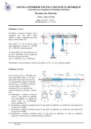
Problema 1 – <strong>Corte</strong> ortogonal<br />
Numa operação <strong>de</strong> corte <strong>por</strong> <strong>arranque</strong> <strong>de</strong> <strong>apara</strong>, que se po<strong>de</strong> representar através <strong>do</strong><br />
mo<strong>de</strong>lo <strong>de</strong> corte ortogonal, utilizou-se uma ferramenta com ângulo <strong>de</strong> saída nulo e<br />
uma velocida<strong>de</strong> da árvore <strong>de</strong> trabalho <strong>de</strong> 350 rpm.<br />
Outros da<strong>do</strong>s:<br />
Diâmetro da peça: 50 mm<br />
Velocida<strong>de</strong> <strong>de</strong> avanço: V A = 120 mm/min<br />
Espessura da <strong>apara</strong>: t c = 1 mm (após o corte)<br />
Largura <strong>de</strong> corte: w = 2mm<br />
Pressão específica <strong>de</strong> corte: k s = 100 Kgf/mm 2 .<br />
Calcular:<br />
a) A potência <strong>de</strong> corte<br />
b) A velocida<strong>de</strong> <strong>de</strong> saída da <strong>apara</strong><br />
c) O ângulo <strong>do</strong> plano <strong>de</strong> escorregamento
Revisão: Geometria <strong>do</strong> corte ortogonal vs. corte oblíquo<br />
z<br />
z<br />
x<br />
χ<br />
χ<br />
x<br />
y<br />
<strong>Corte</strong> Ortogonal (2D)<br />
y<br />
<strong>Corte</strong> Oblíquo (3D)<br />
χ - ângulo <strong>de</strong> posição<br />
No corte ortogonal: χ = 90º
Secção da <strong>apara</strong> – corte oblíquo<br />
b<br />
χ<br />
h<br />
a<br />
p<br />
a – avanço<br />
p – penetração<br />
b – largura da <strong>apara</strong><br />
h – espessura da <strong>apara</strong><br />
χ – ângulo <strong>de</strong> posição<br />
s – secção da <strong>apara</strong><br />
h<br />
=<br />
a<br />
⋅<br />
sin<br />
χ<br />
Secção da <strong>apara</strong>:<br />
b ⋅cos(90º<br />
−χ)<br />
=<br />
p<br />
⇒<br />
b ⋅sin<br />
χ =<br />
p<br />
⇒<br />
b<br />
=<br />
p<br />
sin χ<br />
s<br />
=<br />
b ⋅ h<br />
s<br />
=<br />
p ⋅ a<br />
s<br />
=<br />
b ⋅ a ⋅sin<br />
χ<br />
No corte ortogonal: χ = 90º → h = a
Problema 2 – <strong>Corte</strong> oblíquo<br />
Suponha que dispõe <strong>de</strong> um torno mecânico e que conhece a potência <strong>do</strong> motor com<br />
que está equipa<strong>do</strong>, bem como o rendimento da respectiva ca<strong>de</strong>ia cinemática,<br />
η m = 80%.<br />
Preten<strong>de</strong> maquinar vários varões <strong>de</strong> aço St37, <strong>de</strong>s<strong>de</strong> o diâmetro <strong>de</strong> 50 mm até 40 mm<br />
com uma única passagem, <strong>por</strong> forma a obter o melhor rendimento da máquina<br />
ferramenta.<br />
Outros da<strong>do</strong>s:<br />
Potência <strong>do</strong> motor: N m = 10 Hp<br />
Angulo <strong>de</strong> posição: χ = 45º<br />
Velocida<strong>de</strong> <strong>de</strong> corte aconselhável: V C = 90 mm/min<br />
Pressão específica <strong>de</strong> corte: k s = 170 Kgf/mm 2 .<br />
Calcular:<br />
a) A máxima secção <strong>de</strong> corte da <strong>apara</strong>, sem que o motor entre em sobrecarga<br />
b) A espessura, a largura e o avanço <strong>de</strong> corte<br />
c) O numero <strong>de</strong> rotações <strong>por</strong> minuto da árvore <strong>de</strong> trabalho<br />
d) Se o comprimento da peça for L=1000 mm, quanto tempo levaria a operação <strong>de</strong><br />
maquinagem?
CAD/CAM
CAM no ciclo <strong>de</strong> vida <strong>do</strong> produto
Fresa<strong>do</strong>ra CNC (5 eixos)<br />
5-Axle milling center
Torno CNC<br />
TL-1 DETAILS:<br />
CNC/Manual<br />
406 x 762 mm<br />
max capacity,<br />
406 mm swing,<br />
7.5 hp (5.6 kW)<br />
vector drive,<br />
2000 rpm,<br />
A2-5 spindle,<br />
Intuitive<br />
Programming<br />
System,<br />
1 MB program<br />
memory,<br />
15" color LCD<br />
monitor and USB<br />
<strong>por</strong>t.
Centros <strong>de</strong> maquinagem CNC
Maquinagem CNC<br />
Nos sistemas <strong>de</strong> CNC mo<strong>de</strong>rnos, o<br />
<strong>de</strong>senho <strong>do</strong> componente é efectua<strong>do</strong><br />
através <strong>de</strong> software CAD/CAM<br />
Computer Ai<strong>de</strong>d Design / Computer<br />
Ai<strong>de</strong>d Manufacturing<br />
Os programas CAD/CAM produzem um<br />
ficheiro que é interpreta<strong>do</strong> para dar<br />
origem aos coman<strong>do</strong>s necessários para<br />
operar a máquina através <strong>de</strong> um pós-<br />
processa<strong>do</strong>r a<strong>de</strong>qua<strong>do</strong> e posteriormente<br />
é carrega<strong>do</strong> nas máquinas CNC para<br />
produção <strong>do</strong> componente.<br />
Da<strong>do</strong> que um componente po<strong>de</strong> em geral<br />
requerer a utilização <strong>de</strong> várias<br />
ferramentas, as máquinas mo<strong>de</strong>rnas<br />
combinam normalmente ferramentas<br />
multiplas.
Software CNC<br />
Simulação computacional da<br />
operação <strong>de</strong> maquinagem:<br />
•Definição <strong>do</strong>s percursos da<br />
ferramenta<br />
•Detecção <strong>de</strong> interferências<br />
ferramenta-peça ou ferramentamáquina<br />
•Definição <strong>de</strong> fixações da peça<br />
•Verificação <strong>do</strong>s limites da<br />
máquina
VTT Working Papers 28 – ESPOO<br />
2005, Integration of CAD, CAM and<br />
NC with STEP-NC
STEP-NC<br />
New Mo<strong>de</strong>l for<br />
Data transfer<br />
between<br />
CAD/CAM system<br />
and CNC<br />
machines:<br />
Provi<strong>de</strong>s full<br />
<strong>de</strong>scription of the<br />
part,<br />
manufacturing<br />
process, CAD<br />
<strong>de</strong>sign data,<br />
manufacturing<br />
information,<br />
cutting<br />
characteristics,<br />
tool requirements,<br />
working steps,<br />
etc.<br />
VTT Working Papers 28 – ESPOO<br />
2005, Integration of CAD, CAM and<br />
NC with STEP-NC
Current Manufacturing life cycle<br />
VTT Working Papers 28 – ESPOO<br />
2005, Integration of CAD, CAM and<br />
NC with STEP-NC
STEP-NC<br />
VTT Working Papers 28 – ESPOO<br />
2005, Integration of CAD, CAM and<br />
NC with STEP-NC
![Conceitos transmissao de dados .Sinais[.pdf]](https://img.yumpu.com/50982145/1/190x146/conceitos-transmissao-de-dados-sinaispdf.jpg?quality=85)
![Packages e interfaces[.pdf]](https://img.yumpu.com/50629553/1/190x134/packages-e-interfacespdf.jpg?quality=85)