Sisteme de Ecuatii Diferentiale
Sisteme de Ecuatii Diferentiale
Sisteme de Ecuatii Diferentiale

You also want an ePaper? Increase the reach of your titles
YUMPU automatically turns print PDFs into web optimized ePapers that Google loves.
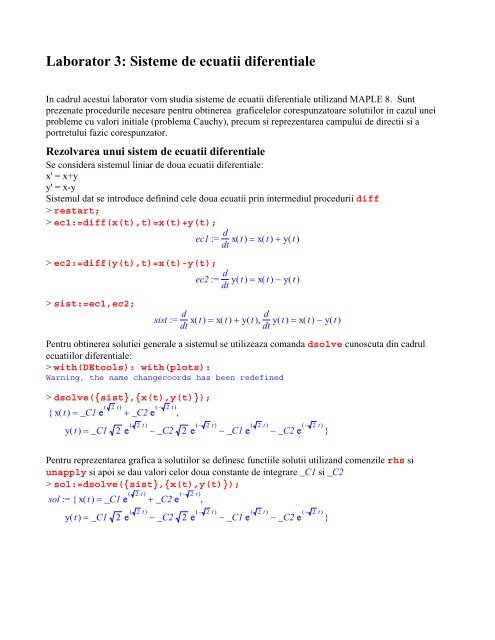
Laborator 3: <strong>Sisteme</strong> <strong>de</strong> ecuatii diferentiale<br />
In cadrul acestui laborator vom studia sisteme <strong>de</strong> ecuatii diferentiale utilizand MAPLE 8. Sunt<br />
prezenate procedurile necesare pentru obtinerea graficelelor corespunzatoare solutiilor in cazul unei<br />
probleme cu valori initiale (problema Cauchy), precum si reprezentarea campului <strong>de</strong> directii si a<br />
portretului fazic corespunzator.<br />
Rezolvarea unui sistem <strong>de</strong> ecuatii diferentiale<br />
Se consi<strong>de</strong>ra sistemul liniar <strong>de</strong> doua ecuatii diferentiale:<br />
x' = x+y<br />
y' = x-y<br />
Sistemul dat se introduce <strong>de</strong>finind cele doua ecuatii prin intermediul procedurii diff<br />
> restart;<br />
> ec1:=diff(x(t),t)=x(t)+y(t);<br />
d<br />
ec1 := x( t ) = x( t ) + y( t )<br />
dt<br />
> ec2:=diff(y(t),t)=x(t)-y(t);<br />
d<br />
ec2 := y( t ) = x( t ) − y( t )<br />
dt<br />
> sist:=ec1,ec2;<br />
d<br />
d<br />
sist := x( t ) = x( t ) + y( t ) , y( t ) = x( t ) − y( t )<br />
dt<br />
dt<br />
Pentru obtinerea solutiei generale a sistemul se utilizeaza comanda dsolve cunoscuta din cadrul<br />
ecuatiilor diferentiale:<br />
> with(DEtools): with(plots):<br />
Warning, the name changecoords has been re<strong>de</strong>fined<br />
> dsolve({sist},{x(t),y(t)});<br />
( 2 t)<br />
( − 2 t)<br />
{ x( t ) = _C1 e + _C2 e ,<br />
( 2 t)<br />
( − 2 t)<br />
( 2 t)<br />
y( t ) = _C1 2 e − _C2 2 e − _C1 e − _C2 e<br />
( − 2 t)<br />
}<br />
Pentru reprezentarea grafica a solutiilor se <strong>de</strong>finesc functiile solutii utilizand comenzile rhs si<br />
unapply si apoi se dau valori celor doua constante <strong>de</strong> integrare _C1 si _C2<br />
> sol:=dsolve({sist},{x(t),y(t)});<br />
( 2 t)<br />
( − 2 t)<br />
sol := { x( t ) = _C1 e + _C2 e ,<br />
( 2 t)<br />
( − 2 t)<br />
( 2 t)<br />
y( t ) = _C1 2 e − _C2 2 e − _C1 e − _C2 e<br />
( )<br />
− 2 t<br />
}
Atentie variabila sol este o lista, accesul la x(t) si y(t) se face prin sol[1], respectiv sol[2]<br />
> xx:=unapply(rhs(sol[1]),t,_C1,_C2);<br />
( 2 t)<br />
xx := ( t, _C1, _C2 ) → _C1 e + _C2 e<br />
> yy:=unapply(rhs(sol[2]),t,_C1,_C2);<br />
( 2 t)<br />
( − 2 t)<br />
( 2 t)<br />
( − 2 t)<br />
yy := ( t, _C1, _C2 ) → _C1 2 e − _C2 2 e − _C1 e − _C2 e<br />
( − 2 t)<br />
In variabilele xx si yy avem expresiile solutiilor sub forma unor functii ce <strong>de</strong>pind <strong>de</strong> variabila<br />
in<strong>de</strong>pen<strong>de</strong>nta si cele doua constante <strong>de</strong> integrare. Daca dorim sa obtinem graficele solutiilor pentru<br />
constantele _C1=1 si _C2=1 se utilizeaza comanda plot<br />
> plot(xx(t,1,1),t=-4..4);<br />
> plot(yy(t,1,1),t=-4..4);
sau pot fi reprezentate ambele solutii in acelasi grafic:<br />
> plot([xx(t,1,1),yy(t,1,1)],t=-4..4,color=[red,blue]);<br />
Probleme Cauchy<br />
Daca dorim obtinerea solutiilor corespunzatoare unei probleme cu valori initiale, <strong>de</strong> exemplu:<br />
x' = x+y<br />
y' = x-y<br />
x(0) = 1<br />
y(0) = 0<br />
se <strong>de</strong>finesc conditiile initiale ca in cazul ecuatiilor diferentiale:<br />
> cond_in:=x(0)=1, y(0)=0;<br />
cond_in := x0 ( ) = 1 , y0 ( ) = 0<br />
iar pentru obtinerea solutiilor se utilizeaza, din nou, comanda dsolve precizandu-se conditiile initiale:<br />
> sol:=dsolve({sist,cond_in},{x(t),y(t)});<br />
⎛1<br />
sol x( t ) =<br />
⎝<br />
⎜ +<br />
2<br />
2 ⎞ (<br />
4 ⎠<br />
⎟ e<br />
)<br />
+<br />
2 t := {<br />
⎛1<br />
⎝<br />
⎜ −<br />
2<br />
2 ⎞ ( − 2 t)<br />
4 ⎠<br />
⎟ e , y( t ) =<br />
⎛1<br />
⎝<br />
⎜ +<br />
2<br />
2 ⎞<br />
4 ⎠<br />
⎟<br />
(<br />
2 e<br />
)<br />
− − −<br />
2 t ⎛1<br />
⎝<br />
⎜ −<br />
2<br />
2 ⎞<br />
4 ⎠<br />
⎟<br />
( )<br />
2 e − 2 t ⎛1<br />
⎝<br />
⎜ +<br />
2<br />
2 ⎞ (<br />
4 ⎠<br />
⎟ e<br />
) 2 t ⎛1<br />
⎝<br />
⎜ −<br />
2<br />
2 ⎞ ( − 2 t)<br />
4 ⎠<br />
⎟ e }<br />
Pentru reprezentarea grafica a solutiilor avem doua alternative. Prima varianta este sa <strong>de</strong>finim functiile<br />
solutii utilizand comenzile rhs si unapply (ca in cazul solutiei generale):<br />
> xx:=unapply(rhs(sol[1]),t);<br />
⎛1<br />
xx := t →<br />
⎝<br />
⎜ +<br />
2<br />
2 ⎞ (<br />
4 ⎠<br />
⎟ e<br />
)<br />
+<br />
2 t ⎛1<br />
⎝<br />
⎜ −<br />
2<br />
> yy:=unapply(rhs(sol[2]),t);<br />
yy := t →<br />
⎛1<br />
⎝<br />
⎜ +<br />
2<br />
2<br />
4<br />
⎞<br />
⎠<br />
⎟<br />
2<br />
4<br />
⎞<br />
⎠<br />
⎟<br />
e<br />
( − 2 t)<br />
( )<br />
2 e − − −<br />
2 t ⎛1<br />
2 ⎞ ( )<br />
⎝<br />
⎜ −<br />
2 4 ⎠<br />
⎟ 2 e − 2 t ⎛1<br />
2 ⎞ ( )<br />
⎝<br />
⎜ +<br />
2 4 ⎠<br />
⎟ e 2 t ⎛1<br />
⎝<br />
⎜ −<br />
2<br />
2<br />
4<br />
⎞<br />
⎠<br />
⎟<br />
e<br />
( − 2 t)
si apoi utilizam comanda plot<br />
> plot(xx(t),t=-5..5);<br />
> plot(yy(t),t=-5..5);<br />
sau pot fi reprezentate ambele solutii in acelasi grafic:<br />
> plot([xx(t),yy(t)],t=-5..5,color=[red,blue]);
A doua varianta <strong>de</strong> reprezentare grafica a solutiilor este utlizarea comenzii DEplot cu optiunea<br />
scene<br />
> DEplot([sist],[x,y],t=5..5,[[cond_in]],linecolor=blue,<br />
scene=[t,x(t)]);<br />
> DEplot([sist],[x,y],t=-5..5,[[cond_in]], linecolor=red,<br />
scene=[t,y(t)]);<br />
In cazul in care dorim reprezentarea grafica a ambelor solutii in acelasi grafic utilizand comanda<br />
DEplot vom utiliza intructiunile:<br />
> xx1:=DEplot([sist],[x,y],t=-5..5,[[cond_in]], linecolor=blue,<br />
scene=[t,x(t)]):<br />
> yy1:=DEplot([sist],[x,y],t=-5..5,[[cond_in]],linecolor=red,<br />
scene=[t,y(t)]):<br />
> display([xx1,yy1]);
Campul <strong>de</strong> directii. Portret Fazic<br />
Pentru reprezentarea campului <strong>de</strong> directii utilizam instructiunea:<br />
> DEplot([sist],[x(t),y(t)],t=-4..4,x=-10..10,y=-10..10,<br />
arrows=medium);<br />
iar pentru reprezentarea portretului fazic (campul <strong>de</strong> directii si cateva orbite) vom utiliza aceeasi<br />
instructiune cu diferenta ca sunt precizate anumite conditii initiale reprezentand curbele ce trec prin<br />
punctele precizate:<br />
> DEplot([sist],[x(t),y(t)],t=-4..4,x=-10..10,y=-10..10,<br />
[[x(0)=1,y(0)=0], [x(0)=1,y(0)=5]], arrows=medium, linecolor=blue);
In acest grafic avem reprezentate doua orbite, daca dorim reprezentarea mai multor orbite trebuiesc<br />
precizate mai multe conditii initiale:<br />
> cond_in2:=[x(0)=0,y(0)=i]$i=1..5, [x(0)=0,y(0)=-i]$i=1..5,<br />
[x(0)=i,y(0)=0]$i=1..5, [x(0)=-i,y(0)=0]$i=1..5;<br />
cond_in2 := [ x0 ( ) = 0 , y0 ( ) = 1 ] , [ x0 ( ) = 0 , y0 ( ) = 2 ] , [ x0 ( ) = 0 , y0 ( ) = 3]<br />
,<br />
[ x0 ( ) = 0 , y0 ( ) = 4 ] , [ x0 ( ) = 0 , y0 ( ) = 5 ] , [ x0 ( ) = 0 , y0 ( ) = -1]<br />
,<br />
[ x0 ( ) = 0 , y0 ( ) = -2 ] , [ x0 ( ) = 0 , y0 ( ) = -3 ] , [ x0 ( ) = 0 , y0 ( ) = -4]<br />
,<br />
[ x0 ( ) = 0 , y0 ( ) = -5 ] , [ x0 ( ) = 1 , y0 ( ) = 0 ] , [ x0 ( ) = 2 , y0 ( ) = 0]<br />
,<br />
[ x0 ( ) = 3 , y0 ( ) = 0 ] , [ x0 ( ) = 4 , y0 ( ) = 0 ] , [ x0 ( ) = 5 , y0 ( ) = 0]<br />
,<br />
[ x0 ( ) = -1 , y0 ( ) = 0 ] , [ x0 ( ) = -2,<br />
y0 ( ) = 0 ] , [ x0 ( ) = -3 , y0 ( ) = 0]<br />
,<br />
[ x0 ( ) = -4 , y0 ( ) = 0 ] , [ x0 ( ) = -5 , y0 ( ) = 0]<br />
> DEplot([sist],[x(t),y(t)],t=-5..5,x=-10..10,y=-10..10,[cond_in2],<br />
arrows=medium, linecolor=blue,stepsize=0.1);