A Framework for Evaluating Early-Stage Human - of Marcus Hutter

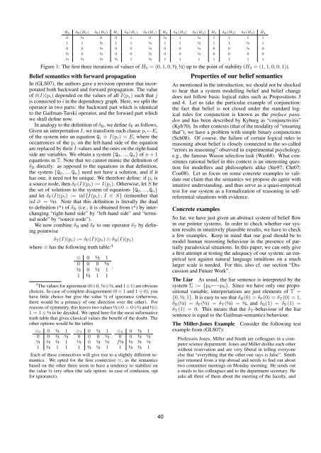
H0 δB(H0) δF(H0) H1 δB(H1) δF(H1) H2 δB(H2) δF(H2) H3 δB(H3) δF(H3) H4
0 ½ 0 0 1 0 ½ 1 ½ 1 1 1 1
1 1 ½ 1 1 ½ 1 1 ½ 1 1 ½ 1
0 0 ½ 0 0 ½ 0 0 ½ 0 0 ½ 0
½ 0 ½ 0 0 ½ 0 0 ½ 0 0 0 0
½ ½ ½ ½ 1 ½ 1 1 1 1 1 1 1
Figure 1: The first three iterations of values of H0 = (0, 1, 0, ½, ½) up to the point of stability (H3 = (1, 1, 0, 0, 1)).
Belief semantics with forward propagation
In (GLS07), the authors gave a revision operator that incorporated
both backward and forward propagation. The value
of δ(I)(pi) depended on the values of all I(pj) such that j
is connected to i in the dependency graph. Here, we split the
operator in two parts: the backward part which is identical
to the Gaifman-Tarski operator, and the forward part which
we shall define now.
In analogy to the definition of δB, we define δF as follows.
Given an interpretation I, we transform each clause pi←Ei
of the system into an equation Qi ≡ I(pi) = Ei where the
occurrences of the pi on the left-hand side of the equation
are replaced by their I-values and the ones on the right-hand
side are variables. We obtain a system {Q0, ..., Qn} of n + 1
equations in T. Note that we cannot mimic the definition of
δB directly: as opposed to the equations in that definition,
the system {Q0, ..., Qn} need not have a solution, and if it
has one, it need not be unique. We therefore define: if pi is
a source node, then δF(I)(pi) := I(pi). Otherwise, let S be
the set of solutions to the system of equations {Q0, ..., Qn}
and let δF(I)(pi) := inf{I(pi) ; I ∈ S} (remember that
inf ∅ = ½). Note that this definition is literally the dual
to definition (*) of δB (i.e., it is obtained from (*) by interchanging
“right-hand side” by “left-hand side” and “terminal
node” by “source node”).
We now combine δB and δF to one operator δT by defining
pointwise
δT(I)(pi) := δF(I)(pi) ⊗ δB(I)(pi)
where ⊗ has the following truth table: 4
⊗ 0 ½ 1
0 0 0 ½
½ 0 ½ 1
1 ½ 1 1
4 The values for agreement (0⊗0, ½⊗½, and 1⊗1) are obvious
choices. In case of complete disagreement (0 ⊗ 1 and 1 ⊗ 0), you
have little choice but give the value ½ of ignorance (otherwise,
there would be a primacy of one direction over the other). For
reasons of symmetry, this leaves two values ½⊗0 = 0⊗½ and ½⊗
1 = 1 ⊗ ½ to be decided. We opted here for the most informative
truth table that gives classical values the benefit of the doubt. The
other options would be the tables
⊗0 0 ½ 1
0 0 ½ ½
½ ½ ½ 1
1 ½ 1 1
⊗1 0 ½ 1
0 0 0 ½
½ 0 ½ ½
1 ½ ½ 1
.
⊗2 0 ½ 1
0 0 ½ ½
f½ ½ ½ ½
1 ½ ½ 1
Each of these connectives will give rise to a slightly different semantics.
We opted for the first connective ⊗, as the semantics
based on the other three seem to have a tendency to stabilize on
the value ½ very often (the safe option: in case of confusion, opt
for ignorance).
.
40
Properties of our belief semantics
As mentioned in the introduction, we should not be shocked
to hear that a system modelling belief and belief change
does not follow basic logical rules such as Propositions 3
and 4. Let us take the particular example of conjunction:
the fact that belief is not closed under the standard logical
rules for conjunction is known as the preface paradox
and has been described by Kyburg as “conjunctivitis”
(Kyb70). In other contexts (that of the modality of “ensuring
that”), we have a problem with simple binary conjunctions
(Sch08). Of course, the failure of certain logical rules in
reasoning about belief is closely connected to the so-called
“errors in reasoning” observed in experimental psychology,
e.g., the famous Wason selection task (Was68). What constitutes
rational belief in this context is an interesting question
for modellers and philosophers alike (Ste97; Chr07;
Cou08). Let us focus on some concrete examples to validate
our claim that the semantics we propose do agree with
intuitive understanding, and thus serve as a quasi-empirical
test for our system as a formalization of reasoning in selfreferential
situations with evidence.
Concrete examples
So far, we have just given an abstract system of belief flow
in our pointer systems. In order to check whether our system
results in intuitively plausible results, we have to check
a few examples. Keep in mind that our goal should be to
model human reasoning behaviour in the presence of partially
paradoxical situations. In this paper, we can only give
a first attempt at testing the adequacy of our system: an empirical
test against natural language intuitions on a much
larger scale is needed. For this, also cf. our section “Discussion
and Future Work”.
The Liar As usual, the liar sentence is interpreted by the
system Σ := {p0←¬p0}. Since we have only one propositional
variable, interpretations are just elements of T =
{0, ½, 1}. It is easy to see that δB(0) = δF(0) = δT(0) = 1,
δB(½) = δF(½) = δT(½) = ½, and δB(1) = δF(1) =
δT(1) = 0. This means that the δT-behaviour of the liar
sentence is equal to the Gaifman-semantics behaviour.
The Miller-Jones Example Consider the following test
example from (GLS07):
Professors Jones, Miller and Smith are colleagues in a computer
science department. Jones and Miller dislike each other
without reservation and are very liberal in telling everyone
else that “everything that the other one says is false”. Smith
just returned from a trip abroad and needs to find out about
two committee meetings on Monday morning. He sends out
e-mails to his colleagues and to the department secretary. He
asks all three of them about the meeting of the faculty, and