A Framework for Evaluating Early-Stage Human - of Marcus Hutter

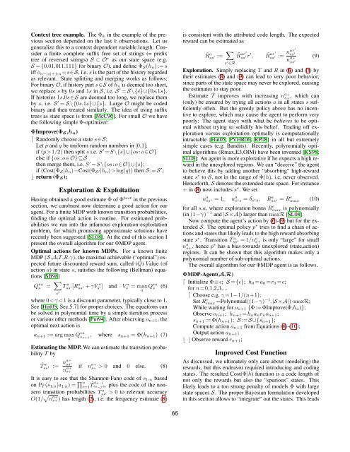
Context tree example. The Φk in the example of the previous
section depended on the last k observations. Let us
generalize this to a context dependent variable length: Consider
a finite complete suffix free set of strings (= prefix
tree of reversed strings) S ⊂ O ∗ as our state space (e.g.
S = {0,01,011,111} for binary O), and define ΦS(hn) := s
iff o n−|s|+1:n =s∈S, i.e. s is the part of the history regarded
as relevant. State splitting and merging works as follows:
For binary O, if history part s∈S of hn is deemed too short,
we replace s by 0s and 1s in S, i.e. S ′ = S \{s}∪{0s,1s}.
If histories 1s,0s ∈ S are deemed too long, we replace them
by s, i.e. S ′ = S \{0s,1s}∪{s}. Large O might be coded
binary and then treated similarly. The idea of using suffix
trees as state space is from [McC96]. For small O we have
the following simple Φ-optimizer:
ΦImprove(ΦS,hn)
⌈ Randomly choose a state s∈S;
Let p and q be uniform random numbers in [0,1];
if (p>1/2) then split s i.e. S ′ =S\{s}∪{os:o∈O}
else if {os:o∈O}⊆S
then merge them, i.e. S ′ =S\{os:o∈O}∪{s};
if (Cost(ΦS|hn)−Cost(ΦS ′|hn)>log(q)) then S :=S ′ ;
⌊ return (ΦS);
Exploration & Exploitation
Having obtained a good estimate ˆ Φ of Φbest in the previous
section, we can/must now determine a good action for our
agent. For a finite MDP with known transition probabilities,
finding the optimal action is routine. For estimated probabilities
we run into the infamous exploration-exploitation
problem, for which promising approximate solutions have
recently been suggested [SL08]. At the end of this section I
present the overall algorithm for our ΦMDP agent.
Optimal actions for known MDPs. For a known finite
MDP (S,A,T,R,γ), the maximal achievable (“optimal”) expected
future discounted reward sum, called (Q) Value (of
action a) in state s, satisfies the following (Bellman) equations
[SB98]
Q ∗a
s = �
T a ss ′[Ra ∗
∗
ss ′ + γVs ′] and Vs = max s (6)
s ′
a Q∗a
where 0 0 to relevant accuracy
O(1/ � n a+
s+) has length (2), i.e. the frequency estimate (8)
65
is consistent with the attributed code length. The expected
reward can be estimated as
ˆR a �
ss ′ :=
r ′ ˆR
∈R
ar′
ss ′ r′ ,
Rˆ ar ′ nar′ ss
ss ′ := ′
n a+
ss ′
Exploration. Simply replacing T and R in (6) and (7) by
their estimates (8) and (9) can lead to very poor behavior,
since parts of the state space may never be explored, causing
the estimates to stay poor.
Estimate ˆ T improves with increasing na+ s+, which can
(only) be ensured by trying all actions a in all states s sufficiently
often. But the greedy policy above has no incentive
to explore, which may cause the agent to perform very
poorly: The agent stays with what he believes to be optimal
without trying to solidify his belief. Trading off exploration
versus exploitation optimally is computationally
intractable [Hut05; PVHR06; RP08] in all but extremely
simple cases (e.g. Bandits). Recently, polynomially optimal
algorithms (Rmax,E3,OIM) have been invented [KS98;
SL08]: An agent is more explorative if he expects a high reward
in the unexplored regions. We can “deceive” the agent
to believe this by adding another “absorbing” high-reward
state se to S, not in the range of Φ(h), i.e. never observed.
Henceforth, S denotes the extended state space. For instance
+ in (8) now includes se . We set
(9)
n a ss e = 1, na s e s = δs e s, R a ss e = Re max (10)
for all s,a, where exploration bonus R e max is polynomially
(in (1−γ) −1 and |S ×A|) larger than maxR [SL08].
Now compute the agent’s action by (6)-(9) but for the extended
S. The optimal policy p ∗ tries to find a chain of actions
and states that likely leads to the high reward absorbing
state s e . Transition ˆ T a ss e = 1/na s+ is only “large” for small
n a s+, hence p ∗ has a bias towards unexplored (state,action)
regions. It can be shown that this algorithm makes only a
polynomial number of sub-optimal actions.
The overall algorithm for our ΦMDP agent is as follows.
ΦMDP-Agent(A,R)
⌈ Initialize Φ≡ɛ; S ={ɛ}; h0 =a0 =r0 =ɛ;
for n=0,1,2,3,...
⌈ Choose e.g. γ =1−1/(n+1);
Set R e max =Polynomial((1−γ) −1 ,|S ×A|)·maxR;
While waiting for on+1 {Φ:=ΦImprove(Φ,hn)};
Observe on+1; hn+1 =hnanrnon+1;
sn+1 :=Φ(hn+1); S :=S ∪{sn+1};
Compute action an+1 from Equations (6)-(10);
Output action an+1;
⌊ ⌊ Observe reward rn+1;
Improved Cost Function
As discussed, we ultimately only care about (modeling) the
rewards, but this endeavor required introducing and coding
states. The resulted Cost(Φ|h) function is a code length of
not only the rewards but also the “spurious” states. This
likely leads to a too strong penalty of models Φ with large
state spaces S. The proper Bayesian formulation developed
in this section allows to “integrate” out the states. This leads