ACME 2011 Proceedings of the 19 UK National Conference of the ...

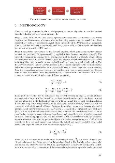
Figure 1: Proposed methodology for arterial elasticity estimation.
2 METHODOLOGY
The methodology employed for the arterial property estimation algorithm is broadly classified
into the following stages as shown in figure 1.
Stage 0 deals with the real-time patient specific data acquisition via dynamic MRI, which
captures the displacement of arteries due to distending pressure as the blood flows. Data
acquired here acts as a benchmark against which the results of the CFD model are compared.
This stage is not included in the current work but is essential in establishing the link between
the human body and the CFD model.
Stage 1 constitutes the solution for the forward problem, which employs an explicit scheme
to solve the governing 1D equations (1),(2) applied to flow through compliant tubes [3]. The
arterial deformation in response to the cardiac output of the heart is artificially obtained from
the blood-flow model in terms of the nodal area. The solution procedure also results in the nodal
velocity of blood and the nodal pressure is finally evaluated using area and velocity values. The
Locally Conservative Taylor-Galerkin method (LCG) that is employed in the solution scheme
helps reduce computational effort as it prevents the need to invert huge matrices originating
from the conventional assembly process, by treating each element as a separate sub-domain
with its own boundaries. Also, the incorporation of discontinuities is simplified in LCG as
co-located nodes are permitted to have different properties.
∂u
∂t
∂A
∂t
+ u∂u
∂x
+ ∂(Au)
∂x
= 0 (1)
1 ∂p 1 ∂τ
+ + = 0 (2)
ρ ∂x ρ ∂x
It should be noted that for the solution of the forward problem in stage 1, arterial stiffness
was assumed to be known, but in real life problems the stiffness is actually not known a priori
and its estimation is the hallmark of this work. Even though the forward problem solution
is obtained only after using stiffness as an user input, inverse property estimation can be
employed to yield the actual stiffness of arteries by making comparisons between the model
predicted and experimental data. The Levenberg Marquardt (LM) optimization is used here
[4, 5]. It is an iterative technique that locates a local minimum of a multivariate function that is
expressed as the sum of squares of several non-linear, real-valued functions. It has been adopted
in various data-fitting applications and has become a standard technique for non-linear least
squares problems. As a starting point, an objective function incorporating just nodal areas is
considered. It is the least square error between the actual and model predicted area (nodal
basis). The objective function is as expressed in equation (3).
n�
2
f = (Aj − Aj)
j=1
where, Aj is a vector of actual nodal areas (experimental data), Aj is a vector of model predicted
nodal areas and j corresponds to the number of nodes. The LM algorithm operates by
minimizing this objective function which in a physical sense is equivalent to repeating the forward
run in an intelligent manner until the measured displacements equal the model predicted
(3)
18