Lake Brownwood Watershed - Texas State Soil and Water ...
Lake Brownwood Watershed - Texas State Soil and Water ...
Lake Brownwood Watershed - Texas State Soil and Water ...

You also want an ePaper? Increase the reach of your titles
YUMPU automatically turns print PDFs into web optimized ePapers that Google loves.
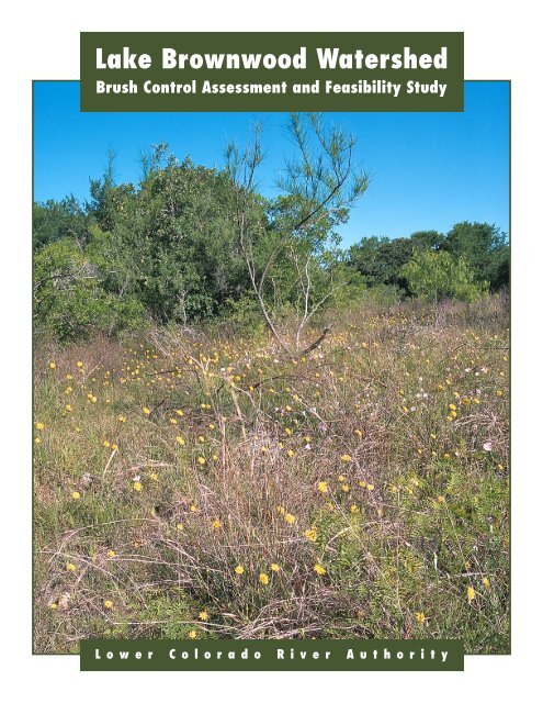
<strong>Lake</strong> <strong>Brownwood</strong> <strong><strong>Water</strong>shed</strong><br />
Brush Control Assessment <strong>and</strong> Feasibility Study<br />
Lower Colorado River Authority
ABOUT LCRA<br />
LCRA is a conservation <strong>and</strong> reclamation district created by the <strong>Texas</strong> Legislature in<br />
1934 to provide energy, water <strong>and</strong> community services to the people of <strong>Texas</strong>.<br />
LCRA cannot levy taxes, but gets its income to fund its operations from the sale of<br />
electricity, water <strong>and</strong> other services.<br />
LCRA sells wholesale electricity to city-owned utilities <strong>and</strong> cooperatives that serve<br />
more than 1 million people in <strong>Texas</strong>. LCRA also sells stored water; develops <strong>and</strong><br />
operates water <strong>and</strong> wastewater utilities; manages the lower Colorado River;<br />
protects water quality; owns <strong>and</strong> operates parks; promotes conservation of soil,<br />
water <strong>and</strong> energy; <strong>and</strong> offers economic <strong>and</strong> community development assistance to<br />
rural communities.<br />
LOWER COLORADO RIVER AUTHORITY<br />
P.O. Box 220<br />
Austin, <strong>Texas</strong> 78767-0220<br />
1-800-776-5272<br />
(512) 473-3200<br />
www.lcra.org<br />
Printed on recycled paper with soy-based ink.<br />
NOVEMBER 2002
LAKE BROWNWOOD WATERSHED<br />
Brush Control Assessment <strong>and</strong> Feasibility Study<br />
Lower Colorado River Authority<br />
Copyright 2002
TABLE OF CONTENTS<br />
Section Page<br />
TABLE OF CONTENTS ii<br />
LIST OF FIGURES iii<br />
ACKNOWLEDGEMENTS iv<br />
1.0 INTRODUCTION 1-1<br />
2.0 EXECUTIVE SUMMARY 2-1<br />
3.0 HYDROLOGIC EVALUATION 3-1<br />
3.1 DESCRIPTION OF THE WATERSHED 3-1<br />
3.2 HISTORICAL CONSIDERATIONS 3-6<br />
3.2.1 VEGETATION HISTORY 3-6<br />
3.2.2 HYDROLOGICAL HISTORY 3-12<br />
3.3 GEOLOGICAL CONSIDERATIONS 3-14<br />
3.4 EXISTING SURFACE WATER HYDROLOGY 3-16<br />
3.5 EXISTING GROUNDWATER HYDROLOGY 3-16<br />
3.6 DESCRIPTION OF THE WATERSHED HYDROLOGIC SYSTEM 3-17<br />
3.7 SUMMARY AND CONCLUSIONS 3-17<br />
4.0 REFERENCES 4-1<br />
APPENDIX 1 A1-1<br />
APPENDIX 2 A2-1<br />
APPENDIX 3 A3-1<br />
APPENDIX 4 A4-1<br />
ii
LIST OF FIGURES<br />
Figure Page<br />
3-1 General Brush Control Zone 3-2<br />
3-2 Study Area Location 3-4<br />
3-3 Natural Regions <strong>and</strong> Subregions of <strong>Texas</strong> 3-5<br />
3-4 General Vegetation Mapping of Study Area 3-10<br />
3-5 2000 <strong><strong>Water</strong>shed</strong> Vegetation Map 3-11<br />
3-6 Geologic Map of the Study Area 3-15<br />
iii
ACKNOWLEDGEMENTS<br />
This report is the result of a collaborative effort between the Lower Colorado River Authority, the <strong>Texas</strong> <strong>State</strong> <strong>Soil</strong><br />
<strong>and</strong> <strong>Water</strong> Conservation Board (TSSWCB), the Coleman County <strong>Soil</strong> & <strong>Water</strong> Conservation District (SWCD), the Pecan<br />
Bayou SWCD, the U. S. Department of Agriculture’s Natural Resources Conservation Service (NRCS), <strong>and</strong> the <strong>Texas</strong><br />
A&M University System (TAMU). Professionals from each of these entities provided valuable input, which, in turn,<br />
resulted in the creation of a document that reflects the views of various interests from local l<strong>and</strong>owners to government<br />
agencies. A debt of gratitude goes out to all who gave their time <strong>and</strong> effort.<br />
Special thanks is given to those who played a primary role in the preparation of this report. They include:<br />
Lin Poor Rusty Ray Nadira Kabir<br />
Rich Winkelbauer Jobaid Kabir Stan Casey<br />
Kevin Wagner Steven Bednarz Tim Dybala<br />
Carl Amonett Johnny Jamison Bruce Pittard<br />
Jerry Allen Harold Phillips Joe Ed Wise<br />
Jule W. Richmond Bobby J. Clark Delbert Connaway<br />
O. B. Byrd Jerry Winfrey Sam Oswood<br />
iv
1.0 INTRODUCTION<br />
In 1985, the <strong>Texas</strong> Legislature established a brush control program for the state. As defined in the enabling<br />
legislation, brush control means selective control, removal or reduction of noxious brush such as mesquite, prickly pear,<br />
salt cedar or other deep-rooted plants that consume large amounts of water. The <strong>Texas</strong> <strong>State</strong> <strong>Soil</strong> <strong>and</strong> <strong>Water</strong> Conservation<br />
Board (TSSWCB) was given jurisdiction of the program <strong>and</strong> was directed to prepare <strong>and</strong> adopt a brush control plan that<br />
includes a strategy for managing brush in areas where brush is contributing to a substantial water conservation problem. In<br />
addition, the plan is to designate areas of critical need in which to implement brush control programs. In designating critical<br />
areas under the plan, TSSWCB is required to consider:<br />
the locations of brush infestations;<br />
the type <strong>and</strong> severity of brush infestations;<br />
the management methods that may be used to control brush; <strong>and</strong><br />
any other criteria that the Board considers relevant to ensure that the brush control program can be most<br />
effectively, efficiently <strong>and</strong> economically implemented.<br />
In designating critical areas, the TSSWCB shall give priority to areas with the most critical water conservation<br />
needs <strong>and</strong> those in which brush control <strong>and</strong> revegetation projects will be most likely to produce a substantial increase in the<br />
amount of available <strong>and</strong> usable water.<br />
In 2001, the <strong>Texas</strong> Legislature provided appropriations through the TSSWCB for feasibility studies for four<br />
watersheds on the effects of brush management on water yields. The studies will focus on the changing water yields<br />
associated with brush management <strong>and</strong> the related economic aspects. The <strong>Lake</strong> <strong>Brownwood</strong> watershed is one of the four<br />
watersheds that was funded for study.<br />
The overall goal of this project is to increase the streamflow <strong>and</strong> water availability of Pecan Bayou <strong>and</strong> Jim Ned<br />
Creek into <strong>Lake</strong> <strong>Brownwood</strong> <strong>and</strong> other reservoirs in the watershed for use as a supply of industrial, agricultural, municipal<br />
<strong>and</strong> other water use. The first stage of the project is the goal of this report; to plan <strong>and</strong> assess the feasibility of brush<br />
management to meet the project’s goals. The objectives of this study are to:<br />
develop a historical profile of the vegetation in the <strong>Lake</strong> <strong>Brownwood</strong> watershed.<br />
develop a hydrological profile of the <strong>Lake</strong> <strong>Brownwood</strong> <strong><strong>Water</strong>shed</strong>.<br />
evaluate climatic data throughout the past century <strong>and</strong> its relative effects on the current hydrological<br />
conditions in the <strong>Lake</strong> <strong>Brownwood</strong> watershed.<br />
The Lower Colorado River Authority (LCRA) was contracted by the TSSWCB to investigate <strong>and</strong> produce the<br />
following portion of this report on the <strong>Lake</strong> <strong>Brownwood</strong> watershed:<br />
the watershed’s location, climate, geology, soils, current water use <strong>and</strong> projected water needs.<br />
the current <strong>and</strong> historical l<strong>and</strong>use/l<strong>and</strong> cover (brush type, density <strong>and</strong> canopy cover) <strong>and</strong> observable trends.<br />
the current <strong>and</strong> historical surface <strong>and</strong> groundwater hydrology <strong>and</strong> observable trends.<br />
the potential impacts of a brush control program on wildlife, especially endangered species, are also addressed.<br />
The overall study has been a cooperative ecosystem-level approach that involved LCRA, the TSSWCB, Coleman<br />
<strong>Soil</strong> <strong>and</strong> <strong>Water</strong> Conservation District (SWCD), Pecan Bayou SWCD, NRCS, <strong>and</strong> <strong>Texas</strong> A&M University (TAMU). The<br />
reports produced by the NRCS <strong>and</strong> TAMU are included in this document as Appendices 1-4.<br />
1-1
2.0 EXECUTIVE SUMMARY<br />
As <strong>Texas</strong> seeks to secure additional water supplies to sustain it in the 21st century, policy makers will consider a<br />
variety of options including brush control to meet future water needs. Where it is environmentally <strong>and</strong> ecologically sound,<br />
replacing brush with grasses that use less water could supply <strong>Texas</strong> with additional amounts of relatively inexpensive<br />
water. The goal of this study was to evaluate the climate, vegetation, soil, topography, geology, <strong>and</strong> hydrology of the <strong>Lake</strong><br />
<strong>Brownwood</strong> River watershed with regard to the feasibility of implementing brush control programs in the watershed.<br />
Based on historical evidence <strong>and</strong> more recent regional descriptions, it is apparent that the vegetational l<strong>and</strong>scape of<br />
the <strong>Lake</strong> <strong>Brownwood</strong> watershed has changed considerably over the past 150 years. The early European settlers who<br />
migrated to the area by the mid to late 1800s found a vast expanse of midgrass to tallgrass prairies typical of the Rolling<br />
Plains. Distinct l<strong>and</strong> use changes brought on by settlement <strong>and</strong> an extensive drought precipitated a widespread<br />
transformation of the l<strong>and</strong>scape by the end of the nineteenth century. This change included a great increase in the amount<br />
<strong>and</strong> distribution of woody species, particularly honey mesquite (Prosopis gl<strong>and</strong>ulosa). The once distinct boundaries among<br />
the various habitat types have become blurred, as each community assemblage has become more homogenous <strong>and</strong><br />
grassl<strong>and</strong>s have almost disappeared.<br />
Meteorological data collected in the vicinity of the <strong>Lake</strong> <strong>Brownwood</strong> watershed since the late 1800s indicate that<br />
climatic conditions have not changed significantly over the past century. The exception is reduced precipitation during the<br />
record drought from 1946 to 1957. The average annual temperature in the watershed is approximately 64.4° F, <strong>and</strong> the<br />
average annual rainfall is approximately 25.9 inches. Segments of Pecan Bayou, Jim Ned Creek <strong>and</strong> Hords Creek were<br />
gauged at various times between 1923 <strong>and</strong> 1990, but the periods of record for the gauges are different, <strong>and</strong> nearly all of the<br />
gauges are located downstream of surface reservoirs with controlled release.<br />
There is no evidence to suggest that groundwater levels have declined systematically in the aquifers beneath the<br />
watershed within the evaluation period. A decrease in water levels would be expected if aquifer recharge had declined due<br />
to increased evapotranspiration caused by brush infestation. Observed changes in water levels in watershed aquifers are<br />
more likely due to variations in natural rainfall <strong>and</strong> groundwater withdrawals.<br />
Although the hydrologic data available for this study were not adequate for determining if water yields in the <strong>Lake</strong><br />
<strong>Brownwood</strong> watershed have been affected by brush infestation, geologic <strong>and</strong> hydrologic conditions in the watershed are<br />
very conducive to enhancement of water yields through brush management. Analysis found in Appendices 1-4 are based<br />
on the period of 1960-1999. Further evaluations that include the drought of record may prove to be useful in predicting<br />
water availability for future water supplies.<br />
Current <strong>and</strong> projected water dem<strong>and</strong>s in the watershed are expected to result in water shortages in the future,<br />
especially in the rural areas of Brown County that depend heavily on groundwater resources. In addition, larger water<br />
supply shortages are projected to occur in the lower Colorado River basin downstream of <strong>Lake</strong> <strong>Brownwood</strong>. Brush<br />
management may be an effective means of improving surface water <strong>and</strong> groundwater supplies in the watershed. However,<br />
it should be noted that modeling of such scenarios is dependent on input variables that are subject to interpretation..<br />
2-1
3.0 HYDROLOGIC EVALUATION<br />
The following water balance equation can be used to estimate water yield (i.e., runoff <strong>and</strong> deep drainage) in a<br />
watershed:<br />
Runoff + Deep Drainage = Precipitation – Evapotranspiration.<br />
Runoff = water exiting the watershed via overl<strong>and</strong> flow.<br />
Deep drainage = water exiting the watershed via soil percolation below the plant root zone.<br />
Precipitation = water that falls in the watershed as rain or snow.<br />
Evapotranspiration = water returned to the atmosphere through the processes of evaporation <strong>and</strong> transpiration.<br />
Evaporation is the process by which surface water, water in soil, <strong>and</strong> water adhered to plants returns to the atmosphere as<br />
water vapor. Transpiration is the process by which water vapor passes through plant tissue<br />
The above relationship suggests water yield can be increased by reducing evapotranspiration through vegetation<br />
management (Thurow, 1998), <strong>and</strong> a significant amount of research supports that premise. Field studies conducted at the<br />
<strong>Texas</strong> A&M University (TAMU) Agricultural Research Station at Sonora found that significant increases in water yield can<br />
be obtained by converting brush to grassl<strong>and</strong> on sites with the following characteristics: more than 18 inches of rain per<br />
year, thin soils with high infiltration rates overlying fractured limestone, <strong>and</strong> dense juniper oak woodl<strong>and</strong> cleared <strong>and</strong><br />
replaced with shortgrass <strong>and</strong> midgrass species. These results corroborate the findings of brush management studies<br />
conducted in the western United <strong>State</strong>s <strong>and</strong> other parts of the world.<br />
The <strong>Lake</strong> <strong>Brownwood</strong> watershed is in the region that TSSWCB (2002) has defined as generally suitable for brush<br />
control projects, based on rainfall <strong>and</strong> brush infestation (Figure 3-1). In addition, the <strong>Lake</strong> <strong>Brownwood</strong> watershed has been<br />
designated as a brush control priority, because the City of Clyde, which gets its water from <strong>Lake</strong> Clyde, had to implement<br />
severe water use restrictions due to recent drought. The restrictions affected 3,002 residents in Clyde. Other water<br />
supplies that may be enhanced by brush control in the watershed include <strong>Lake</strong> Coleman on Jim Ned Creek <strong>and</strong> Hords<br />
Creek <strong>Lake</strong>. The following hydrologic evaluation describes the climate, vegetation, soil, topography, geology <strong>and</strong> hydrology<br />
of the watershed. This baseline information can help assess the feasibility of brush management in the watershed <strong>and</strong><br />
develop strategies for implementing brush management.<br />
3.1 DESCRIPTION OF THE WATERSHED<br />
The <strong>Lake</strong> <strong>Brownwood</strong> watershed encompasses approximately 982,400 acres (1,558 square miles) of the Colorado<br />
River basin in north central <strong>Texas</strong>. It is mostly within Brown, Callahan <strong>and</strong> Coleman counties, but includes small portions<br />
of Eastl<strong>and</strong>, Runnels <strong>and</strong> Taylor counties (Figure 3-2). The watershed is drained by Pecan Bayou <strong>and</strong> Jim Ned Creek,<br />
which empty into <strong>Lake</strong> <strong>Brownwood</strong> at the southeast end of the watershed. The dam that created <strong>Lake</strong> <strong>Brownwood</strong> was<br />
completed in 1932.<br />
Physiography <strong>and</strong> Topography<br />
The study area is within the North-Central Plains physiographic province of <strong>Texas</strong> (Bureau of Economic Geology,<br />
1996), which represents the southernmost extent of the Great Plains province of the United <strong>State</strong>s (Thornberry, 1965).<br />
The North-Central Plains has a gently-rolling to moderately-rough topography that is dissected by narrow intermittent<br />
stream valleys flowing east to southeast.<br />
3-1
16 in<br />
Counties<br />
16 to 36 inch rainfall area<br />
#<br />
Figure 3-1<br />
GENERAL BRUSH CONTROL ZONE<br />
3-2<br />
#<br />
36 in
The western <strong>and</strong> southern portions of the study area are within the Mesquite Plains natural subregion of <strong>Texas</strong> (LBJ<br />
School of Public Affairs, 1978), a gently rolling plain of mesquite-short grass savanna formed on s<strong>and</strong>stone, shale <strong>and</strong><br />
limestone substrate (Figure 3-3). The eastern margin of the watershed is included in the Lampasas Cut Plain natural<br />
subregion, which is characterized by grassl<strong>and</strong> <strong>and</strong> scattered mesquite woods on low rolling hills underlain by limestone.<br />
Surface elevations in the watershed vary from approximately 1,380 feet above mean sea level (msl) along Pecan<br />
Bayou immediately downstream of <strong>Lake</strong> <strong>Brownwood</strong> to approximately 2,200 feet msl in the upper reaches of the<br />
watershed. The northern boundary of the watershed is marked by a low range of hills known as the Callahan Divide,<br />
which separates the Colorado River basin on the south from the Brazos River basin on the north.<br />
Geology<br />
The <strong>Lake</strong> <strong>Brownwood</strong> watershed is underlain by approximately 4,000 feet of Paleozoic (Permian <strong>and</strong><br />
Pennsylvanian) rock strata comprised of limestone, dolomite, shale <strong>and</strong> clastics that dip to the northwest at an average rate<br />
of 50 feet per mile. Up to 100 feet of Cretaceous rock strata unconformably overlie the Paleozoic rocks, in portions of the<br />
watershed. The Cretaceous rocks consist of s<strong>and</strong>stone, shaly limestone <strong>and</strong> limestone <strong>and</strong> are exposed at the surface<br />
mainly along the eastern margin of the study area. However, they also occur as erosional remnants, or outliers, in the<br />
localized areas in the western part of the watershed. In contrast to the Paleozoic rocks, the Cretaceous beds dip gently<br />
southeastward. Thin deposits of Quaternary age s<strong>and</strong>, silt, clay <strong>and</strong> caliche unconformably overlie the Paleozoic rocks in<br />
the western portions of the watershed, <strong>and</strong> recent (Holocene) alluvium deposits occur throughout the watershed in the<br />
floodplains of the larger streams. The Paleozoic rocks, the lowermost Cretaceous rocks, <strong>and</strong> the alluvium are sources of<br />
small to moderate amounts of fresh to saline groundwater in the watershed.<br />
Climate<br />
The <strong>Lake</strong> <strong>Brownwood</strong> watershed has a subtropical, subhumid to semiarid climate, with typically dry winters <strong>and</strong><br />
hot humid summers. The distribution of monthly rainfall has two peaks. Spring is typically the wettest season, with a peak<br />
occurring in May. The second peak is usually in September, coinciding with the tropical cyclone season in the late<br />
summer/early fall. Spring rains are typified by convective thunderstorms that produce high intensity, short duration rainfall<br />
events <strong>and</strong> rapid runoff. Fall rains are primarily governed by tropical storms <strong>and</strong> hurricanes that originate in the Caribbean<br />
Sea or the Gulf of Mexico <strong>and</strong> make l<strong>and</strong>fall on the coast from Louisiana to Mexico. For the past century, annual<br />
precipitation in the watershed has varied from approximately 10.7 to 50.6 inches <strong>and</strong> averaged 25.9 inches. From 1940 to<br />
1997, monthly gross evaporation in the watershed varied from approximately 2.5 to 9.2 inches. The average annual gross<br />
evaporation was approximately 67.3 inches.<br />
L<strong>and</strong> Use<br />
The six-county area in which the watershed is located is primarily rural, with approximately 56 percent of the l<strong>and</strong><br />
used for ranching <strong>and</strong> 29 percent for farming. Animal production is dominated by cattle, but includes sheep, hogs <strong>and</strong><br />
poultry. Wheat <strong>and</strong> hay are the dominant crops, followed by cotton <strong>and</strong> sorghum. Foods crops include peaches, pecans<br />
<strong>and</strong> peanuts. The largest surface water body in the watershed is <strong>Lake</strong> <strong>Brownwood</strong>, which has a usable conservation<br />
storage capacity of 131,430 acre-feet. The second largest water supply reservoir in the watershed is <strong>Lake</strong> Coleman<br />
(40,000 acre-feet) on Jim Ned Creek approximately 14 miles north of Coleman. Additional reservoirs include Hords Creek<br />
<strong>Lake</strong> (8,110 acre-feet) approximately 13 miles west of Coleman <strong>and</strong> <strong>Lake</strong> Clyde (5,748 acre-feet) approximately six miles<br />
south of Clyde. Recreation in the watershed centers on the <strong>Lake</strong> <strong>Brownwood</strong> <strong>State</strong> Park.<br />
Population<br />
The <strong>Lake</strong> <strong>Brownwood</strong> watershed is primarily rural, but contains numerous small communities that serve the rural<br />
population. Abilene, which has a population of approximately 120,000, is in Taylor County immediately northwest of the<br />
watershed.<br />
3-3
Figure 3-2<br />
Study Area Location<br />
<strong>Lake</strong> <strong>Brownwood</strong> <strong><strong>Water</strong>shed</strong><br />
Brush Control Planning<br />
Assessment <strong>and</strong> Feasibility<br />
µ<br />
0 5 10<br />
Miles<br />
§¨¦<br />
27 §¨¦<br />
40<br />
20 §¨¦<br />
10 §¨¦<br />
Area of Detail<br />
37 §¨¦<br />
Source:<br />
Roads - <strong>Texas</strong> Department of Transportation<br />
Counties - <strong>Texas</strong> Department of Transportation<br />
Cities - <strong>Texas</strong> Natural Resources Information System<br />
Streams - United <strong>State</strong>s Geological Survey<br />
<strong>Lake</strong>s - Environmental Protection Agency<br />
35 §¨¦<br />
§¨¦<br />
20 §¨¦<br />
30<br />
<strong>Lake</strong> <strong>Brownwood</strong> <strong><strong>Water</strong>shed</strong> Boundary<br />
County Boundary<br />
Highways<br />
<strong>Lake</strong>s<br />
Major Streams<br />
Minor Streams<br />
Cities<br />
This map has been produced by the Lower Colorado River Authority for<br />
its own use. Accordingly, certain information, features, or details may have<br />
been emphasized over others or may have been left out. LCRA does not<br />
warrant the accuracy of this map, either as to scale, accuracy or completeness.<br />
Taylor County<br />
Runnels County<br />
Ovalo<br />
tu 83<br />
Tuscola<br />
Lawn<br />
Ji m Ned Cre e k<br />
Rogers<br />
Goldsboro<br />
Eula<br />
Pecan Bayou S For k<br />
Novice<br />
Dudley<br />
Glen Cove<br />
tu 67<br />
Oplin<br />
Clyde<br />
Denton<br />
<strong>Lake</strong><br />
Coleman<br />
Silver Valley<br />
Pecan Bayou N Fork<br />
Hamrick<br />
Coleman<br />
tu 283<br />
tu 283<br />
Jim Ned Cre e k<br />
Rowden<br />
P e can Bayou<br />
Echo<br />
!( 206<br />
?{<br />
Webbville<br />
tu 67<br />
§¨¦ 20<br />
Burkett<br />
Buffalo<br />
Callahan County<br />
Cottonwood<br />
Grosvenor<br />
Blackwell<br />
Crossing<br />
Cross Plains<br />
Thrifty<br />
Coleman County Brown County<br />
3-4<br />
Eastl<strong>and</strong> County<br />
Cross Cut<br />
Pioneer<br />
!( 206<br />
Aç tu 183<br />
Byrds<br />
<strong>Lake</strong><br />
<strong>Brownwood</strong><br />
<strong>Lake</strong><br />
Shore<br />
Shamrock<br />
Shores<br />
Williams<br />
tu 183<br />
Holder<br />
May<br />
Comanche<br />
County
µ<br />
Blackl<strong>and</strong> Prairies Rolling Plains<br />
blackl<strong>and</strong> prairie<br />
canadian breaks<br />
gr<strong>and</strong> prairie<br />
escarpment breaks<br />
Coastal S<strong>and</strong> Plains mesquite plains<br />
coastal s<strong>and</strong> plains Oak Woods & Prairies<br />
Edwards Plateau<br />
eastern cross timbers<br />
balcones canyonl<strong>and</strong>s oak woodl<strong>and</strong>s<br />
lampasas cut plain<br />
western cross timbers<br />
live oak-mesquite savanna Trans Pecos<br />
High Plains<br />
desert grassl<strong>and</strong><br />
high plains<br />
desert scrub<br />
Llano Uplift<br />
mountain ranges<br />
llano uplift<br />
salt basin<br />
Piney Woods<br />
s<strong>and</strong> hills<br />
longleaf pine forest<br />
mixed pine-hardwood forest<br />
stockton plateau<br />
Gulf Coast Prairies & Marshes<br />
dunes/barrier<br />
estuarine zone<br />
upl<strong>and</strong> prairies & woods<br />
South <strong>Texas</strong> Brush Country<br />
bordas escarpment<br />
brush country<br />
subtropical zone<br />
Source: <strong>Texas</strong> Parks <strong>and</strong> Wildlife Department, Austin, <strong>Texas</strong>, 1975<br />
3-5<br />
FIGURE 3-3<br />
NATURAL REGIONS AND SUBREGIONS<br />
OF TEXAS<br />
LAKE BROWNWOOD WATERSHED<br />
BRUSH CONTROL PLANNING<br />
ASSESSMENT AND FEASIBILITY
<strong>Brownwood</strong> lies a few miles downstream of <strong>Lake</strong> <strong>Brownwood</strong> in Brown County <strong>and</strong> has a population of<br />
approximately 20,000. Table 3-1 presents population data for the six counties partially within the watershed. In addition to<br />
historical information for the counties, the data include municipal <strong>and</strong> rural population projections through 2050.<br />
The six counties that are partially within the watershed began to be settled by white Europeans in the 1850s <strong>and</strong><br />
experienced moderate growth until the early 1900s. Droughts, a drop in cotton production due to the boll weevil, <strong>and</strong> the<br />
Great Depression were major factors that caused all of the counties except Taylor to lose population from 1930 through<br />
1960 or 1970. Since 1970, the population has grown at a low to moderate rate. Taylor County, or rather Abilene, grew<br />
rapidly until 1960 when its growth stabilized at a much lower rate. Brown, Coleman, Runnels <strong>and</strong> Taylor counties are<br />
expected to experience low to moderate growth through 2050. In Brown <strong>and</strong> Runnels counties, the growth is expected to<br />
occur primarily in rural areas. In contrast, Eastl<strong>and</strong> <strong>and</strong> Callahan counties are expected to see their populations decrease<br />
during the first half of this century.<br />
Wildlife<br />
The flora <strong>and</strong> fauna of the watershed are typical of north central <strong>Texas</strong>; species are mostly western, but some<br />
eastern plants <strong>and</strong> animals can be found. The flora consists of three natural types: mesquite-grassl<strong>and</strong> savanna, upl<strong>and</strong><br />
scrub, <strong>and</strong> bottoml<strong>and</strong> woodl<strong>and</strong> along the creeks. The <strong>Texas</strong> poppy-mallow is a federally listed endangered plant species<br />
that may occur in the study area (U.S. Fish <strong>and</strong> Wildlife Service, 2001). The fauna of the area includes such reptiles as<br />
yellow mud turtles, <strong>Texas</strong> map turtles, western cottonmouth snakes, hognose snakes, western diamond-backed<br />
rattlesnakes, coachwhips, horned toads, <strong>and</strong> the eastern tree lizard; birds such as turkeys, screech owls, wood ducks,<br />
turkey vultures <strong>and</strong> red-tailed hawks; <strong>and</strong> such mammals as white-tailed deer, black-tailed jackrabbits, opossums <strong>and</strong><br />
ringtails. Federally listed, threatened or endangered animal species that may occur in the study area include four bird<br />
species (golden-cheeked warbler, black-capped vireo, whooping crane <strong>and</strong> bald eagle) <strong>and</strong> one reptile (Concho water<br />
snake).<br />
White-tailed deer provide an important resource to l<strong>and</strong>owners <strong>and</strong> l<strong>and</strong> managers within the <strong>Lake</strong> <strong>Brownwood</strong> watershed.<br />
Their presence adds aesthetic as well as economic value to farms <strong>and</strong> ranches throughout the region. The dem<strong>and</strong> for<br />
lease hunting recreation for white-tailed deer creates an economic incentive for l<strong>and</strong>owners to manage l<strong>and</strong> <strong>and</strong> habitat<br />
resources to meet the biological needs of white-tailed deer. Increasing dem<strong>and</strong>s for the space that white-tailed deer <strong>and</strong><br />
their habitat occupies in the Cross Timbers <strong>and</strong> Prairies introduces a serious management problem (Poor, 1997).<br />
3.2 HISTORICAL CONSIDERATIONS<br />
In many areas of the state, historical records show that higher levels of spring-flow <strong>and</strong> streambase-flow occurred<br />
in the past <strong>and</strong> that brush encroachment in watersheds has been an important factor in the declining flows. A great<br />
increase in the amount <strong>and</strong> distribution of woody species, particularly honey mesquite, in the <strong>Lake</strong> <strong>Brownwood</strong> watershed<br />
over the past century suggests that surface water flows in the area may have been affected. Unfortunately, the<br />
hydrological data that have been collected in the watershed are not well suited to assessing whether reduced streambaseflow<br />
or spring-flow have occurred.<br />
3.2.1 Vegetation History<br />
Based largely on anecdotal evidence <strong>and</strong> recent regional descriptions, the vegetation of the <strong>Lake</strong> <strong>Brownwood</strong><br />
watershed appears to have changed considerably over the past 150 years. Distinct l<strong>and</strong> use changes brought on by<br />
European settlement <strong>and</strong> an extensive drought precipitated a widespread transformation of the l<strong>and</strong>scape by the end of the<br />
nineteenth century. This change included a great increase in the amount <strong>and</strong> distribution of woody species, particularly<br />
honey mesquite (Prosopis gl<strong>and</strong>ulosa). The once distinct boundaries among the various habitat types have blurred, as each<br />
community assemblage has become more homogenous <strong>and</strong> grassl<strong>and</strong>s have almost disappeared.<br />
3-6
Early travelers knew the location of the Western Cross Timbers <strong>and</strong> used them as points of reference in travel.<br />
In 1772, De Mezieres (Dyksterhuis 1948) stated that from the Brazos River north “…one sees on the right a forest that the<br />
native appropriately call the Gr<strong>and</strong> Forest…Since it contains some large hills, <strong>and</strong> because of the great quantity of oaks,<br />
walnuts, <strong>and</strong> other large trees, it is a place difficult to cross…On the farther edge of this range, or forest, one crosses<br />
plains having plentiful pasturage…” <strong>and</strong> in 1778 “…I crossed the Colorado <strong>and</strong> Brazos, where there are…an incredible<br />
number of Castilian cattle, <strong>and</strong> herds of mustangs that never leave the banks of these streams. The region from one river<br />
to the other, is no less bountifully supplied with buffalo, bear, deer, antelope, wild boars, partridges, <strong>and</strong> turkeys.”<br />
Nineteenth Century Historical Vegetation Descriptions<br />
Little is known about the vegetational l<strong>and</strong>scape of the <strong>Lake</strong> <strong>Brownwood</strong> watershed prior to about 1858 when<br />
each of the counties in the study area was being organized. Before this time, the U.S. west of the 98 th meridian had been<br />
touted as “The Great American Desert” (Zachry, 1980). Due to an absence of trees <strong>and</strong> a lack of persistent streams, early<br />
surveyors decided that this l<strong>and</strong> must be poor for cultivation (Berry, 1949; Duff, 1969; Zachry, 1980). Another barrier to<br />
European explorers, <strong>and</strong> thus written record, was the danger of encounters with early Native American inhabitants such as<br />
the Comanche, Lipan Apache, <strong>and</strong> Jumano peoples.<br />
Situated at the juncture of the Western Cross Timbers, Rolling Plains <strong>and</strong> Edwards Plateau vegetational areas as<br />
described by Dyksterhuis (1948), Gould (1975), <strong>and</strong> Hatch et al. (1990), the floral l<strong>and</strong>scape of the <strong>Lake</strong> <strong>Brownwood</strong><br />
watershed was once a mosaic of prairies, bottoml<strong>and</strong> woodl<strong>and</strong>s <strong>and</strong> upl<strong>and</strong> forests.<br />
In 1840, Col. Stiff (Dyksterhuis 1948), upon approaching the Cross Timbers of <strong>Texas</strong> from the western prairies, stated,<br />
“In turning to the northeast, something much resembling an irregular cloud is dimly seen. This is a skirt of<br />
woodl<strong>and</strong>…called the Cross Timbers…Whether this was once a beach of a mighty lake or a sea we must leave to the<br />
geologist to determine.” On July 21, 1841, Kendall (1841) stated, “We are now fairly within the limits of the Cross<br />
Timbers…The immense western prairies are bordered, for hundreds of miles on their eastern side, by a narrow belt of<br />
forest l<strong>and</strong>, well known to hunters <strong>and</strong> trappers under the above name.” He stated, “The growth of timber is principally<br />
small, gnarled post oaks <strong>and</strong> black jacks, <strong>and</strong> in many places the traveler will find an almost impenetrable undergrowth of<br />
briers <strong>and</strong> other thorny bushes.”<br />
The early European settlers who migrated this far west by the mid to late 1800s found a vast expanse of mid to<br />
tallgrass prairies typical of the Rolling Plains (Gay, 1936; Berry, 1949; Havins, 1958; Mitchell, 1949; Duff, 1969; Zachry,<br />
1980). Berry (1949) described grass so tall, it “brushed your stirrups as you rode.” Abundant prairie grasses observed<br />
during this period included mesquite grass (Muhlenbergia porteri), little bluestem (Schizachyrium scoparium), big bluestem<br />
(Andropogon gerardii), curly mesquite (Hilaria belangeri), yellow indiangrass (Sorghastrum nutans), buffalograss<br />
(Buchloe dactyloides), switchgrass (Panicum virgatum), s<strong>and</strong> dropseed (Sporobolus crypt<strong>and</strong>rus), sideoats grama<br />
(Bouteloua curtipendula), hairy grama (Bouteloua hirsuta), blue grama (Bouteloua gracilis), western wheatgrass<br />
(Agropyron smithii), green sprangletop (Leptochloa dubia), <strong>Texas</strong> cupgrass (Eriochloa sericea), <strong>and</strong> timothy (Phleum<br />
pratense) (Gay, 1936; Mitchell, 1949; Havins, 1958; Lyndon B. Johnson (LBJ) School of Public Affairs, 1978; Zachry,<br />
1980). These expanses of prairie were broken only by a few scrub oaks (Quercus sp.) <strong>and</strong> blackjack oaks (Quercus<br />
maril<strong>and</strong>ica) (Zachry, 1980) <strong>and</strong>, toward the western part of the study area, scattered mesquites (Marcy, 1849, as cited in<br />
Dyksterhuis, 1948).<br />
Within these prairies, the primary source of timber for the European settlers was found along the various water<br />
courses (Gay, 1936; Lindsey, 1940; Dyksterhuis, 1948; Mitchell, 1949; Havins, 1958). According to Lindsey (1940),<br />
bottoml<strong>and</strong>s approximately one-eighth to three-quarters of a mile wide me<strong>and</strong>ered through the region. The most common<br />
bottoml<strong>and</strong> species described were pecan (Carya illinoinensis), elms (Ulmus spp.), <strong>and</strong> cottonwood (Populus deltoides).<br />
Cedar (Juniperus sp.) breaks also lined some upl<strong>and</strong> riparian edges (Gay, 1936).<br />
The third vegetation type found by early settlers in the <strong>Lake</strong> <strong>Brownwood</strong> watershed is forest. The Western Cross<br />
Timbers, found in pockets of s<strong>and</strong>y soils within the <strong>Lake</strong> <strong>Brownwood</strong> watershed <strong>and</strong> east of the study area, were<br />
described by Kennedy in 1841 as an abrupt “wall of woods stretching from south to north” along the adjacent prairie (as<br />
cited in Dyksterhuis, 1948). Although post oak (Quercus stellata), <strong>and</strong> blackjack oak dominated the upl<strong>and</strong> woodl<strong>and</strong>s,<br />
3-7
minor species included hackberry (Celtis sp.), cedar elm (Ulmus crassifolia), hickory (Carya sp.), holly (Ilex sp.), <strong>and</strong><br />
white oak (Quercus alba). Some descriptions of these woods depict an understory of thorny shrubs; other descriptions<br />
note an understory of only tall- <strong>and</strong> midgrasses open enough to allow “a man on horseback to ride beneath their crowns”<br />
(Dyksterhuis, 1948). The Western Cross Timbers likely included Dugan’s woods, a twenty-acre block of woods in<br />
Callahan County described as “a forest primeval with a wide, well-beaten path winding through it” (Berry, 1949).<br />
Northwestern Coleman County was described as open post oak woodl<strong>and</strong>s filled with plentiful wildflowers (Gay, 1936).<br />
Brown County, on the other h<strong>and</strong>, was described as having more underbrush (Gay, 1936).<br />
Other woodl<strong>and</strong>s within the area were found on the shallow soils of topographic features <strong>and</strong> rocky outcrops,<br />
representative of Edwards Plateau regional vegetation. The slopes of Santa Anna Mountain in Coleman County were<br />
“sparsely covered by a scrubby growth of juniper (Juniperus sp.), shinry (possibly Havard oak, also called s<strong>and</strong> shinnery<br />
oak, (Quercus havardii)), <strong>and</strong> other trees of like nature, but a few live oaks (Quercus fusiformis) have found a foothold in<br />
the fertile soil between the rocks” (Gay, 1936).<br />
L<strong>and</strong> Use Changes at the Turn of the Century<br />
The end of the nineteenth century saw many changes in l<strong>and</strong> use <strong>and</strong> a severe drought that would lead to<br />
remarkable changes in the l<strong>and</strong>scape of the <strong>Lake</strong> <strong>Brownwood</strong> watershed <strong>and</strong> the region as a whole. The first farmer settled<br />
in the study area in Brown County in 1857 (Havins, 1958). The l<strong>and</strong> was purchased inexpensively <strong>and</strong> hastily cleared for<br />
new farms (Lindsey, 1940). Cotton was the primary crop grown in the area during the last half of the nineteenth century,<br />
although peanuts <strong>and</strong> forage crops were becoming more abundant. By 1881, l<strong>and</strong>owners began to enclose the l<strong>and</strong>s they<br />
claimed with barbed wire fencing. Coleman County was quickly divided into small farms <strong>and</strong> large ranches over a ten-year<br />
period (Mitchell, 1949). The year 1886 saw the introduction of the railroad to the area allowing for a more diverse market<br />
for cultivated goods such as cotton.<br />
The l<strong>and</strong> use changes that most affected the floral composition of the study area, however, were grazing <strong>and</strong> the<br />
cessation of a fire regime. The first herd of cattle was driven into the study area to Brown County in 1856 (Havins, 1958).<br />
Over the next 25 years, the l<strong>and</strong> remained largely unclaimed by European settlers, while cattle were driven to the area,<br />
br<strong>and</strong>ed, <strong>and</strong> released to graze on the vast, open range (Gay, 1936). The abundant open rangel<strong>and</strong> was attractive to early<br />
cowboys, resulting in a rapid increase in the local stocking rate. In fact, within the first 20 years of grazing in Eastl<strong>and</strong><br />
County, there was an estimated 159 head of cattle per resident within the county’s borders (Jordan, 1981). Moreover,<br />
Mitchell (1949) reports that by 1900, 200 to 300 cattle were confined to 640 acres of grassl<strong>and</strong> in Coleman County.<br />
Mitchell further states that as grazing pressure increased on the prairie, the area of grassl<strong>and</strong> required to support livestock<br />
rose from early stocking rates as low as three acres per animal unit to 15 to 25 acres per animal by the early 1900s.<br />
Early European settlers were distraught to find that the region surrounding the watershed was regularly burned by<br />
the Native Americans who lived in the area (Fern<strong>and</strong>ez, 1788; Fortune, 1835, both as cited in Weniger, 1984). Each fall<br />
after setting fire to the grassl<strong>and</strong>s, the Native Americans would follow the buffalo north of the Arkansas River, then return<br />
the following spring when the grass was lush again (Fortune, 1835, as cited in Weniger, 1984; Mitchell, 1949; Havins,<br />
1958). This cycle allowed the suppression of woody brush in both prairie <strong>and</strong> forest communities while ensuring the<br />
regeneration of tall- <strong>and</strong> midgrasses in the l<strong>and</strong>scape. As the Native American people were driven from the l<strong>and</strong>, their<br />
methods of l<strong>and</strong> management were maintained by early ranchers until farmers settled among them, erecting wooden<br />
structures that were vulnerable to such large-scale burning (Dyksterhuis, 1948).<br />
Twentieth Century Vegetation Descriptions<br />
As a result of the rapid changes in l<strong>and</strong> use as well as extensive drought in 1886 <strong>and</strong> 1887 (Dyksterhuis, 1948),<br />
habitat descriptions from the early part of the twentieth century alluded to a distinct transformation of the l<strong>and</strong>scape. Early<br />
residents soon recognized that the region’s tall- <strong>and</strong> midgrasses were disappearing <strong>and</strong> being replaced by shorter species<br />
more tolerant to grazing pressure <strong>and</strong> dry climatic conditions (Dyksterhuis, 1948; Berry, 1949; Mitchell, 1949). By midcentury,<br />
pure st<strong>and</strong>s of the native mid- <strong>and</strong> tallgrasses only remained as relicts in areas out of reach for grazers, such as<br />
rough, rocky outcrops or wetter sites (Tharp, 1939; Mitchell, 1949).<br />
3-8
Some of the native grasses that continued to be widespread by the early to mid-1900s were the mid-grasses<br />
sideoats grama <strong>and</strong> s<strong>and</strong> dropseed <strong>and</strong> the short grasses blue grama, hairy grama, buffalograss <strong>and</strong> curly mesquite. Several<br />
of these species would continue to decrease under extensive grazing pressure, while some, such as curly mesquite, would<br />
become more prevalent (Johnson, 1931; Allred, 1956). The midgrass <strong>and</strong> shortgrass species that increased under intensive<br />
grazing could not suppress the invasion of woody species. Soon mesquite, Havard oak, s<strong>and</strong> sage (Artemisia filifolia),<br />
soapweed (Yucca glauca), <strong>and</strong> skunkbush (Rhus aromatica) became established in mottes throughout the prairies (Allred,<br />
1956).<br />
Of all the invasive woody species, mesquite was the most widespread. Once established, mesquite could compete<br />
with the adjacent grasses, <strong>and</strong> the prairies of the Rolling Plains now supported a mesquite savannah (Allred, 1956).<br />
Mesquite, once sparse, now grew so dense it “must be ridden closely to gather stock” (Berry, 1949). Mitchell (1949)<br />
noted that, in Coleman County, mesquite covered almost all l<strong>and</strong> not in cultivation by 1949. According to Havins (1958),<br />
Brown County was covered almost entirely by mesquite <strong>and</strong> oak savannahs. Mesquite woods were typically found with<br />
other xeric species including pencil cactus (Opuntia leptcaulis) <strong>and</strong> lotebush (Zizyphus obtusifolia) <strong>and</strong> species of Acacia<br />
<strong>and</strong> Condalia (Tharp, 1939; Dyksterhuis, 1948). These dryl<strong>and</strong> species thrived on steeper sloped areas with shallow soils<br />
as well as deeper clay prairie soils, that do not readily release water (Johnson, 1931; Dyksterhuis, 1948).<br />
Riparian vegetation remained relatively unchanged, still dominated by elms, oaks, cottonwood, walnut (Juglans<br />
sp.), hackberry, sycamore (Platanus occidentalis), <strong>and</strong> pecan (Cox, 1950; Havins, 1958). Shin oak (Quercus sinuata var.<br />
breviloba) became more frequent along the water courses (Cox, 1950). Havins (1958) indicated that nearly 3,000 acres of<br />
timber, primarily oak, pecan <strong>and</strong> cottonwood, were removed upstream of the <strong>Brownwood</strong> Dam in creation of the <strong>Lake</strong><br />
<strong>Brownwood</strong> Reservoir in 1930.<br />
Woody species once confined to the riparian zone began to spread to the upl<strong>and</strong> prairies (Havins, 1958). Cox<br />
(1950) noted the presence of cedar on limestone outcrops, “a relatively recent inhabitant of this part of the<br />
country…rapidly increasing its coverage.” Mitchell (1949) stated that post oak, live oak <strong>and</strong> blackjack oak had increased in<br />
the eastern half of Coleman County as well.<br />
By mid-twentieth century, the woodl<strong>and</strong>s of the Western Cross Timbers supported only young trees, having been<br />
harvested of all mature vegetation outside of the floodplains. Although clear-cutting for lumber in the region was rare,<br />
clearing large tracts for agricultural l<strong>and</strong> uses was not uncommon (Dyksterhuis, 1948). The exposed underlying s<strong>and</strong>y<br />
soils of the Western Cross Timbers became vulnerable to wind erosion, forming deep, extensive gullies <strong>and</strong> forcing some<br />
farmers to ab<strong>and</strong>on their l<strong>and</strong>. These fallow fields either were absorbed by neighboring ranches to be grazed, or they were<br />
left to naturally rebound, now dominated by annual threeawns (Aristida spp.) (Dyksterhuis, 1948).<br />
Post oaks <strong>and</strong> blackjack oaks still dominated the canopy of the Western Cross Timbers <strong>and</strong> were supported by a<br />
midstory of mesquite, other shrubs, <strong>and</strong> greenbriar. The understory became dominated by shortgrasses, primarily<br />
buffalograss, some mid-grasses, including sideoats grama <strong>and</strong> <strong>Texas</strong> wintergrass (Stipa leucotricha), <strong>and</strong> rarely tallgrass<br />
species (Dyksterhuis, 1948). The prairie-woodl<strong>and</strong> interface, however, was now characterized by thickets of dense shrubs<br />
(Tharp, 1939).<br />
By the mid-twentieth century vast tracts of l<strong>and</strong> that once supported prairie or forest were now in cultivation<br />
(Johnson, 1931; Dyksterhuis, 1948). Forage crops, such as small grains <strong>and</strong> Johnsongrass (Sorghum halepense), as well<br />
as cash crops, such as peanuts, fruits <strong>and</strong> vegetables, were now widespread. Tame pastures, typically of bermudagrass<br />
(Cynodon dactylon) <strong>and</strong> Johnsongrass, also were abundant by this period, although livestock was still grazed on tracts of<br />
native grasses (Dyksterhuis, 1948).<br />
3-9
Figure 3-4<br />
General Vegetation Mapping<br />
of the Study Area<br />
<strong>Lake</strong> <strong>Brownwood</strong> <strong><strong>Water</strong>shed</strong><br />
Brush Control Planning<br />
Assessment <strong>and</strong> Feasibility<br />
µ<br />
0 5 10<br />
Miles<br />
§¨¦<br />
27 §¨¦<br />
40<br />
20 §¨¦<br />
10 §¨¦<br />
Area of Detail<br />
37 §¨¦<br />
Source:<br />
Roads - <strong>Texas</strong> Department of Transportation<br />
Counties - <strong>Texas</strong> Department of Transportation<br />
Cities - <strong>Texas</strong> Natural Resources Information System<br />
Streams - United <strong>State</strong>s Geological Survey<br />
<strong>Lake</strong>s - Environmental Protection Agency<br />
Vegetation - <strong>Texas</strong> Parks <strong>and</strong> Wildlife<br />
35 §¨¦<br />
<strong>Lake</strong> <strong>Brownwood</strong> Vegetation<br />
Crops<br />
§¨¦<br />
20 §¨¦<br />
30<br />
Live Oak - Mesquite - Ashe Juniper Parks<br />
Mesquite - Juniper - Live Oak Brush<br />
Oak - Mesquite - Juniper Parks/Woods<br />
<strong>Water</strong> Body<br />
<strong>Lake</strong> <strong>Brownwood</strong> <strong><strong>Water</strong>shed</strong> Boundary<br />
County Boundary<br />
Highways<br />
<strong>Lake</strong>s<br />
Major Streams<br />
Minor Streams<br />
Cities<br />
This map has been produced by the Lower Colorado River Authority for<br />
its own use. Accordingly, certain information, features, or details may have<br />
been emphasized over others or may have been left out. LCRA does not<br />
warrant the accuracy of this map, either as to scale, accuracy or completeness.<br />
Taylor County<br />
Runnels County<br />
Ovalo<br />
tu 83<br />
Tuscola<br />
Lawn<br />
Ji m Ned Cre e k<br />
Rogers<br />
Goldsboro<br />
Eula<br />
Pecan Bayou S For k<br />
Novice<br />
Dudley<br />
Glen Cove<br />
tu 67<br />
Oplin<br />
Clyde<br />
Denton<br />
<strong>Lake</strong><br />
Coleman<br />
Silver Valley<br />
Pecan Bayou N Fork<br />
Hamrick<br />
Coleman<br />
tu 283<br />
tu 283<br />
Jim Ned Cre e k<br />
Rowden<br />
P e can Bayou<br />
Echo<br />
!( 206<br />
?{<br />
Webbville<br />
tu 67<br />
§¨¦ 20<br />
Burkett<br />
Buffalo<br />
Callahan County<br />
Cottonwood<br />
Grosvenor<br />
Blackwell<br />
Crossing<br />
Cross Plains<br />
Thrifty<br />
Coleman County Brown County<br />
3-10<br />
Eastl<strong>and</strong> County<br />
Cross Cut<br />
Pioneer<br />
!( 206<br />
Aç tu 183<br />
Byrds<br />
<strong>Lake</strong><br />
<strong>Brownwood</strong><br />
<strong>Lake</strong><br />
Shore<br />
Shamrock<br />
Shores<br />
Williams<br />
tu 183<br />
Holder<br />
May<br />
Comanche<br />
County
Figure 3-5<br />
2000 <strong><strong>Water</strong>shed</strong> Vegetation Map<br />
<strong>Lake</strong> <strong>Brownwood</strong> <strong><strong>Water</strong>shed</strong><br />
Brush Control Planning<br />
Assessment <strong>and</strong> Feasibility<br />
µ<br />
0 5 10<br />
Miles<br />
Area of Detail<br />
Legend<br />
Highways<br />
§¨¦<br />
27 §¨¦<br />
40<br />
20 §¨¦<br />
10 §¨¦<br />
County Boundary<br />
Cities<br />
L<strong>and</strong> Cover<br />
Agriculture<br />
Pasture L<strong>and</strong><br />
Urban<br />
<strong>Water</strong><br />
Light Oak<br />
Medium Oak<br />
Heavy Oak<br />
Light Mixed Brush<br />
37 §¨¦<br />
35 §¨¦<br />
Source:<br />
Roads - <strong>Texas</strong> Department of Transportation<br />
Counties - <strong>Texas</strong> Department of Transportation<br />
Cities - <strong>Texas</strong> Naturar Resources Information System<br />
L<strong>and</strong> Cover - <strong>Texas</strong> A&M University Blackl<strong>and</strong>s Research Center<br />
§¨¦<br />
20 §¨¦<br />
30<br />
Medium Mixed Brush<br />
Heavy Mixed Brush<br />
Light Juniper<br />
Medium Juniper<br />
Heavy Juniper<br />
Light Mesquite<br />
Medium Mesquite<br />
Heavy Mesquite<br />
This map has been produced by the Lower Colorado River Authority for<br />
its own use. Accordingly, certain information, features, or details may have<br />
been emphasized over others or may have been left out. LCRA does not<br />
warrant the accuracy of this map, either as to scale, accuracy or completeness.<br />
Taylor County<br />
Runnels County<br />
Ovalo<br />
tu 83<br />
Tuscola<br />
Lawn<br />
Ji m Ned Cre e k<br />
Rogers<br />
Goldsboro<br />
Eula<br />
Pecan Bayou S For k<br />
Novice<br />
Dudley<br />
Glen Cove<br />
tu 67<br />
Oplin<br />
Clyde<br />
Denton<br />
<strong>Lake</strong><br />
Coleman<br />
Silver Valley<br />
Pecan Bayou N Fork<br />
Hamrick<br />
Coleman<br />
tu 283<br />
tu 283<br />
Jim Ned Cre e k<br />
Rowden<br />
P e can Bayou<br />
Echo<br />
!( 206<br />
?{<br />
Webbville<br />
tu 67<br />
§¨¦ 20<br />
Burkett<br />
Buffalo<br />
Callahan County<br />
Cottonwood<br />
Grosvenor<br />
Blackwell<br />
Crossing<br />
Cross Plains<br />
Thrifty<br />
Coleman County Brown County<br />
3-11<br />
Eastl<strong>and</strong> County<br />
Cross Cut<br />
Pioneer<br />
!( 206<br />
Aç tu 183<br />
Byrds<br />
<strong>Lake</strong><br />
<strong>Brownwood</strong><br />
<strong>Lake</strong><br />
Shore<br />
Shamrock<br />
Shores<br />
Williams<br />
tu 183<br />
Holder<br />
May<br />
Comanche<br />
County
Late Twentieth Century Vegetation Descriptions<br />
Descriptions of the vegetation in the <strong>Lake</strong> <strong>Brownwood</strong> watershed from the late 1900s did not fail to mention<br />
mesquite as a prevalent component of every community as it even had invaded the bottoml<strong>and</strong> riparian zone for the first<br />
time. Other invasive woody species found in the bottoml<strong>and</strong>s included saltcedar (Tamarix sp.), willow (Salix sp.), <strong>and</strong><br />
eastern red cedar (Juniperus virginiana) (Scifres, 1980; LBJ School of Public Affairs, 1978).<br />
Both the Edwards Plateau <strong>and</strong> Rolling Plains regions were generally described at the time as a mesquite-shortgrass<br />
savannah with varying densities of woody species. Important components of the shrub stratum included oaks, junipers <strong>and</strong><br />
species of Acacia <strong>and</strong> Mimosa (LBJ School of Public Affairs, 1978). The native tall- <strong>and</strong> midgrasses had given way to<br />
st<strong>and</strong>s of <strong>Texas</strong> wintergrass, threeawns, short gramas, buffalograss, curly mesquite, tobosa (Hilaria mutica), dropseeds<br />
(Sporobolus spp.) <strong>and</strong> hooded windmillgrass (Chloris cucullata) (Scifres, 1980).<br />
The Western Cross Timbers still supported post oak <strong>and</strong> blackjack oak woodl<strong>and</strong>s; however, this community had<br />
an almost impenetrable understory of yaupon (Ilex vomitoria), winged elm (Ulmus alata), common persimmon (Diospyros<br />
virginiana), <strong>and</strong> other spiny brush species as well as numerous low-growing shrubs <strong>and</strong> vines. Willow baccharis<br />
(Baccharis salicina) was a common invader in the post oak savannahs in this region as well (Scifres, 1980).<br />
The region continued to be predominantly locked in agricultural l<strong>and</strong> uses through the end of the twentieth century<br />
with vast ranching operations <strong>and</strong> a number of smaller farms. By the end of the twentieth century, the predominant crops<br />
grown in the region were sorghum, cotton, <strong>and</strong> wheat (Scifres, 1980).<br />
HYDROLOGICAL HISTORY<br />
Temperature <strong>and</strong> precipitation data were obtained from the National Climatic Data Center for three cooperative<br />
stations at Albany (410120), Balinger (410493), <strong>and</strong> <strong>Brownwood</strong> (411138), which are located north, southwest <strong>and</strong><br />
southeast of the study area, respectively (Figure 3-2). Due to their similarity, simple averaging of the data from these<br />
stations was used to estimate temperatures <strong>and</strong> precipitation for the entire watershed. Table 3-2 presents a summary of the<br />
mean monthly <strong>and</strong> mean annual temperatures <strong>and</strong> precipitation for the station <strong>and</strong> watershed. Except for a record drought<br />
in the 1950s, meteorological data indicate that temperature precipitation patterns in the <strong>Lake</strong> <strong>Brownwood</strong> watershed has<br />
been rather stable for the past century. The average annual temperature in the watershed is approximately 64.4° F, <strong>and</strong> the<br />
average annual rainfall is approximately 25.9 inches. Data from the <strong>Texas</strong> <strong>Water</strong> Development Board (TWDB) indicate that<br />
the average annual gross evaporation in the watershed is approximately 67.3 inches.<br />
The U.S. Geological Survey (USGS) has operated gauges at four stream sites in the <strong>Lake</strong> <strong>Brownwood</strong> watershed <strong>and</strong> one<br />
on Pecan Bayou several miles downstream of <strong>Lake</strong> <strong>Brownwood</strong> (Figure 3-2): The locations of the gauges are shown on<br />
Figure 3-2 <strong>and</strong> their periods of records are as follows.<br />
08143500 - Pecan Bayou at <strong>Brownwood</strong>, <strong>Texas</strong> (1923-1983)<br />
08140700 - Pecan Bayou near Cross Cut, <strong>Texas</strong> (1968-1978)<br />
08140800 - Jim Ned Creek near Coleman, <strong>Texas</strong> (1965-1980)<br />
08142000 - Hords Creek near Coleman, <strong>Texas</strong> (1940-1970)<br />
08141500 - Hords Creek near Valera, <strong>Texas</strong> (1947-1990)<br />
3-12
The gauge at <strong>Brownwood</strong> has the longest period of record <strong>and</strong> is reasonably well positioned to assess the<br />
discharge characteristics of the overall watershed. However, the flow data for this gauge is heavily influenced by the<br />
operation of <strong>Lake</strong> <strong>Brownwood</strong>, which was constructed approximately eight miles upstream of the gauge in 1933. Similarly,<br />
the gauge on Hords Creek near Valera is affected by the operation of Hords Creek Dam, which was constructed<br />
immediately upstream of the gauge in 1948. The gauge on Hords Creek near Coleman is approximately 15 miles<br />
downstream of Hords Creek <strong>Lake</strong>, but is also influenced by operation of Hords Creek Dam. Lastly, the gauge on Jim Ned<br />
Creek near Coleman is not strongly affected by reservoir releases, but it only has a 15-year period of record.<br />
Assessing the natural flow characteristics of gauged streams in the watershed requires accounting for diversions<br />
for municipal, irrigation <strong>and</strong> other uses; return flows to the stream; reservoir storage changes, <strong>and</strong> reservoir evaporation.<br />
This type of analysis was beyond the resources of this feasibility study. However, R. J. Br<strong>and</strong>es Company recently<br />
conducted this analysis for Pecan Bayou at <strong>Brownwood</strong>, in an effort to develop the water availability model for the<br />
Colorado River basin. At the time of the completion of this report, the modeling is not yet complete, <strong>and</strong> the naturalized<br />
flows from that study were unavailable. However, the information is believed to be reasonably accurate, recognizing there<br />
are limitations on the estimation of naturalized streamflow. Such limitations include not considering changes in the runoff<br />
characteristics of the watershed, which are greatly influenced by vegetation. Consequently, even though the naturalized<br />
streamflows for Pecan Bayou were estimated for the period 1940 to 1998, they cannot be used to assess impacts of<br />
vegetation or other l<strong>and</strong> use changes in the watershed. In addition, average monthly flows were estimated instead of daily<br />
flows, which makes examination of base flow data for the Pecan Bayou untenable.<br />
Streamflow<br />
Figure 3-5 is a plot of total annual precipitation in the watershed <strong>and</strong> total annual discharge of Pecan Bayou at<br />
<strong>Brownwood</strong>. The plot shows the discharge based on daily gauge readings from 1930 to 1982 <strong>and</strong> the naturalized<br />
streamflow estimates discussed above. The naturalized flows show the expected relationship between discharge <strong>and</strong><br />
precipitation (i.e., increased discharge with increased precipitation). In contrast, the gauge measurements show several<br />
years when discharge has been low despite normal to high amounts of precipitation. The precipitation <strong>and</strong> discharge data<br />
are tabulated in Table 3-3. Mean annual discharge measured at the USGS gauge on Pecan Bayou at <strong>Brownwood</strong> was<br />
95,949 acre-feet for the period 1930-1982. The mean annual discharge at the same location based on naturalized<br />
streamflow for 1940 to 1998 was 145,331 acre-feet. Mean annual precipitation between 1930 <strong>and</strong> 1998 was 26.2 inches.<br />
A flow-duration curve is a cumulative frequency curve that shows the percentage of time that specified discharges<br />
are equaled or exceeded. The naturalized streamflow estimates for Pecan Bayou at <strong>Brownwood</strong> were used to prepare a<br />
flow-duration curve of monthly discharge from 1940 through 1998 (Figure 3-6). The curve shows that the naturalized<br />
discharge varies widely. There is flow in the river during the month approximately 99 percent of the time, <strong>and</strong><br />
approximately 90 percent of the time the monthly discharge is 377 acre-feet or more.<br />
Groundwater Levels<br />
Since groundwater discharge presumably contributes to streamflow in the watershed, water level data from wells<br />
in the watershed were examined for indications of whether the amount of groundwater discharged to the river had changed<br />
over time. TWDB maintains a database that contains water level readings for approximately 885 wells in or very near the<br />
watershed. Fifty-four of the wells have water level data available for 20 or more years. Of these, nine wells were<br />
completed in alluvium, 36 in aquifers of the Trinity Group aquifers (mostly Antlers Formation), four in Permian<br />
formations, four in the Pennsylvanian Canyon <strong>and</strong> Cisco groups, <strong>and</strong> one in older Paleozoic rocks. Table 3-4 presents a<br />
summary of the approximate net water level changes for these wells.<br />
Three of the nine wells completed in the alluvium showed net water level declines, with an average loss per well of<br />
3.5 feet. Net water level gains were recorded in the other alluvium wells, with an average gain per well of 6.3 feet.<br />
Fourteen of 36 wells in the Trinity Group showed net water level declines, averaging 4.5 feet per well. The remaining<br />
22 Trinity wells showed net water level increases, with an average gain of 5.3 feet per well. Of four wells completed in<br />
water bearing Permian formations showed a net water level decline of 12.0 feet. The other three Permian wells showed net<br />
water level gains that averaged 2.6 feet. Three of four wells completed in Pennsylvanian aquifers showed net water level<br />
3-13
declines, with one reporting a decline of 157 feet <strong>and</strong> the other two an average of 7.5 feet. The remaining Pennsylvanian<br />
well had a net water level increase of 2 feet. The one well completed in older Paleozoic rock had a net water decrease of<br />
3.3 feet.<br />
Natural water level changes in an aquifer are mainly due to changes in the groundwater recharge/discharge<br />
conditions of the aquifer. Variation in atmospheric pressure <strong>and</strong> rate of evapotranspiration also may have a lesser effect on<br />
water levels in wells. When natural groundwater recharge is reduced during dry periods, water is discharged naturally from<br />
storage <strong>and</strong> groundwater levels decline accordingly. As the aquifer is recharged by rainfall, the groundwater lost from<br />
storage is replenished <strong>and</strong> water levels begin to rise. Groundwater withdrawals from wells disrupt these natural conditions<br />
<strong>and</strong> artificially cause water level changes.<br />
Hhydrographs for water levels in selected water wells in the watershed show the fluctuation of water level that<br />
occurs over time. Overall, the water level fluctuations are likely the result of variations in rainfall. Localized concentrated<br />
groundwater withdrawals <strong>and</strong>, to a lesser extent, the rates of evapotranspiration are likely causes of any long-term water<br />
level declines.<br />
Springs<br />
No quantitative information on spring flows in the watershed was found for this study, <strong>and</strong> little information<br />
appears to be published on the existence of springs in the area. Thompson (1967) inventoried 11 springs in Brown County,<br />
but he did not describe them beyond identifying the geologic unit from which they discharged. Two of the springs<br />
reportedly issue from the Trinity Group, five from Permian formations, <strong>and</strong> four from Pennsylvanian strata. The locations<br />
of these springs are shown on Figure 3-10. Price et al. (1983), Taylor (1976), <strong>and</strong> Walker (1967) mention the occurrence<br />
of numerous spring in Callahan, Coleman <strong>and</strong> Taylor counties but did not identify any that discharge within the <strong>Lake</strong><br />
<strong>Brownwood</strong> watershed. Many of the springs appear to discharge along slopes where permeable, water bearing rocks rest<br />
on less permeable rocks. An excellent example of this is where strata of the Fredericksburg Group (including the Edwards<br />
Formation) occur at the tops of the hills that form the Callahan Divide. <strong>Water</strong> that infiltrates the surface of the<br />
Fredericksburg percolates downward until it encounters less permeable rocks <strong>and</strong> flows laterally <strong>and</strong> by gravity to<br />
discharge points along hillsides.<br />
3.3 GEOLOGICAL CONSIDERATIONS<br />
Geologic units at the surface within the study area are delineated on the geologic map in Figure 3-8. Generally,<br />
streams in the watershed flow across Permian <strong>and</strong> Pennsylvanian sedimentary rocks that extend to a depth of<br />
approximately 4,000 feet. The rocks are composed of limestone, dolomite, shale <strong>and</strong> clastics that dip to the northwest at an<br />
average rate of 50 feet per mile. Cretaceous rocks consisting of s<strong>and</strong>stone, shaly limestone <strong>and</strong> limestone are exposed at<br />
the surface mainly along the eastern margin of the study area. However, they also occur as erosional remnants, or outliers,<br />
in the localized areas in the western part of the watershed. The Cretaceous rocks unconformably overlie the Pennsylvanian<br />
strata <strong>and</strong> dip gently to the southeast in the study area. The Cretaceous rocks form the larger hills <strong>and</strong> mesa-type<br />
l<strong>and</strong>forms in the area. Thin deposits of Quaternary age s<strong>and</strong>, silt, clay <strong>and</strong> caliche unconformably overlie the Paleozoic<br />
rocks in the western portions of the watershed, <strong>and</strong> recent (Holocene) alluvium deposits occur throughout the watershed<br />
in the floodplains of the larger streams. The Qauternary deposits are not depicted in Figure 3-8. An east-west geologic<br />
cross-section that illustrates the subsurface geology within the watershed is presented in Figure 3-9. Table 3-5 identifies<br />
the stratigraphic units, <strong>and</strong> corresponding aquifers that occur in the study area. The table also summarizes the lithologic<br />
character <strong>and</strong> water-bearing properties of each significant unit.<br />
3-14
Figure 3-6<br />
Geologic Map of the<br />
Study Area<br />
<strong>Lake</strong> <strong>Brownwood</strong> <strong><strong>Water</strong>shed</strong><br />
Brush Control Planning<br />
Assessment <strong>and</strong> Feasibility<br />
µ<br />
0 5 10<br />
Miles<br />
§¨¦<br />
27 §¨¦<br />
40<br />
20 §¨¦<br />
10 §¨¦<br />
Area of Detail<br />
Source:<br />
Roads - <strong>Texas</strong> Department of Transportation<br />
Counties - <strong>Texas</strong> Department of Transportation<br />
Geology - Bureau of Economic Geology<br />
37 §¨¦<br />
35 §¨¦<br />
§¨¦<br />
20 §¨¦<br />
30<br />
Subset of Geologic Legend:<br />
Complete legend information available from<br />
the Bureau of Economic Geology<br />
This map has been produced by the Lower Colorado River Authority for<br />
its own use. Accordingly, certain information, features, or details may have<br />
been emphasized over others or may have been left out. LCRA does not<br />
warrant the accuracy of this map, either as to scale, accuracy or completeness.<br />
Taylor County<br />
Runnels County<br />
tu 83<br />
tu 67<br />
tu 283<br />
Coleman County Brown County<br />
3-15<br />
tu 283<br />
!( 206<br />
?{<br />
tu 67<br />
§¨¦ 20<br />
Callahan County<br />
Eastl<strong>and</strong> County<br />
!( 206<br />
Aç tu 183<br />
Comanche<br />
County
3.4 EXISTING SURFACE WATER HYDROLOGY<br />
The hydrologic characteristics of the <strong>Lake</strong> <strong>Brownwood</strong> watershed are closely linked to precipitation patterns in the<br />
watershed, especially the cycles of floods <strong>and</strong> droughts, which are common in <strong>Texas</strong>. Major flood <strong>and</strong> drought events are<br />
those with statistical recurrence intervals longer than 25 years <strong>and</strong> 10 years, respectively. Streamflow measurements<br />
began in the river basin in 1923, <strong>and</strong> the data show there has been a significant or major drought in almost every decade<br />
since then. Based on naturalized streamflow estimates, the average monthly discharge of Pecan Bayou at <strong>Brownwood</strong><br />
ranges from about 4,500 acre-feet in November to about 31,000 acre-feet in May. The average annual runoff from 1940 to<br />
1998 was 145,331 acre-feet at <strong>Brownwood</strong>. No major water quality issues have been identified in the watershed, but<br />
contamination from non-point sources of pollution are probably the most likely way that surface water quality may be<br />
impacted. Non-point source pollution is runoff that, as it flows over the l<strong>and</strong>, picks up pollutants that adhere to plants, soils<br />
<strong>and</strong> man-made objects <strong>and</strong> eventually infiltrates to the groundwater table or flows into a surface stream. Another source of<br />
non-point pollution is an accidental spill of toxic chemicals near streams or over recharge zones that will send a<br />
concentrated pulse of contaminated water through stream segments or aquifers. Public water supply wells that only use<br />
chlorination water treatment <strong>and</strong> domestic groundwater wells that may not treat water before consumption are especially<br />
vulnerable to sources of non-point pollution, as are the habitats of threatened <strong>and</strong> endangered species that live in <strong>and</strong> near<br />
springs <strong>and</strong> certain stream segments.<br />
3.5 EXISTING GROUNDWATER HYDROLOGY<br />
The most productive water-bearing unit in the study area is the Trinity Group, which consists mainly of the<br />
Antlers Formation. More wells are completed in the Trinity than other water-bearing units, <strong>and</strong> the water is of better<br />
quality. The water-bearing portions of the Trinity Group consist of fine- to coarse-grained s<strong>and</strong>, gravel <strong>and</strong> shaly<br />
limestone. The maximum thickness of the Trinity in the study area is probably less than 100 feet.<br />
In the western portion of the study area <strong>and</strong> along the watershed’s northern margin, younger Cretaceous strata of<br />
the Fredericksburg Group, including the Edwards, Comanche Peak <strong>and</strong> Walnut formations, overlie the Trinity Group. The<br />
Edwards is the most permeable of the Fredericksburg units <strong>and</strong> is more permeable than the Trinity Group aquifers.<br />
However, it occurs only as thin remnants capping hilltops in portions of the study area, <strong>and</strong> is not sufficiently saturated to<br />
produce much groundwater. However, the quality of water in the Fredericksburg Group is generally good.<br />
Permian <strong>and</strong> Pennsylvanian rocks that underlie the watershed produce small amounts of fresh to very saline water<br />
from highly interbedded <strong>and</strong> laterally discontinuous s<strong>and</strong>stone <strong>and</strong> limestone strata. <strong>Water</strong> is also produced to a limited<br />
degree from older Paleozoic rocks that underlie the Pennsylvanian system, including limestones of the Ellenburger Group<br />
<strong>and</strong> Hickory S<strong>and</strong>stone. Groundwater in the deeper Paleozoics occurs under artesian conditions <strong>and</strong> the water is slightly<br />
saline to saline. Thin deposits of alluvium along the major streams consist of unconsolidated s<strong>and</strong>, silt, clay <strong>and</strong> gravel <strong>and</strong><br />
yield small amounts of generally good quality water.<br />
All of the aquifers in the watershed, except the deep Paleozoic aquifers, receive recharge from precipitation in<br />
outcrop areas. The Permian <strong>and</strong> Pennsylvanian rocks <strong>and</strong> the alluvium also receive recharge as seepage from surface water<br />
bodies. The deep Paleozoic rocks receive their recharge from areas outside the watershed.<br />
Groundwater in all of the aquifers moves slowly under the force of gravity from areas with relatively high<br />
groundwater elevations to areas with low groundwater elevations, <strong>and</strong> generally from areas of recharge to areas of<br />
discharge. The direction <strong>and</strong> rate of groundwater movement in these aquifers are controlled by the hydraulic gradient,<br />
aquifer permeability <strong>and</strong> structural dip of the rock units comprising the aquifer. Some of the groundwater in the aquifers is<br />
discharged naturally through springs, by channel seeps associated with base flow of effluent streams, by subsurface<br />
underflow, <strong>and</strong> by evapotranspiration.<br />
3-16
Artificial discharge of groundwater is by water wells in the region. Figure 3-10 presents a location map of water<br />
wells <strong>and</strong> springs within the <strong>Lake</strong> <strong>Brownwood</strong> watershed. The wells are those for which records exist in the TWDB<br />
groundwater database, <strong>and</strong> they represent only a small portion, perhaps 20 percent, of the wells that probably exist in the<br />
area. Nonetheless, they are generally representative of groundwater usage in the watershed. Of 1,450 wells, 599 are used<br />
for domestic water supply, 271 for irrigation, 266 for livestock, 50 for public water supply, <strong>and</strong> 19 for industrial purposes.<br />
Approximately 231 are reported as being unused. Use of the remaining wells is unspecified or for other minor uses.<br />
3.6 DESCRIPTION OF THE WATERSHED HYDROLOGIC SYSTEM<br />
The hydrologic system of the <strong>Lake</strong> <strong>Brownwood</strong> watershed is generally unchanged from that encountered by the<br />
first European settlers to the region. <strong>Water</strong> enters the hydrologic system as precipitation in the watershed. Precipitation<br />
either enters surface streams as runoff or infiltrates surface soil or bedrock <strong>and</strong> recharges the underlying aquifers. Some<br />
water may enter the hydrologic system as groundwater flow from outside the watershed boundary. Streams in the<br />
watershed receive their base flow from groundwater that is naturally discharged from the near surface aquifers. The<br />
streams generally gain in flow from springs <strong>and</strong> seeps issuing along their course. Losses in base flow are principally due to<br />
evaporation <strong>and</strong> diversions for water supply. Discharge from the system includes surface water releases from <strong>Lake</strong><br />
<strong>Brownwood</strong>, artificial surface water <strong>and</strong> groundwater withdrawals, groundwater flow crossing the downgradient<br />
boundary of the watershed, <strong>and</strong> returns to the atmosphere through evapotranspiration.<br />
Brown, Coleman <strong>and</strong> Runnels counties are within the Region F <strong>Water</strong> Planning Group established by the <strong>State</strong><br />
Legislature in Senate Bill 1, while Taylor, Callahan <strong>and</strong> Eastl<strong>and</strong> counties fall within the Brazos G Regional <strong>Water</strong> Planning<br />
Area. Approximate current <strong>and</strong> future water dem<strong>and</strong>s in the counties are summarized in Table 3-6. The region is heavily<br />
dependent on surface water to meet its water needs, due to the generally low yields available from area aquifers. Rural<br />
areas in Brown <strong>and</strong> Runnels counties are expected to experience some water deficit in the future because of population<br />
growth. Future dem<strong>and</strong>s by other sectors of the watershed are expected to be met by existing surface reservoirs.<br />
3.7 SUMMARY AND CONCLUSIONS<br />
This evaluation of the hydrology of the <strong>Lake</strong> <strong>Brownwood</strong> watershed has included a review <strong>and</strong> analysis of<br />
available data on climate, vegetation, geology, surface hydrology <strong>and</strong> groundwater hydrology. The following conclusions<br />
summarize the evaluation’s findings:<br />
No significant changes have occurred in the historical climate patterns within the watershed, including precipitation<br />
frequency, duration <strong>and</strong> intensity.<br />
Changes in the historical vegetation of the watershed have been substantial. Distinct l<strong>and</strong> use changes brought on by<br />
European settlement <strong>and</strong> an extensive drought precipitated a widespread transformation of the l<strong>and</strong>scape by the end of the<br />
nineteenth century. This change included a great increase in the amount <strong>and</strong> distribution of woody species, particularly<br />
honey mesquite (Prosopis gl<strong>and</strong>ulosa). The once distinct boundaries among the various habitat types have become blurred,<br />
as each community assemblage has become more homogenous <strong>and</strong> grassl<strong>and</strong>s have almost disappeared.<br />
Data on streamflow were collected from the USGS gauging stations on Pecan Bayou, Jim Ned Creek <strong>and</strong> Hords Creek, but<br />
the data cannot be used to determine whether vegetation changes have affected surface water yields in the watershed. This<br />
is primarily due to the location of the gauges downstream of controlled release reservoirs.<br />
<strong>Water</strong> levels in aquifers in the watershed have historically risen <strong>and</strong> fallen in response to rainfall patterns <strong>and</strong> artificial<br />
withdrawals. No systematic declines in aquifer water levels are evident.<br />
3-17
The streams in the watershed are naturally “gaining” streams (i.e., flow increases downstream). The river generally gains<br />
flow by the discharge of groundwater to the river. Groundwater contributions come from springs <strong>and</strong> seeps along major<br />
streams <strong>and</strong> their tributaries.<br />
The aquifers in the study area generally yield only small amounts of water, <strong>and</strong> they receive comparatively low recharge.<br />
Accordingly most precipitation becomes runoff to local streams.<br />
Limited water supply shortages are projected to occur in the watershed because of increased water dem<strong>and</strong>. <strong>Water</strong><br />
availability in rural areas of Brown <strong>and</strong> Runnels counties is a particular concern. Brush management may be an effective<br />
means of improving surface water <strong>and</strong> groundwater supplies in the watershed. Further, the population in the lower<br />
Colorado River basin is projected to more than double over the next 50 years. This projected increase in population is the<br />
principal factor behind a projected increase in total water dem<strong>and</strong> in the basin from approximately 1.1 million acre-feet in<br />
2000 to 1.4 million acre-feet in 2050.<br />
Although the hydrologic data available for this study were not adequate for determining if water yields in the <strong>Lake</strong><br />
<strong>Brownwood</strong> watershed have been affected by brush infestation, geologic <strong>and</strong> hydrologic conditions in the watershed are<br />
very conducive to enhancement of water yields through brush management. Analysis found in Appendices 1-4 are based<br />
on the period of 1960-1999. Further evaluations that include the drought of record may prove to be useful in predicting<br />
water availability for future water supplies. It should also be noted that modeling of such scenarios is dependent on input<br />
variables that are subject to interpretation.<br />
3-18
4.0 REFERENCES<br />
Allred, B.W. 1956. Mixed prairie in <strong>Texas</strong>. In Grassl<strong>and</strong>s of the Great Plains: their Nature <strong>and</strong> Use, by<br />
J.E. Weaver <strong>and</strong> F.W. Albertson. Johnson Publishing Co., Lincoln, Nebraska. 395 pp.<br />
Berry, J. 1949. The Hills of Home. The Press of Naylor Co., San Antonio, <strong>Texas</strong>. 93 pp.<br />
Brune, G. 1981. Springs of <strong>Texas</strong>, vol.1. Branch-Smith, Fort Worth, <strong>Texas</strong>.<br />
Bureau of Economic Geology. 1981. Geologic atlas of <strong>Texas</strong>, Llano sheet. University of <strong>Texas</strong> at Austin,<br />
Austin, <strong>Texas</strong>.<br />
_____. 1996. Physiographic Map of <strong>Texas</strong>. University of <strong>Texas</strong> at Austin, Austin, <strong>Texas</strong>.<br />
Cox, E.T. 1950. History of Eastl<strong>and</strong> County, <strong>Texas</strong>. Naylor Co., San Antonio, <strong>Texas</strong>. 95 pp.<br />
Duff, K. 1969. Abilene on Catclaw Creek: a profile of a West <strong>Texas</strong> town. Reporter Publishing Co.,<br />
Abilene, <strong>Texas</strong>. 298 pp.<br />
Dyksterhuis, E.J. 1948. The Vegetation of the Western Cross Timbers. Ecological Monographs<br />
18(3):327-376.<br />
Fern<strong>and</strong>ez, S. 1788. Diary of Santiago Fern<strong>and</strong>ez from Santa Fe to the Taovayas <strong>and</strong> return to Santa Fe,<br />
June 24-July 21, 1788, <strong>and</strong> July 24-DecembeR 17, 1788. In Pedro Vial <strong>and</strong> the Roads to Santa Fe, by<br />
N.M. Loomis <strong>and</strong> A.P. Nasatir. University of Oklahoma Press, Norman, Oklahoma: 1967.<br />
Fortune, J. 1835. Letter from James Fortune, Esq.” In Guide to <strong>Texas</strong> Immigrants, 1835. Texan Press,<br />
Waco, <strong>Texas</strong>. Reprint: 1974.<br />
Gay, B.G. 1936. Into the setting sun: a history of Coleman County. Santa Anna, <strong>Texas</strong>. 196 pp.<br />
Gould, F.W. 1975. The grasses of <strong>Texas</strong>. The <strong>Texas</strong> Agricultural Experiment Station. <strong>Texas</strong> A&M<br />
University Press, College Station, <strong>Texas</strong>.<br />
Hatch, S.L., K.N. G<strong>and</strong>hi, <strong>and</strong> L.E. Brown. 1990. Checklist of the vascular plants of <strong>Texas</strong>. MP-1655.<br />
<strong>Texas</strong> A&M University, <strong>Texas</strong> Agricultural Experiment Station, College Station, <strong>Texas</strong>. 158 pp.<br />
Havins, T.R. 1958. Something about Brown: a history of Brown County, <strong>Texas</strong>. Banner Print Co.,<br />
<strong>Brownwood</strong>, <strong>Texas</strong>. 208 pp.<br />
Johnson, E.H. 1931. The natural regions of <strong>Texas</strong>. The University of <strong>Texas</strong> Bureau of Business<br />
Research, Research Monograph No. 8. The University of <strong>Texas</strong> Bulletin, No. 3113: April 1, 1931. Austin,<br />
<strong>Texas</strong>.<br />
Jordan, T.G. 1981. Trails to <strong>Texas</strong>: southern roots of western cattle ranching. University of Nebraska<br />
Press, Lincoln, Nebraska. 220 pp.<br />
Kennedy, W. 1841. The rise, progress, <strong>and</strong> prospects of the Republic of <strong>Texas</strong>. London. Molyneaux<br />
Craftsmen, Inc., Fort Worth. Reprint: 1925.<br />
4-1
Lindsey, R.Y. 1940. A history of Eastl<strong>and</strong> County, <strong>Texas</strong>. Thesis (M.A.) The University of <strong>Texas</strong>.<br />
Austin. 201 pp.<br />
Lyndon B. Johnson (LBJ) School of Public Affairs. 1978. Preserving <strong>Texas</strong>' natural heritage. Policy<br />
Research Project Report No. 31, The University of <strong>Texas</strong> at Austin, Austin, <strong>Texas</strong>.<br />
Marcy, R.B. 1849. His diary as Captain of 5 th Infantry U.S. Army. 31 st Cong. 1 st . 1849-50, U.S. Senate<br />
Exec. Doc., Vol. 14, Nos. 64-82, pp. 204-220.<br />
Mitchell, E.G. 1949. History of Coleman County. Thesis (M.A.) The University of <strong>Texas</strong>. Austin. 172 pp.<br />
Poe, C. 1970. Runnels is my county. Naylor Co., San Antonio. 266pp.<br />
Poor, S.L. 1997. Seasonal Food Habits of the White-tailed Deer in the Cross Timbers & Prairies<br />
Ecological Region of <strong>Texas</strong>. Thesis (M.S.) Southwest <strong>Texas</strong> <strong>State</strong> University. San Marcos. 77pp.<br />
Preston, R. D., D. J. Pavelicek, <strong>and</strong> R. L. Bluntzer. 1996. The Paleozoic <strong>and</strong> related aquifers of central<br />
<strong>Texas</strong>. <strong>Texas</strong> <strong>Water</strong> Development Board Report 346, Austin, <strong>Texas</strong>.<br />
Price, R. D., L. E. Walker, <strong>and</strong> T. W. Sieh. 1983. Occurrence, quality, <strong>and</strong> availability of groundwater in<br />
Callahan County, <strong>Texas</strong>. Report No. 278, <strong>Texas</strong> Department of <strong>Water</strong> Resources, Austin, <strong>Texas</strong>.<br />
Scifres, C. J. 1980. Brush management: principles <strong>and</strong> practices for <strong>Texas</strong> <strong>and</strong> the Southwest, 1 st ed.<br />
<strong>Texas</strong> A&M University Press, College Station, <strong>Texas</strong>. 360 pp.<br />
Taylor, H. D. 1978. Occurrence, quality, <strong>and</strong> availability of groundwater in Taylor County, <strong>Texas</strong>. Report<br />
No. 224, <strong>Texas</strong> Department of <strong>Water</strong> Resources, Austin, <strong>Texas</strong>.<br />
<strong>Texas</strong> <strong>State</strong> <strong>Soil</strong> <strong>and</strong> <strong>Water</strong> Conservation Board (TSSWCB). 2002. <strong>State</strong> brush control plan, revised<br />
2002. TSSWCB, Temple, <strong>Texas</strong>.<br />
Tharp, B.C. 1939. The vegetation of <strong>Texas</strong>. <strong>Texas</strong> Academy Publications in Natural History. The Anson<br />
Jones Press, Houston. 74 pp.<br />
Thornbury, W. D. 1965. Regional geomorphology of the United <strong>State</strong>s. John Wiley <strong>and</strong> Sons, New York.<br />
Thompson, D. R.. 1967. Occurrence <strong>and</strong> quality of groundwater in Brown County, <strong>Texas</strong>. Report<br />
No. 46, <strong>Texas</strong> <strong>Water</strong> Development Board, Austin, <strong>Texas</strong>.<br />
U.S. Fish <strong>and</strong> Wildlife Service, 2001. Federally listed species of <strong>Texas</strong>, county by county. U.S.<br />
Department of the Interior, Austin, <strong>Texas</strong><br />
Walker, L. E. 1967. Occurrence <strong>and</strong> quality of groundwater in Coleman County, <strong>Texas</strong>. Report No. 57,<br />
<strong>Texas</strong> <strong>Water</strong> Development Board, Austin, <strong>Texas</strong>.<br />
Weniger,D. 1984. Explorers' <strong>Texas</strong> : the l<strong>and</strong>s <strong>and</strong> waters. Eakin Publications, Austin. 1 st ed. 224 pp.<br />
Zachry, J. D. 1980. A history of rural Taylor County: the settling of a frontier. Nortex Press, Burnet,<br />
<strong>Texas</strong>. 268 pp.<br />
4-2
APPENDIX 1<br />
BRUSH / WATER YIELD FEASIBILITY STUDIES II<br />
Steven T. Bednarz, Civil Engineer, USDA-Natural Resources Conservation Service<br />
Tim Dybala, Civil Engineer, USDA-Natural Resources Conservation Service<br />
Carl Amonett, <strong>Soil</strong> Conservationist, USDA-Natural Resources Conservation Service<br />
Ranjan S. Muttiah, Associate Professor, <strong>Texas</strong> Agricultural Experiment Station<br />
Wes Rosenthal, Assistant Professor, <strong>Texas</strong> Agricultural Experiment Station<br />
William A. Dugas, Professor <strong>and</strong> Resident Director, Blackl<strong>and</strong> Research & Extension Center,<br />
<strong>Texas</strong> Agricultural Experiment Station<br />
Raghavan Srinivasan, Associate Professor, <strong>Texas</strong> Agricultural Experiment Station<br />
Blackl<strong>and</strong> Research <strong>and</strong> Extension Center, 720 E. Blackl<strong>and</strong> Rd., Temple, <strong>Texas</strong> 76502<br />
Email: (bednarz)@brc.tamus.edu<br />
Jeff G. Arnold, Agricultural Engineer, USDA – Agricultural Research Service<br />
Grassl<strong>and</strong>, <strong>Soil</strong> <strong>and</strong> <strong>Water</strong> Research Laboratory, 808 E. Blackl<strong>and</strong> Road, Temple, <strong>Texas</strong><br />
76502<br />
Abstract: The <strong>Soil</strong> <strong>and</strong> <strong>Water</strong> Assessment Tool (SWAT) model was used to simulate the<br />
effects of brush removal on water yield in four watersheds in <strong>Texas</strong> for 1960 through 1999.<br />
Methods used in this study were similar to methods used in a previous study (TAES, 2000) in<br />
which 8 watersheds were analyzed. L<strong>and</strong>sat 7 satellite imagery was used to classify l<strong>and</strong> use,<br />
<strong>and</strong> the 1:24,000 scale digital elevation model (DEM) was used to delineate watershed<br />
boundaries <strong>and</strong> subbasins. SWAT was calibrated to measured stream gauge flow <strong>and</strong> reservoir<br />
storage. Brush removal was simulated by converting all heavy <strong>and</strong> moderate categories of<br />
brush (except oak) to open range (native grass). Simulated changes in water yield due to brush<br />
treatment varied by subbasin, with all subbasins showing increased water yield as a result of<br />
removing brush. Average annual water yield increases ranged from about 111,000 gallons per<br />
treated acre in the Fort Phantom Hill watershed to about 178,000 gallons per treated acre in the<br />
Palo Pinto watershed. <strong>Water</strong> yield increases per treated acre were similar to a previous study<br />
(COE, 2002), but higher than TAES (2000). As in previous studies, there was a strong,<br />
positive correlation between water yield increase <strong>and</strong> precipitation.<br />
BACKGROUND<br />
Increases in brush area <strong>and</strong> density may contribute to a decrease in water yield, possibly due to<br />
increased evapotranspiration (ET) on watersheds with brush as compared to those with grass<br />
(Thurow, 1998; Dugas et al., 1998). Previous modeling studies of watersheds in <strong>Texas</strong> (Upper<br />
Colorado River Authority, 1998; TAES, 2000) indicated that removing brush might result in a<br />
significant increase in water yield.<br />
During the 2000-2001 legislative session, the <strong>Texas</strong> Legislature appropriated funds to study the<br />
A1-1
effects of brush removal on water yield in watersheds above <strong>Lake</strong> Arrowhead, <strong>Lake</strong><br />
<strong>Brownwood</strong>, <strong>Lake</strong> Fort Phantom Hill, <strong>and</strong> <strong>Lake</strong> Palo Pinto (Figure 1-1). The hydrologic<br />
“feasibility” studies were conducted by a team from the <strong>Texas</strong> Agricultural Experiment Station<br />
(TAES), U.S. Department of Agriculture Natural Resources Conservation Service (NRCS) <strong>and</strong><br />
Agricultural Research Service (ARS), <strong>and</strong> the <strong>Texas</strong> <strong>State</strong> <strong>Soil</strong> <strong>and</strong> <strong>Water</strong> Conservation Board<br />
(TSSWCB).<br />
The objective of this study was to quantify the hydrologic <strong>and</strong> economic implications of brush<br />
removal in the selected watersheds. This chapter will focus on general hydrologic modeling<br />
methods, inputs, <strong>and</strong> results across watersheds. Chapter 2 contains similar information for<br />
economics. Subsequent chapters contain detailed methods <strong>and</strong> results of the modeling <strong>and</strong><br />
economics for each watershed.<br />
METHODS<br />
SWAT Model Description<br />
The <strong>Soil</strong> <strong>and</strong> <strong>Water</strong> Assessment Tool (SWAT) model (Arnold et al., 1998) is the continuation<br />
of a long-term effort of nonpoint source pollution modeling by the USDA-ARS, including<br />
development of CREAMS (Knisel, 1980), SWRRB (Williams et al., 1985; Arnold et al.,<br />
1990), <strong>and</strong> ROTO (Arnold et al., 1995b).<br />
SWAT was developed to predict the impact of climate <strong>and</strong> management (e.g. vegetative<br />
changes, reservoir management, groundwater withdrawals, <strong>and</strong> water transfer) on water,<br />
sediment, <strong>and</strong> agricultural chemical yields in large un-gauged basins. The model (a) is physically<br />
based; (b) uses readily available inputs; (c) is computationally efficient to operate on large basins<br />
in a reasonable time; (d) operates on a daily time step; <strong>and</strong> (e) is capable of simulating long<br />
periods for computing the effects of management changes. SWAT allows a watershed to be<br />
divided into hundreds or thous<strong>and</strong>s of grid cells or sub-watersheds.<br />
SWAT was used to simulate water yield (equal to the sum of surface runoff + shallow aquifer<br />
flow + lateral soil flow – subbasin transmission losses) <strong>and</strong> streamflow in each watershed under<br />
current conditions <strong>and</strong> under conditions associated with brush removal.<br />
Geographic Information System (GIS)<br />
In recent years, there has been considerable effort devoted to utilizing GIS to extract inputs<br />
(e.g., soils, l<strong>and</strong> use, <strong>and</strong> topography) for comprehensive simulation models <strong>and</strong> to spatially<br />
display model outputs. Much of the initial research was devoted to linking single-event, grid<br />
models with raster-based GIS (Srinivasan <strong>and</strong> Engel, 1991; Rewerts <strong>and</strong> Engel, 1991). An<br />
interface was developed for SWAT (Srinivasan <strong>and</strong> Arnold, 1994) using the Graphical<br />
Resources Analysis Support System (GRASS) (U.S. Army, 1988). The input interface extracts<br />
model input data from map layers <strong>and</strong> associated relational databases for each subbasin. <strong>Soil</strong>s,<br />
A1-2
l<strong>and</strong> use, weather, management, <strong>and</strong> topographic data are collected <strong>and</strong> written to appropriate<br />
model input files. The output interface allows the user to display output maps <strong>and</strong> graph output<br />
data by selecting a subbasin from a GIS map. The study was performed using GRASS GIS<br />
integrated with the SWAT model, both of which operate in the UNIX operating system.<br />
SWAT Model <strong>and</strong> GIS Interface Changes<br />
The modeling methods in this study are similar to those used in TAES (2000). However,<br />
several changes were made in the model <strong>and</strong> GIS interface as follows:<br />
The canopy interception algorithm was changed to reflect recent juniper interception<br />
measurements on the Edwards Plateau (Owens et al., 2001). The fraction of a daily rainfall<br />
event (mm/day) intercepted was calculated as follows:<br />
Fraction = X*-.1182*ln(rainfall)+1, where X was assumed to be 0.2 <strong>and</strong> 0.5 for<br />
moderate (20% average canopy) <strong>and</strong> heavy (50% average canopy) juniper, respectively, <strong>and</strong><br />
0.1 <strong>and</strong> 0.25 for moderate <strong>and</strong> heavy canopies of mixed brush (50 percent juniper),<br />
respectively. In general, interception was reduced about 50 percent using this equation relative<br />
to algorithms used in TAES (2000).<br />
The equation for calculation of potential evapotranspiration (PET) using the Priestley-Taylor<br />
equation was corrected (it was in error for the TAES (2000) study). This decreased PET<br />
relative to that calculated in TAES (2000) by about 25 percent.<br />
The GRASS GIS interface for the SWAT model was modified to allow greater input detail.<br />
The reservoir <strong>and</strong> pond evaporation algorithms were changed from 0.6 * PET to 1.0 * PET so<br />
that predicted reservoir evaporation would be approximately equal to lake measurements. This<br />
change resulted in an increase in reservoir evaporation relative to the TAES (2000) study.<br />
GIS Data<br />
Development of databases <strong>and</strong> GIS layers was an integral part of the feasibility study. The data<br />
was assembled at the highest level of detail possible in order to accurately define the physical<br />
characteristics of each watershed.<br />
L<strong>and</strong> Use/L<strong>and</strong> Cover. L<strong>and</strong> use <strong>and</strong> cover affect, among other processes, surface erosion,<br />
water runoff, <strong>and</strong> ET in a watershed. Development of detailed l<strong>and</strong> use/l<strong>and</strong> cover information<br />
for the watersheds in the project area was accomplished by classifying L<strong>and</strong>sat 7 Enhanced<br />
Thematic Mapper Plus (ETM+) data. The ETM+ instrument is an eight-b<strong>and</strong> multi-spectral<br />
scanning radiometer capable of providing high-resolution information of the Earth’s surface. It<br />
detects spectrally filtered radiation at visible, near-infrared, short wave, <strong>and</strong> thermal infrared<br />
frequency b<strong>and</strong>s.<br />
Portions of four L<strong>and</strong>sat 7 scenes were classified using ground control points (GCP) collected by<br />
NRCS field personnel. The L<strong>and</strong>sat 7 satellite images used a resolution of six spectral channels<br />
A1-3
(the thermal b<strong>and</strong> (6) <strong>and</strong> panchromatic b<strong>and</strong> (Pan) were not used in the classification) <strong>and</strong> a spatial<br />
resolution of 30 meters. The imagery was taken from July 23, 1999 through August 15, 1999 in<br />
order to obtain relatively cloud-free scenes during the growing season for the project areas. These<br />
images were radiometrically <strong>and</strong> precision terrain corrected (personal communication, Gordon<br />
Wells, TNRIS, 2000).<br />
Approximately 650 GCP’s were located <strong>and</strong> described by NRCS field personnel in November<br />
<strong>and</strong> December 2001. Global positioning System (GPS) receivers were utilized to locate the latitude<br />
<strong>and</strong> longitude of the control points. A database was developed from the GCP’s with information<br />
including the l<strong>and</strong> cover, brush species, estimated canopy cover, aerial extent, <strong>and</strong> other pertinent<br />
information about each point.<br />
The L<strong>and</strong>sat 7 images were imported into GIS software. Adjoining scenes in each watershed<br />
were histogram matched or regression corrected to the scene containing the highest number of<br />
GCP’s (this was done in order to adjust for the differences in scenes because of dates, time of<br />
day, atmospheric conditions, etc.). Adjoining scenes were mosaiced <strong>and</strong> trimmed into one<br />
image that covered an individual watershed.<br />
The GCP’s were employed to instruct the software to recognize differing l<strong>and</strong> uses based on<br />
spectral properties. Individual GCP’s were “grown” into areas approximating the aerial extent as<br />
reported by the data collector. One-meter resolution Digital Ortho Quarter Quads (DOQQ) were<br />
used to correct or enhance the aerial extent of the points. Spectral signatures were collected by<br />
overlaying these areas over the imagery <strong>and</strong> collecting pixel values from the six imagery layers. A<br />
supervised maximum likelihood classification of the image was performed with the spectral<br />
signatures for various l<strong>and</strong> use classes. The GCP’s were used to perform an accuracy assessment<br />
of the resulting image. NRCS field personnel further verified a sampling of the initial classification.<br />
Although vegetation classes varied slightly among all watersheds, l<strong>and</strong> use <strong>and</strong> cover was<br />
generally classified as follows:<br />
Heavy Cedar, Mostly pure st<strong>and</strong>s of cedar (juniper), mesquite, <strong>and</strong> oak, or<br />
Mesquite, Oak, mixed brush with average canopy cover greater than 30<br />
Mixed percent.<br />
Moderate Cedar, Mostly pure st<strong>and</strong>s of cedar, mesquite, <strong>and</strong> oak, or mixed<br />
Mesquite, Oak, brush with average canopy cover of 10 to 30 percent.<br />
Mixed<br />
Light Cedar, Mostly pure st<strong>and</strong>s of cedar, mesquite <strong>and</strong> oak, or mixed<br />
Mesquite, Oak brush with average canopy cover less than 10 percent.<br />
Mixed<br />
Range/Pasture Various species of native grasses or improved pasture.<br />
Cropl<strong>and</strong> All cultivated cropl<strong>and</strong>.<br />
A1-4
<strong>Water</strong> Ponds, reservoirs, <strong>and</strong> large perennial streams.<br />
Barren Bare Ground.<br />
Urban/Roads Developed residential, industrial, transportation.<br />
Other Other small insignificant categories.<br />
The accuracy of the classified images varied from 60 to 80 percent. All watersheds had a large<br />
percentage of heavy <strong>and</strong> moderate brush (Table 1-1).<br />
<strong><strong>Water</strong>shed</strong><br />
Table 1-1. L<strong>and</strong> use <strong>and</strong> percent cover in each watershed.<br />
Heavy & Mod.<br />
Brush (no oak)<br />
Oak Light Brush<br />
(no Oak)<br />
A1-5<br />
Percent Cover<br />
Pasturel<strong>and</strong><br />
Rangel<strong>and</strong><br />
Cropl<strong>and</strong> Other, <strong>Water</strong>,<br />
Urban, Roads,<br />
Barren<br />
Arrowhead 52 2 21 3 14 8<br />
<strong>Brownwood</strong> 46 13 14 4 16 7<br />
Ft. Phantom Hill 46 4 9 5 26 10<br />
Palo Pinto 47 23 11 6 6 7<br />
<strong>Soil</strong>s. The soils database describes the surface <strong>and</strong> upper subsurface of a watershed <strong>and</strong> is<br />
used to determine a water budget for the soil profile, daily runoff, <strong>and</strong> erosion. The SWAT<br />
model uses information about each soil horizon (e.g., thickness, depth, texture, water holding<br />
capacity, etc.).<br />
The soils database used for this project was developed from three major sources from the<br />
NRCS:<br />
The database known as the Computer Based Mapping System (CBMS) or Map Information<br />
Assembly Display System (MIADS) (Nichols, 1975) is a grid cell digital map created from<br />
1:24,000 scale soil sheets with a cell resolution of 250 meters. The CBMS database differs<br />
from some grid GIS databases in that the attribute of each cell was determined by the soil that<br />
occurs under the center point of the cell instead of the soil that makes up the largest percentage<br />
of the cell.<br />
The <strong>Soil</strong> Survey Geographic (SSURGO) is the most detailed soil database available. This<br />
1:24,000-scale soils database is available as printed county soil surveys for over 90% of <strong>Texas</strong><br />
counties. However, not all mapped counties are available in GIS format (vector or high resolution<br />
cell data). In the SSURGO database, each soil delineation (mapping unit) is described as a single<br />
soil series.
The soils database currently available for all of <strong>Texas</strong> is the <strong>State</strong> <strong>Soil</strong> Geographic (STATSGO)<br />
1:250,000-scale soils database, which covers the entire United <strong>State</strong>s. In the STATSGO<br />
database, each soil delineation or mapping unit is made up of more than one soil series. Some<br />
STATSGO mapping units contain as many as twenty SSURGO soil series. The dominant<br />
SSURGO soil series within an individual STATSGO polygon was selected to represent that area.<br />
The GIS layer representing the soils within each watershed was a compilation of CBMS,<br />
SSURGO, <strong>and</strong> STATSGO information. The most detailed information available was selected for<br />
each county <strong>and</strong> patched together to create the final soils layer. SSURGO data was available for<br />
approximately 90 percent of Phantom Hill <strong>and</strong> 75 percent of Palo Pinto watersheds. CBMS soils<br />
were used in about 90 percent of <strong>Brownwood</strong> <strong>and</strong> essentially all of Arrowhead watersheds. Very<br />
little STATSGO soils were used in any of the watersheds.<br />
SWAT used the soils series name as the data link between the soils GIS layer <strong>and</strong> the soils<br />
properties database. County soil surveys were used to verify data for selected dominant soils<br />
within each watershed.<br />
Topography. The United <strong>State</strong>s Geological Survey (USGS) database known as Digital<br />
Elevation Model (DEM) describes the surface of a watershed as a topographical database.<br />
The DEM available for the project area is a 1:24,000 scale map. The resolution of the DEM is<br />
30 meters, allowing detailed delineation of watershed boundaries (Figure 1-1) <strong>and</strong> subbasins<br />
within each watershed (Table 1-2).<br />
Table 1-2. <strong><strong>Water</strong>shed</strong> area, number of subbasins, <strong>and</strong> average annual precipitation.<br />
<strong><strong>Water</strong>shed</strong> Total Area Number of Subbasins Average Annual<br />
(acres)<br />
Precipitation (inches)<br />
<strong>Lake</strong> Arrowhead 529,354 28 28.0<br />
<strong>Lake</strong> <strong>Brownwood</strong> 997,039 48 26.5<br />
<strong>Lake</strong> Fort Phantom Hill 301,118 17 25.4<br />
<strong>Lake</strong> Palo Pinto 296,398 22 30.4<br />
Climate. Daily precipitation totals were obtained for National Weather Service (NWS) stations<br />
within <strong>and</strong> adjacent to the watersheds for 1960 through 1999. Data from nearby stations were<br />
substituted for missing precipitation data in each station record. Daily maximum <strong>and</strong> minimum<br />
temperatures were obtained for the same NWS stations. A weather generator was used to<br />
generate missing temperature data <strong>and</strong> all solar radiation for each climate station. Average<br />
annual precipitation decreased from east to west (Table 1-2 <strong>and</strong> Figure 1-1).<br />
Model Inputs<br />
Required inputs for each subbasin (e.g. soils, l<strong>and</strong> use/cover, topography, <strong>and</strong> climate) were<br />
extracted <strong>and</strong> formatted using the SWAT/GRASS input interface (Srinivasan <strong>and</strong> Arnold,<br />
1994). Specific values used in each watershed are discussed in the individual chapters.<br />
A1-6
Hydrologic Response Units (HRU). The input interface divided each subbasin into HRU’s. A<br />
single l<strong>and</strong> use <strong>and</strong> soil were selected for each HRU. The number of HRU’s within a subbasin<br />
was determined by: (1) creating an HRU for each l<strong>and</strong> use that equaled or exceeded 0.1<br />
percent of the area of a subbasin; <strong>and</strong> (2) creating an HRU for each soil type that equaled or<br />
exceeded 10 percent of any of the l<strong>and</strong> uses selected in (1). The total number of HRU’s for<br />
each watershed, dependent on the number of subbasins <strong>and</strong> the variability of the l<strong>and</strong> use <strong>and</strong><br />
soils within the watershed, ranged from 677 in Fort Phantom Hill to 2,074 in <strong>Brownwood</strong>.<br />
Surface Runoff. Surface runoff was predicted using the SCS curve number equation (USDA-<strong>Soil</strong><br />
Conservation Service, 1972). Higher curve numbers represent greater runoff potential. Curve<br />
numbers were selected assuming existing brush sites were in fair hydrologic condition <strong>and</strong> existing<br />
open range <strong>and</strong> pasture sites with no brush were in good hydrologic condition.<br />
<strong>Soil</strong> Properties. <strong>Soil</strong> available water capacity is water available for use by plants if the soil was at<br />
field capacity. Crack volume controls the amount of surface cracking in dry clayey soils. Saturated<br />
conductivity is a measure of the ease of water movement through the soil. These inputs were<br />
adjusted to match county soil survey data.<br />
The soil evaporation compensation factor adjusts the depth distribution for evaporation from the soil<br />
to account for the effect of capillary action, crusting, <strong>and</strong> cracks. A factor of 0.85 is normally used,<br />
but lower values are used in dry climates to account for moisture loss from deeper soil layers.<br />
Shallow Aquifer Properties. Shallow aquifer storage is water stored below the root zone. Flow<br />
from the shallow aquifer is not allowed until the depth of water in the aquifer is equal to or greater<br />
than the input value. Shallow aquifer re-evaporation coefficient controls the amount of water that<br />
will move from the shallow aquifer to the root zone as a result of soil moisture depletion, <strong>and</strong> the<br />
amount of direct water uptake by deep-rooted trees <strong>and</strong> shrubs. Higher values represent higher<br />
potential water loss. Setting the minimum depth of water in the shallow aquifer before reevaporation<br />
is allowed also controls the amount of re-evaporation. Shallow aquifer storage <strong>and</strong> reevaporation<br />
inputs affect base flow.<br />
Transmission Losses. Channel transmission loss is the effective hydraulic conductivity of channel<br />
alluvium, or water loss in the stream channel. Transmission losses were estimated from NRCS<br />
geologic site investigations in the vicinity of the watersheds (personal communication, Pete Waldo,<br />
NRCS geologist, Fort Worth, 2002). The fraction of transmission loss that returns to the stream<br />
channel as base flow was also adjusted.<br />
Plant Growth Parameters. Potential heat units (PHU) are the number of growing degree days<br />
needed to bring a plant to maturity <strong>and</strong> varies by latitude. PHU decreases as latitude increases.<br />
PHU’s were obtained from published data (NOAA, 1980).<br />
A1-7
The leaf area index (LAI) specifies the projected vegetation area per ground surface area. Plant<br />
rooting depth, canopy height, albedo, <strong>and</strong> maximum LAI were based on observed values <strong>and</strong><br />
modeling experience.<br />
Model Calibration<br />
The calibration period was based on the available period of record for stream gauge flow <strong>and</strong><br />
reservoir volumes within each watershed. Measured streamflow was obtained from USGS.<br />
Measured monthly reservoir storage <strong>and</strong> reservoir withdrawals were obtained from USGS, <strong>Texas</strong><br />
<strong>Water</strong> Development Board (TWDB), river authorities, water districts, reservoir managers, <strong>and</strong><br />
other water users. A base flow filter (Arnold et al., 1995a) was used to determine the fraction of<br />
base flow <strong>and</strong> surface runoff at selected gauging stations.<br />
Appropriate plant growth parameters for brush, native grass, <strong>and</strong> other l<strong>and</strong> covers were input for<br />
each model simulation. Adjustments were made to runoff curve number, soil evaporation<br />
compensation factor, shallow aquifer storage, shallow aquifer re-evaporation, <strong>and</strong> channel<br />
transmission loss until the simulated total flow <strong>and</strong> fraction of base flow were approximately equal to<br />
the measured total flow <strong>and</strong> base flow, respectively. Predicted reservoir storage was also<br />
compared to measured storage when data was available.<br />
Brush Removal Simulations<br />
In order to simulate the “treated” or “no-brush” condition, input files for all areas of heavy <strong>and</strong><br />
moderate brush (except oak) were converted to native grass rangel<strong>and</strong>. Appropriate adjustments<br />
were made in model inputs (e.g. runoff curve number, PHU, LAI, plant rooting depth, canopy<br />
height, <strong>and</strong> re-evaporation coefficient) to simulate the replacement of brush with grass. All other<br />
calibration parameters <strong>and</strong> inputs were held constant. It was assumed all categories of oak <strong>and</strong><br />
light brush would not be treated.<br />
After calibration of flow, each watershed was simulated for the brush <strong>and</strong> no-brush conditions for<br />
the years 1960 through 1999.<br />
RESULTS<br />
Comparisons of watershed characteristics, water yield, <strong>and</strong> streamflow across all watersheds are<br />
presented in this chapter. Comparisons of modeling results of this study to previous studies (TAES,<br />
2000; COE, 2002) are also presented. Detailed results of flow calibration <strong>and</strong> brush treatment<br />
simulations for individual watersheds are presented in subsequent chapters of this report.<br />
<strong><strong>Water</strong>shed</strong> Calibration<br />
Measured <strong>and</strong> predicted flows <strong>and</strong> measured <strong>and</strong> predicted reservoir volumes were within about<br />
seven percent of each other, on the average (see chapters 3, 5, 7, <strong>and</strong> 9). Deviations between<br />
predicted <strong>and</strong> measured values were attributed to precipitation variability that was not reflected in<br />
measured climate data, errors in estimated model inputs, or other factors.<br />
A1-8
Brush Removal Simulations<br />
All watersheds showed an increase in water yield <strong>and</strong> streamflow as a result of removing brush.<br />
Average annual water yield increase varied by watershed <strong>and</strong> ranged from about 111,000 gallons<br />
per treated acre in the Fort Phantom Hill watershed to about 178,000 gallons per treated acre in<br />
the Palo Pinto watershed (Figure 1-2). As in previous studies (TAES, 2000; COE, 2002) water<br />
yield increases were higher for watersheds with greater annual precipitation.<br />
Streamflow increase at the watershed outlet (Figure 1-2) ranged from about 32,000 gallons per<br />
treated acre in Fort Phantom Hill to about 127,000 gallons per treated acre in Arrowhead.<br />
Average annual streamflow increases were less than water yield increases because of channel<br />
transmission losses that occur between each subbasin <strong>and</strong> the watershed outlet, <strong>and</strong> capture of<br />
runoff by upstream reservoirs. Streamflow increases for Fort Phantom Hill <strong>and</strong> Palo Pinto were<br />
significantly less than water yield increases because these two watersheds had higher channel<br />
transmission losses <strong>and</strong> upstream reservoirs had a greater effect on streamflow.<br />
Average annual inflow increases for lakes at each watershed outlet were higher for watersheds with<br />
greater drainage area (Figure 1-3). One exception was Fort Phantom Hill, which had less inflow<br />
increase than Palo Pinto, even though the drainage area of Fort Phantom Hill was slightly greater.<br />
This was most likely due to lower annual rainfall <strong>and</strong> higher channel transmission loss in Fort<br />
Phantom Hill.<br />
<strong>Water</strong> yield increases for watersheds in this study were similar to COE (2002), but slightly<br />
higher than TAES (2000) (Figure 1-4). In TAES (2000), removal of all brush was simulated,<br />
<strong>and</strong> in COE (2002) several scenarios of partial brush removal were simulated. The data for<br />
COE (2002) shown in Figure 1-4 are for Scenario I – removal of all brush on slopes less than<br />
15 percent.<br />
<strong>Water</strong> yield increases for the current study <strong>and</strong> COE (2002) were higher than TAES (2000)<br />
because of SWAT model changes after the TAES (2000) study was completed, especially a<br />
reduction in calculated PET.<br />
The higher water yield for Arrowhead (Figure 1-4) was likely due to the higher percentage of<br />
hydrologic group “D” soils in this watershed (54% vs. 39, 21, 38 for <strong>Brownwood</strong>, Phantom<br />
Hill, <strong>and</strong> Palo Pinto, respectively) that produced a greater difference in annual runoff volume<br />
between brush <strong>and</strong> no-brush conditions.<br />
SUMMARY<br />
The <strong>Soil</strong> <strong>and</strong> <strong>Water</strong> Assessment Tool (SWAT) model was used to simulate the effects of brush<br />
removal on water yield in four watersheds in <strong>Texas</strong> for 1960 through 1999. L<strong>and</strong>sat 7 satellite<br />
imagery from 1999 was used to classify current l<strong>and</strong> use <strong>and</strong> cover for all watersheds. Brush<br />
A1-9
cover was separated by species (cedar, mesquite, oak, <strong>and</strong> mixed) <strong>and</strong> by density (heavy,<br />
moderate, light). After calibration of SWAT to existing stream gauge <strong>and</strong> reservoir data, brush<br />
removal was simulated by converting all heavy <strong>and</strong> moderate categories of brush (except oak)<br />
to open range (native grass). Removal of light brush was not simulated.<br />
Simulated changes in water yield resulting from brush treatment varied by subbasin, with all<br />
subbasins showing increased water yield as a result of removing brush. Average annual water<br />
yield increases ranged from about 111,000 gallons per treated acre in the Fort Phantom Hill<br />
watershed to about 178,000 gallons per treated acre in the Palo Pinto watershed. <strong>Water</strong> yield<br />
increases per treated acre were similar to a previous study (COE, 2002), but higher than TAES<br />
(2000). As in previous studies, there was a strong, positive correlation between water yield<br />
increase <strong>and</strong> precipitation.<br />
For this study, we assumed removal of 100 percent of heavy <strong>and</strong> moderate categories of brush<br />
(except oak). Actual amounts <strong>and</strong> locations of brush removed will be dependent on economics<br />
<strong>and</strong> wildlife habitat considerations.<br />
The hydrologic response of each watershed is directly dependent on receiving precipitation<br />
events that provide the opportunity for surface runoff <strong>and</strong> ground water flow.<br />
A1-10
LITERATURE CITED<br />
Arnold, J.G., P.M. Allen, R.S. Muttiah, G. Bernhardt. 1995a. Automated Base Flow<br />
Separation <strong>and</strong> Recession Analysis Techniques. GROUND WATER, Vol. 33, No. 6,<br />
November-December.<br />
Arnold, J.G., R. Srinivasan, R.S. Muttiah, <strong>and</strong> J.R. Williams. 1998. Large Area Hydrologic<br />
Modeling <strong>and</strong> Assessment, Part1: Model Development. Journal of American <strong>Water</strong> Resources<br />
Association. 34(1): 73-89.<br />
Arnold, J.G., J.R. Williams, A.D. Nicks, <strong>and</strong> N.B. Sammons. 1990. SWRRB: A Basin Scale<br />
Simulation Model for <strong>Soil</strong> <strong>and</strong> <strong>Water</strong> Resources Management. <strong>Texas</strong> A&M Univ. Press,<br />
College Station.<br />
Arnold, J.G., J.R. Williams, D.R. Maidment. 1995b. A Continuous <strong>Water</strong> <strong>and</strong> Sediment<br />
Routing Model for Large Basins. American Society of Civil Engineers Journal of Hydraulic<br />
Engineering. 121(2): 171-183.<br />
COE. 2002. Corps of Engineers Brush Control/<strong>Water</strong> Yield/Wildlife Study Final Report. In<br />
preparation by <strong>Texas</strong> Agricultural Experiment Station.<br />
Dugas, W.A., R.A. Hicks, <strong>and</strong> P. Wright. 1998. Effect of Removal of Juniperus Ashei on<br />
Evapo-transpiration <strong>and</strong> Runoff in the Seco Creek <strong><strong>Water</strong>shed</strong>. <strong>Water</strong> Resources Research,<br />
Vol. 34, No. 6, 1499-1506.<br />
Knisel, W.G. 1980. CREAMS, A Field Scale Model for Chemicals, Runoff, <strong>and</strong> Erosion<br />
From Agricultural Management Systems. United <strong>State</strong>s Department of Agriculture<br />
Conservation Research Report No. 26.<br />
Nichols, J.D. 1975. Characteristics of Computerized <strong>Soil</strong> Maps. <strong>Soil</strong> Science Society of<br />
America Proceedings. Volume 39, No. 5.<br />
National Oceanic <strong>and</strong> Atmospheric Administration (NOAA). 1980. Climatology of the United<br />
<strong>State</strong>s No. 20, Climatic Summaries for Selected Sites, 1951 – 1980, <strong>Texas</strong>.<br />
Owens, M.K., R. Lyons, <strong>and</strong> C. Kneuper. 2001. Evaporation <strong>and</strong> Interception <strong>Water</strong> Loss<br />
from Juniper Communities on the Edwards Aquifer Recharge Area. Final Report to Funding<br />
Agencies. June 25, 2001. Data available at http://uvalde.tamu.edu/intercept/.<br />
Rewerts, C.C. <strong>and</strong> B.A. Engel. 1991. Answers on GRASS: Integrating a watershed simulation<br />
with a GIS. ASAE Paper No. 91-2621, American Society of Agricultural Engineers, St.<br />
Joseph, MI.<br />
A1-11
Srinivasan, R. <strong>and</strong> J.G. Arnold. 1994. Integration of a Basin Scale <strong>Water</strong> Quality Model With<br />
GIS. <strong>Water</strong> Resources Bulletin, Vol. 30, No. 3, June.<br />
Srinivasan, R. <strong>and</strong> B.A. Engel. 1991. A Knowledge Based Approach to Exact Input data<br />
From GIS. ASAE Paper No. 91-7045, American Society of Agricultural Engineers, St.<br />
Joseph, MI.<br />
TAES. 2000. Brush Management/<strong>Water</strong> Yield Feasibility Studies for Eight <strong><strong>Water</strong>shed</strong>s in<br />
<strong>Texas</strong>. Final report to the <strong>Texas</strong> <strong>State</strong> <strong>Soil</strong> <strong>and</strong> <strong>Water</strong> Conservation Board. November 13,<br />
2000. <strong>Texas</strong> <strong>Water</strong> Resources Institute Technical Report No. TR-182.<br />
Thurow, T.L. 1998. Assessment of Brush Management as a Strategy for Enhancing <strong>Water</strong><br />
Yield. Proceedings of the 25 th <strong>Water</strong> For <strong>Texas</strong> Conference.<br />
Thurow T.L., <strong>and</strong> C.A. Taylor Jr. 1995. Juniper Effects on the <strong>Water</strong> Yield of Central <strong>Texas</strong><br />
Rangel<strong>and</strong>. Proc. 24th <strong>Water</strong> for <strong>Texas</strong> Conference, <strong>Texas</strong> <strong>Water</strong> Resources Institute, Austin,<br />
<strong>Texas</strong> January 26-27; Ed. Ric Jensen.<br />
Upper Colorado River Authority. 1998. North Concho River <strong><strong>Water</strong>shed</strong> – Brush Control<br />
Planning, Assessment & Feasibility Study. Available in microfiche from <strong>Texas</strong> <strong>State</strong><br />
Publications: http://www.tsl.state.tx.us/statepubs/microfiche/200004-06mforder.pdf<br />
U.S. Army. 1988. GRASS Reference Manual. USA CERL, Champaign, IL.<br />
U.S. Department of Agriculture, <strong>Soil</strong> Conservation Service, 1972. National Engineering<br />
H<strong>and</strong>book, Section 4-Hydrology, Chapters 4-10.<br />
Williams, J.R., A.D. Nicks, <strong>and</strong> J.G. Arnold. 1985. Simulator for <strong>Water</strong> Resources in Rural<br />
Basins. J. Hydraulic Eng., ASCE, 111(6): 970-986.<br />
A1-12
A1-13<br />
<strong>Lake</strong> Arrowhead<br />
<strong>Lake</strong> Fort Phantom Hill <strong>Lake</strong> Palo Pinto<br />
Figure 1-1. <strong><strong>Water</strong>shed</strong>s included in the study area.<br />
<strong>Lake</strong> <strong>Brownwood</strong>
<strong>Water</strong> Yield <strong>and</strong> Stream Flow Increase (gal/acre/yr))<br />
200,000<br />
180,000<br />
160,000<br />
140,000<br />
120,000<br />
100,000<br />
80,000<br />
60,000<br />
40,000<br />
20,000<br />
0<br />
Fort Phantom Hill<br />
<strong>Brownwood</strong><br />
25.0 26.0 27.0 28.0 29.0 30.0 31.0<br />
Average Annual Precipitation (inches/yr)<br />
<strong>Water</strong> Yield Increase Stream Flow Increase<br />
Figure 1-2. Average annual water yield <strong>and</strong> streamflow increases per treated acre versus<br />
average annual precipitation for watersheds in this study, 1960 through 1999.<br />
A1-14<br />
Arrowhead<br />
Palo Pinto
<strong>Lake</strong> Inflow Increase (acre-feet/yr)<br />
140,000<br />
120,000<br />
100,000<br />
80,000<br />
60,000<br />
40,000<br />
20,000<br />
0<br />
Palo Pinto<br />
Fort Phantom Hill<br />
0 200,000 400,000 600,000 800,000 1,000,000 1,200,000<br />
<strong><strong>Water</strong>shed</strong> Area (acres)<br />
<strong>Lake</strong> Inflow Increase versus <strong><strong>Water</strong>shed</strong> Area<br />
Figure 1-3. Average annual lake inflow increase resulting from brush removal versus watershed<br />
drainage area for watersheds in this study, 1960 through 1999.<br />
A1-15<br />
Arrowhead<br />
<strong>Brownwood</strong>
<strong>Water</strong> Yield Increase (gal/acre/yr)<br />
300,000<br />
250,000<br />
200,000<br />
150,000<br />
100,000<br />
50,000<br />
0<br />
Fort Phantom Hill<br />
14.0 16.0 18.0 20.0 22.0 24.0 26.0 28.0 30.0 32.0<br />
Average Annual Precipitation (inches/yr)<br />
CURRENT STUDY COE2002 TAES2000<br />
Linear (CURRENT STUDY) Linear (COE2002) Linear (TAES2000)<br />
Figure 1-4. <strong>Water</strong> yield increase versus average annual precipitation - current study, COE<br />
A1-16<br />
<strong>Brownwood</strong><br />
Arrowhead<br />
Palo Pinto
(2002), <strong>and</strong> TAES (2000). Points are labeled for watersheds in current study.<br />
A1-17
APPENDIX 2<br />
ASSESSING THE ECONOMIC FEASIBILITY OF BRUSH CONTROL<br />
TO ENHANCE OFF-SITE WATER YIELD<br />
Linda Dumke, Research Assistant; Brian Maxwell, Research Assistant; J. Richard Conner,<br />
Professor; Department of Agricultural Economics<br />
M.S. 2124, <strong>Texas</strong> A&M University, College Station, <strong>Texas</strong> 77843-2124<br />
E-mail: JRC@tamu.edu<br />
Abstract: A feasibility study of brush control for off-site water yield was undertaken in 1998 on<br />
the North Concho River near San Angelo, <strong>Texas</strong>. In 2000, feasibility studies were conducted<br />
on eight additional <strong>Texas</strong> watersheds. This year, studies of four additional <strong>Texas</strong> watersheds<br />
were completed <strong>and</strong> the results reported herein. Economic analysis was based on estimated<br />
control costs of the different options compared to the estimated l<strong>and</strong>owner benefits from brush<br />
control. Control costs included initial <strong>and</strong> follow-up treatments required to reduce brush canopy<br />
to between 8% <strong>and</strong> 3% <strong>and</strong> maintain it at the reduced level for 10 years. The state cost share<br />
was estimated by subtracting the present value of l<strong>and</strong>owner benefits from the present value of<br />
the total cost of the control program. The total cost of additional water was determined by<br />
dividing the total state cost share if all eligible acreage were enrolled by the total added water<br />
estimated to result from the brush control program. This procedure resulted in present values of<br />
total control costs per acre ranging from $35.57 to $203.17. Rancher benefits, based on the<br />
present value of the improved net returns to typical cattle, sheep, goat <strong>and</strong> wildlife enterprises,<br />
ranged from $37.20 per acre to $17.09. Present values of the state cost share per acre ranged<br />
from $140.62 to $39.20. The cost of added water estimated for the four watersheds ranged<br />
from $14.90 to $37.95 per acre-foot averaged over each watershed.<br />
INTRODUCTION<br />
As was reported in Chapter 1 of this report, feasibility studies of brush control for water yield<br />
were previously conducted on the North Concho River near San Angelo, <strong>Texas</strong> (Bach <strong>and</strong><br />
Conner) <strong>and</strong> in eight additional watersheds across <strong>Texas</strong> (Conner <strong>and</strong> Bach). These studies<br />
indicated that removing brush would produce cost effective increases in water yield for most of<br />
the watersheds studied. Subsequently, the <strong>Texas</strong> Legislature, in 2001, appropriated funds for<br />
feasibility studies on four additional watersheds. The watersheds; <strong>Lake</strong> Arrowhead, <strong>Lake</strong><br />
<strong>Brownwood</strong>, <strong>Lake</strong> Fort Phantom Hill, <strong>and</strong> <strong>Lake</strong> Palo Pinto; are all located in North Central<br />
<strong>Texas</strong>, primarily in the Rolling Plains L<strong>and</strong> Resource Region. Detailed reports of the economic<br />
analysis results of the feasibility studies for each of the four watersheds are the subject of<br />
subsequent chapters.<br />
A2-1
Objectives<br />
This Chapter reports the assumptions <strong>and</strong> methods for estimating the economic feasibility of a<br />
program to encourage rangel<strong>and</strong> owners to engage in brush control for purposes of enhancing offsite<br />
(downstream) water availability. Vegetative cover determination <strong>and</strong> categorization through use<br />
of L<strong>and</strong>sat imagery <strong>and</strong> the estimation of increased water yield from control of the different brush<br />
type-density categories using the SWAT simulation model for the watersheds are described in<br />
Chapter 1. The data created by these efforts (along with primary data gathered from l<strong>and</strong>owners<br />
<strong>and</strong> federal <strong>and</strong> state agency personnel) were used as the basis for the economic analysis.<br />
This Chapter provides details on how brush control costs <strong>and</strong> benefits were calculated for the<br />
different brush type-densities <strong>and</strong> illustrates their use in determining cost-share amounts for<br />
participating private l<strong>and</strong>owners-ranchers <strong>and</strong> the <strong>State</strong> of <strong>Texas</strong>. SWAT model estimates of<br />
additional off-site water yield resulting from the brush control program are used with the cost<br />
estimates to obtain estimates of per acre-foot costs of added water gained through the program.<br />
BRUSH CONTROL<br />
It should be noted that public benefit in the form of additional water depends on l<strong>and</strong>owner<br />
participation <strong>and</strong> proper implementation <strong>and</strong> maintenance of the appropriate brush control<br />
practices. It is also important to underst<strong>and</strong> that rancher participation in a brush control program<br />
primarily depends on the rancher's expected economic consequences resulting from participation.<br />
With this in mind, the analyses described in this report are predicated on the objective of limiting<br />
rancher costs associated with participation in the program to no more than the benefits that would<br />
be expected to accrue to the rancher as a result of participation.<br />
It is explicitly assumed that the difference between the total cost of the brush control practices <strong>and</strong><br />
the value of the practice to the participating l<strong>and</strong>owner would have to be contributed by the state in<br />
order to encourage l<strong>and</strong>owner participation. Thus, the state (public) must determine whether the<br />
benefits, in the form of additional water for public use, are equal to or greater than the state’s share<br />
of the costs of the brush control program. Administrative costs (state costs) which would be<br />
incurred in implementing, administering <strong>and</strong> monitoring a brush control project or program are not<br />
included in this analysis.<br />
Brush Type-density Categories<br />
L<strong>and</strong> cover categories identified <strong>and</strong> quantified for the four watersheds in Appendix 1 included four<br />
brush types: cedar (juniper), mesquite, oaks, <strong>and</strong> mixed brush. L<strong>and</strong>owners statewide indicated<br />
they were not interested in controlling oaks, so the type category was not considered eligible for<br />
inclusion in a brush control program. Two density categories, heavy <strong>and</strong> moderate, were used.<br />
These six type-density categories were used to estimate total costs, l<strong>and</strong>owner benefits <strong>and</strong> the<br />
amount of cost-share that would be required of the state.<br />
A2-2
Brush control practices include initial <strong>and</strong> follow-up treatments required to reduce the current<br />
canopies of all categories of brush types <strong>and</strong> densities to 3-8 percent <strong>and</strong> maintain it at the reduced<br />
level for at least 10 years. These practices, or brush control treatments, differed among watersheds<br />
due to differences in terrain, soils, amount <strong>and</strong> distribution of cropl<strong>and</strong> in close proximity to the<br />
rangel<strong>and</strong>, etc. An example of the alternative control practices, the time (year) of application <strong>and</strong><br />
costs for the <strong>Lake</strong> Arrowhead <strong><strong>Water</strong>shed</strong> are outlined in Table 1. Year 0 in Table 1 is the year<br />
that the initial practice is applied while years 1 - 9 refer to follow-up treatments in specific years<br />
following the initial practice.<br />
The appropriate brush control practices, or treatments, for each brush type-density category <strong>and</strong><br />
their estimated costs were obtained from focus groups of l<strong>and</strong>owners <strong>and</strong> NRCS <strong>and</strong> Extension<br />
personnel in each watershed. In the larger watersheds two focus groups were used where it was<br />
deemed necessary because of significant climatic <strong>and</strong>/or terrestrial differences.<br />
Control Costs<br />
Yearly costs for the brush control treatments <strong>and</strong> the present value of those costs (assuming a 6%<br />
discount rate as opportunity cost for rancher investment capital) are also displayed in Table 1.<br />
Present values of control programs are used for comparison since some of the treatments will be<br />
required in the first year to initiate the program while others will not be needed until later years.<br />
Present values of total per acre control costs range from $35.57 for moderate mesquite that can be<br />
initially controlled with herbicide treatments to $175.57 for heavy mesquite that cannot be<br />
controlled with herbicide but must be initially controlled with mechanical tree bulldozing or<br />
rootplowing.<br />
L<strong>and</strong>owner Benefits From Brush Control<br />
As was mentioned earlier, one objective of the analysis is to equate rancher benefits with rancher<br />
costs. Therefore, the task of discovering the rancher cost (<strong>and</strong> thus, the rancher cost share) for<br />
brush control was reduced to estimating the 10 year stream of region-specific benefits that would<br />
be expected to accrue to any rancher participating in the program. These benefits are based on the<br />
present value of increased net returns made available to the ranching operation through increases or<br />
expansions of the typical livestock (cattle, sheep, or goats) <strong>and</strong> wildlife enterprises that would be<br />
reasonably expected to result from implementation of the brush control program.<br />
Rancher benefits were calculated for changes in existing wildlife operations. Most of these<br />
operations were determined to be simple hunting leases with deer, turkeys, <strong>and</strong> quail being the most<br />
commonly hunted species. For control of heavy mesquite, mixed brush <strong>and</strong> cedar, wildlife revenues<br />
are expected to increase about $1.00 per acre due principally to the resulting improvement in quail<br />
habitat <strong>and</strong> hunter access to quail. Increased wildlife revenues were included only for the heavy<br />
brush categories because no changes in wildlife revenues were expected with control for the<br />
moderate brush type-density categories.<br />
For the livestock enterprises, increased net returns would result from increased amounts of usable<br />
forage (grazing capacity) produced by removal of the brush <strong>and</strong> thus eliminating much of the<br />
A2-3
competition for light, water <strong>and</strong> nutrients within the plant communities on which the enterprise is<br />
based. For the wildlife enterprises, improvements in net returns are based on an increased ability to<br />
access wildlife for use by paying sportsmen.<br />
As with the brush control methods <strong>and</strong> costs, estimates of vegetation (forage production/grazing<br />
capacity) responses used in the studies were obtained from l<strong>and</strong>owner focus groups, Experiment<br />
Station <strong>and</strong> Extension Service scientists <strong>and</strong> USDA-NRCS Range Specialists with brush control<br />
experience in the respective watersheds. Because of differences in soils <strong>and</strong> climate, livestock<br />
grazing capacities differ by location; in some cases significant differences were noted between subbasins<br />
of a watershed. Grazing capacity estimates were collected for both pre- <strong>and</strong> post-control<br />
states of the brush type-density categories. The carrying capacities range from 45 acres per animal<br />
unit year (Ac/AUY) for l<strong>and</strong> infested with heavy cedar to about 15 Ac/AUY for l<strong>and</strong> on which<br />
mesquite is controlled to levels of brush less than 8% canopy cover (Table 2.).<br />
Livestock production practices, revenues, <strong>and</strong> costs representative of the watersheds, or portions<br />
thereof, were also obtained from focus groups of local l<strong>and</strong>owners. Estimates of the variable costs<br />
<strong>and</strong> returns associated with the livestock <strong>and</strong> wildlife enterprises typical of each area were then<br />
developed from this information into production-based investment analysis budgets.<br />
For ranchers to benefit from the improved forage production resulting from brush control, livestock<br />
numbers must be changed as grazing capacity changes. In this study, it was assumed that ranchers<br />
would adjust livestock numbers to match grazing capacity changes on an annual basis. Annual<br />
benefits that result from brush control were measured as the net differences in annual revenue<br />
(added annual revenues minus added annualized costs) that would be expected with brush control<br />
as compared to without brush control. It is notable that many ranches preferred to maintain current<br />
levels of livestock, therefore realizing benefit in the form of reduced feeding <strong>and</strong> production risk.<br />
No change in perception of value was noted for either type of projected benefit.<br />
The analysis of rancher benefits was done assuming a hypothetical 1,000 acre management unit for<br />
facilitating calculations. The investment analysis budget information, carrying capacity information,<br />
<strong>and</strong> brush control methods <strong>and</strong> costs comprised the data sets that were entered into the investment<br />
analysis model ECON (Conner). The ECON model yields net present values for rancher benefits<br />
accruing to the management unit over the 10 year life of the projects being considered in the<br />
feasibility studies. An example of this process is shown in Table 3 for the control of heavy mesquite<br />
in the <strong>Lake</strong> <strong>Brownwood</strong> <strong><strong>Water</strong>shed</strong>.<br />
Since a 1,000 acre management unit was used, benefits needed to be converted to a per acre basis.<br />
To get per acre benefits, the accumulated net present value of $28,136 shown in Table 3 must be<br />
divided by 1,000, which results in $28.14 as the estimated present value of the per acre net benefit<br />
to a rancher. The resulting net benefit estimates for all of the type-density categories for all<br />
watersheds are shown in Table 4. Present values of l<strong>and</strong>owner benefits differ by location within<br />
<strong>and</strong> across watersheds. They range from a low of $17.09 per acre for control of moderate<br />
A2-4
mesquite in the <strong>Lake</strong> Pala Pinto <strong><strong>Water</strong>shed</strong> to $37.20 per acre for control of heavy Shinnery Oak<br />
in the <strong>Lake</strong> Pala Pinto <strong><strong>Water</strong>shed</strong>.<br />
<strong>State</strong> Cost Share<br />
If ranchers are not to benefit from the state’s portion of the control cost, they must invest in the<br />
implementation of the brush control program an amount equal to their total net benefits. The total<br />
benefits that are expected to accrue to the rancher from implementation of a brush control program<br />
are equal to the maximum amount that a profit maximizing rancher could be expected to spend on a<br />
brush control program (for a specific brush density category).<br />
Using this logic, the state cost share is estimated as the difference between the present value of the<br />
total cost per acre of the control program <strong>and</strong> the present value of the rancher participation.<br />
Present values of the state cost share per acre of brush controlled are also shown in Table 4. The<br />
<strong>State</strong>’s cost share ranges from a low of $42.53 for control of moderate mesquite in the Fort<br />
Phantom Hill <strong><strong>Water</strong>shed</strong> to $131.61 for control of heavy cedar in the <strong>Lake</strong> <strong>Brownwood</strong><br />
<strong><strong>Water</strong>shed</strong>.<br />
The costs to the state include only the cost for the state’s cost share for brush control. Costs that<br />
are not accounted for, but which must be incurred, include costs for administering the program.<br />
Under current law, this task will be the responsibility of the <strong>Texas</strong> <strong>State</strong> <strong>Soil</strong> <strong>and</strong> <strong>Water</strong><br />
Conservation Board.<br />
COSTS OF ADDED WATER<br />
The total cost of additional water is determined by dividing the total state cost share if all eligible<br />
acreage were enrolled in the program by the total added water estimated to result from the brush<br />
control program over the assumed ten-year life of the program. The brush control program water<br />
yields <strong>and</strong> the estimated acreage by brush type-density category by sub-basin were supplied by the<br />
Blackl<strong>and</strong>s Research Center, <strong>Texas</strong> Agricultural Experiment Station in Temple, <strong>Texas</strong> (see<br />
Appendix 1). The total state cost share for each sub-basin is estimated by multiplying the per acre<br />
state cost share for each brush type-density category by the eligible acreage in each category for<br />
the sub-basin. The cost of added water resulting from the control of the eligible brush in each subbasin<br />
is then determined by dividing the total state cost share by the added water yield (adjusted for<br />
the delay in time of availability over the 10-year period using a 6% discount rate). Table 5<br />
provides a detailed example for the <strong>Lake</strong> Arrowhead <strong><strong>Water</strong>shed</strong>. The cost of added water from<br />
brush control for the <strong>Lake</strong> Arrowhead <strong><strong>Water</strong>shed</strong> is estimated to average $14.90 per acre-foot for<br />
the entire watershed. Sub-basin cost per added acre-foot within the watershed range from $6.84<br />
to $26.38.<br />
ADDITIONAL CONSIDERATIONS<br />
Total state costs <strong>and</strong> total possible added water discussed above are based on the assumption that<br />
100% of the eligible acres in each type-density category would enroll in the program. There are<br />
A2-5
several reasons why this will not likely occur. Foremost, there are wildlife considerations. Most<br />
wildlife managers recommend maintaining more than 10% brush canopy cover for wildlife habitat,<br />
especially white tailed deer. Since deer hunting is an important enterprise on almost all ranches in<br />
these eight watersheds it is expected that ranchers will want to leave varying, but significant amounts<br />
of brush in strategic locations to provide escape cover <strong>and</strong> travel lanes for wildlife. The program<br />
has consistently encouraged l<strong>and</strong>owners to work with technical specialists from the NRCS <strong>and</strong><br />
<strong>Texas</strong> Parks <strong>and</strong> Wildlife Department to determine how the program can be used with brush<br />
sculpting methods to create a balance of benefits.<br />
Another reason that less than 100% of the brush will be enrolled is that many of the tracts where a<br />
particular type-density category are located will be so small that it will be infeasible to enroll them in<br />
the control program. An additional consideration is found in research work by Thurow, et. al. that<br />
indicated that only about 66% of ranchers surveyed were willing to enroll their l<strong>and</strong> in a similarly<br />
characterized program. Also, some l<strong>and</strong>owners will not be financially able to incur the costs<br />
expected of them in the beginning of the program due to current debt load.<br />
Based on these considerations, it is reasonable to expect that less than 100% of the eligible l<strong>and</strong> will<br />
be enrolled, <strong>and</strong>, therefore, less water will be added each year than is projected. However, it is<br />
likewise reasonable that participation can be encouraged by designing the project to include the<br />
concerns of the eligible l<strong>and</strong>owners-ranchers.<br />
LITERATURE CITED<br />
Bach, Joel P. <strong>and</strong> J. Richard Conner. 1998. Economic Analysis of Brush Control Practices for<br />
Increased <strong>Water</strong> Yield: The North Concho River Example. In: Proceedings of the 25th <strong>Water</strong><br />
for <strong>Texas</strong> Conference - <strong>Water</strong> Planning Strategies for Senate Bill 1. R. Jensen, editor. A<br />
<strong>Texas</strong> <strong>Water</strong> Resources Institute Conference held in Austin, <strong>Texas</strong>, December 1-2, 1998. Pgs.<br />
209-217.<br />
Conner, J.R. <strong>and</strong> J.P. Bach. 2000. Assessing the Economic Feasibility of Brush Control to<br />
Enhance Off-Site <strong>Water</strong> Yield. Chapter 2 in: Brush Management / <strong>Water</strong> Yield Feasibility<br />
Studies for Eight <strong><strong>Water</strong>shed</strong>s in <strong>Texas</strong>. Final Report to the <strong>Texas</strong> <strong>State</strong> <strong>Soil</strong> & <strong>Water</strong><br />
Conservation Board. Published by <strong>Texas</strong> <strong>Water</strong> Research Institute, TWRI TR-182.<br />
Conner, J.R. 1990. ECON: An Investment Analysis Procedure for Range Improvement<br />
Practices. <strong>Texas</strong> Agricultural Experiment Station Documentation Series MP-1717.<br />
Thurow, A., J.R. Conner, T. Thurow <strong>and</strong> M. Garriga. 2001. Modeling <strong>Texas</strong> ranchers’<br />
willingness to participate in a brush control cost-sharing program to improve off-site water<br />
yields. Ecological Economics: 37(Apr. 2001):137-150.<br />
A2-6
A2-7
Table 2-1. Cost of <strong>Water</strong> Yield Brush Control Programs by Type-Density Category<br />
Heavy Mesquite - Chemical<br />
Year Treatment Description Treatment Cost ($)/Acre Present Value ($)/Acre<br />
0 Aerial Spray Herbicide 25.00 25.00<br />
4 Aerial Spray Herbicide 25.00 19.80<br />
7 Choice Type IPT or Burn 15.00 9.98<br />
TOTAL 54.78<br />
Heavy Mesquite - Mechanical Choice<br />
Year Treatment Description Treatment Cost ($)/Acre Present Value ($)/Acre<br />
0 Doze/Root Plow, Rake, Stack <strong>and</strong><br />
Burn<br />
165.00 165.00<br />
6 Choice Type IPT or Burn 15.00 10.57<br />
TOTAL 175.57<br />
Moderate Mesquite - Chemical<br />
Year Treatment Description Treatment Cost ($)/Acre Present Value ($)/Acre<br />
0 Aerial Spray Herbicide 25.00 25.00<br />
6 Choice Type IPT or Burn 15.00 10.57<br />
TOTAL 35.57<br />
Moderate Mesquite - Mechanical Choice<br />
Year Treatment Description Treatment Cost ($)/Acre Present Value ($)/Acre<br />
0 Grub, Rake, Stack <strong>and</strong> Burn 100.00 100.00<br />
6 Choice Type IPT or Burn 15.00 10.57<br />
TOTAL 110.57<br />
Moderate Mesquite - Shears<br />
Year Treatment Description Treatment Cost ($)/Acre Present Value ($)/Acre<br />
0 Skid Steer with Shears 35.00 35.00<br />
6 Choice Type IPT or Burn 15.00 10.57<br />
TOTAL 45.57<br />
A2-8
Table 2-2. Grazing Capacity in Acres per AUY Before <strong>and</strong> After Brush Control by Brush Type-Density Category<br />
Heavy Cedar Heavy<br />
Mesquite<br />
Brush Type-Density Category & Brush control <strong>State</strong><br />
Heavy Mixed<br />
Brush<br />
Moderate<br />
Cedar<br />
A2-9<br />
Moderate<br />
Mesquite<br />
Moderate<br />
Mixed Brush<br />
Heavy Post Oak/<br />
Shinnery Oak/Elm<br />
Moderate Post<br />
Oak/ Shinnery<br />
Oak/Elm<br />
<strong><strong>Water</strong>shed</strong> Pre- Post- Pre- Post- Pre- Post- Pre- Post- Pre- Post- Pre- Post- Pre- Post- Pre- Post-<br />
<strong>Lake</strong> Arrowhead 28 22 - - - - - - 26 22 - - - - - -<br />
<strong>Lake</strong> <strong>Brownwood</strong> 40 25 20 15 35 20 37 25 18 15 29 20 30 20 29 20<br />
Fort Phantom<br />
Hill<br />
45 25 20 15 35 20 18 15 37 25 29 20 - - - -<br />
Palo Pinto 45 25 25 18 35 20 37 25 21 18 29 20 40 20 27 20
Table 2-3. NPV Report - <strong>Lake</strong> <strong>Brownwood</strong> <strong><strong>Water</strong>shed</strong>, Heavy Mesquite<br />
Year Animal<br />
Units<br />
Total<br />
Increase<br />
in Sales<br />
Total<br />
Added<br />
Investment<br />
A2-10<br />
Increased<br />
Variable<br />
Costs<br />
Addition<br />
al<br />
Revenu<br />
es<br />
Cash<br />
Flow<br />
Annual<br />
NPV<br />
Accumulate<br />
d<br />
NPV<br />
0 50 0 0 0 0 0 0 -<br />
1 53.3 1292 2100 417 1000 -225 -212 -212<br />
2 57.1 3015 2800 973 1000 242 215 3<br />
3 61.5 4737 2800 1529 1000 1408 1182 1185<br />
4 66.7 6890 5000 2224 1000 666 528 1713<br />
5 66.7 6890 0 2224 1000 5666 4234 5947<br />
6 66.7 6890 0 2224 1000 5666 3995 9942<br />
7 66.7 6890 0 2224 1000 5666 3768 13710<br />
8 66.7 6890 0 2224 1000 5666 3555 17265<br />
9 66.7 6890 0 2224 1000 5666 3354 20619<br />
Salvage Value 12700 7517 28136
Table 2-4. L<strong>and</strong>owner <strong>and</strong> <strong>State</strong> Shares of Brush Control Costs by Brush Type-Density Category by <strong><strong>Water</strong>shed</strong><br />
Heavy Cedar Heavy<br />
Mesquite<br />
Brush Type-Density Category & Brush control <strong>State</strong><br />
Heavy Mixed<br />
Brush<br />
Moderate<br />
Cedar<br />
A2-12<br />
Moderate<br />
Mesquite<br />
Moderate<br />
Mixed Brush<br />
Heavy Post<br />
Oak/Shinnery<br />
Oak/Elm<br />
Moderate<br />
Post<br />
Oak/Shinnery<br />
<strong><strong>Water</strong>shed</strong><br />
Oak/Elm<br />
Owner <strong>State</strong> Owner <strong>State</strong> Owner <strong>State</strong> Owner <strong>State</strong> Owner <strong>State</strong> Owner <strong>State</strong> Owner <strong>State</strong> Owner <strong>State</strong><br />
Costs Costs Costs Costs Costs Costs Costs Costs<br />
<strong>Lake</strong> Arrowhead - - 19.43 83.67 - - - - 17.54 48.03 - - - - - -<br />
<strong>Lake</strong> <strong>Brownwood</strong> 25.96 140.61 28.14 80.96 35.55 140.62 24.79 83.78 21.37 51.95 28.05 88.52 29.05 51.52 28.05 52.52<br />
Fort Phantom<br />
Hill<br />
30.04 92.53 28.14 56.96 35.55 92.62 24.79 59.78 21.37 39.20 28.05 63.02 - - - -<br />
Palo Pinto 28.94 86.09 26.00 81.68 34.18 99.39 24.04 72.53 17.09 50.73 27.11 68.67 37.20 43.37 22.74 57.83
Table 2-5. Cost of Added <strong>Water</strong> From Brush Control by Sub-Basin<br />
(Acre-Foot)<br />
Sub- Total <strong>State</strong> Added Added Total Ac. Ft. <strong>State</strong> Cost/<br />
basin Cost ($) Gallons per Year Ac. Ft./Yr. 10Yrs. Dsctd. Ac. Ft. ($)<br />
1 890,835.69 2,154,658,197.03 6,612.40 51,587.94 17.27<br />
2 792,839.56 1,603,971,605.12 4,922.41 38,403.11 20.65<br />
3 1,193,772.24 2,645,021,025.03 8,117.27 63,328.45 18.85<br />
4 645,032.32 1,149,475,605.35 3,527.61 27,521.34 23.44<br />
5 330,284.29 523,014,767.61 1,605.07 12,522.29 26.38<br />
6 385,074.33 1,060,752,122.04 3,255.33 25,397.07 15.16<br />
7 451,240.14 1,246,555,855.56 3,825.54 29,845.68 15.12<br />
8 893,199.99 2,508,188,911.38 7,697.35 60,052.35 14.87<br />
9 789,409.91 1,724,107,666.62 5,291.09 41,279.47 19.12<br />
10 1,390,116.97 4,128,213,443.23 12,669.02 98,839.81 14.06<br />
11 1,304,918.20 4,175,057,884.49 12,812.78 99,961.38 13.05<br />
12 87,872.64 382,626,356.77 1,174.24 9,161.04 9.59<br />
13 1,164,934.45 3,449,892,862.07 10,587.33 82,599.11 14.10<br />
14 855,343.01 2,714,347,320.33 8,330.03 64,988.30 13.16<br />
15 326,603.70 1,188,731,222.13 3,648.08 28,461.21 11.48<br />
16 257,684.25 981,314,990.05 3,011.55 23,495.15 10.97<br />
17 177,614.54 655,942,859.17 2,013.01 15,704.92 11.31<br />
18 166,110.60 556,785,852.99 1,708.71 13,330.85 12.46<br />
19 1,029,797.78 2,823,542,988.67 8,665.14 67,602.72 15.23<br />
20 886,216.09 2,440,216,220.39 7,488.75 58,424.91 15.17<br />
21 364,992.01 1,015,478,003.63 3,116.39 24,313.10 15.01<br />
22 75,349.90 272,324,895.18 835.73 6,520.14 11.56<br />
23 905,677.75 3,239,088,907.36 9,940.40 77,551.93 11.68<br />
24 946,411.68 3,019,716,470.06 9,267.17 72,299.61 13.09<br />
25 293,211.92 893,809,938.15 2,743.00 21,400.06 13.70<br />
26 546,610.84 1,745,624,225.02 5,357.12 41,794.63 13.08<br />
27 318,222.59 640,949,626.80 1,967.00 15,345.95 20.74<br />
28 76,455.03 466,961,686.53 1,433.05 11,180.24 6.84<br />
Total 17,545,832.44 1,182,912.76<br />
Average 14.90<br />
A2-11
APPENDIX 3<br />
LAKE BROWNWOOD WATERSHED – HYDROLOGIC SIMULATION<br />
Timothy J. Dybala, Civil Engineer, USDA-Natural Resources Conservation Service<br />
Blackl<strong>and</strong> Research Center<br />
WATERSHED DATA<br />
Physical Data<br />
<strong>Lake</strong> <strong>Brownwood</strong>, also known as <strong>Brownwood</strong> Reservoir, is an artificial lake on Pecan Bayou,<br />
eight miles north of <strong>Brownwood</strong> in north central Brown County. The project is owned <strong>and</strong><br />
operated by Brown County <strong>Water</strong> Improvement District Number 1. The surface area is 7,300<br />
acres. The lake's normal capacity is 118,900 acre-feet; its maximum capacity is 448,200 acre-feet.<br />
The spillway elevation is 1,425 feet above mean sea level (H<strong>and</strong>book of <strong>Texas</strong> Online, 2002). This<br />
impoundment provides water to the Cities of <strong>Brownwood</strong>, Early, <strong>and</strong> Bangs for municipal,<br />
industrial, irrigation, <strong>and</strong> recreational use.<br />
The two major tributaries of the <strong>Lake</strong> <strong>Brownwood</strong> watershed are Jim Ned Creek <strong>and</strong> Pecan<br />
Bayou. The watershed originates in southeast Taylor County (Jim Ned Creek) <strong>and</strong> in west-central<br />
Callahan County (Pecan Bayou). Jim Ned Creek flows in a southeasterly direction through Taylor,<br />
Coleman, <strong>and</strong> Brown Counties for a distance of approximately 73 miles <strong>and</strong> into <strong>Lake</strong><br />
<strong>Brownwood</strong>. Pecan Bayou flows southeast through Callahan, Coleman, <strong>and</strong> Brown Counties for<br />
approximately 85 miles before entering <strong>Lake</strong> <strong>Brownwood</strong>. The <strong>Lake</strong> <strong>Brownwood</strong> watershed has<br />
an area of approximately 997,000 acres (1,558 square miles), nearly all of which is in farms <strong>and</strong><br />
ranches.<br />
Interest in an irrigation dam below the confluence of Pecan Bayou <strong>and</strong> Jim Ned Creek first arose<br />
during a serious drought that afflicted the area in 1894 <strong>and</strong> 1895. Initial attempts to fund the project<br />
failed, but in 1928 voters of the <strong>Brownwood</strong> <strong>Water</strong> District approved bonds for $2.5 million to<br />
construct the dam, which was completed in 1932. Depression conditions made local bond funding<br />
for canals impossible, but the federal government granted $450,000 to carry water from <strong>Lake</strong><br />
<strong>Brownwood</strong> to thirsty l<strong>and</strong>. It was predicted that several years of normal rainfall would be required<br />
to fill the lake behind the dam, but an almost unprecedented storm in July 1932 filled it in six hours<br />
(H<strong>and</strong>book of <strong>Texas</strong> Online, 2002).<br />
The outlet or “catchment” for the watershed simulated in this study is <strong>Lake</strong> <strong>Brownwood</strong> labeled<br />
subbasin number 48. The subbasin delineation, numbers, county boundaries, <strong>and</strong> major roads<br />
(obtained from the Census Bureau) are shown in Figure 3-1.<br />
A3-1
METHODS<br />
L<strong>and</strong> Use/L<strong>and</strong> Cover<br />
The l<strong>and</strong> use map was derived from the classification of L<strong>and</strong>sat 7 imagery utilizing ground control<br />
points collected by local NRCS personnel. Software accuracy assessment based on ground<br />
control points was approximately 75 percent. Over 75 percent of the watershed is in some type of<br />
rangel<strong>and</strong> or pasture cover. Approximately 46 percent of the watershed is moderate or heavy<br />
brush that was converted to open rangel<strong>and</strong> in the SWAT simulation.<br />
<strong>Soil</strong>s<br />
The watershed is in five l<strong>and</strong> resource areas, namely: the Rolling Plains, the North Central Prairie,<br />
the West Cross Timbers, the Gr<strong>and</strong> Prairie, <strong>and</strong> the Edwards Plateau (USDA H<strong>and</strong>book 296,<br />
1981). The soils of the Edwards Plateau consist of stony, very shallow clays on steep slopes <strong>and</strong><br />
are used almost exclusively for rangel<strong>and</strong>. The West Cross Timbers soils (fine s<strong>and</strong>y loams with<br />
slowly permeable to moderately permeable s<strong>and</strong>y clay subsoils) are confined to relatively narrow<br />
b<strong>and</strong>s cropping out near or on the watershed divide. <strong>Soil</strong>s of the Rolling Plains consist of two<br />
groups: deep, silty clay loam soils suitable for cultivation <strong>and</strong> shallow, somewhat stony, fine<br />
textured soils on hills <strong>and</strong> ridges. The lower portion of the watershed consists of the varied soils of<br />
the North Central Prairie having surface textures ranging from fines to coarse s<strong>and</strong>s with very slow<br />
to moderately permeable subsoils. A very small percentage of the watershed is in the Gr<strong>and</strong> Prairie<br />
MLRA.<br />
The dominant soil series in the <strong>Lake</strong> <strong>Brownwood</strong> watershed are Tarrant, Speck, Pedernales,<br />
Throck, Frio, Tobosa, Bonti, Sagerton, <strong>and</strong> Callahan. These nine soil series represent about 50<br />
percent of the watershed area. A short description of each from the USDA-NRCS soil survey<br />
follows:<br />
Tarrant. The Tarrant series consists of very shallow <strong>and</strong> shallow, well drained, moderately slowly<br />
permeable soils on upl<strong>and</strong>s. They formed in residuum from limestone, <strong>and</strong> include interbedded<br />
marls, chalks, <strong>and</strong> marly materials. Slopes are mainly 1 to 8 percent, but some are as much as 50<br />
percent.<br />
Speck. The Speck series consists of shallow, well-drained, slowly permeable soils formed in<br />
residuum <strong>and</strong> colluvium derived from indurated limestone. These soils are on nearly level to sloping<br />
upl<strong>and</strong>s. Slopes range from 0 to 8 percent.<br />
Pedernales. The Pedernales series consists of very deep, well-drained, moderately slowly<br />
permeable soils that formed in loamy <strong>and</strong> clayey, calcareous sediments. These soils are on nearly<br />
level to moderately sloping upl<strong>and</strong>s. Slopes range from 0 to 8 percent.<br />
Throck. The Throck series consists of soils that are moderately deep <strong>and</strong> deep to dense weathered<br />
shale. They are calcareous, well drained, slowly permeable soils that formed in residuum <strong>and</strong><br />
colluvium derived from clayey marl <strong>and</strong> shales. They are on gently sloping to steep upl<strong>and</strong>s.<br />
Slopes range from 1 to 30 percent.<br />
A3-2
Frio. The Frio series consists of very deep, well-drained, moderately slowly permeable soils that<br />
formed in loamy <strong>and</strong> clayey calcareous alluvium. These flood plain soils have slopes ranging from 0<br />
to 2 percent.<br />
Tobosa. The Tobosa series consists of very deep, well-drained, very slowly permeable soils<br />
formed in calcareous clayey materials. These nearly level to gently sloping soils are on upl<strong>and</strong>s.<br />
Slopes range from 0 to 3 percent.<br />
Bonti. The Bonti series consists of moderately deep, well-drained, moderately slowly permeable<br />
soils formed in residuum of interbedded s<strong>and</strong>stone <strong>and</strong> clayey materials. These upl<strong>and</strong> soils have<br />
slopes ranging from 1 to 40 percent.<br />
Sagerton. The Sagerton series consists of very deep, well-drained, moderately slowly permeable<br />
soils that formed in calcareous clayey <strong>and</strong> loamy sediments. These nearly level to gently sloping<br />
soils are on upl<strong>and</strong>s. Slopes range from 0 to 5 percent.<br />
Callahan. The Callahan series consists of moderately deep, well drained, very slowly permeable<br />
soils that formed in clayey shale interbedded with thin s<strong>and</strong>stone strata. These soils are on gently to<br />
strongly sloping upl<strong>and</strong>s. Slopes range from 1 to 12 percent.<br />
Topography<br />
Topography of the watershed is moderate to gently rolling, with areas of rather pronounced relief<br />
along portions of the northeastern <strong>and</strong> western margins. Elevations range from 1,430 feet on the<br />
flood plain above <strong>Lake</strong> <strong>Brownwood</strong> to over 2,300 feet above mean sea level on parts of the<br />
escarpment.<br />
Geology<br />
Rocks of four major geologic periods: Pennsylvanian, Permian, Cretaceous, <strong>and</strong> Quaternary, crop<br />
out in the watershed. The Pennsylvanian formations (represented by the shales, s<strong>and</strong>stones,<br />
conglomerates, <strong>and</strong> limestones of the Cisco <strong>and</strong> Canyon groups) are located mostly in the Brown<br />
County portion of the watershed. Formations of the Wichita group of Permian age are located<br />
across most of the Coleman County portion of the watershed <strong>and</strong> consist of hard limestone<br />
alternating with blue shale. The Cretaceous period consists mainly of the Trinity group (poorly<br />
consolidated s<strong>and</strong>stones, silt-stones, <strong>and</strong> clays) <strong>and</strong> is exposed along most of the northern one-third<br />
<strong>and</strong> western margin of the watershed. The Quaternary period is limited to deep clayey flood pain<br />
deposits along major streams <strong>and</strong> a few isolated terrace deposits (SCS, 1960 <strong>and</strong> SCS, 1964).<br />
Climate<br />
The average annual rainfall (1960 – 1999 SWAT climate data) for the <strong>Lake</strong> <strong>Brownwood</strong><br />
<strong><strong>Water</strong>shed</strong> varies from 24.4 inches in the western portion of the watershed to 30.6 inches in the<br />
eastern portion. The composite average for the entire watershed was 26.5 inches. Average<br />
temperatures range from 84 degrees Fahrenheit in the summer to 43 degrees in the winter. The<br />
normal frost-free season of 232 days extends from March 25 to November 12.<br />
Climate stations are shown in Figure 3-2. For each subbasin, precipitation <strong>and</strong> temperature data<br />
were retrieved by the SWAT input interface for the climate station nearest the centroid of the<br />
subbasin. USGS stream gage stations are also shown in this figure.<br />
A3-3
Ponds <strong>and</strong> Reservoirs<br />
Surface runoff is the principal source of water for all purposes, due to the low water table <strong>and</strong> poor<br />
quality of underground water. Seven storage reservoirs in this watershed furnish water for<br />
municipal <strong>and</strong> industrial uses. <strong>Lake</strong> Scarborough, Hords Creek Reservoir, <strong>and</strong> <strong>Lake</strong> Coleman<br />
furnish water to Coleman. Old <strong>and</strong> New <strong>Lake</strong>s Santa Anna, supplemented by a pipeline from<br />
<strong>Lake</strong> <strong>Brownwood</strong>, furnish Santa Anna’s water. <strong>Lake</strong> Novice supplies Novice, <strong>and</strong> <strong>Lake</strong><br />
<strong>Brownwood</strong> supplies Bangs, Early, <strong>and</strong> <strong>Brownwood</strong>. Three PL-566 watershed protection <strong>and</strong><br />
flood prevention projects (Jim Ned Creek, Pecan Bayou, <strong>and</strong> Turkey Creek) are in the <strong>Lake</strong><br />
<strong>Brownwood</strong> watershed with 74 installed structures. Farm ponds supply a majority of the farmers<br />
<strong>and</strong> ranchers with water for domestic <strong>and</strong> livestock uses. Figure 3-3 shows the distribution of the<br />
major lakes <strong>and</strong> inventory-sized reservoirs.<br />
Surface area, storage, <strong>and</strong> drainage area were obtained from the <strong>Texas</strong> Natural Resource<br />
Conservation Commission (TNRCC) for existing inventory-sized ponds <strong>and</strong> reservoirs in the<br />
watershed, <strong>and</strong> input to the SWAT model. Withdrawals from reservoirs for municipal <strong>and</strong> other<br />
uses were estimated from data obtained from the City of Coleman, Brown County <strong>Water</strong><br />
Improvement District Number One, <strong>and</strong> the <strong>Texas</strong> <strong>Water</strong> Development Board (TWDB).<br />
Model Inputs<br />
Significant input variables for the SWAT model for the <strong>Lake</strong> <strong>Brownwood</strong> <strong><strong>Water</strong>shed</strong> are shown in<br />
Table 3-1. Input variables were adjusted as needed to calibrate flow at the applicable USGS<br />
stream gage or reservoir. The calibration simulation represents the current “with brush” condition.<br />
Model Calibration<br />
SWAT was calibrated against measured streamflow <strong>and</strong> reservoir volumes by varying selected<br />
model parameters (Table 3-1). The model was calibrated for flow at four USGS stream gages<br />
(08141500 – Hords Creek near Valera, <strong>Texas</strong>; 08142000 – Hords Creek near Coleman, <strong>Texas</strong>;<br />
08140800 – Jim Ned Creek near Coleman, <strong>Texas</strong>; <strong>and</strong> 08140700 – Pecan Bayou near Cross<br />
Cut, <strong>Texas</strong>) (Figure 3-2) <strong>and</strong> for storage volume at two reservoirs (08140100 - Hords Creek<br />
Reservoir <strong>and</strong> 08143000 - <strong>Lake</strong> <strong>Brownwood</strong>) (Figure 3-3).<br />
Brush Removal Simulation<br />
The input variables for the no-brush condition, with one exception, were the same as the calibration<br />
variables, with the change in l<strong>and</strong>use being the only difference between the two simulations. The<br />
exception is that we assumed the shallow aquifer re-evaporation coefficient would be higher for<br />
brush than for other types of cover because brush is deeper rooted, <strong>and</strong> the opportunity for reevaporation<br />
from the shallow aquifer is higher. The re-evaporation coefficient for all brush<br />
hydrologic response units (HRU – combinations of soil <strong>and</strong> l<strong>and</strong> use/cover) is 0.4, <strong>and</strong> for nonbrush<br />
HRU’s is 0.1.<br />
A3-4
RESULTS<br />
Model Calibration<br />
The results of reservoir storage calibrations are shown on Figures 3-4 <strong>and</strong> 3-5. Measured <strong>and</strong><br />
predicted mean monthly volumes were within 4.9% (Hords Creek Reservoir) <strong>and</strong> 3.5% (<strong>Lake</strong><br />
<strong>Brownwood</strong>). The calculated difference between measured <strong>and</strong> predicted values expressed as a<br />
residual of the means squared is the root mean square error (RMSE). One way to gage the<br />
accuracy of the calibration is to divide the RMSE by the mean measured monthly value. The lower<br />
the result of this calculation, the more precise the comparison. The RSME/actual storage values<br />
were very low (0.3 <strong>and</strong> 0.1 respectively, for Hords Creek <strong>and</strong> <strong>Brownwood</strong>) which indicate that the<br />
model did a good job simulating actual storage volumes.<br />
The results of calibration are shown for the stream gages on Figures 3-6 through 3-9. The<br />
calibration period for each stream gage varied but all fell within the range from 1960 through 1990.<br />
Comparisons of measured flow versus predicted flow (cumulative average monthly flow) yielded<br />
the following differences: 24.7% (08141500; 1960-1990), 3.5% (08142000; 1960 - 1970),<br />
0.2%(08140800; 1965 - 1980), <strong>and</strong> 6.1% (08140700; 1968 - 1979). The RSME/actual flow<br />
values for different calibration points in the watershed are as follows: 3.3 (08141500), 1.6<br />
(08142000), 2.2 (08140800), <strong>and</strong> 0.5 (08140700). The calibration for stream gage 08141500<br />
(immediately downstream of Hords Creek reservoir) showed the poorest agreement for measured<br />
<strong>and</strong> predicted flow <strong>and</strong> RMSE. This particular calibration was considered acceptable only because<br />
it fell closely between two other calibration points (08140100 <strong>and</strong> 08142000) that demonstrated a<br />
good correlation.<br />
Brush Removal Simulation<br />
Average annual evapo-transpiration (ET) was 21.57 inches for the brush condition (calibration)<br />
<strong>and</strong> 19.05 inches for the no-brush condition. This represented 81% <strong>and</strong> 72% of precipitation<br />
for the brush <strong>and</strong> no-brush conditions, respectively.<br />
Figures 3-10 through 3-12 shows the cumulative monthly total flow to <strong>Lake</strong> Clyde, <strong>Lake</strong><br />
Coleman, <strong>and</strong> <strong>Lake</strong> <strong>Brownwood</strong> for the brush <strong>and</strong> no-brush conditions from 1960 through<br />
1999.<br />
The total subbasin area, area of brush treated, fraction of subbasin treated, water yield increase<br />
per acre of brush treated, <strong>and</strong> total water yield increase for each subbasin are shown in Table<br />
3-2. The amount of annual increase varied among the subbasins <strong>and</strong> ranged from 82,525<br />
gallons per acre of brush removed per year in subbasin number 38, to 195,281 gallons per acre<br />
in subbasin number 48. The large increase in water yield for the subbasin containing <strong>Lake</strong><br />
<strong>Brownwood</strong> (subbasin 48) was most likely due to the presence of predominantly muck soils<br />
(high runoff potential) associated with water bodies <strong>and</strong> heavy brush. Variations in the amount<br />
A3-5
of increased water yield were expected <strong>and</strong> were influenced by brush type, brush density, soil<br />
type, <strong>and</strong> average annual rainfall. The larger water yields were most likely due to greater rainfall<br />
volumes as well as increased density <strong>and</strong> canopy of brush.<br />
The increase in volume of flow to the reservoirs was less than the water yield in some cases<br />
because of the capture of runoff by upstream reservoirs, as well as stream channel transmission<br />
losses that occurred between each subbasin <strong>and</strong> the watershed outlet.<br />
For the entire simulated watershed, the average annual water yield increased by about 68% or<br />
180,782 acre-feet, <strong>and</strong> flow at the watershed outlet (<strong>Lake</strong> <strong>Brownwood</strong>) increased by 120,885<br />
acre-feet per year.<br />
LITERATURE CITED<br />
The H<strong>and</strong>book of <strong>Texas</strong> Online. 2002. “<strong>Lake</strong> <strong>Brownwood</strong>”.<br />
http://www.tsha.utexas.edu/h<strong>and</strong>book/online/articles/view/LL/rol19.html [Accessed Wed.<br />
August 7].<br />
The H<strong>and</strong>book of <strong>Texas</strong> Online. 2002. “Brown County”.<br />
http://www.tsha.utexas.edu/h<strong>and</strong>book/online/articles/view/BB/hcb17.html [Accessed Wed.<br />
August 7].<br />
“L<strong>and</strong> Resource Regions <strong>and</strong> Major L<strong>and</strong> Resource Areas of the United <strong>State</strong>s”. USDA <strong>Soil</strong><br />
Conservation Service H<strong>and</strong>book 296. <strong>Soil</strong> Survey Staff. Dec. 1981.<br />
USDA-Natural Resources Conservation Service (NRCS). Official <strong>Soil</strong> Survey Descriptions.<br />
http://www.statlab.iastate.edu/cgi-bin/osd/osdname.cgi [Accessed Thur. July 11]<br />
USDA-<strong>Soil</strong> Conservation Service. 1960. Work Plan for Jim Ned Creek <strong><strong>Water</strong>shed</strong>. Planning<br />
Staff. Temple, <strong>Texas</strong>.<br />
USDA-<strong>Soil</strong> Conservation Service. 1964. Work Plan for Upper Pecan Bayou <strong><strong>Water</strong>shed</strong>.<br />
Planning Staff. Temple, <strong>Texas</strong>.<br />
A3-6
Table 3-1. SWAT input variables for <strong>Lake</strong> <strong>Brownwood</strong> watershed.<br />
Runoff Curve Number Adjustment<br />
ADJUSTMENT<br />
VARIABLE or VALUE<br />
A3-7<br />
Subbasins 1 - 46, 48 -4<br />
Subbasin 47 -6<br />
<strong>Soil</strong> Available <strong>Water</strong> Capacity Adjustment (inches H 2 O/in. soil) (Tarrant soils only) +0.05<br />
<strong>Soil</strong> Crack Volume Factor (Tarrant soils only) 0.1<br />
<strong>Soil</strong> Saturated Conductivity (inches/hour) (Tarrant soils only) 0.09<br />
<strong>Soil</strong> Evaporation Compensation Factor 0.85<br />
Minimum Shallow Aquifer Storage for Groundwater Flow (inches) 0.079<br />
Minimum Shallow Aquifer Storage for Revap (inches) 0.081<br />
Shallow Aquifer Re-Evaporation (Revap) Coefficient<br />
Brush 0.40<br />
All Others 0.10<br />
Channel Transmission Loss (inches/hour) 0.51<br />
Subbasin Transmission Loss (inches/hour) 0.51<br />
Bank Coefficient 0.50<br />
Reservoir Evaporation Coefficient 1.00<br />
Reservoir Seepage Rate (inches/hour)<br />
Hords Creek 0.020<br />
All Others 0.003<br />
Principal Spillway Release Rate (cfs)<br />
<strong>Lake</strong> Clyde 35<br />
<strong>Lake</strong> Coleman 106<br />
Hords Creek Reservoir 35<br />
<strong>Lake</strong> <strong>Brownwood</strong> 35<br />
Potential Heat Units ( o C)<br />
Plant Rooting Depth (feet)<br />
Maximum Leaf Area Index<br />
Heavy Juniper 4106<br />
Heavy Mesquite 3572<br />
Heavy Mixed Brush 3818<br />
Moderate Juniper 3572<br />
Moderate Mesquite 3161<br />
Moderate Mixed Brush N/A<br />
Heavy Oak 3572<br />
Moderate Oak 3161<br />
Light Brush & Open Range/Pasture 2792<br />
Heavy <strong>and</strong> Moderate Brush 6.5<br />
Light Brush & Open Range/Pasture 3.3<br />
Heavy Juniper 6<br />
Heavy Mesquite 4<br />
Heavy Mixed Brush 4<br />
Moderate Juniper 5<br />
Moderate Mesquite 2<br />
Moderate Mixed Brush N/A<br />
Heavy Oak 4<br />
Moderate Oak 3<br />
Light Brush 2<br />
Open Range/Pasture 1
Table 3-2. Subbasin data, <strong>Lake</strong> <strong>Brownwood</strong> watershed.<br />
Subbasin Total Area Brush Area Brush Fraction Increase in Increase in<br />
(Treated) (Treated) <strong>Water</strong> Yield <strong>Water</strong> Yield<br />
(acres) (acres) (gal/acre/year) (gallons/year)<br />
1 25,617 8,869 0.35 137,472 1,219,276,894<br />
2 30,540 16,987 0.56 111,550 1,894,866,042<br />
3 23,327 12,565 0.54 95,621 1,201,473,087<br />
4 27,219 15,609 0.57 110,148 1,719,308,991<br />
5 42,066 13,866 0.33 120,178 1,666,429,696<br />
6 28,445 10,117 0.36 163,070 1,649,738,485<br />
7 27,498 11,928 0.43 93,274 1,112,575,178<br />
8 38,692 14,485 0.37 125,413 1,816,571,291<br />
9 22,989 8,796 0.38 139,997 1,231,364,247<br />
10 17,631 9,570 0.54 101,460 971,016,486<br />
11 25,073 11,440 0.46 116,775 1,335,892,971<br />
12 33,045 13,527 0.41 166,418 2,251,154,588<br />
13 22,217 10,584 0.48 139,795 1,479,657,613<br />
14 32,391 18,222 0.56 122,241 2,227,513,874<br />
15 22,368 14,243 0.64 121,523 1,730,857,364<br />
16 19,037 9,290 0.49 148,380 1,378,511,437<br />
17 3,193 1,678 0.53 93,554 156,976,239<br />
18 21,212 10,015 0.47 143,474 1,436,890,202<br />
19 24,908 8,881 0.36 180,460 1,602,703,172<br />
20 22,082 10,164 0.46 171,040 1,738,506,551<br />
21 31,412 20,372 0.65 147,565 3,006,142,542<br />
22 26,801 13,948 0.52 153,976 2,147,640,587<br />
23 17,089 6,850 0.40 190,608 1,305,694,922<br />
24 26,060 10,475 0.40 125,119 1,310,585,407<br />
25 24,079 5,526 0.23 150,100 829,481,189<br />
26 28,464 8,040 0.28 151,081 1,214,741,178<br />
27 21,316 10,287 0.48 125,667 1,292,688,590<br />
28 17,282 9,289 0.54 118,778 1,103,341,675<br />
29 24,880 12,919 0.52 96,725 1,249,553,800<br />
30 16,742 7,282 0.43 159,884 1,164,290,131<br />
31 30,497 15,241 0.50 130,108 1,982,946,055<br />
32 23,208 12,110 0.52 121,098 1,466,499,942<br />
33 22,714 13,189 0.58 96,449 1,272,096,859<br />
34 21,217 12,471 0.59 97,451 1,215,353,909<br />
35 20,722 6,714 0.32 162,762 1,092,745,898<br />
36 4,397 2,179 0.50 139,778 304,609,070<br />
37 9,302 4,746 0.51 106,360 504,808,369<br />
38 15,734 7,416 0.47 82,525 612,035,793<br />
39 6,048 4,092 0.68 95,140 389,309,229<br />
40 19,735 11,057 0.56 82,606 913,416,273<br />
41 8,965 4,421 0.49 124,487 550,353,625<br />
42 3,789 1,579 0.42 163,938 258,892,221<br />
43 586 399 0.68 134,084 53,528,368<br />
44 16,613 8,693 0.52 124,890 1,085,681,071<br />
45 10,807 4,651 0.43 134,756 626,777,246<br />
46 1,121 714 0.64 100,136 71,484,841<br />
47 31,345 15,596 0.50 119,120 1,857,770,513<br />
48 6,565 1,046 0.16 195,281 204,320,909<br />
997,039 462,141 0.46 127,468 58,908,074,618<br />
<strong><strong>Water</strong>shed</strong> <strong><strong>Water</strong>shed</strong> <strong><strong>Water</strong>shed</strong> <strong><strong>Water</strong>shed</strong> <strong><strong>Water</strong>shed</strong><br />
Total Total Average Average Total<br />
A3-8
Figure 3-1. <strong>Lake</strong> <strong>Brownwood</strong> watershed subbasin map with roads.<br />
A3-9
Figure 3-2. Climate <strong>and</strong> stream gage stations in the <strong>Lake</strong> <strong>Brownwood</strong> watershed.<br />
A3-10
Figure 3-3. Inventory sized lakes <strong>and</strong> reservoirs in the <strong>Lake</strong> <strong>Brownwood</strong> watershed.<br />
A3-11
Storage (Ac-Ft)<br />
14,000<br />
12,000<br />
10,000<br />
8,000<br />
6,000<br />
4,000<br />
2,000<br />
0<br />
1960 1964 1968 1972 1976 1980 1984 1988<br />
A3-12<br />
Year<br />
Measured Predicted<br />
Measured Mean = 4,892 ac-ft<br />
Predicted Mean = 5,144 ac-ft<br />
RMS Error = 1,455 ac-ft
Figure 3-4. Measured <strong>and</strong> predicted monthly storage in Hords Creek Reservoir (USGS Gage 08140100), 1960 through 1990. Measured data not<br />
available 10/1964 – 12/1965. Monthly statistics for months with measured data are shown in box.<br />
Storage (Ac-Ft)<br />
180,000<br />
160,000<br />
140,000<br />
120,000<br />
100,000<br />
80,000<br />
60,000<br />
40,000<br />
20,000<br />
Measured Mean = 119,484 ac-ft<br />
Predicted Mean = 115,426 ac-ft<br />
RMS Error = 13,734 ac-ft<br />
0<br />
1960 1964 1968 1972 1976 1980 1984<br />
A3-13<br />
Year<br />
Measured Predicted
Figure 3-5. Measured <strong>and</strong> predicted monthly storage in <strong>Lake</strong> <strong>Brownwood</strong> (USGS Gage 08143000), 1960 through 1986. Monthly statistics<br />
are shown in box.<br />
Stream Flow (Ac-Ft)<br />
60,000<br />
50,000<br />
40,000<br />
30,000<br />
20,000<br />
10,000<br />
0<br />
Measured Mean = 73 ac-ft/mo<br />
Predicted Mean = 97 ac-ft/mo<br />
RMS Error = 247 ac-ft/mo<br />
1960 1964 1968 1972 1976 1980 1984 1988<br />
A3-14<br />
Year<br />
Measured Predicted
Figure 3-6. Cumulative monthly measured <strong>and</strong> predicted streamflow at gage 08141500 (Hords Creek near Valera), 1960 through 1990.<br />
Monthly statistics are shown in box.<br />
Stream Flow (Ac-Ft)<br />
60,000<br />
50,000<br />
40,000<br />
30,000<br />
20,000<br />
10,000<br />
0<br />
Measured Mean = 481 ac-ft/mo<br />
Predicted Mean = 464 ac-ft/mo<br />
RMS Error = 781 ac-ft/mo<br />
1960 1964 1968<br />
A3-15<br />
Year<br />
Measured Predicted
Figure 3-7. Cumulative monthly measured <strong>and</strong> predicted streamflow at gage 08142000 (Hords Creek near Coleman), 1960 through 1970.<br />
Monthly statistics are shown in box.<br />
Stream Flow (Ac-Ft)<br />
600,000<br />
500,000<br />
400,000<br />
300,000<br />
200,000<br />
100,000<br />
0<br />
Measured Mean = 1,998 ac-ft/mo<br />
Predicted Mean = 1,994 ac-ft/mo<br />
RMS Error = 4,238 ac-ft/mo<br />
1965 1969 1973 1977<br />
A3-16<br />
Year<br />
Measured Predicted
Figure 3-8. Cumulative monthly measured <strong>and</strong> predicted streamflow at gage 08140800 (Jim Ned Creek near Coleman), 1965 through 1980.<br />
Monthly statistics are shown in box.<br />
Stream Flow (Ac-Ft)<br />
600,000<br />
500,000<br />
400,000<br />
300,000<br />
200,000<br />
100,000<br />
0<br />
Measured Mean = 4,531 ac-ft/mo<br />
Predicted Mean = 4,823 ac-ft/mo<br />
RMS Error = 2,391 ac-ft/mo<br />
1968 1972 1976<br />
A3-17<br />
Year<br />
Measured Predicted
Figure 3-9. Cumulative monthly measured <strong>and</strong> predicted streamflow at gage 08140700 (Pecan Bayou near Cross Cut), 1968 through 1978.<br />
Monthly statistics are shown in box.<br />
Cumulative Flow (ac-ft)<br />
450,000<br />
400,000<br />
350,000<br />
300,000<br />
250,000<br />
200,000<br />
150,000<br />
100,000<br />
50,000<br />
0<br />
1960 1964 1968 1972 1976 1980 1984 1988 1992 1996<br />
Year<br />
No_Brush Brush<br />
A3-18<br />
381,115<br />
231,064
Figure 3-10. Predicted cumulative streamflow into <strong>Lake</strong> Clyde for brush <strong>and</strong> no-brush conditions.<br />
Cumulative Flow (ac-ft)<br />
2,400,000<br />
2,000,000<br />
1,600,000<br />
1,200,000<br />
800,000<br />
400,000<br />
0<br />
1960 1964 1968 1972 1976 1980 1984 1988 1992 1996<br />
Year<br />
No_Brush Brush<br />
A3-19<br />
2,067,755<br />
1,035,157
Figure 3-11. Predicted cumulative streamflow into <strong>Lake</strong> Coleman for brush <strong>and</strong> no-brush conditions.<br />
Cumulative Flow (ac-ft)<br />
10,000,000<br />
9,000,000<br />
8,000,000<br />
7,000,000<br />
6,000,000<br />
5,000,000<br />
4,000,000<br />
3,000,000<br />
2,000,000<br />
1,000,000<br />
0<br />
1960 1964 1968 1972 1976 1980 1984 1988 1992 1996<br />
Year<br />
No_Brush Brush<br />
A3-20<br />
9,253,132<br />
4,417,746
Figure 3-12. Predicted cumulative streamflow into <strong>Lake</strong> <strong>Brownwood</strong> for brush <strong>and</strong> no-brush conditions.<br />
A3-21
APPENDIX 4<br />
LAKE BROWNWOOD WATERSHED – ECONOMIC ANALYSIS<br />
Linda Dumke, Research Assistant; Brian Maxwell, Research Assistant; J. Richard Conner,<br />
Professor; Department of Agricultural Economics<br />
<strong>Texas</strong> A&M University<br />
INTRODUCTION<br />
Amounts of the various types <strong>and</strong> densities of brush cover in the watershed were detailed in the<br />
previous chapter. Changes in water yield (runoff <strong>and</strong> percolation) resulting from control of specified<br />
brush type-density categories were estimated using the SWAT hydrologic model. This economic<br />
analysis utilizes brush control processes <strong>and</strong> their costs, production economics for livestock <strong>and</strong><br />
wildlife enterprises in the watershed <strong>and</strong> the previously described, hydrological-based, water yield<br />
data to determine the per acre-foot costs of a brush control program for water yield for the <strong>Lake</strong><br />
<strong>Brownwood</strong> watershed.<br />
BRUSH CONTROL COSTS<br />
Brush control costs include both initial <strong>and</strong> follow-up treatments required to reduce current<br />
brush canopies to 5% or less <strong>and</strong> maintain it at the reduced level for at least 10 years. Both the<br />
types of treatments <strong>and</strong> their costs were obtained from meetings with l<strong>and</strong>owners <strong>and</strong> Range<br />
Specialists of the <strong>Texas</strong> Agriculture Experiment Station <strong>and</strong> Cooperative Extension, <strong>and</strong><br />
USDA-NRCS with brush control experience in the project areas. All current information<br />
available (such as costs from recently contracted control work) was used to formulate an<br />
average cost for the various treatments for each brush type-density category.<br />
Obviously, the costs of control will vary among brush type-density categories. Present values<br />
(using a 6% discount rate) of control programs are used for comparison since some of the<br />
treatments will be required in the first <strong>and</strong> second years of the program while others will not be<br />
needed until year 6 or 7. Present values of total control costs in the project area (per acre)<br />
range from $35.57 for moderate mesquite that can be initially controlled with herbicide<br />
treatments to $203.17 for mechanical control of heavy mixed brush. Costs of treatments <strong>and</strong><br />
year those treatments are needed for each brush type - density category are detailed in Table 4-<br />
1.<br />
LANDOWNER AND STATE COST SHARES<br />
Rancher benefits are the total benefits that will accrue to the rancher as a result of the brush<br />
A4-1
control program. These total benefits are based on the present value of the improved net returns<br />
to the ranching operation through typical cattle, sheep, goat <strong>and</strong> wildlife enterprises that would<br />
be reasonably expected to result from implementation of the brush control program. For the<br />
livestock enterprises, an improvement in net returns would result from increased amounts of<br />
usable forage produced by controlling the brush <strong>and</strong> thus eliminating much of the competition for<br />
water <strong>and</strong> nutrients within the plant communities on which the enterprise is based. The<br />
differences in grazing capacity with <strong>and</strong> without brush control for each of the brush type-density<br />
categories in the watersheds draining to <strong>Lake</strong> <strong>Brownwood</strong> are shown in Table 4-2. Data<br />
relating to grazing capacity was entered into the investment analysis model (see Appendix 2).<br />
Livestock production practices, revenues, <strong>and</strong> costs representative of the watershed were<br />
obtained from personal interviews with a focus group of local ranchers. Estimates of the<br />
variable costs <strong>and</strong> returns associated with the livestock <strong>and</strong> wildlife enterprises typical of each<br />
area were then developed from this information into livestock production investment analysis<br />
budgets. This information for the livestock enterprises (cattle) in the project areas is shown in<br />
Table 4-3. It is important to note once again (refer to Appendix 2) that the investment analysis<br />
budgets are for analytical purposes only, as they do not include all revenues nor all costs<br />
associated with a production enterprise. The data are reported per animal unit for each of the<br />
livestock enterprises. From these budgets, data was entered into the investment analysis model,<br />
which was also described in Appendix 2.<br />
Rancher benefits were also calculated for the financial changes in existing wildlife operations.<br />
Most of these operations in this region were determined to be simple hunting leases with deer,<br />
turkeys, <strong>and</strong> quail being the most commonly hunted species. Therefore, wildlife costs <strong>and</strong><br />
revenues were entered into the model as simple entries in the project period. For control of<br />
heavy brush categories, wildlife revenues are expected to increase by about $1.00 per acre due<br />
principally to the resulting improvement in quail habitat. Wildlife revenues would not be<br />
expected to change with implementation of brush control for the moderate brush type-density<br />
categories.<br />
With the above information, present values of the benefits to l<strong>and</strong>owners were estimated for<br />
each of the brush type-density categories using the procedure described in Appendix 2. They<br />
range from $21.37 per acre for control of moderate mesquite to $35.55 per acre for the control<br />
of heavy mixed brush (Table 4- 4).<br />
The state cost share is estimated as the difference between the present value of the total cost<br />
per acre of the control program <strong>and</strong> the present value of the rancher benefits. Present values of<br />
the state per acre cost share of brush control in the project area range from $14.20 for control<br />
of moderate mesquite with chemical treatments to $176.61 for control of heavy cedar by<br />
mechanical methods. Total treatment costs <strong>and</strong> l<strong>and</strong>owner <strong>and</strong> state cost shares for all brush<br />
type-density categories are shown by both cost-share percentage <strong>and</strong> actual costs in Table 4-4.<br />
A4-2
COST OF ADDITIONAL WATER<br />
The total cost of additional water is determined by dividing the total state cost share if all eligible<br />
acreage were enrolled in the program by the total added water estimated to result from the brush<br />
control program over the assumed ten-year life of the program. The brush control program water<br />
yields <strong>and</strong> the estimated acreage by brush type-density category by sub-basin were supplied by the<br />
Blackl<strong>and</strong>s Research Center, <strong>Texas</strong> Agricultural Experiment Station in Temple, <strong>Texas</strong> (see previous<br />
Chapter). The total state cost share for each sub-basin is estimated by multiplying the per acre state<br />
cost share for each brush type-density category by the eligible acreage in each category for the subbasin.<br />
The cost of added water resulting from the control of the eligible brush in each sub-basin is<br />
then determined by dividing the total state cost share by the added water yield (adjusted for the<br />
delay in time of availability over the 10-year period using a 6% discount rate).<br />
The cost of added water was determined to average $37.95 per acre foot for the entire <strong>Lake</strong><br />
<strong>Brownwood</strong> <strong><strong>Water</strong>shed</strong> (Table 4-5). Subbasins range from costs per added acre foot of<br />
$19.42 to $100.49.<br />
A4-3
Table 4-1. Cost of <strong>Water</strong> Yield Brush Control Programs by Type-Density Category<br />
Heavy Mesquite - Chemical<br />
Year Treatment Description Treatment Cost ($)/Acre Present Value ($)/Acres<br />
0 Aerial Spray Herbicide 25.00 25.00<br />
4 Aerial Spray Herbicide 25.00 19.80<br />
7 Choice Type IPT or Burn 15.00 9.98<br />
A4-4<br />
TOTAL 54.78<br />
Heavy Mesquite - Mechanical Choice<br />
Year Treatment Description Treatment Cost ($)/Acre Present Value ($)/Acres<br />
0 Doze/Root Plow, Rake <strong>and</strong> Burn 180.00 180.00<br />
6 Choice Type IPT or Burn 15.00 10.57<br />
TOTAL 190.57<br />
Heavy Cedar - Mechanical Choice<br />
Year Treatment Description Treatment Cost ($)/Acre Present Value ($)/Acres<br />
0 Doze/Grub, Rake, Stack <strong>and</strong> Burn 180.00 180.00<br />
3 Choice Type IPT or Burn 15.00 12.59<br />
7 Choice Type IPT or Burn 15.00 9.98<br />
TOTAL 202.57<br />
Heavy Cedar - Shears<br />
Year Treatment Description Treatment Cost ($)/Acre Present Value ($)/Acres<br />
0 Skid Steer with Shears 90.00 90.00<br />
3 Choice Type IPT or Burn 15.00 12.59<br />
7 Choice Type IPT or Burn 15.00 9.98<br />
TOTAL 112.57<br />
Heavy Mixed Brush - Mechanical Choice<br />
Year Treatment Description Treatment Cost ($)/Acre Present Value ($)/Acres<br />
0 Tree Doze/Grub, Rake, Stack <strong>and</strong><br />
Burn<br />
180.00 180.00<br />
3 Choice Type IPT or Burn 15.00 12.59<br />
6 Choice Type IPT or Burn 15.00 10.57<br />
TOTAL 203.17
Table 4-1. Cost of <strong>Water</strong> Yield Brush Control Programs by Type-Density Category, Continued<br />
Heavy Mixed Brush - Shears<br />
Year Treatment Description Treatment Cost ($)/Acre Present Value ($)/Acres<br />
0 Skid Steer with Shears 90.00 90.00<br />
3 Choice Type IPT or Burn 15.00 12.59<br />
6 Choice Type IPT or Burn 15.00 10.57<br />
TOTAL 113.17<br />
Heavy Post Oak/Shinnery Oak - Chemical<br />
Year Treatment Description Treatment Cost ($)/Acre Present Value ($)/Acres<br />
0 Aerial Spray Spike 70.00 70.00<br />
6 Choice Type IPT or Burn 15.00 10.57<br />
TOTAL 80.57<br />
Moderate Mesquite - Chemical<br />
Year Treatment Description Treatment Cost ($)/Acre Present Value ($)/Acres<br />
0 Aerial Spray Herbicide 25.00 25.00<br />
6 Choice Type IPT or Burn 15.00 10.57<br />
TOTAL 35.57<br />
Moderate Mesquite - Shears<br />
Year Treatment Description Treatment Cost ($)/Acre Present Value ($)/Acres<br />
0 Skid Steer w/Shears <strong>and</strong> Herbicide 50.00 50.00<br />
6 Choice Type IPT or Burn 15.00 10.57<br />
TOTAL 60.57<br />
Moderate Mesquite - Mechanical/Grub<br />
Year Treatment Description Treatment Cost ($)/Acre Present Value ($)/Acres<br />
0 Grub, Rake, Stack <strong>and</strong> Burn 130.00 130.00<br />
6 Choice Type IPT or Burn 15.00 10.57<br />
TOTAL 140.57<br />
Moderate Cedar - Mechanical/Grub<br />
Year Treatment Description Treatment Cost ($)/Acre Present Value ($)/Acres<br />
0 Grub, Rake, Stack <strong>and</strong> Burn 130.00 130.00<br />
6 Choice Type IPT or Burn 15.00 10.57<br />
TOTAL 140.57<br />
A4-5
Table 4-1. Cost of <strong>Water</strong> Yield Brush Control Programs by Type-Density Category, Continued<br />
Moderate Cedar - Mechanical/Shears<br />
Year Treatment Description Treatment Cost ($)/Acre Present Value ($)/Acres<br />
0 Skid Steer with Shears 50.00 50.00<br />
6 Choice Type IPT or Burn 15.00 10.57<br />
TOTAL 60.57<br />
Moderate Mixed Brush - Mechanical/Grub<br />
Year Treatment Description Treatment Cost ($)/Acre Present Value ($)/Acres<br />
0 Grub, Rake, Stack <strong>and</strong> Burn 130.00 130.00<br />
6 Choice Type IPT or Burn 15.00 10.57<br />
TOTAL 140.57<br />
Moderate Mixed Brush - Mechanical/Shears<br />
Year Treatment Description Treatment Cost ($)/Acre Present Value ($)/Acres<br />
0 Skid Steer with Shears 50.00 50.00<br />
6 Choice Type IPT or Burn 15.00 10.57<br />
TOTAL 60.57<br />
Moderate Post Oak/Shinnery Oak - Chemical<br />
Year Treatment Description Treatment Cost ($)/Acre Present Value ($)/Acres<br />
0 Aerial Spray Spike 70.00 70.00<br />
6 Choice Type IPT or Burn 15.00 10.57<br />
TOTAL 80.57<br />
A4-6
Table 4-2. Grazing Capacity With <strong>and</strong> Without Brush Control (Acres/AUY)<br />
Brush Type/ Brush Control Program Year<br />
Category 0 1 2 3 4 5 6 7 8 9<br />
Heavy Control 20.00 18.75 17.50 16.25 15.00 15.00 15.00 15.00 15.00 15.00<br />
Mesquite No Control 20.00 20.00 20.00 20.00 20.00 20.00 20.00 20.00 20.00 20.00<br />
Heavy Control 40.00 36.25 32.50 28.75 25.00 25.00 25.00 25.00 25.00 25.00<br />
Cedar No Control 40.00 40.00 40.00 40.00 40.00 40.00 40.00 40.00 40.00 40.00<br />
Heavy Control 35.0 31.3 27.5 23.8 20.0 20.0 20.0 20.0 20.0 20.0<br />
Mixed-Brush No Control 35.0 35.0 35.0 35.0 35.0 35.0 35.0 35.0 35.0 35.0<br />
Heavy Control 30.0 27.5 25.0 22.5 20.0 20.0 20.0 20.0 20.0 20.0<br />
Post/Shinnery Oak No Control 30.0 30.0 30.0 30.0 30.0 30.0 30.0 30.0 30.0 30.0<br />
Moderate Control 17.0 16.5 16.0 15.5 15.0 15.0 15.0 15.0 15.0 15.0<br />
Mesquite No Control 17.0 17.2 17.4 17.6 17.8 17.9 18.1 18.3 18.5 18.7<br />
Moderate Control 35.0 32.5 30.0 27.5 25.0 25.0 25.0 25.0 25.0 25.0<br />
Cedar No Control 35.0 35.4 35.8 36.2 36.6 36.9 37.3 37.7 38.1 38.5<br />
Moderate Control 28.0 26.0 24.0 22.0 20.0 20.0 20.0 20.0 20.0 20.0<br />
Mixed-Brush No Control 28.0 28.3 28.6 28.9 29.2 29.6 29.9 30.2 30.5 30.8<br />
Moderate Control 28.0 26.0 24.0 22.0 20.0 20.0 20.0 20.0 20.0 20.0<br />
Post/Shinnery Oak No Control 28.0 28.3 28.6 28.9 29.2 29.6 29.9 30.2 30.5 30.8<br />
A4-7
Table 4-3. Investment Analysis Budget, Cow-Calf Production<br />
Partial Revenues:<br />
Revenue Item Desription Marketed Quantity Unit $ Per Unit $ Return<br />
Calves 90% 5.5 Cwt 0.87 430.65<br />
A4-8<br />
TOTAL 430.65<br />
Partial Variable Costs:<br />
Variable Cost Item Description Quantity Unit $ Per Unit Cost<br />
Supplemental Feed 1 1 48.00 48.00<br />
Cattle Marketing - All Cattle ---------- Head ---------- 15.00<br />
Vitamin/Salt/Minerals 60 Pound 0.10 6.00<br />
Veterinary Medicine 1 Head 14.00 14.00<br />
Miscellaneous 1 Head 12.00 12.00<br />
Net Cost for Replacement Cows ---------- Head 700.00 40.00<br />
Net Cost for Replacement Bulls ---------- Head 1500.00 4.00<br />
TOTAL 139.00
Table 4-4. L<strong>and</strong>owner/<strong>State</strong> Cost-Shares of Brush Control<br />
Brush Control PV of Total Rancher <strong>State</strong> Share<br />
Type & Density Practice Cost Share Rancher % ($/acre) <strong>State</strong> %<br />
($/acre) ($/acre)<br />
Heavy Chemical 54.78 28.14 51.37 26.64 48.63<br />
Mesquite Grub or Doze 190.57 28.14 14.77 162.43 85.24<br />
Heavy Grub or Doze 202.57 25.96 12.82 176.61 87.18<br />
Cedar Shears 112.57 25.96 23.06 86.61 76.94<br />
Heavy Grub or Doze 203.17 35.55 17.50 167.62 82.50<br />
Mixed-Brush Shears 113.17 35.55 31.41 77.62 68.59<br />
Heavy Chemical 80.57 29.05 36.05 51.52 63.95<br />
Post/Shinnery Oak<br />
Moderate Chemical 35.57 21.37 60.07 14.20 39.93<br />
Mesquite Shears 60.57 21.37 35.28 39.20 64.72<br />
Grub or Doze 140.57 21.37 15.20 119.20 84.80<br />
Moderate Mechanical Choice 140.57 24.79 17.63 115.78 82.37<br />
Cedar Shears 60.57 24.79 40.92 35.78 59.08<br />
Moderate Grub or Doze 140.57 28.05 19.95 112.52 80.05<br />
Mixed-Brush Shears 60.57 28.05 46.31 32.52 53.69<br />
Moderate Chemical 80.57 28.05 34.81 52.52 65.18<br />
Post/Shinnery Oak<br />
A4-9
Table 4-5. Cost of Added <strong>Water</strong> From Brush Control by Sub-Basin<br />
(Acre-Foot)<br />
Total <strong>State</strong> Added Added Total Ac. Ft. <strong>State</strong> Cost/<br />
Sub-basin Cost ($) Gallons per Ac. Ft./Yr. 10Yrs. Ac. Ft. ($)<br />
Year<br />
Dsctd.<br />
1 867644.86 1219276893.56 3741.82 29192.55 29.72<br />
2 1639769.61 1894866041.60 5815.13 45367.86 36.14<br />
3 1279527.32 1201473087.05 3687.19 28766.29 44.48<br />
4 1928553.23 1719308990.57 5276.37 41164.58 46.85<br />
5 1622685.20 1666429695.57 5114.08 39898.52 40.67<br />
6 957820.35 1649738485.26 5062.86 39498.89 24.25<br />
7 1126172.85 1112575178.23 3414.37 26637.85 42.28<br />
8 1475468.55 1816571291.29 5574.85 43493.28 33.92<br />
9 786822.82 1231364246.73 3778.92 29481.96 26.69<br />
10 753975.06 971016485.71 2979.94 23248.58 32.43<br />
11 1071573.85 1335892970.60 4099.70 31984.64 33.50<br />
12 1769525.67 2251154587.97 6908.54 53898.30 32.83<br />
13 1178845.07 1479657612.51 4540.90 35426.72 33.28<br />
14 1477138.14 2227513874.24 6835.99 53332.28 27.70<br />
15 1512227.48 1730857363.57 5311.81 41441.08 36.49<br />
16 952256.24 1378511436.79 4230.50 33005.03 28.85<br />
17 174477.05 156976238.78 481.74 3758.41 46.42<br />
18 1192299.49 1436890202.11 4409.65 34402.76 34.66<br />
19 935076.23 1602703171.53 4918.52 38372.74 24.37<br />
20 949856.02 1738506551.43 5335.28 41624.22 22.82<br />
21 1779853.11 3006142541.89 9225.51 71974.61 24.73<br />
22 1144308.58 2147640587.38 6590.87 51419.92 22.25<br />
23 616490.51 1305694922.27 4007.03 31261.62 19.72<br />
24 1212048.45 1310585406.81 4022.04 31378.71 38.63<br />
25 764921.77 829481189.25 2545.58 19859.87 38.52<br />
26 1033056.41 1214741177.56 3727.90 29083.96 35.52<br />
27 1204344.21 1292688590.03 3967.12 30950.22 38.91<br />
28 1142038.16 1103341675.25 3386.03 26416.77 43.23<br />
29 1582599.75 1249553800.43 3834.74 29917.46 52.90<br />
30 696222.91 1164290131.35 3573.08 27876.03 24.98<br />
31 1843781.91 1982946055.50 6085.44 47476.71 38.84<br />
32 1431138.27 1466499942.05 4500.52 35111.70 40.76<br />
33 1699630.85 1272096859.32 3903.92 30457.20 55.80<br />
34 1549705.93 1215353908.80 3729.78 29098.63 53.26<br />
35 917642.02 1092745897.77 3353.51 26163.08 35.07<br />
36 267133.90 304609070.01 934.81 7293.11 36.63<br />
37 572942.68 504808369.04 1549.20 12086.38 47.40<br />
A4-10
38 910322.94 612035792.59 1878.27 14653.68 62.12<br />
39 459247.45 389309229.50 1194.75 9321.04 49.27<br />
Table 4-5. Cost of Added <strong>Water</strong> From Brush Control by Sub-Basin<br />
(Acre-Foot), Continued<br />
Total <strong>State</strong> Added Added Total Ac. Ft. <strong>State</strong> Cost/<br />
Sub-basin Cost ($) Gallons per Ac. Ft./Yr. 10Yrs. Ac. Ft. ($)<br />
Year<br />
Dsctd.<br />
40 1286160.60 913416272.75 2803.17 21869.48 58.81<br />
41 449694.81 550353625.35 1688.97 13176.85 34.13<br />
42 622906.45 258892220.84 794.51 6198.53 100.49<br />
43 53014.00 53528367.66 164.27 1281.60 41.37<br />
44 770528.68 1085681070.85 3331.83 25993.93 29.64<br />
45 495281.15 626777246.50 1923.51 15006.62 33.00<br />
46 52695.67 71484840.60 219.38 1711.53 30.79<br />
47 1643952.90 1857770512.67 5701.29 44479.70 36.96<br />
48 95005.60 204320909.36 627.04 4891.96 19.42<br />
Total 49948384.77 1410407.43<br />
Average 37.95<br />
A4-11