Surface algorithms using bounds on derivatives

300 D. Filip et al. / <strong>Surface</strong> <strong>algorithms</strong>
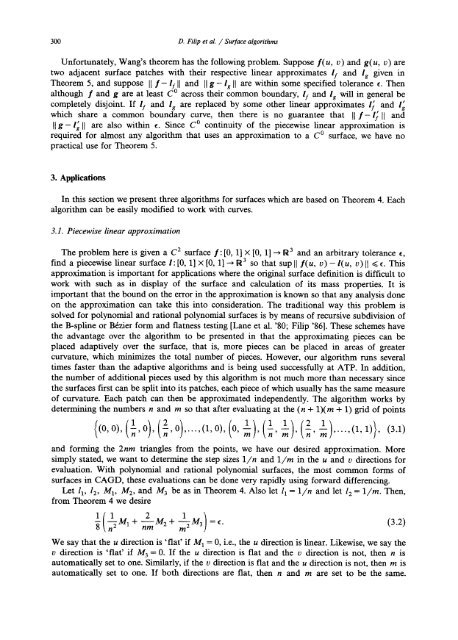
Unfortunately, Wang's theorem has the following problem. Suppose f(u, v) and g(u, v) are
two adjacent surface patches with their respective linear approximates ly and Ig given in
Theorem 5, and suppose [1 f- If I[ and [[ g - i s [I are within some specified tolerance c. Then
although f and g are at least C o across their common boundary, l! and lg will in general be
completely disjoint. If ! I and I s are replaced by some other linear approximates ! S and l~
which share a common boundary curve, then there is no guarantee that I[ f-IS [[ and
I[ g- ! s [[ are also within e. Since C O continuity of the piecewise linear approximation is
required for almost any algorithm that uses an approximation to a C O surface, we have no
practical use for Theorem 5.
3. Applications
In this section we present three <strong>algorithms</strong> for surfaces which are based on Theorem 4. Each
algorithm can be easily modified to work with curves.
3.1. Piecewise linear approximation
The problem here is given a C 2 surface f: [0, 1] × [0, 1] ~ R 3 and an arbitrary tolerance c,
find a piecewise linear surface l: [0, 1] × [0, 1] ~ R 3 so that sup II l(u, v) - l(u, v)II < c. This
approximation is important for applications where the original surface definition is difficult to
work with such as in display of the surface and calculation of its mass properties. It is
important that the bound on the error in the approximation is known so that any analysis done
on the approximation can take this into consideration. The traditional way this problem is
solved for polynomial and rational polynomial surfaces is by means of recursive subdivision of
the B-spline or B6zier form and flatness testing [Lane et al. '80; Filip '86]. These schemes have
the advantage over the algorithm to be presented in that the approximating pieces can be
placed adaptively over the surface, that is, more pieces can be placed in areas of greater
curvature, which minimizes the total number of pieces. However, our algorithm runs several
times faster than the adaptive <strong>algorithms</strong> and is being used successfully at ATP. In addition,
the number of additional pieces used by this algorithm is not much more than necessary since
the surfaces first can be split into its patches, each piece of which usually has the same measure
of curvature. Each patch can then be approximated independently. The algorithm works by
determining the numbers n and m so that after evaluating at the (n + 1)(m + 1) grid of points
{( ) (1)(2 O) ( ) (__1) (1 1)(2 __1) ..,(1,1)}, (3.1)
0,0, ,0 , , ,..., 1,0, 0, m . . . . m '"
and forming the 2nm triangles from the points, we have our desired approximation. More
simply stated, we want to determine the step sizes 1/n and 1/m in the u and v directions for
evaluation. With polynomial and rational polynomial surfaces, the most common forms of
surfaces in CAGD, these evaluations can be done very rapidly <strong>using</strong> forward differencing.
Let l 1, l 2, M 1, M 2, and M 3 be as in Theorem 4. Also let l I = 1/n and let l 2 = 1/m. Then,
from Theorem 4 we desire
-8 MI+ nm 2+ M 3 =c. (3.2)
We say that the u direction is 'flat' if M 1 = O, i.e., the u direction is linear. Likewise, we say the
v direction is 'fiat' if M 3 = O. If the u direction is flat and the v direction is not, then n is
automatically set to one. Similarly, if the v direction is flat and the u direction is not, then m is
automatically set to one. If both directions are flat, then n and m are set to be the same.