Popinet S., Free computational fluid dynamics.pdf
Popinet S., Free computational fluid dynamics.pdf
Popinet S., Free computational fluid dynamics.pdf

Create successful ePaper yourself
Turn your PDF publications into a flip-book with our unique Google optimized e-Paper software.
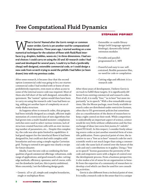
<strong>Free</strong> Computational Fluid Dynamics<br />
What is Gerris? Named after the Gerris remigis or common<br />
water strider, Gerris is yet another tool for <strong>computational</strong><br />
<strong>fluid</strong> <strong>dynamics</strong>. Three years ago, I started working on a new<br />
numerical technique for the solution of flows with <strong>fluid</strong>/<strong>fluid</strong> interfaces<br />
(e.g. droplets, bubbles, waves etc.) in three dimensions. I had several<br />
choices: I could carry on using the 2D and 3D research codes I had<br />
used and developed for several years, I could try to find a (preferably<br />
cheap) well-designed, extensible commercial code, or I could design a<br />
new code from scratch trying to avoid the pitfalls I had fallen (or been<br />
drawn) into with my previous codes.<br />
After some research, it became clear that the second<br />
option (commercial code) was going to be a no-starter:<br />
commercial codes I had worked with or knew of were<br />
prohibitively expensive, even more so when access to<br />
some of the internal source code was required. Most of<br />
them also fell short of the well-designed, extensible requirement.<br />
�e “easiest” option would then have been<br />
to carry on using the research code I was had been using,<br />
adding yet another layer of complexity on an already<br />
shaky structure.<br />
As happens often to research codes, this program<br />
had been initially designed as a simple, efficient implementation<br />
of a restricted class of new algorithms but<br />
had grown into a multi-headed monster: compilation<br />
switches were used to select various versions, lack of<br />
structure created function calls with an ever-increasing<br />
number of parameters, etc... Despite this complexity,<br />
the code was also quite limited in capabilities: it<br />
had good support for the interfacial flows it had been<br />
designed for, but could not deal with complex solid<br />
boundaries and was using a simple regular Cartesian<br />
grid. Trying to extend it yet again was clearly a recipe<br />
for future disaster.<br />
Ideally, I saw the new code as combining the best<br />
qualities of good commercial offerings: robustness, wide<br />
range of applications; and good research codes: cuttingedge<br />
methods, efficiency, openness; and of course, without<br />
the drawbacks (and yes, this is pretty ambitious).<br />
More concretely, I set the following design goals:<br />
• Generic: 2D or 3D, simple and complex boundaries,<br />
single or multiphase flows<br />
2 CLUSTERWORLD volume 2 no 6<br />
STÈPHANE POPINET<br />
• Extensible: re-usable library<br />
design (with language-agnostic<br />
bindings), dynamically-linked<br />
extension modules<br />
• Portable and parallel:<br />
programmed in C, MPI<br />
• Powerful and easy to use: self-<br />
contained, flexible parameter files,<br />
no-need for code re-compilation<br />
• Cutting-edge and efficient: it is a<br />
research code<br />
After three years of development, I believe Gerris is<br />
on track to fulfill these targets. It is significantly different<br />
from existing commercial and research codes.<br />
First of all, it is really “free,” “as in beer” but more importantly<br />
“as in speech.” With a few remarkable exceptions,<br />
like the Mouse package, most freely available research<br />
codes are distributed under restrictive licenses,<br />
often due to US-government policies but sometimes<br />
also as a manifestation of the desire of researchers to<br />
keep a tight control on their work. While competition<br />
is undoubtedly an important aspect of science, science<br />
would do very little without collaboration and the free<br />
exchange of ideas (see www.lmm.jussieu.fr/~zaleski/<br />
OpenCFD.html). In this respect, I consider freely releasing<br />
source codes as just another essential form of scientific<br />
publication. From a practical point of view, the incentive<br />
to use a “free as in beer” research code for one’s<br />
scientific work is not much larger than using a commercial<br />
code: the same lack of control over the future of the<br />
code and one’s contributions to it applies. Using a “free<br />
as in speech” license guarantees the perennity of the<br />
code and empowers users with a degree of control over<br />
the development process. From a business perspective,<br />
it also makes a lot of sense for an organization to benefit<br />
from the expertise of a community of researchers to<br />
develop a tool which can then be used for core consulting<br />
activities.<br />
Gerris is also different from a technical point of view.<br />
It is really a research code in the sense that it is a unique
combination of recent new approaches in CFD. While<br />
most modern solvers are based on fully-unstructured<br />
meshes, Gerris uses semi-structured quadtree/octree<br />
meshes. �is type of discretization is a good compromise<br />
between the flexibility of unstructured meshes and the<br />
<strong>computational</strong> efficiency of structured meshes. �e main<br />
problem with this approach is that the discretized elements<br />
cannot generally be made to follow the boundaries<br />
of complex domains. To overcome this difficulty,<br />
Gerris uses an embedded solid boundary representation<br />
where cells cut by solid boundaries are treated differently<br />
in order to apply boundary conditions accurately. An<br />
important practical consequence of this approach is that<br />
the often difficult and time-consuming first step of domain<br />
meshing (for unstructured meshes) can be entirely<br />
automated. Better still, the quad/octree mesh creation<br />
process is efficient enough to be applicable at every time<br />
step with little penalty. �e solver can then adapt the<br />
mesh dynamically to the solution being computed. �is<br />
result can lead to huge improvements in computation<br />
time and/or solution quality.<br />
Current Capabilities<br />
Time-dependent incompressible flows are the primary<br />
focus. Figure One illustrates an example of 3D Euler<br />
incompressible turbulent air flow around the research<br />
vessel Tangaroa of NIWA. �e time-adaptive mesh of<br />
Figure Two is used to discretize the solution dynamically.<br />
We also validated the numerical results using insitu<br />
wind measurements. �e meshed CAD model of<br />
the vessel was imported directly into Gerris and used<br />
for automatic mesh generation. �e code can also solve<br />
variable-density flows, advection-diffusion equations<br />
(e.g. passive tracers). Two-phase flows can be treated<br />
using a Volume Of Fluid (VOF) advection scheme in 2D<br />
and 3D. Stokes and Navier-Stokes flows are for the moment<br />
restricted to 2D.<br />
An Example<br />
After this general overview, let’s look at how Gerris<br />
works in practice.<br />
I will first assume that you have installed all the required<br />
components (see the Sidebar).<br />
As a first example we will setup a Navier-Stokes simulation<br />
of a 2D flow around a circular cylinder. �e flow will<br />
be from left to right, with the cylinder placed in a straight<br />
channel eight times longer than it is wide. A passive tracer<br />
will be injected at the inlet to visualize the flow. We will<br />
also use dynamic adaptive mesh refinement.<br />
Gerris is a command line-oriented program. �e code<br />
is controlled through a parameter file. One of the design<br />
goals was that every aspect of the simulation should be<br />
COMPUTATIONAL FLUID DYNAMICS<br />
FIGURE ONE Snapshot of the simulation of a 3D air flow around a<br />
CAD model of the research vessel Tangaroa. �e colors represent<br />
the local amplitude of the wind speed.<br />
FIGURE TWO Vertical and horizontal cross sections showing the<br />
adaptive mesh used to resolve the flow<br />
controllable through the parameter file without any need<br />
for recompilation or tinkering within the code.<br />
Let’s first define the simulation domain. Fire up<br />
your favorite text editor and copy the following:<br />
8 7 GfsSimulation GfsBox GfsGEdge {} {<br />
}<br />
GfsBox {}<br />
GfsBox {}<br />
GfsBox {}<br />
GfsBox {}<br />
GfsBox {}<br />
GfsBox {}<br />
GfsBox {}<br />
GfsBox {}<br />
1 2 right<br />
2 3 right<br />
3 4 right<br />
4 5 right<br />
5 6 right<br />
6 7 right<br />
7 8 right<br />
volume 2 no 6 CLUSTERWORLD 3
COMPUTATIONAL FLUID DYNAMICS<br />
�is defines the computation domain as a graph (of<br />
type GfsSimulation) of eight nodes (of type Gfs-<br />
Box) linked by seven edges (of type GfsGEdge ). Each<br />
of the nodes is then defined (the eight lines starting<br />
with GfsBox) and each of the edges (the seven lines<br />
ending with right). �e edges are simply defined by<br />
the indexes of the nodes they are connecting together<br />
with the direction in which the connection is done<br />
(right, left, top, bottom). All the blocks delimited by<br />
braces are placeholders for optional parameters. A<br />
GfsBox is simply a square domain (cube in 3D) of size<br />
unity. �is parameter file thus defines a rectangular domain<br />
of size 8x1.<br />
What about boundary conditions? If left unspecified,<br />
the default is a “mirror” or symmetry condition for<br />
all fields. �at will do fine for the sides of the channel<br />
(a friction-free solid wall) but we want to impose a constant<br />
inflow velocity on the left-side of the channel and<br />
an outflow condition on the right side. We can do that<br />
easily by adding the following arguments to the first<br />
and last nodes:<br />
8 7 GfsSimulation GfsBox GfsGEdge {} {<br />
}<br />
GfsBox {<br />
left = GfsBoundary {<br />
GfsBcDirichlet U 1<br />
}<br />
}<br />
...<br />
GfsBox { right = GfsBoundaryOutflow }<br />
�is defines the right side of the last node as a Gfs-<br />
BoundaryOutflow and the left side of the first node<br />
as a generic GfsBoundary. A GfsBoundary takes extra<br />
optional arguments defining the boundary conditions<br />
variable by variable. �e GfsBcDirichlet U 1<br />
line sets this left-side boundary as a Dirichlet (fixed<br />
value) boundary condition of 1 for the U variable (the<br />
horizontal component of the velocity). We also want to<br />
inject some tracer at the inlet. �is can be done by adding<br />
a boundary condition for a C variable, like this:<br />
...<br />
left = GfsBoundary {<br />
GfsBcDirichlet U 1<br />
GfsBcDirichlet C { return y < 0. ? 1. : 0.; }<br />
}<br />
...<br />
�is is similar to the boundary condition for U but here<br />
we have used a powerful feature of the parameter file<br />
4 CLUSTERWORLD volume 2 no 6<br />
system: the possibility to specify most numeric arguments<br />
as functions of space (x,y,z) and time t. �e functions<br />
are written as C functions (you will thus need<br />
some basic notion of the C language to use them). By<br />
convention the first GfsBox of the graph is centered on<br />
the origin (x = y = 0). �e boundary condition we wrote<br />
just sets C to 1 in the lower half of the boundary (y < 0.)<br />
and to zero otherwise.<br />
For the moment we have not told the code how to discretize<br />
our domain (how many grid points we want and so<br />
on), for how long the simulation should run and what the<br />
initial conditions are. �is can be done by adding:<br />
8 7 GfsSimulation GfsBox GfsGEdge {} {<br />
GfsTime { end = 15 }<br />
GfsRefine 6<br />
GfsInit {} { U = 1 }<br />
}<br />
...<br />
�e argument to GfsRefine is the number of quadtree<br />
levels the code should use to discretize each GfsBox.<br />
In our case 6, which will give 2^6=64 grid points in the<br />
width of the channel. �is argument could also be a function<br />
of space if we wanted a non-uniform mesh. �e line<br />
starting with GfsInit specifies the boundary conditions<br />
for each variable. In our case we just set U to 1 everywhere<br />
in the domain, all the other variables are zero by default.<br />
�is file is enough to run a (pretty boring) simulation:<br />
uniform flow in a channel and more problematically no<br />
outputs! Outputs are controlled by a number of objects all<br />
derived from a GfsOutput parent class. Several objects<br />
are provided with Gerris to output various things one may<br />
be interested in. For advanced users, it is also easy (with<br />
some knowledge of C programming) to define one’s custom<br />
new output object with very few limitations on what<br />
can be done. Let’s add a few to our parameter file:<br />
8 7 GfsSimulation GfsBox GfsGEdge {} {<br />
GfsTime { end = 15 }<br />
GfsRefine 6<br />
GfsInit {} { U = 1 }<br />
GfsOutputTime { istep = 10 } stdout<br />
GfsOutputBalance { istep = 10 } stdout<br />
GfsOutputProjectionStats { istep = 10 }<br />
stdout<br />
GfsOutputPPM { istep = 2 } vort.ppm {<br />
min = -10 max = 10 v = Vorticity<br />
}<br />
GfsOutputPPM { istep = 2 } c.ppm {<br />
min = 0 max = 1 v = C<br />
}
GfsOutputTiming { start = end } stdout<br />
}<br />
...<br />
All output objects share a similar structure. �e first<br />
optional argument defines the time window and recurrence<br />
of the output “event”. Units are either physical<br />
time or number of time steps taken. For example<br />
istep = 2 means “output every second time step”<br />
while step = 2 would mean “output every two physical<br />
time units.” Similarly start = end means “execute<br />
this only once at the end of the simulation.” �e<br />
second argument tells the code where to write the resulting<br />
output, it can be a file name or a pipe (more on<br />
this later). �e file names stdout and stderr have<br />
special meaning as the standard output and standard<br />
error respectively. GfsOutputTime writes the current<br />
iteration and physical time, GfsOutputBalance gives<br />
statistics on the number of grid points, GfsOutput-<br />
ProjectionStats statistics on the convergence rate<br />
of the solver. GfsOutputPPM is more interesting. It<br />
produces a PPM (Portable PixMap) bitmap image of the<br />
field given by the v = parameter.<br />
�ere are still three things missing from our parameter<br />
file: the cylinder, adaptive mesh refinement<br />
and <strong>fluid</strong> viscosity. To define solid boundaries, Gerris<br />
needs a “triangulated surface” as input: that is, a surface<br />
mesh composed of triangular elements. �is mesh<br />
needs to be a “proper” surface: i.e. it must be closed (no<br />
gaps, however small), it must not be folded on itself,<br />
etc... �is is very much the same type of requirement as<br />
for most unstructured mesh generators. Unfortunately,<br />
many Computer Aided Design (CAD) packages do not<br />
always produce well-behaved surfaces (they may look<br />
good on screen but are full of tiny cracks and folds).<br />
�ere consequently is a whole industry of software<br />
dealing purely with “mesh repair”. For our example, I<br />
will just provide you with a proper triangulated mesh<br />
of a cylinder (see Resources). Gerris expects files to be<br />
in the GTS (GNU Triangulated Surface) format, a simple<br />
text format. �e distribution also comes with a few<br />
conversion utilities (such as dxf2gts which converts<br />
AutoCad triangulated surfaces to the GTS format). To<br />
add this solid boundary to the simulation just copy the<br />
GTS file to the working directory and add the following<br />
to the parameter file:<br />
...<br />
GtsSurfaceFile cylinder.gts<br />
...<br />
Adaptive refinement and viscosity are controlled by<br />
adding<br />
...<br />
GfsAdaptVorticity { istep = 1 } {<br />
maxlevel = 6 cmax = 1e-2 }<br />
GfsAdaptGradient { istep = 1 } {<br />
maxlevel = 6 cmax = 1e-2 } C<br />
GfsSourceViscosity {} U 0.00078125<br />
...<br />
We use two criteria to control mesh adaptation: the<br />
vorticity (i.e. “rate of rotation”) of the flow field and the<br />
gradient of the passive tracer C. In both cases adaptation<br />
is performed at every timestep { istep = 1 },<br />
the maximum number of refinement levels allowed is<br />
6 (if unspecified the minimum level is 1). �e refinement<br />
stops whenever the criterion becomes smaller<br />
than cmax.<br />
�e viscosity nu we set corresponds to a Reynolds<br />
number Re=UD/nu of 160. Where U is the inflow velocity<br />
(1 in our case), D is the diameter of the cylinder (1/8<br />
of the channel width).<br />
Everything is now ready, just save the file as<br />
cylinder.sim and on the command line type:<br />
$ gerris2D cylinder.sim<br />
If you have not made any typos, the code should run,<br />
writing information on the screen every ten time steps.<br />
If in another terminal you now type<br />
$ animate vort.ppm<br />
or<br />
$ animate c.ppm<br />
COMPUTATIONAL FLUID DYNAMICS<br />
you will be able to follow graphically the progress of<br />
the simulation (note that animate does not automatically<br />
re-read the PPM file as the simulation progresses,<br />
you need to restart it).<br />
What you will find is that the PPM files grow quite<br />
quickly. �e PPM file format is portable and very simple<br />
but no compression at all is used which makes it<br />
quite inefficient as a storage format (even more so for<br />
movies). Generating an MPEG movie would be nice.<br />
One solution would be to wait for the end of the simulation<br />
and then convert the PPM files to MPEG files<br />
using some conversion tool. A better solution (which<br />
will not generate large temporary files) is to do the<br />
conversion “on the fly.” Using the powerful “pipe” feature<br />
of the parameter file and the right conversion tool<br />
(MJPEG Tools) it is very easy to do. Just change the relevant<br />
lines in the parameter file to:<br />
volume 2 no 6 CLUSTERWORLD 5
COMPUTATIONAL FLUID DYNAMICS<br />
...<br />
GfsOutputPPM { istep = 2 } { ppmtoy4m -F<br />
24:1 -v 0 | mpeg2enc -v 0 -o vort.mpg } {<br />
min = -10 max = 10 v = Vorticity<br />
}<br />
GfsOutputPPM { istep = 2 } { ppmtoy4m -F<br />
24:1 -v 0 | mpeg2enc -v 0 -o c.mpg } {<br />
min = 0 max = 1 v = C<br />
}<br />
...<br />
GfsOutputPPM will do the same thing as before but instead<br />
of directly writing the result to a file, it will pipe<br />
the PPM image into the ppmtoy4m and mpeg2enc commands<br />
(themselves connected by a pipe) and directly<br />
generate a MPEG file. �is is just an example of how a<br />
running Gerris simulation can be connected to various<br />
post-processing tools, visualization etc. ...<br />
With this improvement done, you probably want to<br />
stop the running simulation (Ctrl-c will do) and rerun<br />
it with the improved parameter file. �e MPEG files generated<br />
can then be visualized using your favorite player.<br />
If you are patient (15 to 30 minutes waiting time)<br />
you will get to the stage of the fully developed Von Karman<br />
vortex street pictured in Figure �ree.<br />
More on post-processing<br />
For the moment we have only used very simple builtin<br />
“post”-processing of the simulation results. �ere<br />
are several other post-processing options built into the<br />
Gerris code base but for more sophisticated visualizations<br />
(particularly in 3D), it is better to use other packages<br />
dedicated to visualization. Unfortunately, all the<br />
packages I have tested are systematically geared toward<br />
either structured (Cartesian-like) or fully-unstructured<br />
meshes (triangular or quadrilateral elements in 2D,<br />
tetrahedra in 3D) and thus do not take full advantage<br />
of the multiscale representation automatically given by<br />
the semi-structured approach used by Gerris (see sidebar<br />
for details).<br />
To use an external visualization tool, the first step<br />
is to save the results of the simulation for the time<br />
steps we are interested in. �is can be done by adding:<br />
FIGURE THREE Von Karman vortex street behind a cylinder. Vor-<br />
ticity field (top) and passive tracer (bottom).<br />
6 CLUSTERWORLD volume 2 no 6<br />
...<br />
GfsOutputSimulation { start = 1 step = 1<br />
} cylinder-%02.0f.sim {}<br />
...<br />
If you then restart the simulation, it will now save files<br />
called cylinder-01.sim , cylinder-02.sim , ...,<br />
cylinder-15.sim . �ese files contain all that is necessary<br />
to restart the simulation. If you open one in your<br />
text editor you will see that it is very similar to your<br />
cylinder.sim parameter file apart from a large section<br />
containing the detail of the discretization and values of<br />
the variables. You can of course change some of the parameters,<br />
add outputs etc... and restart the simulation<br />
from where it stopped with the updated file.<br />
Gerris comes with several filters that can convert<br />
simulation files to formats readable by external visualization<br />
programs. For development I mostly use a<br />
slightly crufty filter called gfs2oogl in combination<br />
with Geomview. Geomview is a nice generic 3D object<br />
viewer with a number of interesting features but is not<br />
geared specifically toward scientific visualization. Most<br />
of the work is thus done by the filter itself. As an example<br />
just try the following:<br />
$ gfs2oogl2D < cylinder-15.sim ><br />
cylinder-15.oogl<br />
$ geomview cylinder-15.oogl<br />
With some panning and zooming you should get an reasonable<br />
image. Gfs2oogl can do much more than this<br />
but is not very user-friendly: try $ gfs2oogl2D -h for<br />
a brief overview of the various options.<br />
For a more graphical experience, you can try the excellent<br />
MayaVi, which is geared specially toward flow<br />
visualization. It can do classical things like cross-sections,<br />
isosurfaces, vector plots etc... �e gfs2vtk filter<br />
can be used to generate VTK (Visualization Tool Kit)<br />
files readable by MayaVi. Try the following:<br />
$ gfs2vtk2D cylinder-15 < cylinder-15.sim<br />
$ mayavi -d cylinder-15_field.vtk<br />
Click on the “Configure Data” button, select scalar “C”<br />
on the pop-up window, click on the “Visualize -> Modules<br />
-> SurfaceMap” menu entry and you should get<br />
your first Mayavi visualization.<br />
For a very powerful but relatively heavy graphical<br />
visualization tool, you can try IBM’s open-source<br />
OpenDX. �is is more a graphical programming environment<br />
(modules linked graphically by pipes) than a
stand-alone visualization tool. It is also very powerful.<br />
Gerris comes with a special OpenDX module that<br />
can be used to import simulation files directly into<br />
OpenDX. To use it, start OpenDX like this:<br />
$ dx -mdf /usr/local/lib/gerris/dx2D.mdf<br />
If you are not familiar with OpenDX you should then<br />
read the extensive documentation.<br />
Parallel Computation<br />
Gerris was designed from scratch with parallel computation<br />
in mind. I chose a simple domain decomposition<br />
approach, which is one of the main reason of the<br />
slightly weird graph structure of the domain definition<br />
in parameter files.<br />
Let’s come back to our 2D example. Suppose you<br />
want to use 8 processors of your parallel machine. For<br />
the domain we have, a fairly obvious decomposition<br />
strategy is just to assign each of the eight GfsBox to<br />
each processor. �is can be done easily by modifying<br />
the parameter file like this:<br />
...<br />
GfsBox { pid = 0 }<br />
GfsBox { pid = 1 }<br />
GfsBox { pid = 2 }<br />
GfsBox { pid = 3 }<br />
GfsBox { pid = 4 }<br />
GfsBox { pid = 5 }<br />
GfsBox { pid = 6 }<br />
GfsBox { pid = 7 }<br />
...<br />
�e simulation can then be ran on eight processors like<br />
this:<br />
$ mpirun -np 8 gerris2D cylinder.sim<br />
�e simulation file can still be run on a single processor<br />
as usual (the pid info is just ignored).<br />
What is currently lacking is a parallel output capability.<br />
�e files written by each processor are entirely<br />
independent (i.e. they represent only the part of the<br />
domain simulated by this processor). It is then up to<br />
you to put the puzzle back together.<br />
What we did is an example of manually partitioning<br />
the domain. In more complex cases, Gerris can also<br />
automatically partition the domain for a given number<br />
of processors, variable resolution, complex boundaries<br />
etc. It does this using sophisticated I<br />
algorithms which aim to minimize the cost of<br />
Resources<br />
COMPUTATIONAL FLUID DYNAMICS<br />
Gerris: gfs.sf.net<br />
GTS: gts.sf.net<br />
Glib: www.gtk.org<br />
Mouse: www.vug.uni-duisburg.de/MOUSE<br />
Triangulated mesh of a cylinder:<br />
gfs.sourceforge.net/clusterworld<br />
OpenDX: www.opendx.org<br />
Mayavi: mayavi.sf.net<br />
Geomview: www.geomview.org<br />
ImageMagick: www.imagemagick.org<br />
MJPEG Tools: mjpeg.sf.net<br />
communications between sub-domains. �is is done in<br />
two steps. Let’s say we want to now run our simulation<br />
on 32 processors. Just type:<br />
$ gerris2D -p 5 cylinder.sim > cylinder-32.sim<br />
�is will create a new simulation file which can the be<br />
run on 32 processors. �e -p option is the power of two<br />
processors, in this case two to the fifth power.<br />
Apart from parallel outputs, the main issue which<br />
is not currently addressed by Gerris is dynamic loadbalancing<br />
which is necessary to keep good parallel efficiency<br />
when adaptive mesh refinement is used.<br />
The Future of Gerris<br />
As you have probably found out by now, while Gerris<br />
seems to be on the right track there is still a lot to be<br />
done to take full advantage of its flexibility. Together<br />
with collaborators at NIWA and elsewhere, I am currently<br />
working on several aspects of the code. �e first shortterm<br />
goal is to extend the Navier-Stokes and diffusion<br />
equations solution to three dimensions. �is is made<br />
slightly more difficult by the treatment of embedded<br />
Dirichlet boundary conditions in three-dimensions.<br />
Another active area is the development of non-newtonian<br />
viscous stresses (i.e. <strong>fluid</strong>s for which the stress/<br />
strain relationship is not linear): applications include<br />
the numerical simulation of visco-plastic <strong>fluid</strong>s (e.g.<br />
snow and mud avalanches, granular materials, plastics)<br />
and Large-Eddy-Simulations (LES) turbulence modeling.<br />
A very recent endeavor has been the extension of<br />
Gerris to geophysical <strong>fluid</strong> <strong>dynamics</strong> i.e. oceanic and<br />
atmospheric flows, where the adaptive mesh approach<br />
has proved extremely useful.<br />
Potential extensions which would make full use<br />
of the existing framework are numerous. Just a few<br />
ideas including; steady-state flow solvers, compressible<br />
volume 2 no 6 CLUSTERWORLD 7
COMPUTATIONAL FLUID DYNAMICS<br />
flows, and Python bindings.<br />
In addition, the hierarchical quadtree/octree meshes<br />
used by Gerris allows for a true multi-scale representation<br />
of the solution. Visualization would greatly<br />
benefit from this, particularly for large 3D simulations.<br />
Unfortunately, I am not aware of any existing visualization<br />
tool designed to take advantage of this. If you<br />
like writing visualization programs and want to contribute<br />
a cutting-edge visualization tool, you will gain<br />
the eternal gratitude of Gerris users!<br />
Whether all or none of these extensions happen depends<br />
on the community of Gerris users. I hope that<br />
you have found Gerris appealing and that you will con-<br />
Installing Gerris<br />
Gerris is written in C and uses two other C libraries<br />
which you need to install on your system first; the<br />
Glib library and the GTS library. If you want to run the<br />
parallel version of Gerris, you will also need some implementation<br />
of the MPI (Message Passing Interface) library.<br />
Gerris is quite portable and has been tested on Linux<br />
clusters, CRAY T3E parallel computer, HP and Silicon<br />
Graphics workstations. If you are using a Linux system the<br />
Glib library is most probably already installed on your system.<br />
To be sure try this:<br />
$ glib-config --version<br />
If you get a result, you have the Glib library on your system,<br />
otherwise you will need to install it following the instructions<br />
on the Glib web site.<br />
You now need to install the GNU Triangulated Surface<br />
Library (GTS). To do that, go on the GTS web site<br />
and download a recent source file package. Move it to<br />
your preferred location for unpacking source files and<br />
type:<br />
$ gunzip gts.tar.gz<br />
$ tar xvf gts.tar<br />
$ cd gts<br />
You now need to decide where you want to install the library,<br />
if you have access to the root account, you can simply<br />
type:<br />
$ ./configure<br />
$ make<br />
$ su<br />
$ make install<br />
$ exit<br />
8 CLUSTERWORLD volume 2 no 6<br />
sider contributing the missing features you wish it had.<br />
And remember, the beauty of (really) free software is<br />
that whatever happens, your contribution will always<br />
be there for you (and others) to share.<br />
Acknowledgments<br />
Gerris was made possible by the support of the National<br />
Institute of Water and Atmospheric research (NIWA) and<br />
the Marsden Fund of the Royal Society of New Zealand.<br />
StÈphane <strong>Popinet</strong> is a research scientist at the National Institute<br />
of Water and Atmospheric research, Wellington, New Zealand.<br />
He can be reached at s.popinet@niwa.cri.nz.<br />
which will install everything in /usr/local by default. If<br />
you don’t have access to the root password or want to install<br />
the library somewhere else like /home/joe/local for example,<br />
you can type instead:<br />
$ ./configure --prefix=/home/joe/<br />
local<br />
$ make<br />
$ make install<br />
You probably want to add /home/joe/local/bin to<br />
your PATH and /home/joe/local/lib to your LD_<br />
LIBRARY_PATH . The next step is installing Gerris itself,<br />
do the same, go to the Gerris web site download a recent<br />
source file package and type:<br />
$ gunzip gerris.tar.gz<br />
$ tar xvf gerris.tar<br />
$ cd gerris<br />
$ ./configure --prefix=/home/joe/local<br />
$ make<br />
$ make install<br />
Both the 2D and 3D versions of the code are built. We are<br />
now ready to start. Just to check that everything is working<br />
try:<br />
$ gerris2D -V<br />
For visualization you probably also want to use the ImageMagick<br />
tools (which are installed by default on most<br />
Linux distributions) as well as Geomview, Mayavi or<br />
OpenDX. We will also make use of the MJPEG Tools for<br />
the generation of MPEG movies.<br />
Note that Gerris will compile and install the OpenDX<br />
modules only if OpenDX was installed on your system before<br />
compiling Gerris.