Surface algorithms using bounds on derivatives

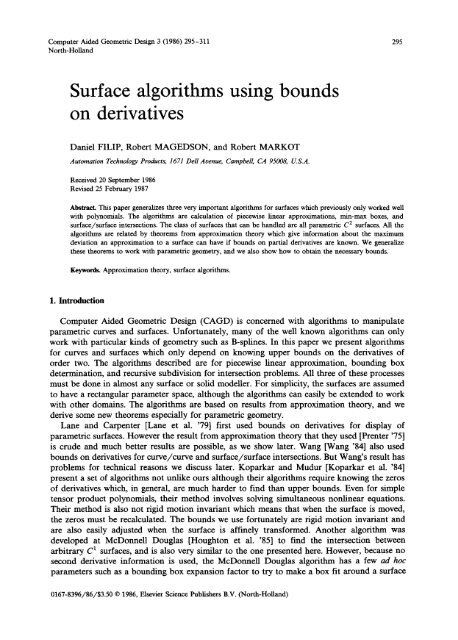
Computer Aided Geometric Design 3 (1986) 295-311 295 

North-Holland 

<strong>Surface</strong> <strong>algorithms</strong> <strong>using</strong> <strong>bounds</strong> 

on derivatives 

Daniel FILIP, Robert MAGEDSON, and Robert MARKOT 

Automation Technology Products, 1671 Dell Aoenue, Campbell, CA 95008, U.S.A. 

Received 20 September 1986 

Revised 25 February 1987 

Abstract. This paper generalizes three very important <strong>algorithms</strong> for surfaces which previously only worked well 

with polynomials. The <strong>algorithms</strong> are calculation of piecewise linear approximations, min-max boxes, and 

surface/surface intersections. The class of surfaces that can be handled are all parametric C 2 surfaces. All the 

<strong>algorithms</strong> are related by theorems from approximation theory which give information about the maximum 

deviation an approximation to a surface can have if <strong>bounds</strong> on partial derivatives are known. We generalize 

these theorems to work with parametric geometry, and we also show how to obtain the necessary <strong>bounds</strong>. 

Keywords. Approximation theory, surface <strong>algorithms</strong>. 

1. Introduction 

Computer Aided Geometric Design (CAGD) is concerned with <strong>algorithms</strong> to manipulate 

parametric curves and surfaces. Unfortunately, many of the well known <strong>algorithms</strong> can only 

work with particular kinds of geometry such as B-splines. In this paper we present <strong>algorithms</strong> 

for curves and surfaces which only depend on knowing upper <strong>bounds</strong> on the derivatives of 

order two. The <strong>algorithms</strong> described are for piecewise linear approximation, bounding box 

determination, and recursive subdivision for intersection problems. All three of these processes 

must be done in almost any surface or solid modeller. For simplicity, the surfaces are assumed 

to have a rectangular parameter space, although the <strong>algorithms</strong> can easily be extended to work 

with other domains. The <strong>algorithms</strong> are based on results from approximation theory, and we 

derive some new theorems especially for parametric geometry. 

Lane and Carpenter [Lane et al. '79] first used <strong>bounds</strong> on derivatives for display of 

parametric surfaces. However the result from approximation theory that they used [Prenter '75] 

is crude and much better results are possible, as we show later. Wang [Wang '84] also used 

<strong>bounds</strong> on derivatives for curve/curve and surface/surface intersections. But Wang's result has 

problems for technical reasons we discuss later. Koparkar and Mudur [Koparkar et al. '84] 

present a set of <strong>algorithms</strong> not unlike ours although their <strong>algorithms</strong> require knowing the zeros 

of derivatives which, in general, are much harder to find than upper <strong>bounds</strong>. Even for simple 

tensor product polynomials, their method involves solving simultaneous nonlinear equations. 

Their method is also not rigid motion invariant which means that when the surface is moved, 

the zeros must be recalculated. The <strong>bounds</strong> we use fortunately are rigid motion invariant and 

are also easily adjusted when the surface is affinely transformed. Another algorithm was 

developed at McDonnell Douglas [Houghton et al. '85] to find the intersection between 

arbitrary C 1 surfaces, and is also very similar to the one presented here. However, because no 

second derivative information is used, the McDonnell Douglas algorithm has a few ad hoc 

parameters such as a bounding box expansion factor to try to make a box fit around a surface 

0167-8396/86/$3.50 © 1986, Elsevier Science Publishers B.V. (North-Holland)

296 D. Filip et aL / <strong>Surface</strong> <strong>algorithms</strong> 

and a surface normal ratio factor to try to determine surface flatness. The theory in this paper 

describes how to determine these factors very precisely. 

In Section 2 we develop the general theory needed, in Section 3, we give applications of the 

general theory, and in Section 4 we show how to compute the upper <strong>bounds</strong> needed for the 

<strong>algorithms</strong>. Section 5 derives another theorem to improve the <strong>algorithms</strong> in certain cases. 

2. General theory 

In this section we present some new and old approximation theoretic results for curves and 

surfaces. 

2.1. Approximating curves 

Wang used the following result for linearly approximating curves, which is proved in [de 

Boor '78, p. 39]: 

Theorem 1. Let f:[a, b]~ R be any C 2 function and let l(x) 

l(a) =f(a) and l(b)=f(b). Then 

sup If(x)-l(x)l

Which implies 

D. Filip et al. / <strong>Surface</strong> <strong>algorithms</strong> 297 

lie(to) 112~ < lie(to)II IlftS(a-x)l'(x) dxll, 

and since I[ e(to)II > 0 (if not we're done): 

lie(t0) [I ~ [[ft~( a- x).f'(x) dxl[ 

~

a

298 D. Filip et aL / <strong>Surface</strong> <strong>algorithms</strong> 

(a) 

B 

R 2 

A C A ~11 

Fig. 1. (a) The four regions of parameter triangle T used in the proof of Theorem 4, and (b) the region R 1 enlarged. 

where 

= 0 2i( u, o)l 

M1 (u,v)ETSUp an 2 ] , 

sup I°V(u'°), 

(u,o)~T OUOO 

343= sup 

L 

O2f(u' v). I 

(u,v)~T 0V2 l" 

Proof. Let e(u, v)=f(u, v)-l(u, v) and s(u, v)=e(u, v).e(u, v). Since T is compact, 

s(u, v) attains its maximum at some point P0 ~ T. If P0 lies on the boundary, then we can just 

apply Theorem 2 (taking special care if P0 is on the hypotenuse of T). So suppose P0 is in the 

interior of T. Then (3s/Ou)(po) = 0 = (3s/Ov)(po), which implies e(po) . (Oe/Ou)(Po) = 0 = 

e(po). (3e/Ov)(po). Also suppose Po ~ R1, as shown in Fig. 1, the other cases being proved 

similarly. Let v=A-Po and write v=(d cos 0, d sin 0) where d= IIA -P0 II and 0 is the 

angle between A C and v. The proof now follows similarly to that given for Theorem 2 by 

looking at the curve g(t) from Po to A on e(u, v). Let g(t) = e(Po + tv), so g(0) = e(Po) and 

g(1) = e(A). Writing g(t) in its Taylor series yields: 

which implies 

,(t) =,(0) + g'(0)t + 

g(a) = g(0) + g'(0) + 

and expanding out gives 

where 

e(A) = e(Po) + ( Oe(po) 

Ou 

1( 02! ( 

I = fo --'--~ Ou 

fotg"(f)(1 ~) d~, 

fo'g"(f)(1 f) d~, 

d cos 0 + )(Oe'P°-----------" d sin OI ~ + I 

0v / 

02I 

Po + ~v) d2 c°s20 + 2 3--~v (Po + t;v) d2 sin 0 cos 0 

+ Ov 202Izkpo + ~v)d 2 sin20)(1 -- ~) d~. 

Taking the dot product of the last expression with e(po), and noting the following equalities: 

e(Po) . (8e/au)(po) = 0 = e(Po) . (3e/3v)(po) and e( A) = 0, yields: 

O=e(Po) .e(po) + e(Po). I,

which implies 

II e(p0)II2< lie(p0)II II I II, 

and since II e(po)II > 0 (if not, we're done), we get 

II e(po) II < It 1 II 


(d 2 c0s2~ M l -4- 2d 2 sin 0 cos 8 M2 + d 2 sin28) I f01(1 - 4) d~] 

= ½(d 2 cos28 M 1 + 2d 2 sin 8 cos 8 ME + d 2 sin28). 

Now observing Fig. l(b), notice that d cos 8 < ½l 1 and d sin 8 ~< ½12. Therefore 

1 2 

II e(p0)II < ½(112M1 + 2~1112M2 + z12M3) 

= (l?M1 + 21112M2 + [] 

Barnhill and Gregory [BarnhiU et al. '72] proved a similar theorem for scalar-valued 

functions with more general norms. However, their proof is not easily extended to vector-val- 

ued functions because of its complexity. It is actually possible to extend Theorem 4 to more 

general norms, but we elected not to do so for simplicity and also because these norms are 

rarely used in CAGD. 

It is not difficult to adjust the <strong>bounds</strong> 3/1, M2, and M 3 when f is affinely transformed to a 

surface g, where 

In this case 

g(u, v) = Mf(u, v) + T. 

auaav ~v) < II auaav~V) I, 

~a+bg(u, 

a--.~-.-.a~vt " 

V) 

. = I[ M aa + bI ( u' 

MII aa+bf(u' 

where II M II is the norm of the matrix M and is equal to the largest eigenvalue of this 3 × 3 

matrix. If the affine transformation is a rigid body motion, then II M I1 equals one and so no 

change to the original <strong>bounds</strong> is needed. 

We now discuss one more theorem due to Wang [Wang '84] which is directly applied to 

rectangular surfaces, and does not require the patches to be split up into triangles. 

Theorem 5. Let R c R 2 be the rectangular region with vertices (A, B, C, D ) of the form 

B = A + (l 1, 0), C = A + (0, 12), and D = A + (11, 12). Let Jr: R ~ R 3 be any C 2 function, and 

let l(u, v) be the linearly parametrized quadrilateral with l(A)=I(A)- A, l(B)=Jr(B)+ zl, 

t(C) =Jr(C) +A, and l(D) =Jr(D) -A, where A = ¼(f(A) -Jr(B) -Jr(C) +Jr(D)). (lt is not 

hard to show that l(u, v) is planar.) Then 

where 

sup II Jr(u, v) -t(u, v)II < ---ff- V~ (l?M 1 + 2I, I:M~ + I~M3), 

(u,v)~R 

( a2x2 a2x3 t 

M 1=max 3u 2 , 3u 2 , ~ ], 

[I 02xl ], a2x2 

M2=max~la--~v [ I,[ a2x3 1 

OuOv 1' 

1 

M3=max av 2 , av 2 ' av 2 ]

300 D. Filip et al. / <strong>Surface</strong> <strong>algorithms</strong> 

Unfortunately, Wang's theorem has the following problem. Suppose f(u, v) and g(u, v) are 

two adjacent surface patches with their respective linear approximates ly and Ig given in 

Theorem 5, and suppose [1 f- If I[ and [[ g - i s [I are within some specified tolerance c. Then 

although f and g are at least C o across their common boundary, l! and lg will in general be 

completely disjoint. If ! I and I s are replaced by some other linear approximates ! S and l~ 

which share a common boundary curve, then there is no guarantee that I[ f-IS [[ and 

I[ g- ! s [[ are also within e. Since C O continuity of the piecewise linear approximation is 

required for almost any algorithm that uses an approximation to a C O surface, we have no 

practical use for Theorem 5. 

3. Applications 

In this section we present three <strong>algorithms</strong> for surfaces which are based on Theorem 4. Each 

algorithm can be easily modified to work with curves. 

3.1. Piecewise linear approximation 

The problem here is given a C 2 surface f: [0, 1] × [0, 1] ~ R 3 and an arbitrary tolerance c, 

find a piecewise linear surface l: [0, 1] × [0, 1] ~ R 3 so that sup II l(u, v) - l(u, v)II < c. This 

approximation is important for applications where the original surface definition is difficult to 

work with such as in display of the surface and calculation of its mass properties. It is 

important that the bound on the error in the approximation is known so that any analysis done 

on the approximation can take this into consideration. The traditional way this problem is 

solved for polynomial and rational polynomial surfaces is by means of recursive subdivision of 

the B-spline or B6zier form and flatness testing [Lane et al. '80; Filip '86]. These schemes have 

the advantage over the algorithm to be presented in that the approximating pieces can be 

placed adaptively over the surface, that is, more pieces can be placed in areas of greater 

curvature, which minimizes the total number of pieces. However, our algorithm runs several 

times faster than the adaptive <strong>algorithms</strong> and is being used successfully at ATP. In addition, 

the number of additional pieces used by this algorithm is not much more than necessary since 

the surfaces first can be split into its patches, each piece of which usually has the same measure 

of curvature. Each patch can then be approximated independently. The algorithm works by 

determining the numbers n and m so that after evaluating at the (n + 1)(m + 1) grid of points 

{( ) (1)(2 O) ( ) (__1) (1 1)(2 __1) ..,(1,1)}, (3.1) 

0,0, ,0 , , ,..., 1,0, 0, m . . . . m '" 

and forming the 2nm triangles from the points, we have our desired approximation. More 

simply stated, we want to determine the step sizes 1/n and 1/m in the u and v directions for 

evaluation. With polynomial and rational polynomial surfaces, the most common forms of 

surfaces in CAGD, these evaluations can be done very rapidly <strong>using</strong> forward differencing. 

Let l 1, l 2, M 1, M 2, and M 3 be as in Theorem 4. Also let l I = 1/n and let l 2 = 1/m. Then, 

from Theorem 4 we desire 

-8 MI+ nm 2+ M 3 =c. (3.2) 

We say that the u direction is 'flat' if M 1 = O, i.e., the u direction is linear. Likewise, we say the 

v direction is 'fiat' if M 3 = O. If the u direction is flat and the v direction is not, then n is 

automatically set to one. Similarly, if the v direction is flat and the u direction is not, then m is 

automatically set to one. If both directions are flat, then n and m are set to be the same.


Otherwise, the algorithm proportionally rolls in the mixed partial term M 2 into the number of 

steps in u and the number of steps in v based on the ratio M1/M 3. Thus we have four cases: 

Case 1: M 1 > 0 and M 3 > 0. Let k = 3/11/3/13, and set n/m = k, which means n = km. Then 

from equation (3.2) we have 

1 ( 1 M+ ~2 M + -l---2-M3/m] 

Solving for m we obtain 

Case 2: 

Solving for n we obtain 

Case 3: 

Case 4: 

km 2 2 

m = -~e ( M 1 + 2kM 2 + k2M3 ). 

.-~-(.. 

M 1 > 0 and M 3 = 0. Let m = 1. Then from equation (3.2) we have 

1 M 

M 1 = 0 and M 3 > 0. This is the same as Case 2 with the roles of n and m switched. 

M1 = 0 = M 3. This case is the same Case 1 with k = 1, i.e. 

n~--m= V/1 ~ ( M1+ 2 M2 + M3 ) 

Crack Prevention. Usually an object consists of many surfaces and if the object is continuous, 

then the piecewise linear approximation to the entire object is usually expected to be 

continuous. However, if the above algorithm is applied to two different adjacent surfaces 

independently, then cracks can appear between the linear approximations to adjacent surfaces 

[Filip '86]. This is caused by adjacent surfaces being subdivided to different depths. One simple 

way to eliminate this problem is to subdivide all the surfaces to the same depth as the patch 

that needs the most subdivision. The problem with this solution is that it will generate an 

unduly large number of approximating pieces if just one of the surfaces is highly curved. 

A much better solution to this problem is the following. First piecewise linearly approximate 

each boundary curve to the accuracy of c by applying the piecewise linear approximating 

scheme to the curve case. Then when evaluating the grid of points in set (3.1), if a point lies on 

the boundary of the surface, move it to the closest point on the approximation to the boundary. 

Since two adjacent surfaces share a common boundary curve, the approximation to that curve 

will be the same from both patches. So because boundary points are moved to that approxima- 

tion, no cracks will occur. One should notice that polygons from the approximation along the 

boundary may have more than three sides and may be non-planar (Fig. 2). These boundary 

polygons can easily be triangulated if required. It is very important to note, however, that the 

resulting approximation may not be within c in the neighborhood of the boundary curves. One 

way to get around this problem is to approximate the boundary curves and the surfaces to a 

tolerance of c/2. Empirically, though, we have found that <strong>using</strong> this tighter tolerance is usually 

unnecessary, and subdividing everthing to tolerance of just E seems to work fine in practice. 

3.2. Min-max bounding box 

The bounding box of a surface f(u, v) is defined by two points (P0, Pl), where P0 = 

(x~, Ymi~, Zmin) and Pl = (Xm~x, Ym~x, Zm~), SO that any point (x, y, z) on the surface 

B ~ 

~r~nlm ~Dot ~rdtuat~ ea Ir~m~


satisfies 

Xmi n ~


show how to dramatically speed up these two processes. Flatness testing is usually done for 

polynomial surfaces by testing whether its Brzier or B-spline points are co-planar within E, 

which can be very costly. Also this scheme depends on having polynomial surfaces. Wang 

[Wang '84] first published a means to eliminate flatness testing by determining a subdivision 

depth r so that after r levels of recursive midpoint subdivision, all the subsurfaces are 

guaranteed to be flat within c. His method, which we will now describe, works very similarly to 

the piecewise linear approximation algorithm given in Section 3.1. (We use Theorem 4 rather 

than his Theorem 5 for reasons discussed earlier.) First note that after r levels of midpoint 

subdivision of the parameter space [0, 1] × [0, 1] that l I = l 2 ----- 1/2 r. Using Theorem 4 the same 

way as in Section (3.1), we have 

) 

g MI-t- - - + =~. 

(2r) 2M2 (:r)2 

Solving for r (and taking the ceiling since r is an integer) yields 

We can improve Wang's algorithm in the case where one of the parametric directions is flat 

and the other is not. For example, suppose the u direction is flat and v direction is not. In this 

case it is better to split only along constant v parameter lines rather than in both parametric 

directions. Then after r levels of subdivision we have l 1 = 1, and l 2 --1/2 ~. Again <strong>using</strong> 

Theorem 4 we have 

and thus we get 

-~ (2r)2 M3 =c, 

1M + 

Although Wang's method for flatness testing is independent of the type of geometry used, 

his algorithm still dependson use of the B6zier control points for bounding box determination. 

We now show how to get rid of this dependency and at the same time generate a bounding box 

with less computational cost. Let (P0, Pl) be the min-max bounding box of the four comers of 

l(u, v). Using the analysis from Section 3.2 we know f lies in the box (P0 - (K0, K0, K0), Pl 

+ (K0, Ko, K0)), where K 0 = -~(M a + 2M 2 + M3). Now consider the patches fa, I2, f3' and 

f4 generated from midpoint subdivision of f. Let (P0i, Px;) be the min-max bounding box of 

the four comers point of patch ~. Then it is easy to see that (P0,- (K1, Ka, K1), Pl, + 

(Ka, K1, Ka)) <strong>bounds</strong> L, where K 1 = Ko/4. Using induction, it is also easy to show that given 

K~ from subdivision level i, /£,+1 = Ky4 is the amount needed to 'swell' the bounding box of 

the comers of a sub-patch from recursive level i + 1 in order to bound that subpatch. The 

following pseudo-code should further illustrate the ideas presented in this section. For simplic- 

ity we exclude the optimization to Wang's method when the surface is flat in one direction. 

Procedure SURFACE_INTERSECT(S1, $2, tolerance) 

/. intersect surface $1 and $2 to an accuracy of tolerance •/ 

K1 = (M1 + 2 * M2 + M3)/8 <strong>using</strong> M1, M2, M3 from $1 / • Swell factor * / 

rl = log 4(K1/tolerance)/. necessary subdivision depth for flatness */ 

K2 = (M1 + 2 * M2 + M3)/8 <strong>using</strong> M1, M2, M3 from $2 

r2 = log 4(K1/tolerance)


SURF2I(0, S1, SI(0, 0), SI(1, 0), SI(0, 1), SI(1, 1), 0, 0, 1, 1, K1, rl, $2, $2(0, 0), $2(1,0), 

$2(0, 1), $2(1, 1), 0, 0, 1, 1, K2, r2) 

END SURFACE INTERSECT 

Procedure SURF2I(d, S1, P1, P2, P3, P4, ull, vll, u12, v12, K1, rl, $2, Q1, Q2, Q3, Q4, u21, 

v21, u22, v22, K2, r2) 

/* Input parameter d: the current subdivision depth */ 

/* Input Parameters for S1 ($2 are similar): */ 

/. P1, P2, P3, P4 are coners points */ 

/* (ull, vll) is lower left corner of parameter domain •/ 

/* (u12, v12) is upper right comer of parameter domain */ 

/. K1 is bounding box swell factor * ,/ 

/* rl is the maximum subdivision depth necessary •/ 

(A0, A1) = min-max bounding box of (P1, P2, P3, P4} 

A0 = A0 - (K1, K1, K1) 

A1 = A1 + (K1, K1, K1) 

(B0, B1) = min-max bounding box of (Q1, Q2, Q3, Q4} 

B0 = B0 - (K2, K2, K2) 

B1 = B1 + (K2, K2, K2) 

if (A0, A1) and (B0, B1) do not intersect 

then return 

else if kl >/rl and k2 >~ r2 then /* S1 and $2 are flat * ,/ 

Output intersection curve of the linear approximations to S1 and $2 

else if kl >~ rl and k2 < r2 then /* S1 flat and $2 not flat */ 

/* only generate subpatches for $2 */ 

u2 = (u21 + u22)/2 

v2 = (v21 + v22)/2 

Q5 = $2(u2, v21) 

Q6 = $2(u21, v2) 

Q7 = $2(u2, v2) 

Q8 = $2(u22, v2) 

Q9 = $2(u2, v22) 

SURF2I(d + 1, $1, P1, P2, P3, P4, ull, vll, u12, v12, K1, rl, 

$2, Q1, Q5, Q7, Q6, u21, v21, u2, v2, K2/4, r2) 

SURF2I(d + 1, S1, P1, P2, P3, P4, u/l, vll, u12, v12, K1, rl, 

$2, Q5, Q2, Q7, Q8, u2, v21, u22, v2, K2/4, r2) 

SURF2I(d + 1, S1, P1, P2, P3, P4, ull, vll, u12, v12, K1, rl, 

$2, Q6, Q7, Q3, Q9, u21, v2, u2, v22, K2/4, r2) 

SURF2I(d + 1, S1, P1, P2, P3, P4, ull, vll, u12, v12, K1, rl, 

$2, Q7, Q8, Q9, Q4, u2, v2, u22, v22, K2/4, r2) 

else if kl < rl and k2 >t r2 then ... /* $2 flat and S1 not flat ,,/ 

else ... /* both $1 and $2 are not flat * ,/ 

END SURF2I 

We remark here on some properities of this algorithm. First, it is independent of any surface 

representation and only depends on being able to evaluate the surface and knowing <strong>bounds</strong> on 

the second order partials of the surfaces. Second, the algorithm only needs to subdivide the 

parameter space and does not need to subdivide the surface definition, like in traditional B6zier 

subdivision. Third, the algorithm is adaptive in the sense that only the portions of the surfaces 

whose bounding boxes intersect need to be subdivided. Fourth, it is only necessary to find the

D. Filip et at. / <strong>Surface</strong> <strong>algorithms</strong> 305 

min-max box of the comer points to generate the bounding box of the surface rather than 

finding the min-max of all the control points (if the surface is a polynomial). Also note that K1 

and K2 are independent of the tolerance and so may be computed once and then stored with 

the surface definition. From empirical evidence we find that even if the surface is a polynomial 

that this algorithm can run an order of magnitude or more faster than the traditional algorithm 

based on subdivision and flatness testing of the control points. One reason is that all the 

evaluations can be done <strong>using</strong> Homer's rule on the power basis form of a polynomial. As in 

almost every surface intersector, the output of the line segments must be sorted if contiguous 

intersection curves are desired. These intersection curves may then be refined by a Newton like 

method to generate more accurate curves [Houghton et al. '85]. 

4. Calculating the <strong>bounds</strong> of the partials of order two 

In this section we discuss how to obtain the numbers M 1 = l[ a2I/on2 II, ME = II o2f/auav II, 

and M 3 = II a21/av2 II. Fortunately these numbers can be calculated in a straightforward 

manner for many of the common surface types used in CAGD. Also, it is not important that 

the calculation of these numbers be done very quickly since they only need be done once for a 

given surface as a preprocessing step and then stored with the surface definition. Because many 

of the formulas for <strong>bounds</strong> on the surfaces can be broken down into a sequence of curve 

problems, we first discuss finding <strong>bounds</strong> for curves. The <strong>bounds</strong> for curves are also needed if 

the <strong>algorithms</strong> described in Section 3 are applied to the curve case. 

4.1. Bounds on curves 

To find the <strong>bounds</strong> of the partials of order two for some of the surfaces discussed in the next 

section, we require knowledge of the <strong>bounds</strong> of certain curves and their derivatives of order one 

and two. The curves involved are often polynomials or rational polynomials. In this section we 

only discuss finding these <strong>bounds</strong> for curves which are functions from [0, 1] to the reals since 

the surface case usually deals with <strong>bounds</strong> for each component function seperately and then 

later combines the <strong>bounds</strong>. 

One simple method for finding the desired <strong>bounds</strong> on a polynomial curve c(t) of degree n is 

first to write it in its B~zier form (Boehm et al. '84] 

where 

i=n 

c( t ) = ~ biB~, 

i=0 

i 1 - t)n-lt i 

u~[0,1], b~R, 

is an element of the Bemstein basis (a basis for the vector space of polynomials of degree n). 

Because each basis element is positive over [0, 1] and the basis forms a partition of unity (i.e. 

sum to one), it is easy to show 

sup Ic(t) l~< max (Ibil}. 

tE[O,1] O


The derivative of a Brzier curve is a Brzier curve of lower degree 

and thus 

n-1 

c'(t)= Y'~ n(bi+a-bi)B n-l, 

i=0 

n-2 

c"(t) = ~, n(n- 1)(6/+ 2 -- 2bi+a + bi)BF -1, 

i=0 

sup Ic'(t)l~

neously by <strong>using</strong> the 

represented. The x(u, 

D. Filip et aL/ <strong>Surface</strong> <strong>algorithms</strong> 307 

power basis form, by which all these other forms can also be exactly 

v) component of a degree n by m polynomial takes the form 

), 

x(u, v)= ai,jv j u, ai, j~R. 

i=0 \j=O ] 

We can also write the surface in another way 

where 

x(u, o)= E c,(v)u, 

i=0 

n 

i (4.1) 

rn 

ci(v)= E ai,j v'i. (4.2) 

y=O 

Using this form, it is easy to obtain the <strong>bounds</strong> needed. We first calculate the numbers (Ai, k } 

<strong>using</strong> the curve case, where 

Ai,k=su p dkc~(V)dv ~ , O


Three special cases frequently used are 

(1) Translational Sweep. A 2½-D surface results when D(v) is a linear curve and k(v) is a 

constant function. 

(2) 3-D Sweep. Let k(v)= 1. Then S(u, v) can be thought of as C(u) being swept along 

D(v) or visa-versa. 

(3) Spherical Product [Barr '81]. Let da(v ) = d2(v ) = c3(u ) = 0. So 

x(u,v)=k(v)q(u), 

y(u, v)=k(v)c2(u ), 

z(u, v)=da(v ). 

Then C(u)= [ca(u) c2(u) 0] is a curve in the x-y plane and E(v)= [k(v) d3(v)] can be 

considered a curve in the x-z plane. Any quadric or superquadric [Barr '81] can be parame- 

trized as a spherical product of conics or superconics. If C(u) is some parameterization of the 

unit circle, then S(u, v) is a surface of revolution with cross section E(v) and axis [0 0 1]. 

Since in the general case all three component functions look identical, we just consider the 

X(U, V) = k(V)Cl(U ) + dl(V ) component: 

a x(u, o) 

OU 2 

= k(v) 

d2q(u) 

du 2 

5. Geometric vs. parametric distance 


C 

k 

Fig. 3. Each point of the curve C is 

within the tolerance of some point on the 

line segment L, but the line is still not a 

good approximation to the curve. 

So far we have been defining the distance between a function f and an approximation 1 

both over some domain D to be 

sup II f(v) - l(P)ll, 

P~D 

which we now define as the parametric distance de( f, i). However, for some applications such 

as display of a surface, this parametric distance is not important as long as each point of f(D) 

is within the tolerance t of some point of l(D). Consider the following definition of the 

distance between two functions g and h on a domain D. 

dG,(g, h) = sup ( inf lIB- All}. 

A ~g(D) k B~h(D) 

In our case we want da, ( f, l)


Now let C2(v ) =/(u o, v), L2(v ) = (1 - v)f(A) + of(C), and let C3(/3 ) =/(u o + ll, v), L3(v ) 

= (1 - v)I(B) + of(D). Then 

and similarly 

d(P 2, Q)


Lane, J.M. and Carpenter, L. (1979), A generalized ~ line algorithm for the computer display of parametrically 

defined surfaces, Computer Vision, Graphics, and Image Processing 11, 290-297. 

Lane, J.M. and Riesenfeld, R.F. (1980), A theoretical development for the computer generation and display of 

piecewise polynomial surfaces, IEEE Trans. Pattern Anal. Machine InteU. 2 (1) 35-46. 

Lane, J.M. and Riesenfeld, R.F. (1981), Bounds on a polynomial, BIT 21, 112-117. 

Prenter, P.M. (1975), Splines and Variational Methods, Wiley, New York. 

Wang, G. (1984), The subdivision method for finding the intersection between two B~zier curves or surfaces, Zhejiang 

University J., Special Issue on Computational Geometry (in Chinese).

Surface algorithms using bounds on derivatives

Create successful ePaper yourself

Delete template?

Save as template?