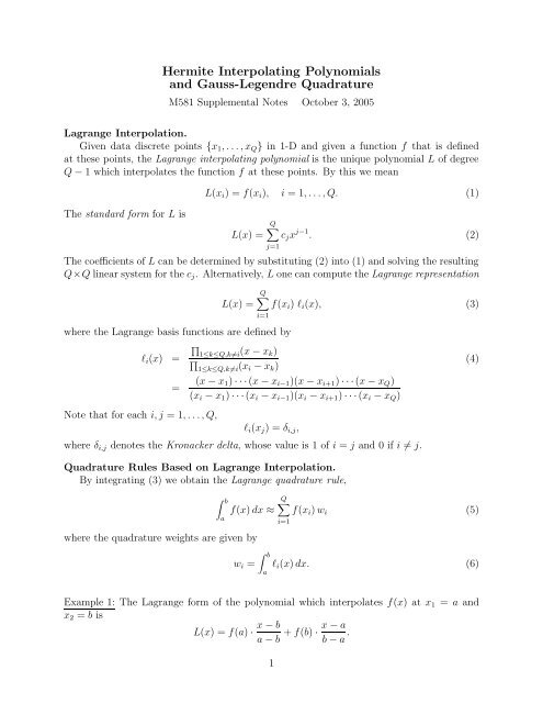
Hermite Interpolating Polynomials and Gauss-Legendre Quadrature

Hermite Interpolating Polynomials
and Gauss-Legendre Quadrature
M581 Supplemental Notes October 3, 2005
Lagrange Interpolation.
Given data discrete points {x1, . . . , xQ} in 1-D and given a function f that is defined
at these points, the Lagrange interpolating polynomial is the unique polynomial L of degree
Q − 1 which interpolates the function f at these points. By this we mean
The standard form for L is
L(xi) = f(xi), i = 1, . . . , Q. (1)
Q
L(x) = cjx
j=1
j−1 . (2)
The coefficients of L can be determined by substituting (2) into (1) and solving the resulting
Q×Q linear system for the cj. Alternatively, L one can compute the Lagrange representation
where the Lagrange basis functions are defined by
ℓi(x) =
1≤k≤Q,k=i(x − xk)
1≤k≤Q,k=i(xi − xk)
Note that for each i, j = 1, . . . , Q,
Q
L(x) = f(xi) ℓi(x), (3)
i=1
= (x − x1) · · · (x − xi−1)(x − xi+1) · · · (x − xQ)
(xi − x1) · · · (xi − xi−1)(xi − xi+1) · · · (xi − xQ)
ℓi(xj) = δi,j,
where δi,j denotes the Kronacker delta, whose value is 1 of i = j and 0 if i = j.
Quadrature Rules Based on Lagrange Interpolation.
By integrating (3) we obtain the Lagrange quadrature rule,
where the quadrature weights are given by
b
Q
f(x) dx ≈ f(xi) wi
a
i=1
wi =
b
a
(4)
(5)
ℓi(x) dx. (6)
Example 1: The Lagrange form of the polynomial which interpolates f(x) at x1 = a and
x2 = b is
x − b x − a
L(x) = f(a) · + f(b) ·
a − b b − a .
1

Integrating L(x) over the interval a ≤ x ≤ b yields the trapazoidal rule
b
a
f(x) dx ≈
b
b
f(a) (x − b) dx/(a − b) + f(b) (x − a) dx/(b − a)
a
a
= f(a) ·
b − a
2
+ f(b) · b − a
2 ,
Here Q = 2, the quadrature points are x1 = a, x2 = b, and the quadrature weights are
w1 = w2 = b−a
2 .
Error Analysis for Lagrange Quadrature.
If L(x) is the polynomial of degree Q − 1 which interpolates f(x) at {xi} Q
i=1 and if
f ∈ C Q [a, b], then it can be shown that the pointwise approximation error is given by
where
f(x) − L(x) = 1 d
Q!
Qf dxQ (ξx) π(x), for some ξx ∈ (a, b), (7)
Q
π(x) ≡ (x − xk) = (x − x1)(x − x2) · · · (x − xQ). (8)
k=1
By integrating (7) we obtain the quadrature error bounds
b
Q
f(x)dx − f(xq)wq
a
q=0
=
1
b
d
Q! a
Qf dxQ (ξx)
≤
π(x) dx
1
Q! max
d
a≤ξ≤b
Q ≤
f b
(ξ) |π(x)| dx
dxQ a
(9)
1
Q! max
d
a≤ξ≤b
Q
f
(ξ)
dxQ max
a≤x≤b |π(x)|
b
dx
a
≤ const (b − a) Q+1 . (10)
Defining the interval length h = b − a, we obtain O(h Q+1 ) accuracy. The quadrature rule is
exact (i.e., there is no quadrature error) for all polynomials of degree ≤ Q − 1 because the
Qth derivative of these polynomials vanishes.
Continuation of Example 1: For the trapazoidal rule, Q = 2, so the method is exact for
polynomials of degree ≤ 1 and the accuracy is O(h 3 ) provided the function being integrated
is twice continuously differentiable.
Exercise 1. Derive Simpson’s rule, which is based on interpolation at points a, (a + b)/2,
and b, and show that the accuracy is O(h 4 ), where h = b − a.
Hermite Interpolation.
Given a differentiable function f defined on discrete points {x1, . . . , xQ}, the Hermite
interpolating polynomial is the unique polynomial H of degree 2Q − 1 that interpolates f
and its derivative,
H(xi) = f(xi),
dH
dx (xi) = df
dx (xi), i = 1, . . . , Q. (11)
2

H(x) does have a standard representation which is analogous to eqn (2), but to derive
quadrature rules it is convenient to use the Hermite representation
where
Q
H(x) = f(xi) hi(x) +
Q
i=1
i=1
hi(x) =
1 − 2 dℓi
dx (xi)
(x − xi)
df
dx (xi) hi(x), (12)
ℓ 2 i (x) (13)
hi(x) = (x − xi) ℓ 2 i (x) (14)
with Lagrange basis functions ℓi defined as before in (4).
Exercise 2. Verify that for each i, j = 1, . . . , Q,
hi(xj) = δij,
hi(xj) = 0,
and hence, the interpolation conditions (11) hold.
Gauss-Legendre Quadrature.
By integrating (12) we obtain a Hermite quadrature rule
b
Q
b
f(x) dx ≈ f(xi) hi(x) dx +
a
i=1
a
wi
dhi
dx (xj) = 0, (15)
dhi
dx (xj) = δij, (16)
Q
i=1
df
dx (xi)
b
hi(x) dx
a
wi
. (17)
The key to obtaining a numerical integration scheme, called Gauss-Legendre quadrature,
which is exact for all polynomials of degree ≤ degree 2Q − 1 is to pick the quadrature points
to be (possibly transformed) roots of Legendre polynomials. This will cause the terms wi in
the second sum in (17) to vanish.
Let PQ denote the Qth Legendre polynomial. This has leading coefficient 1 and it is
orthogonal on the interval [−1, 1] to Legendre polynomials Pi of lower degree,
1
PQ(x) Pi(x) dx = 0, i = 1, . . . , Q − 1.
−1
Since any polynomial can be expressed as a linear combination of Legendre polynomials,
1
PQ(x)ρ(x) dx for any polynomial ρ of degree < Q. (18)
−1
From (14) one can factor
hi(x) = (x − xi)ℓi(x) ℓi(x) = π(x) × Cℓi(x), (19)
where π is the degree Q polynomial defined in (8) and C is some constant. Note that the
degree of ℓi is Q − 1. By selecting the xis to be the roots of the Qth Legendre polynomial
PQ, we obtain π(x) = PQ(x), and from (18) and (19) we obtain
wi =
1
−1
hi(x) dx = 0.
3

Consequently
where
1
Q
f(x) dx ≈ f(xi) wi
−1
i=1
wi =
1
−1
hi(x) dx
whenever the quadrature points xi are taken to be the roots of the Legendre polynomial of
degree Q.
Exercise 3. Obtain a corresponding quadrature rule for an arbitrary interval [a, b], by
deriving the linear transformation that maps [a, b] onto [−1, 1] and then applying the change
of variables formula for integrals. Provide explicit formulas for the quadrature points and
weights for [a, b] in terms of the quadrature points and weights for [−1, 1].
Error Analysis for Gauss-Legendre Quadrature.
If f ∈ C 2Q [a, b] and we select Gauss-Legendre quadrature points for interpolation, then
f(x) = H(x) + 1 d
(2Q)!
Qf dxQ (ξx) π 2 (x),
where H is the degree 2Q − 1 Hermite interpolating polynomial, ξx is some point in the
interval (a, b), and π is defined in (8). From the derivations above we obtain
b
a
f(x) dx =
=
b
a
Q
i=1
H(x) dx + 1
b d
(2Q)! a
Qf dxQ (ξx) π 2 (x) dx
f(xi) wi + O(h 2Q+1 ),
with h = b − a. The error term derivation follows as in the case of Lagrange quadrature
error.
The following table summarizes the first two Gaussian quadrature rules for the interval
[−1, 1].
Q = 1 Q = 2
w1 = 2 w1 = w2 = 1
x1 = 0 x1, x2 = ∓ 1
√ 3
3 nd order accuracy 5 th order accuracy
Exercise 4. Derive the Gaussian quadrature rules in the table above. Then give corresponding
rules (i.e., points and weights) for the interval [0, 1].
4