Hermite Interpolating Polynomials and Gauss-Legendre Quadrature

Consequently
where
1
Q
f(x) dx ≈ f(xi) wi
−1
i=1
wi =
1
−1
hi(x) dx
whenever the quadrature points xi are taken to be the roots of the Legendre polynomial of
degree Q.
Exercise 3. Obtain a corresponding quadrature rule for an arbitrary interval [a, b], by
deriving the linear transformation that maps [a, b] onto [−1, 1] and then applying the change
of variables formula for integrals. Provide explicit formulas for the quadrature points and
weights for [a, b] in terms of the quadrature points and weights for [−1, 1].
Error Analysis for Gauss-Legendre Quadrature.
If f ∈ C 2Q [a, b] and we select Gauss-Legendre quadrature points for interpolation, then
f(x) = H(x) + 1 d
(2Q)!
Qf dxQ (ξx) π 2 (x),
where H is the degree 2Q − 1 Hermite interpolating polynomial, ξx is some point in the
interval (a, b), and π is defined in (8). From the derivations above we obtain
b
a
f(x) dx =
=
b
a
Q
i=1
H(x) dx + 1
b d
(2Q)! a
Qf dxQ (ξx) π 2 (x) dx
f(xi) wi + O(h 2Q+1 ),
with h = b − a. The error term derivation follows as in the case of Lagrange quadrature
error.
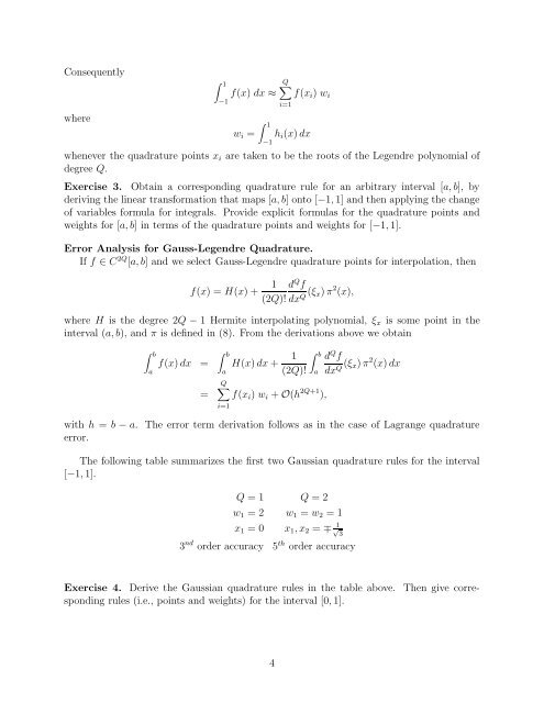
The following table summarizes the first two Gaussian quadrature rules for the interval
[−1, 1].
Q = 1 Q = 2
w1 = 2 w1 = w2 = 1
x1 = 0 x1, x2 = ∓ 1
√ 3
3 nd order accuracy 5 th order accuracy
Exercise 4. Derive the Gaussian quadrature rules in the table above. Then give corresponding
rules (i.e., points and weights) for the interval [0, 1].
4