CHAPTER 3 - Educators
CHAPTER 3 - Educators
CHAPTER 3 - Educators

You also want an ePaper? Increase the reach of your titles
YUMPU automatically turns print PDFs into web optimized ePapers that Google loves.
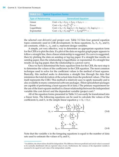
94 <strong>CHAPTER</strong> 3/COST-ESTIMATION TECHNIQUES<br />
TABLE 3-2 Typical Equation Forms<br />
Type of Relationship Generalized Equation<br />
Linear Cost = b0 + b1x1 + b2x2 + b3x3 +···<br />
Power Cost = b0 + b1x b11<br />
1 xb12<br />
2 +···<br />
Logarithmic Cost = b0 + b1 log(x1) + b2 log(x2) + b3 log(x3) +···<br />
Exponential Cost = b0 + b1 expb11x1 + b2 expb22x2 +···<br />
the selected cost driver(s) and project cost. Table 3-2 lists four general equation<br />
types commonly used in CER development. In these equations, b0, b1, b2, and b3<br />
are constants, while x1, x2, and x3 represent design variables.<br />
A simple, yet very effective, way to determine an appropriate equation form<br />
for the CER is to plot the data. If a plot of the data on regular graph paper appears to<br />
follow a straight line, then a linear relationship is suggested. If a curve is suggested,<br />
then try plotting the data on semilog or log-log paper. If a straight line results on<br />
semilog paper, then the relationship is logarithmic or exponential. If a straight line<br />
results on log-log paper, then the relationship is a power curve.<br />
Once we have determined the basic equation form for the CER, the next step is<br />
to determine the values of the coefficients in the CER equation. The most common<br />
technique used to solve for the coefficient values is the method of least squares.<br />
Basically, this method seeks to determine a straight line through the data that<br />
minimizes the total deviation of the actual data from the predicted values. (The line<br />
itself represents the CER.) This method is relatively easy to apply manually and is<br />
also available in many commercial software packages. (Most spreadsheet packages<br />
are capable of performing a least-squares fit of data.) The primary requirement for<br />
the use of the least-squares method is a linear relationship between the independent<br />
variable (the cost driver) and the dependent variable (project cost). ∗<br />
All of the equation forms presented in Table 3-2 can easily be transformed into<br />
a linear form. The following equations can be used to calculate the values of the<br />
coefficients b0 and b1 in the simple linear equation y = b0 + b1x:<br />
n<br />
<br />
n<br />
<br />
n<br />
<br />
n xiyi −<br />
b1 =<br />
i=1<br />
n<br />
i=1<br />
xi<br />
n<br />
x 2 i −<br />
<br />
n<br />
i=1<br />
n<br />
i=1<br />
n<br />
xi<br />
yi − b1 xi<br />
i=1 i=1<br />
i=1<br />
2 yi<br />
, (3-8)<br />
b0 =<br />
. (3-9)<br />
n<br />
Note that the variable n in the foregoing equations is equal to the number of data<br />
sets used to estimate the values of b0 and b1.<br />
∗ In addition, the observations should be independent. The difference between predicted and actual values is assumed<br />
to be normally distributed with an expected value of zero. Furthermore, the variance of the dependent variable is<br />
assumed to be equal for each value of the independent variable.