CHAPTER 3 - Educators

CHAPTER 3 

Cost-Estimation Techniques 

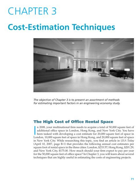
The objective of Chapter 3 is to present an assortment of methods 

for estimating important factors in an engineering economy study. 

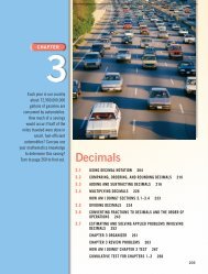
The High Cost of Office Rental Space 

In2008, your multinational firm needs to acquire a total of 50,000 square feet of 

additional office space in London, Hong Kong, and New York City. You have 

been tasked with developing a cost estimate for 20,000 square feet of space in 

London, 10,000 square feet of space in Hong Kong, and 20,000 square feet of space 

in New York City. While researching this topic, you find an article in USA Today 

(April 10, 2007, page B-1) that provides the following annual cost estimates per 

square foot of rental space in the three cities: London, $233.57; Hong Kong, $201.29; 

and New York City, $175.00. How much should your firm expect to pay per year 

for the 50,000 square feet of office space? In Chapter 3, you will learn about several 

techniques that are highly useful in estimating the costs of engineering projects. 

71

3.1 Introduction 

72 

Decisions, both great and small, depend in part on estimates. “Looking down the barrel” need 

not be an embarrassment for the engineer if newer techniques, professional staffing, and a 

greater awareness are assigned to the engineering cost estimating function. 

—Phillip F. Ostwald (1992) 

In Chapter 1, we described the engineering economic analysis procedure in terms 

of seven steps. In this chapter, we address Step 3, development of the outcomes 

and cash flows for each alternative. Because engineering economy studies deal 

with outcomes that extend into the future, estimating the future cash flows for 

feasible alternatives is a critical step in the analysis procedure. Often, the most 

difficult, expensive, and time-consuming part of an engineering economy study 

is the estimation of costs, revenues, useful lives, residual values, and other data 

pertaining to the alternatives being analyzed. A decision based on the analysis is 

economically sound only to the extent that these cost and revenue estimates are 

representative of what subsequently will occur. In this chapter, we introduce the 

role of cost estimating in engineering practice. Definitions and examples of important 

cost concepts were provided in Chapter 2. 

Whenever an engineering economic analysis is performed for a major capital 

investment, the cost-estimating effort for that analysis should be an integral part of 

a comprehensive planning and design process requiring the active participation of 

not only engineering designers but also personnel from marketing, manufacturing, 

finance, and top management. Results of cost estimating are used for a variety of 

purposes, including the following: 

1. Providing information used in setting a selling price for quoting, bidding, or 

evaluating contracts 

2. Determining whether a proposed product can be made and distributed at a 

profit (for simplicity, price = cost + profit) 

3. Evaluating how much capital can be justified for process changes or other 

improvements 

4. Establishing benchmarks for productivity improvement programs 

There are two fundamental approaches to cost estimating: the “top-down” 

approach and the “bottom-up” approach. The top-down approach basically uses 

historical data from similar engineering projects to estimate the costs, revenues, and 

other data for the current project by modifying these data for changes in inflation 

or deflation, activity level, weight, energy consumption, size, and other factors. 

This approach is best used early in the estimating process when alternatives are 

still being developed and refined. 

The bottom-up approach is a more detailed method of cost estimating. This 

method breaks down a project into small, manageable units and estimates their 

economic consequences. These smaller unit costs are added together with other 

types of costs to obtain an overall cost estimate. This approach usually works best 

when the detail concerning the desired output (a product or a service) has been 

defined and clarified.

EXAMPLE 3-1 Estimating the Cost of a College Degree 

SECTION 3.1/INTRODUCTION 73 

A simple example of cost estimating is to forecast the expense of getting a 

Bachelor of Science (B.S.) from the university you are attending. In our solution, 

we outline the two basic approaches just discussed for estimating these costs. 

Solution 

A top-down approach would take the published cost of a four-year degree at 

the same (or a similar) university and adjust it for inflation and extraordinary 

items that an incoming student might encounter, such as fraternity/sorority 

membership, scholarships, and tutoring. For example, suppose that the published 

cost of attending your university is $15,750 for the current year. This 

figure is anticipated to increase at the rate of 6% per year and includes fulltime 

tuition and fees, university housing, and a weekly meal plan. Not 

included are the costs of books, supplies, and other personal expenses. For 

our initial estimate, these “other” expenses are assumed to remain constant at 

$5,000 per year. 

The total estimated cost for four years can now be computed. We simply 

need to adjust the published cost for inflation each year and add in the cost of 

“other” expenses. 

Tuition, Fees, “Other” Total Estimated 

Year Room and Board Expenses Cost for Year 

1 $15,750 × 1.06 = $16,695 $5,000 $21,695 

2 16,695 × 1.06 = 17,697 5,000 22,697 

3 17,697 × 1.06 = 18,759 5,000 23,759 

4 18,759 × 1.06 = 19,885 5,000 24,885 

Grand Total $93,036 

In contrast with the top-down approach, a bottom-up approach to the same 

cost estimate would be to first break down anticipated expenses into the typical 

categories shown in Figure 3-1 for each of the four years at the university. 

Tuition and fees can be estimated fairly accurately in each year, as can books and 

supplies. For example, suppose that the average cost of a college textbook is $100. 

You can estimate your annual textbook cost by simply multiplying the average 

cost per book by the number of courses you plan to take. Assume that you 

plan on taking five courses each semester during the first year. Your estimated 

textbook costs would be 

5 courses 

semester 

 

(2 semesters) 

1 book 

course 

 

$100 

= $1,000. 

book 

The other two categories, living expenses and transportation, are probably 

more dependent on your lifestyle. For example, whether you own and operate 

an automobile and live in a “high-end” apartment off-campus can dramatically 

affect the estimated expenses during your college years.

74 CHAPTER 3/COST-ESTIMATION TECHNIQUES 

Tuition and 

Fees 

2009 

2008 

Tuition 

Activities fees 

Memberships 

Medical insurance 

Lab fees 

2011 

2010 

Sum over Four Years to Obtain Total Cost 

of a B.S. at Your University 

Books and 

Supplies 

Books 

Duplication 

Supplies 

Computer rental 

Software 

Living 

Expenses 

Rent 

Food 

Clothing 

Recreation 

Utilities 

Figure 3-1 Bottom-Up Approach to Determining the Cost 

of a College Education 

3.2 An Integrated Approach 

Transportation 

Fuel 

Maintenance on car 

Insurance 

Traffic tickets 

An integrated approach to developing the net cash flows for feasible project 

alternatives is shown in Figure 3-2. This integrated approach includes three basic 

components: 

1. Work breakdown structure (WBS) This is a technique for explicitly defining, 

at successive levels of detail, the work elements of a project and their 

interrelationships (sometimes called a work element structure). 

2. Cost and revenue structure (classification) Delineation of the cost and revenue 

categories and elements is made for estimates of cash flows at each level of the 

WBS. 

3. Estimating techniques (models) Selected mathematical models are used to 

estimate the future costs and revenues during the analysis period. 

These three basic components, together with integrating procedural steps, provide 

an organized approach for developing the cash flows for the alternatives.

Cost and 

revenue 

database 

Determine 

WBS level(s) for 

estimating 

Define 

Cash flow perspective 

Estimating baseline 

Study (analysis) period 

Yes 

Stop 

Last 

alternative 

? 

Develop 

cash flow for 

alternative 

Describe a 

feasible alternative 

using project WBS 

Describe project in 

work breakdown 

structure (WBS) form 

No 

(Basic Component 1) 

Estimating 

techniques 

(models) 

Delineate cost 

and revenue 

categories 

and elements 



Figure 3-2 Integrated Approach for Developing the Cash Flows for Alternatives 

75


As shown in Figure 3-2, the integrated approach begins with a description 

of the project in terms of a WBS. WBS is used to describe the project and each 

alternative’s unique characteristics in terms of design, labor, material requirements, 

and so on. Then these variations in design, resource requirements, and other 

characteristics are reflected in the estimated future costs and revenues (net cash 

flow) for that alternative. 

To estimate future costs and revenues for an alternative, the perspective 

(viewpoint) of the cash flow must be established and an estimating baseline and 

analysis period defined. Normally, cash flows are developed from the owner’s 

viewpoint. The net cash flow for an alternative represents what is estimated to 

happen to future revenues and costs from the perspective being used. Therefore, the 

estimated changes in revenues and costs associated with an alternative have to be 

relative to a baseline that is consistently used for all the alternatives being compared. 

3.2.1 The Work Breakdown Structure (WBS) 

The first basic component in an integrated approach to developing cash flows 

is the work breakdown structure (WBS). The WBS is a basic tool in project 

management and is a vital aid in an engineering economy study. The WBS serves 

as a framework for defining all project work elements and their interrelationships, 

collecting and organizing information, developing relevant cost and revenue data, 

and integrating project management activities. 

Figure 3-3 shows a diagram of a typical four-level WBS. It is developed from 

the top (project level) down in successive levels of detail. The project is divided 

into its major work elements (Level 2). These major elements are then divided to 

develop Level 3, and so on. For example, an automobile (first level of the WBS) can 

be divided into second-level components (or work elements) such as the chassis, 

drive train, and electrical system. Then each second-level component of the WBS 

can be subdivided further into third-level elements. The drive train, for example, 

can be subdivided into third-level components such as the engine, differential, and 

transmission. This process is continued until the desired detail in the definition 

and description of the project or system is achieved. 

Different numbering schemes may be used. The objectives of numbering are to 

indicate the interrelationships of the work elements in the hierarchy. The scheme 

illustrated in Figure 3-3 is an alphanumeric format. Another scheme often used is all 

numeric—Level 1: 1-0; Level 2: 1-1, 1-2, 1-3; Level 3: 1-1-1, 1-1-2, 1-2-1, 1-2-2, 1-3-1, 

1-3-2; and so on (i.e., similar to the organization of this book). Usually, the level is 

equal (except for Level 1) to the number of characters indicating the work element. 

Other characteristics of a project WBS are as follows: 

1. Both functional (e.g., planning) and physical (e.g., foundation) work elements 

are included in it: 

(a) Typical functional work elements are logistical support, project 

management, marketing, engineering, and systems integration. 

(b) Physical work elements are the parts that make up a structure, product, 

piece of equipment, or similar item; they require labor, materials, and other 

resources to produce or construct.

Level 4 

Level 3 

A 1 A 

Level 2 

A 1 

A 1 B 

A 1 A 1 A 1 B 2 

Figure 3-3 The WBS Diagram 

Level 1 

A 0 

SECTION 3.2/AN INTEGRATED APPROACH 77 

A 2 A 3 

2. The content and resource requirements for a work element are the sum of the 

activities and resources of related subelements below it. 

3. A project WBS usually includes recurring (e.g., maintenance) and nonrecurring 

(e.g., initial construction) work elements. 

EXAMPLE 3-2 A WBS for a Construction Project 

You have been appointed by your company to manage a project involving 

construction of a small commercial building with two floors of 15,000 gross 

square feet each. The ground floor is planned for small retail shops, and 

the second floor is planned for offices. Develop the first three levels of a 

representative WBS adequate for all project efforts from the time the decision 

was made to proceed with the design and construction of the building until 

initial occupancy is completed. 

Solution 

There would be variations in the WBSs developed by different individuals for a 

commercial building. A representative three-level WBS is shown in Figure 3-4. 

Level 1 is the total project. At Level 2, the project is divided into seven major 

physical work elements and three major functional work elements. Then each 

of these major elements is divided into subelements as required (Level 3). The 

numbering scheme used in this example is all numeric.


78 

Commercial 

Building Project 

1-0 

LEVEL 

1 

Roof 

Interior 

Exterior 

1-4 

1-3 

1-2 

Site Work 

and Foundation 

1-1 

2 

1-4-1 

Framing 

1-4-2 

Sheathing 

1-3-1 

Framing 

1-3-2 

Flooring/Stairways 

1-2-1 

Framing 

1-1-1 

Site Grading 

1-2-2 

Siding 

1-1-2 

Excavation 

1-4-3 

Roofing 

1-3-3 

Walls/Ceilings 

1-2-3 

Windows 

1-1-3 

Sidewalks/Parking 

3 

1-3-4 

Doors 

1-3-5 

Special Additions 

1-2-4 

Entrances 

1-1-4 

Footing/Foundation 

1-2-5 

Insulation 

1-1-5 

Floor Slab 

Sales 

Project 

Management 

1-8 

Real 

Estate 

1-10 

1-7 

Mechanical 

Systems 

1-6 

Electrical 

Systems 

1-5 

1-10-1 

Leasing/Asset Sales 

1-10-2 

Admin. Support 

Arch/Engr. 

Services 

1-9 

1-9-1 

Design 

1-9-2 

Cost Estimating 

2 

1-8-1 

Admin. Support 

1-6-1 

Heating/Cooling 

1-5-1 

Service Delivery 

1-8-2 

Technical Mgt. 

1-6-2 

Hot Water 

1-5-2 

Devices 

3 

1-10-3 

Legal 

1-9-3 

Consulting 

1-8-3 

Legal 

1-6-3 

Lavatories 

1-5-3 

Lighting 

Figure 3-4 WBS (Three Levels) for Commercial Building Project in Example 3-2

3.2.2 The Cost and Revenue Structure 


The second basic component of the integrated approach for developing cash 

flows (Figure 3-2) is the cost and revenue structure. This structure is used to 

identify and categorize the costs and revenues that need to be included in 

the analysis. Detailed data are developed and organized within this structure 

for use with the estimating techniques of Section 3.3 to prepare the cash-flow 

estimates. 

The life-cycle concept and the WBS are important aids in developing the cost 

and revenue structure for a project. The life cycle defines a maximum time period 

and establishes a range of cost and revenue elements that need to be considered 

in developing cash flows. The WBS focuses the analyst’s effort on the specific 

functional and physical work elements of a project and on its related costs 

and revenue. 

Perhaps the most serious source of errors in developing cash flows is overlooking 

important categories of costs and revenues. The cost and revenue structure, 

prepared in tabular or checklist form, is a good means of preventing such 

oversights. Technical familiarity with the project is essential in ensuring the 

completeness of the structure, as are using the life-cycle concept and the WBS 

in its preparation. 

The following is a brief listing of some categories of costs and revenues that 

are typically needed in an engineering economy study: 

1. Capital investment (fixed and working) 

2. Labor costs 

3. Material costs 

4. Maintenance costs 

5. Property taxes and insurance 

6. Overhead costs 

7. Disposal costs 

8. Revenues 

9. Quality (and scrap) costs 

10. Market (or salvage) values 

3.2.3 Estimating Techniques (Models) 

The third basic component of the integrated approach (Figure 3-2) involves 

estimating techniques (models). These techniques, together with the detailed cost 

and revenue data, are used to develop individual cash-flow estimates and the 

overall net cash-flow for each alternative.


The purpose of estimating is to develop cash-flow projections—not to produce 

exact data about the future, which is virtually impossible. Neither a preliminary 

estimate nor a final estimate is expected to be exact; rather, it should adequately 

suit the need at a reasonable cost and is often presented as a range of numbers. 

Cost and revenue estimates can be classified according to detail, accuracy, and 

their intended use as follows: 

1. Order-of-magnitude estimates: used in the planning and initial evaluation stage 

of a project. 

2. Semidetailed, or budget, estimates: used in the preliminary or conceptual 

design stage of a project. 

3. Definitive (detailed) estimates: used in the detailed engineering/construction 

stage of a project. 

Order-of-magnitude estimates are used in selecting the feasible alternatives for the 

study. They typically provide accuracy in the range of ±30 to 50% and are developed 

through semiformal means such as conferences, questionnaires, and generalized 

equations applied at Level 1 or 2 of the WBS. 

Budget (semidetailed) estimates are compiled to support the preliminary 

design effort and decision making during this project period. Their accuracy usually 

lies in the range of ±15%. These estimates differ in the fineness of cost and revenue 

breakdowns and the amount of effort spent on the estimate. Estimating equations 

applied at Levels 2 and 3 of the WBS are normally used. 

Detailed estimates are used as the basis for bids and to make detailed design 

decisions. Their accuracy is ±5%. They are made from specifications, drawings, 

site surveys, vendor quotations, and in-house historical records and are usually 

done at Level 3 and successive levels in the WBS. 

Thus, it is apparent that a cost or revenue estimate can vary from a “back of the 

envelope” calculation by an expert to a very detailed and accurate prediction of 

the future prepared by a project team. The level of detail and accuracy of estimates 

should depend on the following: 

1. Time and effort available as justified by the importance of the study 

2. Difficulty of estimating the items in question 

3. Methods or techniques employed 

4. Qualifications of the estimator(s) 

5. Sensitivity of study results to particular factor estimates 

As estimates become more detailed, accuracy typically improves, but the cost of 

making the estimate increases dramatically. This general relationship is shown 

in Figure 3-5 and illustrates the idea that cost and revenue estimates should be 

prepared with full recognition of how accurate a particular study requires them 

to be.

Figure 3-5 

Accuracy of Cost 

and Revenue 

Estimates versus 

the Cost of 

Making Them 

Cost of Estimate 

as a Percentage of Project Cost 

10 

5 

Detailed Estimates 


Levels 25 

3–4 

in WBS 

Accuracy (%) 

Order-of-Magnitude 

Estimates 

Levels 

1–2 

in WBS 

3.2.3.1 Sources of Estimating Data The information sources useful in cost 

and revenue estimating are too numerous to list completely. The following four 

major sources of information are listed roughly in order of importance: 

1. Accounting records. Accounting records are a prime source of information 

for economic analyses; however, they are often not suitable for direct, 

unadjusted use. 

A brief discussion of the accounting process and information was given 

in Appendix 2-A. In its most basic sense, accounting consists of a series of 

procedures for keeping a detailed record of monetary transactions between 

established categories of assets. Accounting records are a good source of 

historical data but have some limitations when used in making prospective 

estimates for engineering economic analyses. Moreover, accounting records 

rarely contain direct statements of incremental costs or opportunity costs, both 

of which are essential in most engineering economic analyses. Incremental 

costs are decision specific for one-of-a-kind investments and are unlikely to 

be available from the accounting system. 

2. Other sources within the firm. The typical firm has a number of people and 

records that may be excellent sources of estimating information. Examples 

of functions within firms that keep records useful to economic analyses are 

engineering, sales, production, quality, purchasing, and personnel. 

3. Sources outside the firm. There are numerous sources outside the firm that 

can provide helpful information. The main problem is in determining those 

that are most beneficial for particular needs. The following is a listing of some 

commonly used outside sources: 

(a) Published information. Technical directories, buyer indexes, U.S. government 

publications, reference books, and trade journals offer a wealth of information. 

For instance, Standard and Poor’s Industry Surveys gives monthly 

information regarding key industries. The Statistical Abstract of the United 

States is a remarkably comprehensive source of cost indexes and data. The 

Bureau of Labor Statistics publishes many periodicals that are good sources 

of labor costs, such as the Monthly Labor Review, Employment and Earnings, 

50


Current Wage Developments, Handbook of Labor Statistics, and the Chartbook 

on Wages, Prices and Productivity. 

(b) Personal contacts are excellent potential sources. Vendors, salespeople, 

professional acquaintances, customers, banks, government agencies, 

chambers of commerce, and even competitors are often willing to furnish 

needed information on the basis of a serious and tactful request. 

4. Research and development (R&D). If the information is not published and 

cannot be obtained by consulting someone, the only alternative may be to 

undertake R&D to generate it. Classic examples are developing a pilot plant 

and undertaking a test market program. 

The Internet can also be a source of cost-estimating data, though you should assure 

yourself that the information is from a reputable source. The following Web sites 

may be useful to you both professionally and personally. 

www.enr.com Engineering News-Record Construction and labor costs 

www.kbb.com Kelley Blue Book Automobile pricing 

www.factsonfuel.com American Petroleum Institute Fuel costs 

3.2.3.2 How Estimates Are Accomplished Estimates can be prepared in a 

number of ways, such as the following examples: 

1. A conference of various people who are thought to have good information or 

bases for estimating the quantity in question. A special version of this is the 

Delphi method, which involves cycles of questioning and feedback in which the 

opinions of individual participants are kept anonymous. 

2. Comparison with similar situations or designs about which there is more 

information and from which estimates for the alternatives under consideration 

can be extrapolated. This is sometimes called estimating by analogy. The 

comparison method may be used to approximate the cost of a design or product 

that is new. This is done by taking the cost of a more complex design for a similar 

item as an upper bound and the cost of a less complex item of similar design 

as a lower bound. The resulting approximation may not be very accurate, but 

the comparison method does have the virtue of setting bounds that might be 

useful for decision making. 

3. Using quantitative techniques, which do not always have standardized names. 

Some selected techniques, with the names used being generally suggestive of 

the approaches, are discussed in the next section. 

3.3 Selected Estimating Techniques (Models) 

The estimating models discussed in this section are applicable for order-ofmagnitude 

estimates and for many semidetailed or budget estimates. They are 

useful in the initial selection of feasible alternatives for further analysis and in the 

conceptual or preliminary design phase of a project. Sometimes, these models can 

be used in the detailed design phase of a project.

3.3.1 Indexes 

SECTION 3.3/SELECTED ESTIMATING TECHNIQUES (MODELS) 83 

Costs and prices∗ vary with time for a number of reasons, including (1) 

technological advances, (2) availability of labor and materials, and (3) inflation. An 

index is a dimensionless number that indicates how a cost or a price has changed 

with time (typically escalated) with respect to a base year. Indexes provide a 

convenient means for developing present and future cost and price estimates from 

historical data. An estimate of the cost or selling price of an item in year n can be 

obtained by multiplying the cost or price of the item at an earlier point in time 

(year k) by the ratio of the index value in year n (Īn) to the index value in year k 

(Īk); † that is, 

 

Īn 

, (3-1) 

Cn = Ck 

where k = reference year (e.g., 2000) for which cost or price of item is known; 

n = year for which cost or price is to be estimated (n > k); 

Cn = estimated cost or price of item in year n; 

Ck = cost or price of item in reference year k. 

Equation (3-1) is sometimes referred to as the ratio technique of updating costs and 

prices. Use of this technique allows the cost or potential selling price of an item 

to be taken from historical data with a specified base year and updated with an 

index. This concept can be applied at the lower levels of a WBS to estimate the cost 

of equipment, materials, and labor, as well as at the top level of a WBS to estimate 

the total project cost of a new facility, bridge, and so on. 

EXAMPLE 3-3 Indexing the Cost of a New Boiler 

A certain index for the cost of purchasing and installing utility boilers is keyed to 

1988, where its baseline value was arbitrarily set at 100. Company XYZ installed 

a 50,000-lb/hour boiler for $525,000 in 2000 when the index had a value of 468. 

This same company must install another boiler of the same size in 2007. The 

index in 2007 is 542. What is the approximate cost of the new boiler? 

Solution 

In this example, n is 2007 and k is 2000. From Equation (3-1), an approximate 

cost of the boiler in 2007 is 

C2007 = $525,000(542/468) = $608,013. 

Indexes can be created for a single item or for multiple items. For a single item, 

the index value is simply the ratio of the cost of the item in the current year to the 

cost of the same item in the reference year, multiplied by the reference year factor 

∗ The terms cost and price are often used together. The cost of a product or service is the total of the resources, direct 

and indirect, required to produce it. The price is the value of the good or service in the marketplace. In general, price 

is equal to cost plus a profit. 

† In this section only, k is used to denote the reference year. 

Īk


(typically, 100). A composite index is created by averaging the ratios of selected 

item costs in a particular year to the cost of the same items in a reference year. 

The developer of an index can assign different weights to the items in the index 

according to their contribution to total cost. For example, a general weighted index 

is given by 

Īn = W1(Cn1/Ck1) + W2(Cn2/Ck2) +···+WM(CnM/CkM) 

W1 + W2 +···+WM 

where M = total number of items in the index (1 ≤ m ≤ M); 

Cnm = unit cost (or price) of the mth item in year n; 

Ckm = unit cost (or price) of the mth item in year k; 

Wm = weight assigned to the mth item; 

Īk = composite index value in year k. 

× Īk, (3-2) 

The weights W1, W2, ..., WM can sum to any positive number, but typically sum 

to 1.00 or 100. Almost any combination of labor, material, products, services, and 

so on can be used for a composite cost or price index. 

EXAMPLE 3-4 Weighted Index for Gasoline Cost 

Based on the following data, develop a weighted index for the price of a gallon 

of gasoline in 2006, when 1992 is the reference year having an index value 

of 99.2. The weight placed on regular unleaded gasoline is three times that of 

either premium or unleaded plus, because roughly three times as much regular 

unleaded is sold compared with premium or unleaded plus. 

Price (Cents/Gal) in Year 

1992 1996 2006 

Premium 114 138 240 

Unleaded plus 103 127 230 

Regular unleaded 93 117 221 

Solution 

In this example, k is 1992 and n is 2006. From Equation (3-2), the value of Ī2006 is 

(1)(240/114) + (1)(230/103) + (3)(221/93) 

× 99.2 = 227.5. 

1 + 1 + 3 

Now, if the index in 2008, for example, is estimated to be 253, it is a simple matter 

to determine the corresponding 2008 prices of gasoline from Ī2006 = 227.5: 

 

253 

Premium: 240 cents/gal = 267 cents/gal, 

227.5

SECTION 3.3/SELECTED ESTIMATING TECHNIQUES (MODELS) 85 

 

253 

Unleaded plus: 230 cents/gal = 256 cents/gal, 

227.5 

 

253 

Regular unleaded: 221 cents/gal = 246 cents/gal. 

227.5 

Many indexes are periodically published, including the Engineering News 

Record Construction Index (www.enr.com), which incorporates labor and material 

costs and the Marshall and Stevens cost index. 

3.3.2 Unit Technique 

The unit technique involves using a per unit factor that can be estimated effectively. 

Examples are as follows: 

1. Capital cost of plant per kilowatt of capacity 

2. Revenue per mile 

3. Capital cost per installed telephone 

4. Revenue per customer served 

5. Temperature loss per 1,000 feet of steam pipe 

6. Operating cost per mile 

7. Construction cost per square foot 

Such factors, when multiplied by the appropriate unit, give a total estimate of cost, 

savings, or revenue. 

As a simple example, suppose that we need a preliminary estimate of the 

cost of a particular house. Using a unit factor of, say, $95 per square foot and 

knowing that the house is approximately 2,000 square feet, we estimate its cost to 

be $95 × 2,000 = $190,000. 

While the unit technique is very useful for preliminary estimating purposes, 

such average values can be misleading. In general, more detailed methods will 

result in greater estimation accuracy. 

3.3.3 Factor Technique 

The factor technique is an extension of the unit method in which we sum the product 

of several quantities or components and add these to any components estimated 

directly. That is, 

C = 

Cd + 

fmUm, (3-3) 

d 

m


where C = cost being estimated; 

Cd = cost of the selected component d that is estimated directly; 

fm = cost per unit of component m; 

Um = number of units of component m. 

As a simple example, suppose that we need a slightly refined estimate of the 

cost of a house consisting of 2,000 square feet, two porches, and a garage. 

Using a unit factor of $85 per square foot, $10,000 per porch, and $8,000 per 

garage for the two directly estimated components, we can calculate the total 

estimate as 

($10,000 × 2) + $8,000 + ($85 × 2,000) = $198,000. 

We can also answer the question posed at the beginning of the chapter (page 71) 

using the factor technique. The rental expense per year will be approximately 

20,000×$233.57 in London plus 10,000×$201.29 in Hong Kong plus 20,000×$175.00 

in New York City. The total expense will be $10,184,300 per year for the additional 

office space. 

The factor technique is particularly useful when the complexity of the 

estimating situation does not require a WBS, but several different parts are involved. 

Example 3-5 and the product cost-estimating example to be presented in Section 

3.5.1 further illustrate this technique. 

EXAMPLE 3-5 Analysis of Building Space Cost Estimates 

The detailed design of the commercial building described in Example 3-2 affects 

the utilization of the gross square feet (and, thus, the net rentable space) 

available on each floor. Also, the size and location of the parking lot and the 

prime road frontage available along the property may offer some additional 

revenue sources. As project manager, analyze the potential revenue impacts of 

the following considerations. 

The first floor of the building has 15,000 gross square feet of retail 

space, and the second floor has the same amount planned for office use. 

Based on discussions with the sales staff, develop the following additional 

information: 

(a) The retail space should be designed for two different uses—60% for a 

restaurant operation (utilization = 79%, yearly rent = $23/sq.ft.) and 40% 

for a retail clothing store (utilization = 83%, yearly rent = $18/sq.ft.). 

(b) There is a high probability that all the office space on the second floor will 

be leased to one client (utilization = 89%, yearly rent = $14/sq.ft.). 

(c) An estimated 20 parking spaces can be rented on a long-term basis to two 

existing businesses that adjoin the property. Also, one spot along the road 

frontage can be leased to a sign company, for erection of a billboard, without 

impairing the primary use of the property.

Solution 

SECTION 3.4/PARAMETRIC COST ESTIMATING 87 

Based on this information, you estimate annual project revenue ( ˆR) as 

ˆR = W(r1)(12) + ϒ(r2)(12) + 

3 

Sj(uj)(dj), 

where W = number of parking spaces; 

ϒ = number of billboards; 

r1 = rate per month per parking space = $22; 

r2 = rate per month per billboard = $65; 

j = index of type of building space use; 

Sj = space (gross square feet) being used for purpose j; 

uj = space j utilization factor (% net rentable); 

dj = rate per (rentable) square foot per year of building space used 

for purpose j. 

Then, 

ˆR =[20($22)(12) + 1($65)(12)]+[9,000(0.79)($23) 

+ 6,000(0.83)($18) + 15,000(0.89)($14)] 

ˆR = $6,060 + $440,070 = $446,130. 

A breakdown of the annual estimated project revenue shows that 

j=1 

1.4% is from miscellaneous revenue sources; 

98.6% is from leased building space. 

From a detailed design perspective, changes in annual project revenue due 

to changes in building space utilization factors can be easily calculated. For 

example, an average 1% improvement in the ratio of rentable space to gross 

square feet would change the annual revenue ( ˆR) as follows: 

ˆR = 

3 

Sj(uj + 0.01)(dj) − ($446,130 − $6,060) 

j=1 

3.4 Parametric Cost Estimating 

= $445,320 − $440,070 

= $5,250 per year. 

Parametric cost estimating is the use of historical cost data and statistical techniques 

to predict future costs. Statistical techniques are used to develop cost estimating 

relationships (CERs) that tie the cost or price of an item (e.g., a product, good,


TABLE 3-1 Examples of Cost Drivers Used in Parametric Cost Estimates 

Product Cost Driver (Independent Variable) 

Construction Floor space, roof surface area, wall surface area 

Trucks Empty weight, gross weight, horsepower 

Passenger car Curb weight, wheel base, passenger space, horsepower 

Turbine engine Maximum thrust, cruise thrust, specific fuel consumption 

Reciprocating engine Piston displacement, compression ratio, horsepower 

Aircraft Empty weight, speed, wing area 

Electrical power plants KiloWatts 

Motors Horsepower 

Software Number of lines of code 

service, or activity) to one or more independent variables (i.e., cost drivers). Recall 

from Chapter 2 that cost drivers are design variables that account for a large 

portion of total cost behavior. Table 3-1 lists a variety of items and associated cost 

drivers. The unit technique described in the previous section is a simple example 

of parametric cost estimating. 

Parametric models are used in the early design stages to get an idea of 

how much the product (or project) will cost, on the basis of a few physical 

attributes (such as weight, volume, and power). The output of the parametric 

models (an estimated cost) is used to gauge the impact of design decisions on the 

total cost. 

Various statistical and other mathematical techniques are used to develop 

the CERs. For example, simple linear regression and multiple linear regression 

models, which are standard statistical methods for estimating the value of 

a dependent variable (the unknown quantity) as a function of one or more 

independent variables, are often used to develop estimating relationships. This 

section describes two commonly used estimating relationships, the power-sizing 

technique and the learning curve, followed by an overview of the procedure used 

to develop CERs. 

3.4.1 Power-Sizing Technique 

The power-sizing technique, which is sometimes referred to as an exponential model, 

is frequently used for developing capital investment estimates for industrial plants 

and equipment. This CER recognizes that cost varies as some power of the change 

in capacity or size. That is, 

CA 

CB 

= 

SA 

CA = CB 

X 

, 

SB 

 

SA 

SB 

X 

, (3-4)

where CA = cost for plant A 

CB = cost for plant B 

SA = size of plant A 

SB = size of plant B 


 

(both in $ as of the point in 

time for which the estimate is 

desired); 

 

(both in same physical units); 

X = cost-capacity factor to reflect economies of scale. ∗ 

The value of the cost-capacity factor will depend on the type of plant or equipment 

being estimated. For example, X = 0.68 for nuclear generating plants and 0.79 

for fossil-fuel generating plants. Note that X < 1 indicates decreasing economies 

of scale (each additional unit of capacity costs less than the previous unit), X > 1 † 

indicates increasing economies of scale (each additional unit of capacity costs more 

than the previous unit), and X = 1 indicates a linear cost relationship with size. 

EXAMPLE 3-6 Power-Sizing Model for Cost Estimating 

Suppose that an aircraft manufacturer desires to make a preliminary estimate of 

the cost of building a 600-MW fossil-fuel plant for the assembly of its new longdistance 

aircraft. It is known that a 200-MW plant cost $100 million 20 years ago 

when the approximate cost index was 400, and that cost index is now 1,200. The 

cost-capacity factor for a fossil-fuel power plant is 0.79. 

Solution 

Before using the power-sizing model to estimate the cost of the 600-MW plant 

(CA), we must first use the cost index information to update the known cost of 

the 200-MW plant 20 years ago to a current cost. Using Equation (3-1), we find 

that the current cost of a 200-MW plant is 

 

1,200 

CB = $100 million = $300 million. 

400 

So, using Equation (3-4), we obtain the following estimate for the 600-MW plant: 

0.79 600-MW 

CA = $300 million 

200-MW 

CA = $300 million × 2.38 = $714 million. 

Note that Equation (3-4) can be used to estimate the cost of a larger plant (as 

in Example 3-6) or the cost of a smaller plant. For example, suppose we need to 

estimate the cost of building a 100-MW plant. Using Equation (3-4) and the data 

∗ This may be calculated or estimated from experience by using statistical techniques. For typical factors, see 

W. R. Park, Cost Engineering Analysis (New York: John Wiley & Sons, 1973), 137. 

† Precious gems are all example to increasing economies of scale. For example, a one-carat diamond typically costs 

more than four quarter-carat diamonds.


for the 200-MW plant in Example 3-6, we find that the current cost of a 100-MW 

plant is 

CA = $300 million 

0.79 100 MW 

200 MW 

CA = $300 million × 0.58 = $174 million. 

3.4.2 Learning and Improvement 

A learning curve is a mathematical model that explains the phenomenon of 

increased worker efficiency and improved organizational performance with 

repetitive production of a good or service. The learning curve is sometimes 

called an experience curve or a manufacturing progress function; fundamentally, it 

is an estimating relationship. The learning (improvement) curve effect was first 

observed in the aircraft and aerospace industries with respect to labor hours 

per unit. However, it applies in many different situations. For example, the 

learning curve effect can be used in estimating the professional hours expended 

by an engineering staff to accomplish successive detailed designs within a family 

of products, as well as in estimating the labor hours required to assemble 

automobiles. 

The basic concept of learning curves is that some input resources (e.g., 

energy costs, labor hours, material costs, engineering hours) decrease, on a peroutput-unit 

basis, as the number of units produced increases. Most learning curves 

are based on the assumption that a constant percentage reduction occurs in, say, 

labor hours, as the number of units produced is doubled. For example, if 100 labor 

hours are required to produce the first output unit and a 90% learning curve is 

assumed, then 100(0.9) = 90 labor hours would be required to produce the second 

unit. Similarly, 100(0.9) 2 = 81 labor hours would be needed to produce the fourth 

unit, 100(0.9) 3 = 72.9 hours to produce the eighth unit, and so on. Therefore, a 90% 

learning curve results in a 10% reduction in labor hours each time the production 

quantity is doubled. 

Equation (3-5) can be used to compute resource requirements assuming a 

constant percentage reduction in input resources each time the output quantity 

is doubled. 

Zu = K(u n ), (3-5) 

where u = the output unit number; 

Zu = the number of input resource units needed to produce output unit u; 

K = the number of input resource units needed to produce the first 

output unit; 

s = the learning curve slope parameter expressed as a decimal 

(s = 0.9 for a 90% learning curve); 

log s 

n = = the learning curve exponent. 

log 2

EXAMPLE 3-7 Learning Curve for a Formula Car Design Team 


The Mechanical Engineering department has a student team that is designing a 

formula car for national competition. The time required for the team to assemble 

the first car is 100 hours. Their improvement (or learning rate) is 0.8, which means 

that as output is doubled, their time to assemble a car is reduced by 20%. Use this 

information to determine 

(a) the time it will take the team to assemble the 10th car. 

(b) the total time required to assemble the first 10 cars. 

(c) the estimated cumulative average assembly time for the first 10 cars. 

Solve by hand and by spreadsheet. 

Solution by Hand 

(a) From Equation (3-5), and assuming a proportional decrease in assembly time 

for output units between doubled quantities, we have 

log 0.8/ log 2 

Z10 = 100(10) 

u=1 

= 100(10) −0.322 

= 100 

= 47.6 hours. 

2.099 

(b) The total time to produce x units, Tx, is given by 

x x 

Tx = Zu = K(u n x 

) = K u n . (3-6) 

u=1 

Using Equation (3-6), we see that 

10 

T10 = 100 u −0.322 = 100[1 −0.322 + 2 −0.322 +···+10 −0.322 ]=631 hours. 

u=1 

u=1 

(c) The cumulative average time for x units, Cx, is given by 

Using Equation (3-7), we get 

Cx = Tx/x. (3-7) 

C10 = T10/10 = 631/10 = 63.1 hours. 

Spreadsheet Solution 

Figure 3-6 shows the spreadsheet solution for this example problem. For each 

unit number, the unit time to complete the assembly, the cumulative total time, 

and the cumulative average time are computed with the use of Equations (3-5),


= LOG(B2) / LOG(2) 

Figure 3-6 Spreadsheet Solution, Example 3-7 

= SUM($B$6:B6) 

= $B$1 * A6 ^ $B$4 = AVERAGE($B$6:B6)


(3-6), and (3-7), respectively. Note that these formulas are entered once in row 6 

of the spreadsheet and are then simply copied into rows 7 through 15. 

A plot of unit time and cumulative average time is easily created with the 

spreadsheet software. This spreadsheet model can be used to examine the impact 

of a different learning slope parameter (e.g., s = 90%) on predicted car assembly 

times by changing the value of cell B2. 

3.4.3 Developing a Cost Estimating Relationship (CER) 

A CER is a mathematical model that describes the cost of an engineering project 

as a function of one or more design variables. CERs are useful tools because they 

allow the estimator to develop a cost estimate quickly and easily. Furthermore, 

estimates can be made early in the design process before detailed information is 

available. As a result, engineers can use CERs to make early design decisions that 

are cost-effective in addition to meeting technical requirements. 

There are four basic steps in developing a CER: 

1. Problem definition 

2. Data collection and normalization 

3. CER equation development 

4. Model validation and documentation 

3.4.3.1 Problem Definition The first step in any engineering analysis is to 

define the problem to be addressed. A well-defined problem is much easier to 

solve. For the purposes of cost estimating, developing a WBS is an excellent way of 

describing the elements of the problem. A review of the completed WBS can also 

help identify potential cost drivers for the development of CERs. 

3.4.3.2 Data Collection and Normalization The collection and normalization 

of data is the most critical step in the development of a CER. We’re all familiar 

with the adage “garbage in—garbage out.” Without reliable data, the cost estimates 

obtained by using the CER would be meaningless. The WBS is also helpful in the 

data collection phase. The WBS helps to organize the data and ensure that no 

elements are overlooked. 

Data can be obtained from both internal and external sources. Costs of similar 

projects in the past are one source of data. Published cost information is another 

source of data. Once collected, data must be normalized to account for differences 

due to inflation, geographical location, labor rates, and so on. For example, cost 

indexes or the price inflation techniques to be described in Chapter 8 can be used 

to normalize costs that occurred at different times. Consistent definition of the data 

is another important part of the normalization process. 

3.4.3.3 CER Equation Development The next step in the development of a 

CER is to formulate an equation that accurately captures the relationship between


TABLE 3-2 Typical Equation Forms 

Type of Relationship Generalized Equation 

Linear Cost = b0 + b1x1 + b2x2 + b3x3 +··· 

Power Cost = b0 + b1x b11 

1 xb12 

2 +··· 

Logarithmic Cost = b0 + b1 log(x1) + b2 log(x2) + b3 log(x3) +··· 

Exponential Cost = b0 + b1 expb11x1 + b2 expb22x2 +··· 

the selected cost driver(s) and project cost. Table 3-2 lists four general equation 

types commonly used in CER development. In these equations, b0, b1, b2, and b3 

are constants, while x1, x2, and x3 represent design variables. 

A simple, yet very effective, way to determine an appropriate equation form 

for the CER is to plot the data. If a plot of the data on regular graph paper appears to 

follow a straight line, then a linear relationship is suggested. If a curve is suggested, 

then try plotting the data on semilog or log-log paper. If a straight line results on 

semilog paper, then the relationship is logarithmic or exponential. If a straight line 

results on log-log paper, then the relationship is a power curve. 

Once we have determined the basic equation form for the CER, the next step is 

to determine the values of the coefficients in the CER equation. The most common 

technique used to solve for the coefficient values is the method of least squares. 

Basically, this method seeks to determine a straight line through the data that 

minimizes the total deviation of the actual data from the predicted values. (The line 

itself represents the CER.) This method is relatively easy to apply manually and is 

also available in many commercial software packages. (Most spreadsheet packages 

are capable of performing a least-squares fit of data.) The primary requirement for 

the use of the least-squares method is a linear relationship between the independent 

variable (the cost driver) and the dependent variable (project cost). ∗ 

All of the equation forms presented in Table 3-2 can easily be transformed into 

a linear form. The following equations can be used to calculate the values of the 

coefficients b0 and b1 in the simple linear equation y = b0 + b1x: 

n 

 

n 

 

n 

 

n xiyi − 

b1 = 

i=1 

n 

i=1 

xi 

n 

x 2 i − 

 

n 

i=1 

n 

i=1 

n 

xi 

yi − b1 xi 

i=1 i=1 

i=1 

2 yi 

, (3-8) 

b0 = 

. (3-9) 

n 

Note that the variable n in the foregoing equations is equal to the number of data 

sets used to estimate the values of b0 and b1. 

∗ In addition, the observations should be independent. The difference between predicted and actual values is assumed 

to be normally distributed with an expected value of zero. Furthermore, the variance of the dependent variable is 

assumed to be equal for each value of the independent variable.

EXAMPLE 3-8 Cost Estimating Relationship (CER) for a Spacecraft 


In the early stages of design, it is believed that the cost of a Martian rover 

spacecraft is related to its weight. Cost and weight data for six spacecraft have 

been collected and normalized and are shown in the next table. A plot of the 

data suggests a linear relationship. Use a spreadsheet model to determine the 

values of the coefficients for the CER. 

Spacecraft Weight (lb) Cost ($ million) 

i x i y i 

1 400 278 

2 530 414 

3 750 557 

4 900 689 

5 1,130 740 

6 1,200 851 

Spreadsheet Solution 

Figure 3-7 displays the spreadsheet model for determining the coefficients of the 

CER. This example illustrates the basic regression features of Excel. No formulas 

(a) Regression Dialog Box 

Figure 3-7 Spreadsheet Solution, Example 3-8


Figure 3-7 (continued) 

(b) Regression Results 

are entered, only the cost and weight data for the spacecraft. The challenge 

in spreadsheet regression lies in making sure that the underlying regression 

assumptions are satisfied and in interpreting the output properly. 

The Tools | Data Analysis | Regression menu command brings up the Regression 

dialog box shown in Figure 3-7(a) and shows the values used for 

this model. The results of the analysis are generated by Excel and are 

displayed beginning in cell A9 of Figure 3-7(b). For the purposes of this 

example, the coefficients b0 and b1 of the CER are found in cells B25 and B26, 

respectively.


The resulting CER relating spacecraft cost (in millions of dollars) to spacecraft 

weight is 

Cost = 48.28 + 0.6597x, 

where x represents the weight of the spacecraft in pounds, and 400 ≤ x ≤ 1,200. 

3.4.3.4 Model Validation and Documentation Once the CER equation has 

been developed, we need to determine how well the CER can predict cost (i.e., 

model validation) and document the development and appropriate use of the 

CER. Validation can be accomplished with statistical “goodness of fit” measures 

such as standard error and the correlation coefficient. Analysts must use goodness 

of fit measures to infer how well the CER predicts cost as a function of the 

selected cost driver(s). Documenting the development of the CER is important 

for future use of the CER. It is important to include in the documentation 

the data used to develop the CER and the procedures used for normalizing 

the data. 

The standard error (SE) measures the average amount by which the actual cost 

values and the predicted cost values vary. The SE is calculated by 

 

 

n 

 

(yi − Costi) 

i=1 

SE = 

2 

, (3-10) 

n − 2 

where Costi is the cost predicted by using the CER with the independent 

variable values for data set i and yi is the actual cost. A small value of SE is 

preferred. 

The correlation coefficient (R) measures the closeness of the actual data points 

to the regression line (y = b0 + b1x). It is simply the ratio of explained deviation to 

total deviation. 

n 

(xi − ¯x)(yi − ¯y) 

i=1 

i=1 

R = 

 

 

n 

(xi − ¯x) 2 

 

n 

(yi − ¯y) 2 

, (3-11) 

where ¯x = 1 ni=1 n 

xi and ¯y = 1 ni=1 n yi. The sign (+/−) ofR will be the same 

as the sign of the slope (b1) of the regression line. Values of R close to one (or minus 

one) are desirable in that they indicate a strong linear relationship between the 

dependent and independent variables. 

In cases where it is not clear which is the “best” cost driver to select or which 

equation form is best, you can use the goodness of fit measures to make a selection. 

i=1


In general, all other things being equal, the CER with better goodness of fit measures 

should be selected. 

EXAMPLE 3-9 Regression Statistics for the Spacecraft CER 

Determine the SE and the correlation coefficient for the CER developed in 

Example 3-8. 

Solution 

From the spreadsheet for Example 3-8 (Figure 3-7), we find that the SE is 41.35 

(cell B15) and that the correlation coefficient is 0.985 (cell B12). The value of 

the correlation coefficient is close to one, indicating a strong positive linear 

relationship between the cost of the spacecraft and the spacecraft’s weight. 

In summary, CERs are useful for a number of reasons. First, given the required 

input data, they are quick and easy to use. Second, a CER usually requires very 

little detailed information, making it possible to use the CER early in the design 

process. Finally, a CER is an excellent predictor of cost if correctly developed from 

good historical data. 

3.5 Cost Estimation in the Design Process 

Today’s companies are faced with the challenge of providing quality goods and 

services at competitive prices. The price of their product is based on the overall 

cost of making the item plus a built-in profit. To ensure that products can be sold 

at competitive prices, cost must be a major factor in the design of the product. 

In this section, we will discuss both a bottom-up approach and a top-down 

approach to determining product costs and selling price. Used together with the 

concepts of target costing, design-to-cost, and value engineering, these techniques 

can assist engineers in the design of cost-effective systems and competitively priced 

products. 

3.5.1 The Elements of Product Cost and “Bottom-Up” 

Estimating 

As discussed in Chapter 2, product costs are classified as direct or indirect. Direct 

costs are easily assignable to a specific product, while indirect costs are not easily 

allocated to a certain product. For instance, direct labor would be the wages of a 

machine operator; indirect labor would be supervision. 

Manufacturing costs have a distinct relationship to production volume in 

that they may be fixed, variable, or step-variable. Generally, administrative costs 

are fixed, regardless of volume; material costs vary directly with volume; and 

equipment cost is a step function of production level. 

The primary costs within the manufacturing expense category include 

engineering and design, development costs, tooling, manufacturing labor,

SECTION 3.5/COST ESTIMATION IN THE DESIGN PROCESS 99 

materials, supervision, quality control, reliability and testing, packaging, plant 

overhead, general and administrative, distribution and marketing, financing, taxes, 

and insurance. Where do we start? 

Major types of costs that must be estimated are as follows: 

1. Tooling costs, which consist of repair and maintenance plus the cost of any new 

equipment. 

2. Manufacturing labor costs, which are determined from standard data, historical 

records, or the accounting department. Learning curves are often used for 

estimating direct labor. 

3. Materials costs, which can be obtained from historical records, vendor 

quotations, and the bill of materials. Scrap allowances must be included. 

4. Supervision, which is a fixed cost based on the salaries of supervisory personnel. 

5. Factory overhead, which includes utilities, maintenance, and repairs. As 

discussed in Chapter 2 and Appendix 2-A, there are various methods used to 

allocate overhead, such as in proportion to direct labor hours or machine hours. 

6. General and administrative costs, which are sometimes included with the 

factory overhead. 

A “bottom-up” procedure for estimating total product cost is commonly used 

by companies to help them make decisions about what to produce and how to 

price their products. The term “bottom-up” is used because the procedure requires 

estimates of cost elements at the lower levels of the cost structure, which are 

then added together to obtain the total cost of the product. The following simple 

example shows the general bottom-up procedure for making a per-unit product cost 

estimate and illustrates the use of a typical spreadsheet form of the cost structure 

for preparing the estimate. 

The spreadsheet in Figure 3-8 shows the determination of the cost of a throttle 

assembly. Column A shows typical cost elements that contribute to total product 

cost. The list of cost elements can easily be modified to meet a company’s needs. This 

spreadsheet allows for per-unit estimates (column B), factor estimates (column C), 

and direct estimates (column D). The shaded rows are selected subtotals. 

Typically, direct labor costs are estimated via the unit technique. The manufacturing 

process plan is used to estimate the total number of direct labor hours 

required per output unit. This quantity is then multiplied by the composite labor 

rate to obtain the total direct labor cost. In this example, 36.48 direct labor hours are 

required to produce 50 throttle assemblies and the composite labor rate is $10.54 

per hour, which yields a total direct labor cost of $384.50. 

Indirect costs, such as quality control and planning labor, are often allocated to 

individual products by using factor estimates. Estimates are obtained by expressing 

the cost as a percentage of another cost. In this example, planning labor and quality 

control are expressed as 12% and 11% of direct labor cost (row A), respectively. This 

gives a total labor cost of $472.93. Factory overhead and general and administrative 

expenses are estimated as percentages of the total labor cost (row D). 

Entries for cost elements for which direct estimates are available are placed 

in column D. The total production materials cost for the 50 throttle assemblies is


Figure 3-8 Manufacturing Cost-Estimating Spreadsheet 

$167.17. A direct estimate of $28.00 applies to the outside manufacture of required 

components. The subtotal of cost elements at this point is $1,235.62. 

Packing costs are estimated as 5% of all previous costs (row I), giving a total 

direct charge of $1,297.41. The cost of other miscellaneous direct charges are figured 

in as 1% of the current subtotal (row K). This results in a total manufacturing cost 

of $1,310.38 for the entire lot of 50 throttle assemblies. The manufacturing cost per 

assembly is $1,310.38/50 = $26.21. 

The price of a product is based on the overall cost of making the item plus a 

built-in profit. The bottom of the spreadsheet in Figure 3-8 shows the computation 

of unit selling price based on this strategy. In this example, the desired profit (often 

called the profit margin) is 10% of the unit manufacturing cost, which corresponds 

to a profit of $2.62 per throttle assembly. The total selling price of a throttle assembly 

is then $26.21 + $2.62 = $28.83. 

3.5.2 Target Costing and Design to Cost: 

A “Top-Down” Approach 

Traditionally, American firms determine an initial estimate of a new product’s 

selling price by using the bottom-up approach described in the previous section. 

That is, the estimated selling price is obtained by accumulating relevant fixed and 

variable costs and then adding a profit margin, which is a percentage of total 

manufacturing costs. This process is often termed design to price. The estimated 

selling price is then used by the marketing department to determine whether the 

new product can be sold. 

In contrast, Japanese firms apply the concept of target costing, which is a topdown 

approach. The focus of target costing is “what should the product cost” instead 

of “what does the product cost.” The objective of target costing is to design costs


out of products before those products enter the manufacturing process. In this topdown 

approach, cost is viewed as an input to the design process, not as an outcome 

of it. 

Target costing is initiated by conducting market surveys to determine the 

selling price of the best competitor’s product. Atarget cost is obtained by deducting 

the desired profit from the best competitor’s selling price: 

Target cost = Competitor’s price − Desired profit. (3-12) 

Desired profit is often expressed as a percentage of the total manufacturing cost, 

called the profit margin. For a specific profit margin (e.g., 10%), the target cost can 

be computed from the following equation: 

Competitor’s price 

Target cost = . (3-13) 

(1 + Profit margin) 

This target cost is obtained prior to the design of the product and is used as a goal 

for engineering design, procurement, and production. 

EXAMPLE 3-10 Target Costing at the Throttle Assembly Plant 

Recall the throttle assemblies discussed in the previous example. Suppose that 

a market survey has shown that the best competitor’s selling price is $27.50 per 

assembly. If a profit margin of 10% (based on total manufacturing cost) is desired, 

determine a target cost for the throttle assembly. 

Solution 

Since the desired profit has been expressed as a percentage of total manufacturing 

costs, we can use Equation (3-13) to determine the target cost: 

Target cost = $27.50 

= $25.00. 

(1 + 0.10) 

Note that the total manufacturing cost calculated in Figure 3-8 was $26.21 per 

assembly. Since this cost exceeds the target cost, a redesign of the product itself 

or of the manufacturing process is needed to achieve a competitive selling price. 

Figure 3-9 illustrates the relationship between target costing and the design 

process. It is important to note that target costing takes place before the design 

process begins. Engineers use the target cost as a cost performance requirement. 

Now the final product must satisfy both technical and cost performance requirements. 

The practice of considering cost performance as important as technical 

performance during the design process is termed design to cost. The design to cost 

procedure begins with the target cost as the cost goal for the entire product. This 

target cost is then broken down into cost goals for major subsystems, components, 

and subassemblies. These cost goals would cover targets for direct material costs 

and direct labor. 

Once cost goals have been established, the preliminary engineering design 

process is initiated. Conventional tools, such as WBS and cost estimating, are

102 

TARGET COSTING PROCESS 

Target Cost 

(TC) 

Desired 

Profit 

Selling Price 

of Best Competitor 

Marketing 

Intelligence 

Yes 

No Abandon No Compare 

? 

is TC TMC 

? 

Value 

Engineering 

Engineering 

Design 

Yes 

EXIT 

DESIGN TO COST LOOP 

Finalize 

Preliminary 

Design 

Estimated Selling Price 

Desired Profit 

(% of TMC) 

Total Manufacturing Cost (TMC) 

Direct Cost Overhead 

Work Breakdown Structure 

Life Cycle Cost 

Cost Estimating Techniques 

Activity-Based Costing 

Start 

Detailed 

Design 

DESIGN TO PRICE PROCESS 

NOTE: DOUBLE-HEADED ARROWS REPRESENT TWO-WAY INFORMATION FLOW 

Final 

Design 

Figure 3-9 The Concept of Target Costing and Its Relationship to Design


used to prepare a bottom-up total manufacturing cost projection (discussed in 

the previous section). The total manufacturing cost represents an initial appraisal 

of what it would cost the firm to design and manufacture the product being 

considered. The total manufacturing cost is then compared with the top-down 

target cost. If the total manufacturing cost is more than the target cost, then the 

design must be fed back into the value engineering process (to be discussed in Section 

3.5.3) to challenge the functionality of the design and attempt to reduce the cost of 

the design. This iterative process is a key feature of the design to cost procedure. If 

the total manufacturing cost can be made less than the target cost, the design process 

continues into detailed design, culminating in the final design to be produced. If 

the total manufacturing cost cannot be reduced to the target cost, the firm should 

seriously consider abandoning the product. 

Figure 3-10 illustrates the use of the manufacturing cost-estimating spreadsheet 

to compute both a target cost and the cost reductions necessary to achieve the target 

cost. As computed in Example 3-10, the target cost for the throttle assembly is $25.00. 

Since the initial total manufacturing cost (determined to be $26.21 in Figure 3-8) is 

greater than the target cost, we must work backward from the total manufacturing 

cost, changing values of a chosen (single) cost element to the level required to 

reduce the cost to the desired target. This method of establishing new cost targets for 

individual elements can be accomplished by trial and error (manually manipulating 

the spreadsheet values) or by making use of the “solver” feature of the software 

package (if one is available). Figure 3-10 shows one possible result of this process. 

If the process of assembling the throttles could be made more efficient, such that 

Figure 3-10 Manufacturing Cost Estimating and Target Costing


total direct labor requirements are reduced to 34.48 hours (instead of 36.48), the 

target cost could be realized. Now the challenge is to find a way, either through 

product or process redesign, to reduce the direct labor requirements. 

EXAMPLE 3-11 Cost Goal for Production Material at the Throttle Assembly Plant 

Given the current estimated total manufacturing cost of $26.21, as shown in 

Figure 3-8, determine a cost goal for production material that would allow us to 

achieve a target cost of $25.00. 

Solution 

With the spreadsheet in Figure 3-8 as a starting point, one approach to 

determining a cost goal for production material would be to iteratively change 

the value entered in Row G and Column D until the desired total manufacturing 

cost of $25.00 is obtained. The following table shows a series of costs for 

production material and the resulting total manufacturing cost per assembly: 

Production Material Total Manufacturing 

Cost per 50 Assemblies ($) Cost per Assembly ($) 

167.17 26.21 

150.00 25.84 

140.00 25.63 

130.00 25.42 

120.00 25.21 

110.00 25.00 

As seen in the table, a production material cost of $110 per batch of 50 assemblies 

would result in a total manufacturing cost of $25.00, the target cost. Now it is 

left to design engineers to determine if a different, less costly material could be 

used or if process improvements could be made to reduce material scrap. Other 

possibilities would be to negotiate a new purchase price with the supplier of the 

material or seek a new supplier. 

The chapter case study on the demanufacturing of computers illustrates the 

versatility of target costing concepts. 

3.5.3 Value Engineering 

This section introduces the topic of value engineering (VE). The objective of 

VE is very similar to that of design to cost. The VE objective is to provide 

the required product functions at a minimum cost. VE necessitates a detailed 

examination of a product’s functions, and the cost of each, in addition to a


thorough review of product specifications. VE is performed by a team of specialists 

from a variety of disciplines (design, manufacturing, marketing, etc.), and the 

team focuses on determining the most cost-effective way to provide high value 

at an acceptable cost to the customer. VE is most appropriately applied early 

in the life cycle where there is more potential for cost savings. It is applied 

repeatedly during the design phase as new information becomes available. Note 

that, in Figure 3-9, the VE function appears within the design to cost loop and 

is a critical part of obtaining a total manufacturing cost that is less than the 

target cost. 

The key to successful VE is to ask critical questions and seek creative answers. 

Table 3-3 lists some sample questions that should be included in a VE study. It is 

important to question everything and not take anything for granted. Cost-reduction 

opportunities are sometimes so simple that they get overlooked. Creative solutions 

can be obtained by using classical brainstorming or the Nominal Group Technique 

(discussed in Chapter 1). Alternatives that seem promising should be analyzed 

to determine if cost reduction is possible without compromising functionality. 

For example, many airlines today are looking for creative ways to reduce fuel 

costs. Some of these ways include using winglets, or upturned tabs on wingtips, 

to reduce air resistance when flying and to cut fuel costs. It has been estimated 

that winglets reduce fuel consumption by 5%. Airlines are also reducing their 

fuel reserves aboard aircraft, reducing aircraft weight by removing ovens on short 

flights on which hot meals are no longer served or by placing manuals on laptops 

for pilots, and reducing air speed. One airline estimates that it saved $10.6 million 

a year without compromising safety by reducing fuel reserves on its transoceanic 

flights. 

The examples that follow illustrate how VE has been used to obtain enhanced 

functionality and improved value. The redesign of the remote control console 

(for a TV/DVD) is a classic example of VE. In Figure 3-11, the product on the 

left looks more like a calculator than a remote control console. VE was used to 

identify many unnecessary functions that customers did not want and would not 

pay for. By eliminating these unwanted functions, we were able to cut significant 

production costs. The redesigned remote control on the right-hand side projects 

a highly simplified, user-friendly appearance. This design, therefore, enhances 

use value and esteem value even before considering the effect of production cost 

savings on the product’s selling price. 

TABLE 3-3 Value Engineering Checklist 

Are all the functions provided required by the Are all the machined surfaces necessary? 

customer? Would product redesign eliminate a quality 

Can less-expensive material be used? problem? 

Can the number of different materials used be Is the current level of packaging necessary? 

reduced? Can a part designed for another product be 

Can the design be simplified to reduce the 

number of parts? 

used?


Figure 3-11 Remote Control 

Consoles 

3.6 CASE STUDY—Demanufacturing of Computers 

Let’s consider a case that deals with a timely important issue concerning environmental 

economics. What are companies to do with all of the old computers that 

typically accumulate at their facilities? 

As one possible solution to this problem, a number of states and companies 

have jointly established “resource recovery” facilities to process the handling of 

old electronic equipment, such as used computers. Demanufacturing of computers 

involves disassembly, refurbishing, and either donating or reselling the 

units. However, there are some residuals, or remaining components, that cannot 

be reused, are harmful to the environment, and contribute to the cost of demanufacturing. 

Let’s consider the case of one resource recovery center in the Northeast that 

currently handles approximately 2,000 computers per year. Of these computers, 

approximately 50% are refurbished and donated, 40% are remanufactured and 

resold, and 10% are “residuals.” What to do with the residuals is a challenging 

problem. 

The facility currently has a contract with an outside source to take the monitors 

and CPUs. This leads to storage requirements in their facility, and there are issues 

concerning the determination of the optimal truckload capacity. The labor costs for 

the outside contractor are $10.00 per unit, and transportation costs are $1.70 per 

unit, for a total of $11.70 per unit, based on a full capacity truck load. 

The recovery facility is seeking an alternative solution to the handling of 

residuals. One alternative under consideration is to establish a method for demanufacturing 

of the computers that will consider the CPUs only, since there are 

environmental issues associated with computer monitors. 

The recovery facility recently completed a work measurement study to develop 

a method for demanufacture of the CPUs. The method is as follows: 

1. Remove fasteners or screws. 

2. Remove metal casing.

SECTION 3.6/CASE STUDY—DEMANUFACTURING OF COMPUTERS 107 

3. Remove power and data cables from floppy drive. 

4. Unfasten floppy drive. 

5. Unfasten supporting bar. 

6. Remove support and floppy drive. 

7. Remove power and data cables from power supply. 

8. Remove motherboard. 

9. Unfasten and remove power supply. 

10. Unfasten drive housing. 

11. Remove rubber feet. 

From the predetermined time study, it is determined that the demanufacturing rate 

is 7.35 minutes/unit. The facility uses an internal labor rate of $12.00/hour, and it is 

estimated that training costs for the demanufacturing method will be 10% of total 

labor costs. Setup costs and transportation costs are estimated at 150% and 20% 

of total labor costs, respectively. The facility’s goal is to demanufacture 200 units 

during regular operations. Determine the estimated cost per unit for the proposed 

demanufacturing method. What percentage reduction is this over the per unit cost 

of using the outside contractor? 

Solution 

As one possible solution, the industrial engineer performs the following calculations. 

For 200 units, the labor quantity is estimated as 

7.35 minutes/unit × 200 units = 1,470 minutes = 24.5 hours. 

The engineer develops the cost template provided below: 

Unit Elements Factor Estimates 

Row 

Demanufacturing Cost Elements Units Cost/Unit Factor of Row Total 

A: Factory labor 24.5 hrs $12.00/hr $294.00 

B: Quality costs—Training 10% A $29.40 

C: Total Labor $323.40 

D: Factory overhead—Setup costs 150% C $485.10 

E: Transportation cost 20% C $64.68 

F: Total Direct Charge $550.08 

G: Facility rental — 

H: Total Demanufacturing Cost $873.48 

I: Quantity—Lot size 200 

J: Demanufacturing cost per unit $4.37 

Outside cost per unit—Target cost $ 11.70 

The per unit cost of the proposed internal demanufacturing method is $4.37, 

while the per unit cost of using the outside contractor (i.e., the target cost) is $11.70. 

Should the proposed demanufacturing method be adopted, the estimated per unit


3.7 Summary 

Problems 

cost savings is $7.33 for a 62.6% reduction over the per unit cost for the outside 

contractor. 

This case illustrates that developing creative solutions for internal demanufacturing 

methods not only results in cost savings of approximately 63% from 

current practices for the case company, but proper demanufacturing methods will 

minimize the number of computer residuals entering the waste stream. What makes 

economic sense is also good for the environment! 

Developing the cash flow for each alternative in a study is a pivotal, and usually the 

most difficult, step in the engineering economic analysis procedure. An integrated 

approach for developing cash flows includes three major components: (1) a WBS 

definition of the project, (2) a cost and revenue structure that identifies all the 

cost and revenue elements involved in the study, and (3) estimating techniques 

(models). 

Estimating techniques (models) are used to develop the cash flows for the 

alternatives as they are defined by the WBS. Thus, the estimating techniques form 

a bridge between the WBS and detailed cost and revenue data and the estimated 

cash flows for the alternatives. 

The results of the cost-estimating process are a set of cash flows for a proposed 

engineering project. Since these cash flows will occur at different points in time 

over the life cycle of the project, Chapter 4 will demonstrate how to account 

for the time value of money in our analysis. Then, in Chapter 5, we will 

learn procedures for determining the profitability, or economic feasibility, of the 

proposed project. 

The number in parentheses that follows each problem 

refers to the section from which the problem is taken. 

3-1. Develop an estimate for the cost of washing and 

drying a 12-pound load of laundry. Remember to 

consider all the costs. Your time is worth nothing unless 

you have an opportunity to use it for making (or saving) 

money on other activities. (3.2) 

3-2. You are planning to build a new home with 

approximately 2,000–2,500 gross square feet of living 

space on one floor. In addition, you are planning 

an attached two-car garage (with storage space) of 

approximately 450 gross square feet. Develop a cost 

and revenue structure for designing and constructing, 

operating (occupying) for 10 years, and then selling the 

home at the end of the 10th year. (3.2) 

3-3. Estimate the cost of an oil change (5 quarts of oil) 

and a new oil filter for your automobile at a local service 

station. It takes a technician 20 minutes to do this job. 

Compare your estimate with the actual cost of an oil 

change at the service station. What percent markup is 

being made by the service station? (3.3) 

3-4. A large electric utility company spews 62 million 

tons of greenhouse gases (mostly carbon dioxide) 

into the environment each year. This company has 

committed to spending $1.2 billion in capital over the 

next five years to reduce its annual emissions by 5%. 

More will be spent after five years to reduce greenhouse 

gases further. (3.3) 

a. What is the implicit cost of a ton of greenhouse gas? 

b. If the United States produces 3 billion tons of 

greenhouse gases per year, how much capital 

must be spent to reduce total emissions by 3% 

over the next five years based on your answer in 

Part (a)?

3-5. The proposed small office building in Example 3-2 

has 24,000 net square feet of area heated by a natural 

gas furnace. The owner of the building wants to know 

the approximate cost of heating the structure from 

October through March (six months) because she will 

lease heated space to the building’s occupants. During 

the heating season, the building will require roughly 

60,000 Btu per square foot of heated area. Natural gas 

has 1,000 Btu per cubic foot, and natural gas costs $9.00 

per thousand cubic foot. What will the owner pay to 

heat her building? (3.3) 

3-6. An electric power distributor charges residential 

customers $0.10 per kilowatt-hour (kWh). The company 

advertises that “green power” is available in 150 kWh 

blocks for an additional $4 per month. (Green power 

is generated from solar, wind power, and methane 

sources.) (3.3) 

a. If a certain customer uses an average of 400 kWh 

per month and commits to one monthly 150 kWh 

block of green power, what is her annual power 

bill? 

b. What is the average cost per kWh with green power 

during the year? 

c. Why does green power cost more than conventional 

power? 

3-7. Suppose that your brother-in-law has decided to 

start a company that produces synthetic lawns for 

senior homeowners. He anticipates starting production 

in 18 months. In estimating future cash flows of the 

company, which of the following items would be relatively 

easy versus relatively difficult to obtain? Also, 

suggest how each might be estimated with reasonable 

accuracy. (3.2) 

a. Cost of land for a 10,000-square-foot building. 

b. Cost of the building (cinder block construction). 

c. Initial working capital. 

d. Total capital investment cost. 

e. First year’s labor and material costs. 

f. First year’s sales revenues. 

3-8. Transportation equipment that was purchased 

in 2004 for $200,000 must be replaced at the 

end of 2009. What is the estimated cost of the 

replacement, based on the following equipment cost 

index? (3.3) 

Year Index Year Index 

2004 223 2007 257 

2005 238 2008 279 

2006 247 2009 293 

PROBLEMS 109 

3-9. Prepare a composite (weighted) index for housing 

construction costs in 2008, using the following data: (3.3) 

Type of 

Reference 

year 

Housing Percent (l = 100) 2008 

Single Units 

Duplex Units 

70 

5 

⎫ 

41 ⎪⎬ 

38 

⎪⎭ 

62 

$/ft2 ⎫ 

⎪⎬ 

57 

⎪⎭ $/ft2 

Multiple 25 33 53 

3-10. A microbrewery was built in 2004 at a total cost 

of $650,000. Additional information is given in the 

accompanying table (all 2000 indices = 100). (3.3) 

Average 

Percentage of Index Index 

Cost Element Total Brewery Cost (2004) (2008) 

Labor 30 160 200 

Materials 20 145 175 

Equipment 50 135 162 

a. Calculate a weighted index for microbrewery 

construction in 2008. 

b. Prepare a budget estimate for a microbrewery in 

2008. 

3-11. The purchase price of a natural gas-fired 

commercial boiler (capacity X) was $181,000 eight years 

ago. Another boiler of the same basic design, except 

with capacity 1.42X, is currently being considered for 

purchase. If it is purchased, some optional features 

presently costing $28,000 would be added for your 

application. If the cost index was 162 for this type of 

equipment when the capacity X boiler was purchased 

and is 221 now, and the applicable cost capacity factor 

is 0.8, what is your estimate of the purchase price for 

the new boiler? (3.3, 3.4) 

3-12. The manufacturer of commercial jets has a 

cost index equal to 94.9 per aircraft in 2005. The 

anticipated cost index for the airplane in 2010


is 106.8. The average compound rate of growth 

should hold steady for the next 15 years. If 

an aircraft costs $10.2 million to build in 2006, 

what is its expected cost in 2008? State your 

assumptions. (3.3) 

3-13. Six years ago, an 80-kW diesel electric set cost 

$160,000. The cost index for this class of equipment six 

years ago was 187 and is now 194. The cost-capacity 

factor is 0.6. (3.4) 

a. The plant engineering staff is considering a 120kW 

unit of the same general design to power a 

small isolated plant. Assume we want to add a 

precompressor, which (when isolated and estimated 

separately) currently costs $18,000. Determine the 

total cost of the 120-kW unit. 

b. Estimate the cost of a 40-kW unit of the same 

general design. Include the cost of the $18,000 

precompressor. 

3-14. In a new 55-and-over gated community, light 

poles and underground cables need to be installed. It 

is estimated that 25 miles of underground cabling will 

be needed and that each mile of cabling costs $15,000 

(includes labor). A light pole is to be installed every 

50 yards, on average, and the cost of the pole and 

installation is $2,500. What is the estimated cost for the 

entire job? (3.4) 

3-15. In a building construction project, 7,500 feet 

of insulated ductwork is required. The ductwork is 

made from 14-gauge steel costing $8.50 per pound. 

The 24-inch-diameter duct weighs 15 pounds per 

foot. Insulation for the ductwork costs $10 per foot. 

Engineering design will cost $16,000, and labor to 

install the ductwork will amount to $180,000. What 

is the total cost of the installed ductwork for this 

project? (3.3) 

3-16. Four hundred pounds of copper go into a 2,000square-foot, 

newly constructed house. Today’s price 

of copper is $3.50 per pound. If the cost of copper is 

expected to increase 4.5% per year into the foreseeable 

future, what is the cost of copper going to be in a new 

2,400 square foot house 10 years from now. Assume the 

cost capacity factor for increases of copper in houses 

equals 1.0. (3.4) 

3-17. The structural engineering design section within 

the engineering department of a regional electrical 

utility corporation has developed several standard 

designs for a group of similar transmission line towers. 

The detailed design for each tower is based on one of the 

standard designs. A transmission line project involving 

50 towers has been approved. The estimated number 

of engineering hours needed to accomplish the first 

detailed tower design is 126. Assuming a 95% learning 

curve, 

a. What is your estimate of the number of engineering 

hours needed to design the eighth tower and to 

design the last tower in the project? 

b. What is your estimate of the cumulative average 

hours required for the first five designs? (3.4) 

3-18. The overhead costs for a company are presently 

$X per month. The management team of the company, 

in cooperation with the employees, is ready to implement 

a comprehensive improvement program to reduce 

these costs. If you (a) consider an observation of 

actual overhead costs for one month analogous to an 

output unit, (b) estimate the overhead costs for the 

first month of program implementation to be 1.15X 

due to extra front-end effort, and (c) consider a 90% 

improvement curve applicable to the situation, what 

is your estimate of the percentage reduction in present 

overhead costs per month after 30 months of program 

implementation? (3.4) 

3-19. In a learning curve application, 846.2 workhours 

are required for the third production unit and 

783.0 work-hours are required for the fifth production 

unit. Determine the value of n (and therefore s) in 

Equation (3-5). (3.4) 

3-20. You have been asked to estimate the cost of 

100 prefabricated structures to be sold to a local 

school district. Each structure provides 1,000 square 

feet of floor space, with 8-feet ceilings. In 1999, you 

produced 70 similar structures consisting of the same 

materials and having the same ceiling height, but 

each provided only 800 square feet of floor space. 

The material cost for each structure was $25,000 in 

1999, and the cost capacity factor is 0.65. The cost 

index values for 1999 and 2006 are 200 and 289, 

respectively. The estimated manufacturing cost for the 

first 1,000-square-foot structure is $12,000. Assume 

a learning curve of 88% and use the cost of the 

50th structure as your standard time for estimating 

manufacturing cost. Estimate the total material cost and 

the total manufacturing cost for the 100 prefabricated 

structures. (3.3, 3.4) 

3-21. The cost of building a supermarket is related 

to the total area of the building. Data for the last 10

supermarkets built for Regork, Inc., are shown in the 

accompanying table. 

Building Area (ft 2 ) Cost ($) 

1 14,500 800,000 

2 15,000 825,000 

3 17,000 875,000 

4 18,500 972,000 

5 20,400 1,074,000 

6 21,000 1,250,000 

7 25,000 1,307,000 

8 26,750 1,534,000 

9 28,000 1,475,500 

10 30,000 1,525,000 

a. Develop a CER for the construction of supermarkets. 

Use the CER to estimate the cost of Regork’s next 

store, which has a planned area of 23,000 square 

feet. (3.4) 

b. Compute the standard error and correlation 

coefficient for the CER developed in Part (a). (3.4) 

3-22. In the packaging department of a large aircraft 

parts distributor, a fairly reliable estimate of packaging 

and processing costs can be determined by knowing the 

weight of an order. Thus, the weight is a cost driver 

that accounts for a sizable fraction of the packaging 

and processing costs at this company. Data for the past 

10 orders are given as follows: (3.4) 

Packaging and Weight 

Processing Costs ($), y (Pounds), x 

97 230 

109 280 

88 210 

86 190 

123 320 

114 300 

112 280 

102 260 

107 270 

86 190 

a. Estimate the b 0 and b 1 coefficients, and determine 

the linear regression equation to fit these data. 

PROBLEMS 111 

b. What is the correlation coefficient (R)? 

c. If an order weighs 250 lb, how much should it cost 

to package and process it? 

3-23. Using the costing worksheet provided in this 

chapter (Figure 3-8), estimate the unit cost and selling 

price of manufacturing metal wire cutters in lots of 100 

when these data have been obtained: (3.5) 

Factory (direct) labor: 4.2 hours at $11.15/hour 

Factory overhead: 150% of factory labor 

Outside manufacture: $74.87 

Production material: $26.20 

Packing costs: 7% of factory labor 

Desired profit: 12% of total manufacturing 

cost 

3-24. You have been asked to estimate the per unit selling 

price of a new line of clothing. Pertinent data are as 

follows: 

Direct labor rate: $15.00 per hour 

Production material: $375 per 100 items 

Factory overhead: 125% of direct labor 

Packing costs: 75% of direct labor 

Desired profit: 20% of total manufacturing 

cost 

Past experience has shown that an 80% learning 

curve applies to the labor required for producing these 

items. The time to complete the first item has been 

estimated to be 1.76 hours. Use the estimated time to 

complete the 50th item as your standard time for the 

purpose of estimating the unit selling price. (3.4, 3.5) 

3-25. An electronics manufacturing company is planning 

to introduce a new product in the market. The best 

competitor sells a similar product at $420/unit. Other 

pertinent data are as follows: 

Direct labor cost: $15.00/hour 

Factory overhead: 120% of direct labor 

Production materials: $300/unit 

Packaging costs: 20% of direct labor 

It has been found that an 85% learning curve applies 

to the labor required. The time to complete the first 

unit has been estimated to be 5.26 hours. The company 

decides to use the time required to complete the 20th 

unit as a standard for cost estimation purposes. The 

profit margin is based on the total manufacturing costs. 

a. Using the information given, determine the maximum 

profit margin that the company can have so as 

to remain competitive. ( 3.4, 3.5)


TABLE P3-29 Table for Problem 3-29 

Equipment Reference Size Unit Reference Cost Cost-Capacity Factors New Design Size 

Two boilers 6 MW $300,000 0.80 10 MW 

Two generators 6 MW 400,000 0.60 9 MW 

Tank 80,000 gal 106,000 0.66 91,500 gal 

b. If the company desires a profit margin of 15%, can 

the target cost be achieved? If not, suggest two ways 

in which the target cost can be achieved. 

3-26. Given the following information, how many units 

must be sold to achieve a profit of $25,000? [Note that 

the units sold must account for total production costs 

(direct and overhead) plus desired profit.] (3.4, 3.5) 

Direct labor hours: 0.2 hour/unit 

Direct labor costs: $21.00/hour 

Direct materials cost: $4.00/unit 

Overhead costs: 120% of direct labor 

Packaging and shipping: $1.20/unit 

Selling price: $20.00/unit 

3-27. Today a proposed community college is estimated 

to cost $34.6 million, which is $127 per square foot of 

space multiplied by 272,310 square feet. If construction 

costs are expected to increase by 19% per year because of 

high demand for construction labor and materials, how 

much would a 320,000-square-foot community college 

cost five years from now? The cost capacity factor 

is 1.0. (3.3) 

Spreadsheet Exercises 

3-31. Refer to Example 3-7. Construct a graph to show 

how the time to complete the 10th car changes as the 

learning curve slope parameter is varied from 75% 

to 95%. (3.4) 

3-32. The Betterbilt Construction Company designs 

and builds residential mobile homes. The company is 

ready to construct, in sequence, 16 new homes of 2,400 

square feet each. The successful bid for the construction 

materials in the first home is $64,800, or $27 per square 

foot. The purchasing manager believes that several 

actions can be taken to reduce material costs by 8% each 

time the number of homes constructed doubles. Based 

on this information, 

a. What is the estimated cumulative average material 

cost per square foot for the first five homes? 

3-28. Your FICO score is a commonly used measure of 

credit risk (see www.myfico.com). A score of 850 is the 

best (highest) score possible. Thirty-five percent of the 

FICO score is based on payment history for credit cards, 

car loans, home mortgages, and so on. Suppose your 

current FICO score is 720 and you have just missed a 

credit card payment due date and have incurred a latepayment 

fee! If your FICO score will drop 10% in the 

“payment history” category because of the late payment 

on your credit card, what is your new FICO score? (3.3) 

3-29. A small plant has been constructed and the costs 

are known. A new plant is to be estimated with the 

use of the exponential (power sizing) costing model. 

Major equipment, costs, and factors are as shown in 

Table P3-29. (Note MW = 10 6 Watts.) 

If ancillary equipment will cost an additional 

$200,000, find the cost for the proposed plant. (3.4) 

3-30. If 1,702.5 labor hours are required for the first 

production unit and 873.0 labor hours are required for 

the fifth production unit, determine the learning curve 

parameter s. (3.4) 

b. What is the estimated material cost per square foot 

for the last (16th) home? (3.4) 

3-33. Refer to Example 3-8. While cleaning out 

an old file, someone uncovers the first spacecraft 

manufactured by your company—30 years ago! It 

weighed 100 pounds and cost $600. Extend the 

spreadsheet to include this data point. How does 

adding this observation affect R and the standard error? 

How about the regression coefficients? Should this new 

data point be included in the model used for predicting 

future costs? (3.4) 

3-34. Refer to the throttle assembly problem described 

in Section 3.5.1. For a target cost of $25.00, determine 

a production material cost goal for the throttle 

assembly. (3.5)

Case Study Exercises 

3-35. What other cost factors might you include in such 

an economic analysis? (3.6) 

3-36. What cost factor is the per unit demanufacturing 

cost most sensitive to and why? (3.6) 

FE Practice Problems 

3-38. Find the average time per unit required to 

produce the first 30 units, if the slope parameter of the 

learning rate is 92% and the first unit takes 460 hours. 

(a) −3.30693E-11 (b) 305.5404 (c) 245 

(d) 347.3211 

3-39. A student is considering the purchase of two 

alternative cars. Car A initially costs $1,500 more than 

Car B, but uses 0.05 gallons per mile, versus 0.07 gallons 

per mile for Car B. Both cars will last for 10 years, and B’s 

market value is $800 less than A’s. Fuel costs $3.00 per 

gallon. If all else is equal, at how many miles driven per 

year does Car A become preferable to Car B? 

(a) 1,167 (b) 1,723 (c) 1,892 

(d) 2,243 

3-40. An automatic process controller will eliminate the 

current manual control operation. Annual cost of the 

current method is $4,000. If the controller has a service 

life of 13 years and an expected market value of 11% of 

the first cost, what is the maximum economical price for 

the controller? Ignore interest. 

(a) $28,869 (b) $58,426 (c) $26,358 

(d) $25,694 (e) $53,344 

FE PRACTICE PROBLEMS 113 

3-37. What is the projected impact on the per unit 

demanufacturing cost of a 50% increase in training costs 

coupled with a 90% increase in transportation costs? 

What is the revised cost reduction percentage? (3.6) 

3-41. A foreman supervises A, B, and eight other 

employees. The foreman states that he spends twice 

as much time supervising A and half as much time 

supervising B, compared with the average time spent 

supervising his other subordinates. All employees have 

the same production rate. On the basis of equal cost per 

unit production, what monthly salary is justified for B 

if the foreman gets $3,800 per month and A gets $3,000 

per month? 

(a) $3,543 (b) $3,800 (c) $3,000 

(d) $2,457 (e) $3,400 

3-42. A car rental agency is considering a modification 

in its oil change procedure. Currently, it uses a Type X 

filter, which costs $5 and must be changed every 7,000 

miles along with the oil (5 quarts). Between each oil 

change, one quart of oil must be added after each 

1,000 miles. The proposed filter (Type Y) has to be 

replaced every 5,000 miles (along with 5 quarts of oil) 

but does not require any additional oil between filter 

changes. If the oil costs $1.08 per quart, what is the 

maximum acceptable price for the Type Y filter? 

(a) $12.56 (b) $7.43 (c) $11.48 

(d) $6.66

CHAPTER 3 - Educators

Create successful ePaper yourself

Delete template?

Save as template?