Integrating Southwest Power Pool Wind to Southeast Electricity ...

DOE: Integrating Southwest Power Pool Wind Energy
into Southeast Electricity Markets
Final Report
DE-EE0001377

DOE: Integrating Southwest Power Pool Wind Energy into
Southeast Electricity Markets
Final Report
October 2011

DISCLAIMER OF WARRANTIES AND LIMITATION OF LIABILITIES
THIS DOCUMENT WAS PREPARED BY THE ORGANIZATION(S) NAMED BELOW AS AN ACCOUNT OF
WORK SPONSORED OR COSPONSORED BY THE ELECTRIC POWER RESEARCH INSTITUTE, INC. (EPRI).
NEITHER EPRI, ANY MEMBER OF EPRI, ANY COSPONSOR, THE ORGANIZATION(S) BELOW, NOR ANY
PERSON ACTING ON BEHALF OF ANY OF THEM:
(A) MAKES ANY WARRANTY OR REPRESENTATION WHATSOEVER, EXPRESS OR IMPLIED, (I) WITH
RESPECT TO THE USE OF ANY INFORMATION, APPARATUS, METHOD, PROCESS, OR SIMILAR ITEM
DISCLOSED IN THIS DOCUMENT, INCLUDING MERCHANTABILITY AND FITNESS FOR A PARTICULAR
PURPOSE, OR (II) THAT SUCH USE DOES NOT INFRINGE ON OR INTERFERE WITH PRIVATELY OWNED
RIGHTS, INCLUDING ANY PARTY'S INTELLECTUAL PROPERTY, OR (III) THAT THIS DOCUMENT IS
SUITABLE TO ANY PARTICULAR USER'S CIRCUMSTANCE; OR
(B) ASSUMES RESPONSIBILITY FOR ANY DAMAGES OR OTHER LIABILITY WHATSOEVER (INCLUDING
ANY CONSEQUENTIAL DAMAGES, EVEN IF EPRI OR ANY EPRI REPRESENTATIVE HAS BEEN ADVISED
OF THE POSSIBILITY OF SUCH DAMAGES) RESULTING FROM YOUR SELECTION OR USE OF THIS
DOCUMENT OR ANY INFORMATION, APPARATUS, METHOD, PROCESS, OR SIMILAR ITEM DISCLOSED IN
THIS DOCUMENT.
REFERENCE HEREIN TO ANY SPECIFIC COMMERCIAL PRODUCT, PROCESS, OR SERVICE BY ITS
TRADE NAME, TRADEMARK, MANUFACTURER, OR OTHERWISE, DOES NOT NECESSARILY
CONSTITUTE OR IMPLY ITS ENDORSEMENT, RECOMMENDATION, OR FAVORING BY EPRI.

ACKNOWLEDGMENTS
This project was funded through the Department of Energy FOA 009 DE-EE0001377. The
Principal Investigators for this study were as follows:
Daniel Brooks, EPRI
Aidan Tuohy, EPRI
Sidart Deb, LCG Consulting
Srinivas Jampani, LCG Consulting
Brendan Kirby, Consultant
Jack King, Consultant
The following utilities/RTOs provided tremendous support to the project including provision of
system data, review and feedback on models, review and feedback on analytical and simulation
results, and review and feedback on project reports:
Entergy Corporation
Oglethorpe Power Company
Southern Company
Southwest Power Pool
Tennessee Valley Authority
It is noted that that the active engagement and participation of these companies does not indicate
endorsement of all results presented. While numerous staff participated from some of these
organizations, we would like to especially thank the following individuals for their participation
and leadership throughout the project:
Jim Lanning, Entergy
Roger Mills, Entergy
Rich Clark, Oglethorpe
David Marshall, Southern
Doug McLaughlin, Southern
Jay Caspary, SPP
Eric Burkey, SPP
Phillip Wigington, TVA
DeJim Lowe, TVA
In addition, Stan Hadley also provided valuable insights to the project team through separate
funding from the Department of Energy.
iii

EXECUTIVE SUMMARY
This DOE-funded project titled “Integrating Southwest Power Pool Wind Energy into Southeast
Electricity Markets” aims to evaluate the benefits of coordination of scheduling and balancing
for Southwest Power Pool (SPP) wind transfers to Southeastern Electric Reliability Council
(SERC) Balancing Authorities (BAs). The primary objective of this project is to analyze the
benefits of different balancing approaches with increasing levels of inter-regional cooperation.
Scenarios were defined, modeled and investigated to address production variability and
uncertainty and the associated balancing of large quantities of wind power in SPP and delivery to
energy markets in the western regions of SERC.
The study evaluates the scheduling/balancing challenges associated with delivery of sufficient
wind generation from within the SPP footprint to support 20% energy from renewable resources
across the SPP, Entergy (EES), Southern Company (SoCo), and the Tennessee Valley Authority
(TVA) balancing areas for the year 2022. The project team worked closely with staff from each
of these companies to develop a model of the possible generation fleets within each BA. Based
on the 2022 generation plans identified, specific wind generation sites within the SPP footprint
were identified to yield sufficient energy output to allow each of the 4 BAs to meet the net
renewable energy requirement beyond the renewable energy from the base generation fleet. As
the effort required for transmission planning for increased amounts of wind was outside the
scope of the project, transmission constraints were ignored and a transportation model was used.
The Eastern Interconnect wind generation data set developed by the National Renewable Energy
Laboratory (NREL) was utilized for identifying specific wind plants with SPP for both internal
SPP consumption and for delivery to the SERC BAs.
The primary analyses for the project include statistical analysis of wind and load data to
determine the impact on reserve requirements for each BA and unit commitment (UC) and
economic dispatch (ED) simulations of the SPP-SERC regions as modeled for the year 2022.
These evaluations are made for a 14 GW wind generation scenario where SPP wind generation is
intended for serving only SPP load and for 4 separate high wind (48 GW) transfer balancing
scenarios relative to the coordination between regions within the footprint:
1. Hourly Scheduling: SPP carries all additional within-hour reserves for the wind
generation for all SPP and SERC regions. Each BA schedules its own generation dayahead
to meet its own forecast load and reserve requirements based on forecast wind
generation from the SPP wind plants assigned to each BA without consideration of
generation in neighboring BAs. Note that a variation of the Hourly Scheduling
simulation (“Integration Proxy”) was conducted where all wind generation was assumed
to be perfectly forecast & no additional reserve was required for within-hour variability
of wind. This case was conducted as a hypothetical case to provide a measure of the
balancing costs associated with the wind generation by comparison to the Hourly
Scheduling base case.
2. Dynamic Scheduling: Each SERC BA and SPP individually carries reserves for its wind
generation output even though all wind is located in the SPP footprint. As with scenario
#1, each BA schedules its own generation day-ahead to meet its own load and reserve
requirements without consideration of generation from neighboring areas.
iv

3. Shared Reserve/Scheduling w/Hurdle Rates: The additional reserve requirements are
determined based on the aggregate wind generation and load from across the entire
SPP/SERC footprint. Generation is scheduled day-ahead from the aggregate SPP-SERC
region to meet the aggregate load and reserve requirements such that the most economic
units from across the footprint are utilized. Although transmission constraints are
ignored, the hurdle rates for transferring energy between regions are considered in the UC
and ED of generation across the footprint.
4. Shared Reserve/Scheduling No Hurdle Rates : Reserve requirements and scheduling are
the same as in scenario #3 with the only exception being that hurdle rates are not
considered in the commitment and dispatch of generation across the footprint.
For each of these scenarios, the impact of the variability and uncertainty of the wind generation
output on reserve requirements is determined for three reserve categories: regulation, spin, and
non-spin/supplemental. Statistical analyses of the wind generation forecast error relative to load
on appropriate time scales are utilized to determine the incremental reserves that are required to
maintain reliability at the same levels as without the additional wind generation. The details of
the reserve requirement calculation method are provided in the report. The impact on average
regulating reserve for each BA and the footprint across each of the balancing scenarios is shown
in Figure ES- 1, with the following observations:
• The aggregate footprint regulating reserve requirement increases approximately 650 MW
from 1675 MW to 2325 MW when moving from 14 GW of wind to 48 GW of wind.
Since SPP carries all of the additional reserves scenario #1, this total 650 MW increase is
borne by SPP with no increase in the SERC BAs.
• Distributing the regulating reserve out to each of the BAs according to their own wind
requirements (scenario #1 scenario #2) results in an aggregate footprint decrease of
approximately 200 MW. Obviously, SPP’s requirement decreases with the SERC BAs
increasing.
• Aggregating the reserve requirement across the footprint (scenario #2 scenario #4)
results in an aggregate footprint decrease of approximately 190 MW.
Regulation (MW)
4000
3500
3000
2500
2000
1500
1000
500
0
Figure ES- 1
Regulation
SPP Entergy Southern TVA Footprint
v
14GW
SC1
SC2
SC4

Summary of average regulation requirements for each scenario
The impact on spin and non-spin reserves that are maintained to cover the hour-ahead
uncertainty in wind generation forecasts is shown in Figure ES- 2, with the following
observations:
• The aggregate footprint wind-related spin and non-spin reserve requirement increases
approximately 3200 MW when moving from 14 GW of wind to 48 GW of wind.
• Distributing the reserve out to each of the BAs according to their own wind requirements
(scenario #1 scenario #2) results in an aggregate footprint increase in spin and nonspin
reserve of approximately 350 MW because of the reduced diversity in the wind plant
uncertainty with each BA covering only its portion of the wind. Because the aggregated
wind is the same in scenarios #1 and #4, the moving from scenarios #2 to #4 results in the
same 350 MW reduction of wind-related spin and non-spin reserve.
Total Reserves* (MW)
12000
10000
8000
6000
4000
2000
0
Total Reserves (Regulation, spin and supplemental)
SPP Entergy Southern TVA Footprint
Figure ES- 2
Total reserves (regulation, spin and supplemental but excluding contingency) for each scenario
The study also found large reductions (approximately 5500 MW) in traditional contingency
reserve requirements across the footprint when the requirements were aggregated across the full
SPP-SERC footprint. This assessment is based on the assumption that for scenarios #3 and #4,
the largest single BA spin and non-spin requirement would become the requirements for the
aggregate footprint. The utility participants in the project noted that very likely the ability to
deliver reserves and other factors would result in an aggregate footprint contingency requirement
that would exceed the single largest requirement from any single BA.
The UC/ED models utilized for the project were developed through extensive consultation with
the project utility partners, to ensure the various regions and operational practices are represented
as accurately as possible realizing that all such future scenario models are quite uncertain. SPP,
Entergy, Oglethorpe Power Company (OPC), Southern Company, and the Tennessee Valley
Authority (TVA) actively participated in the project providing input data for the models and
review of simulation results and conclusions. While other SERC utility systems are modeled, the
vi
14GW
SC1
SC2
SC4

listed SERC utilities were explicitly included as active participants in the project due to the size
of their load and relative proximity to SPP for importing wind energy.
Although the focus of the study was not to conduct an evaluation of all system impacts of 48 GW
of wind on the SPP/SERC region, the analysis and modeling does provide some insight as to
certain aspects of the impact of increasing wind penetration on the unconstrained system when
comparing the results between the 14 GW and 48 GW installed wind cases. The increase of 34
GW of wind in SPP (from 14 GW to 48 GW) results in a total production cost reduction of
approximately $5.4 billion or $4/MWh of demand. This cost reduction represents the reduction
in fuel costs from the wind generation and does not consider the offsetting cost to purchase the
wind energy or the capital/O&M costs to build the wind plants. Comparison of the scenario #1
and Scenario #1 proxy cases show that the costs of the intra-hour variability and uncertainty and
the day ahead uncertainty for the total 48 GW of wind in the High Wind Transfer cases are
approximately $0.6/MWh of load, or $5/MWh of wind, for scenario 1. It should also be noted
that this value does not include any capital costs for the wind generation or transmission to
deliver the wind or costs associated with increased cycling of conventional plants due to
increased ramping and start/stop operations.
The analysis of the High Wind Transfer scenarios shows that increasing levels of cooperation
among SPP, Entergy, Southern, and TVA does result in changes to the operation of the system
that produce aggregate system benefits. These result from changes to the amount of reserve
required for the different scenarios as presented previously. There is a clear, though possibly
small, societal cost benefit to sharing the reserve requirements throughout the region. The
difference between scenario 1 where SPP balances all wind and and scenario 2 where each BA
balances its own wind is small – only $0.1/MWh. Comparing costs for scenarios 2 where each
BA balances their own assigned wind and scenario 3 where balancing requirements are shared
across all BAs shows that costs decrease as result of the reduction in aggregate reserve
requirement (including contingency reserve) and a more optimal usage of the system generation
to meet energy and reserves as scheduling is shared. The cost reduction is approximately
$0.7/MWh of demand for the assumed gas prices; removal of hurdle rates impacts this only
slightly. Reducing gas prices by approximately 50% reduces this benefit by a factor of 3. This
implies that the benefits derived from regional coordination or cooperation are reduced as the
diversity in plant mix and fuel costs (coal vs. gas) across regions is reduced.
As with any future scenario production cost model based study, the modeling and data input
assumptions have a significant impact on results. Several assumptions made as part of the
production cost model analyses for this project significantly impact the results and conclusions
presented. While all of the assumptions are discussed in detail in the report, the following most
crucial assumptions provide context for the results and conclusions:
• Unconstrained transmission. Thermal constraints are removed and losses ignored for the
SPP/SERC network in the UC/ED model for which results are presented.
• Gas and emission prices. Only a single set of future fuel prices and carbon price was
studied in detail. The fuel price was shown to be important with a single gas price
sensitivity that was conducted.
• Reserve margin and conventional generation plant mix. The additional 40 GW of wind
was added to the High Wind Transfer cases without removing any of the conventional
vii

generation in the 2022 Non-RES case resulting in a reserve margin in the model which
would likely be higher than that which would be seen in reality if this much wind was
present.
Despite these assumptions, the results of the study provide insights as to the balancing impacts
associated with the high wind build-out in SPP and as to the benefits of increasing levels of
coordination across SPP and SERC BAs in responding to those balancing impacts. Given the
assumptions and the nature of future scenario production cost modeling, the insights tend to be
based more on the order of magnitude and trends between results than the absolute value of the
results presented.
viii

CONTENTS
1 INTRODUCTION AND BACKGROUND ...............................................................................1-1
Project Overview ................................................................................................................1-1
Report Structure and Relation to Previous Project Reports ................................................1-2
2 REPRESENTATION OF TRANSMISSION NETWORK FOR HIGH WIND CASES ..............2-1
Transmission Delivery Limitations ......................................................................................2-1
Impact of Unconstrained Transmission Assumption for High Wind Transfer Cases ............2-2
Conclusions .......................................................................................................................2-4
3 HIGH WIND TRANSFER CASE DATA AND ASSUMPTIONS .............................................3-1
Wind Data ..........................................................................................................................3-1
Site Selection Process ..................................................................................................3-1
Effect of Aggregation of Wind Plants ............................................................................3-3
Wind Characteristics .....................................................................................................3-4
Reserve Requirements .......................................................................................................3-8
Calculation Methods ................................................................................................... 3-10
Results ....................................................................................................................... 3-12
4 HIGH WIND TRANSFER SCENARIO DECRIPTIONS .........................................................4-1
Scenario 1: SPP Provides all Within-Hour Balancing..........................................................4-1
Scenario 2: Dynamic Scheduling Wind to Each SERC BA .................................................4-2
Scenario 4: Reserves Shared Throughout SPP and the SERC BAs Without Hurdle Rates 4-2
Scenario 3: Reserves Shared Throughout SPP and the SERC BAs With Hurdle Rates .....4-2
5 HIGH WIND TRANSFER CASE RESULTS ..........................................................................5-1
Impacts of Increasing Wind Penetration to Meet 20% RES ................................................5-1
Generation and Interchange Differences ......................................................................5-1
Considerations for SPP Providing All Within-Hour Balancing for Scenario #1 ...............5-3
Comparison of High Wind Transfer Scenarios ....................................................................5-4
Generation Summary ...................................................................................................5-4
Interchange Summary ..................................................................................................5-9
Production Cost Summary .......................................................................................... 5-11
Scen. #2 vs. Scen. #1 – Benefits of Each BA Carrying Wind Balancing Reserves ...... 5-14
Scen. #3 vs. Scen. #2 – Benefits of Sharing Scheduling and Reserve Requirements. 5-16
Scenario #4 – Effect of Removing Hurdle Rates ......................................................... 5-19
Scenario #1 Proxy – Effect of Forecast Uncertainty and Increased Reserve
Requirements Associated with Wind .......................................................................... 5-19
Reserve Requirements and Provision......................................................................... 5-20
Capacity Factors ........................................................................................................ 5-23
Unit Startups............................................................................................................... 5-29
Gas Price Sensitivity Case Results ............................................................................. 5-31
6 CONCLUSIONS AND RECOMMENDED NEXT STEPS .......................................................6-1
ix

System and Cost Impacts of High Wind .............................................................................6-2
Cost Impacts ................................................................................................................6-2
Generation and Reliability Impacts ...............................................................................6-2
Benefits of Increased Cooperation in Scheduling, Balancing, and Reserve Sharing ...........6-3
Cost Impacts ................................................................................................................6-3
Generation and Reliability Impacts ...............................................................................6-4
Recommended Follow-On Work.........................................................................................6-4
A INDIVIDUAL GENERATING UNIT CAPACITY FACTORS ................................................. A-1
Entergy Individual Unit Capacity Factors ........................................................................... A-1
SBA Individual Unit Capacity Factors ................................................................................ A-2
TVA Individual Unit Capacity Factors ................................................................................ A-3
SPP Individual Unit Capacity Factors ................................................................................ A-5
B INDIVIDUAL GENERATING UNIT START-UPS ................................................................. B-1
x

LIST OF FIGURES
Figure 2-1 Comparison of Average Net Flow Out of Each Region for 7 and 14 GW Cases ..... 2-4
Figure 3-1 Location and size of the wind plant selection pool .................................................. 3-2
Figure 3-2 Assignment of wind plants to regions ..................................................................... 3-3
Figure 3-3 Effect of diversity and aggregation on variability .................................................... 3-4
Figure 3-4 Sample weeks of wind output for the study regions ................................................ 3-6
Figure 3-5 Wind ramp envelopes seen for each region ........................................................... 3-7
Figure 3-6 Worst long term event ............................................................................................ 3-7
Figure 3-7 Worst short term event ........................................................................................... 3-8
Figure 3-8 Forecast for 10-minute dispatch ............................................................................. 3-9
Figure 3-9 Forecast for 1-hour dispatch made at 40 minutes prior to the beginning of the
operational period ................................................................................................................... 3-9
Figure 3-10 Short term forecast error sigma as a function of wind production level ............... 3-10
Figure 3-11 Hour-ahead forecast error sigma as a function of wind production level ............. 3-11
Figure 3-12 Summary of regulation requirements for each scenario ..................................... 3-14
Figure 3-13 Total reserves (regulation, spin and supplemental but excluding contingency) for
each scenario ....................................................................................................................... 3-14
Figure 3-14 Total reserves requirements including regional contingency requirements ......... 3-15
Figure 5-1 Effect of wind on system; blue indicates and increase in generation, orange a
decrease in generation ............................................................................................................ 5-3
Figure 5-2 Average hourly generation in Entergy .................................................................... 5-6
Figure 5-3 Average hourly generation in SBA ......................................................................... 5-7
Figure 5-4: Average hourly generation in TVA ........................................................................ 5-7
Figure 5-5: Average hourly generation in SPP ........................................................................ 5-8
Figure 5-6: Average hourly generation in all regions ............................................................... 5-9
Figure 5-7: Average net flow by region .................................................................................. 5-11
Figure 5-8: Total production costs for different regions for different scenarios ....................... 5-13
Figure 5-9: Change in generation across the footprint from Scenario 2 vs. Scenario 1; lines are
not actual interchanges but indicate where change in generation goes ................................. 5-15
Figure 5-10: Net effect of Scenario 3 vs. Scenario 2 - blue indicates increase in generation . 5-17
Figure 5-11: Weekly dispatch of entire system by unit type for one week in April, Scenario 2 5-18
Figure 5-12: Weekly dispatch on entire system by unit type for one week in April, Scenario 3 .. 5-
18
Figure 5-13: Average Regulation up provision by unit type ................................................... 5-21
Figure 5-14: Average regulation up provision by region ........................................................ 5-21
Figure 5-15: Average Spinning Reserve by unit type............................................................. 5-22
Figure 5-16: Average Spinning reserve provision by region .................................................. 5-23
Figure 5-17: Entergy capacity factors by unit type ................................................................. 5-24
Figure 5-18: SBA Capacity Factors by Unit Type .................................................................. 5-25
Figure 5-19 TVA Capacity Factors for Unit Type ................................................................... 5-26
Figure 5-20: Capacity Factors for SPP by unit type ............................................................... 5-27
Figure 5-21 Capacity Factor by Unit Type across Entire Study Footprint............................... 5-28
Figure 5-22 Average number of starts by unit type ................................................................ 5-29
Figure 6-1: Individual CC capacity factors in Entergy .............................................................. A-1
Figure 6-2: Individual coal capacity factors in Entergy ............................................................. A-2
Figure 6-3: Individual CC capacity factor in SBA ..................................................................... A-3
Figure 6-4: Individual Coal capacity factor for SBA ................................................................. A-3
Figure 6-5 Individual CC capacity factor for TVA ..................................................................... A-4
xi

Figure 6-6: Individual Coal Capacity Factors for TVA .............................................................. A-4
Figure 6-7: Individual CC capacity factors for SPP .................................................................. A-5
Figure 6-8: individual coal capacity factors for SPP ................................................................. A-6
Figure 6-9 Individual Startups for CCs in Entergy .................................................................... B-1
Figure 6-10: Individual CC starts for TVA ................................................................................ B-2
Figure 6-11: Individual CC starts for SBA ................................................................................ B-3
Figure 6-12: Individual CC starts for SPP ................................................................................ B-3
xii

LIST OF TABLES
Table 2-1 Changes In Average Generation Per BA Between 14 GW vs 7 GW ........................ 2-1
Table 3-1 Wind energy targets for each region........................................................................ 3-2
Table 3-2 Characteristics of aggregated wind plants ............................................................... 3-5
Table 3-3 Wind production forecast error statistics .................................................................. 3-8
Table 3-4 Balancing responsibility by scenario ...................................................................... 3-12
Table 3-5 Contingency reserves ........................................................................................... 3-13
Table 5-1 Differences in 14 GW Unconstrained and High Wind Scenario #1 Case Setups ..... 5-1
Table 5-2 Increase in Average Generation Scenario 1 Relative to 14 GW Case ..................... 5-2
Table 5-3 Change in energy export/import from region to region - positive indicates increase in
export ...................................................................................................................................... 5-2
Table 5-4 Average Generation in GW by region and type for all areas and high wind scenarios 5-
4
Table 5-5: Imports and exports between regions for different scenarios- positive is export ..... 5-9
Table 5-6: Production costs ($M) .......................................................................................... 5-12
Table 5-7: Change in production costs vs. Scenario 1 ........................................................... 5-13
Table 5-8: Difference** in Generation for Scenario 2 vs. Scenario 1 ..................................... 5-14
Table 5-9: Regulation requirement violations for SPP ........................................................... 5-16
Table 5-10: Difference** in Generation for Scenario 3 vs. Scenario 2 ................................... 5-16
Table 5-11: Difference** in average generation for Scenario 4 vs. Scenario 3 ...................... 5-19
Table 5-12: Difference** in average generation for Scenario 1 vs. Scenario 1 Proxy ............ 5-20
Table 5-13: Change in starts vs. Scenario 1 .......................................................................... 5-30
Table 5-14 Change** in average generation for scenario 2 with lower gas price ................... 5-31
Table 5-15 Change in generation for Scenario 3 with low gas prices .................................... 5-32
Table 5-16 Change in generation Scenario 3 vs. 2 low gas price .......................................... 5-32
xiii

1
INTRODUCTION AND BACKGROUND
Project Overview
Wind power development in the United States is outpacing previous estimates for many regions,
particularly those with good wind resources. The pace of wind power deployment may soon
outstrip regional capabilities to provide transmission and integration services to achieve the most
economic power system operation. Conversely, regions such as the Southeastern United States
do not have good wind resources and will have difficulty meeting proposed federal Renewable
Portfolio Standards with local supply. There is a growing need to explore innovative solutions
for collaborating between regions to achieve the least cost solution for meeting such a renewable
energy mandate.
The DOE-funded project “Integrating Southwest Power Pool Wind Energy into Southeast
Electricity Markets” aims to evaluate the benefits of coordination of scheduling and balancing
for Southwest Power Pool (SPP) wind transfers to Southeastern Electric Reliability Council
(SERC) Balancing Authorities (BAs). The primary objective of this project is to analyze the
benefits of different balancing approaches with increasing levels of inter-regional cooperation.
Scenarios were defined, modeled and investigated to address production variability and
uncertainty and the associated balancing of large quantities of wind power in SPP and delivery to
energy markets in the southern regions of the SERC.
The primary analysis of the project is based on unit commitment (UC) and economic dispatch
(ED) simulations of the SPP-SERC regions as modeled for the year 2022. The UC/ED models
utilized for the project were developed through extensive consultation with the project utility
partners, to ensure the various regions and operational practices are represented as accurately as
possible realizing that all such future scenario models are quite uncertain. SPP, Entergy,
Oglethorpe Power Company (OPC), Southern Company, and the Tennessee Valley Authority
(TVA) actively participated in the project providing input data for the models and review of
simulation results and conclusions. While other SERC utility systems are modeled, the listed
SERC utilities were explicitly included as active participants in the project due to the size of their
load and relative proximity to SPP for importing wind energy.
The analysis aspects of the project comprised 4 primary tasks:
1. Development of SCUC/SCED model of the SPP-SERC footprint for the year 2022 with
only 7 GW of installed wind capacity in SPP for internal SPP consumption with no
intended wind exports to SERC. This model is referred to as the “Non-RES” model as it
does not reflect the need for the SPP or SERC BAs to meet a federal Renewable Energy
Standard (RES).
2. Analysis of hourly-resolution simulation results of the Non-RES model for the year 2022
to provide project stakeholders with confidence in the model and analytical framework
for a scenario that is similar to the existing system and more easily evaluated than the
high-wind transfer scenarios that are analyzed subsequently.
1-1

3. Development of SCUC/SCED model of the SPP-SERC footprint for the year 2022 with
sufficient installed wind capacity in SPP (approximately 48 GW) for both SPP and the
participating SERC BAs to meet an RES of 20% energy. This model is referred to as the
“High-Wind Transfer” model with several different scenarios represented. The
development of the High-Wind Transfer model not only included identification and
allocation of SPP wind to individual SERC BAs, but also included the evaluation of
various methods to allow the model to export the SPP wind to SERC without developing
an actual transmission plan to support the transfers.
4. Analysis of hourly-resolution simulation results of several different High-Wind Transfer
model scenarios for the year 2022 to determine balancing costs and potential benefits of
collaboration among SPP and SERC BAs to provide the required balancing.
Report Structure and Relation to Previous Project Reports
This report summarizes the High-Wind Transfer model development (analysis task #3 above)
and associated simulation results from the model (analysis task #4 above). The High Wind
Transfer model development activities covered include:
• Chapter 2 summarizes the evaluation of the impacts of limited transmission transfer
capability in the 2022 model on export of high levels of wind energy from SPP to SERC,
including evaluation of modeling/simulation options that allow analysis of the balancing
impacts of the wind despite limited transfer capability.
• Chapter 3 summarizes the allocation of SPP wind plants’ energy to SERC BAs,
calculation of associated reserve requirements for each BA based on allocated wind plant
output over time, and analysis of wind ramping events experienced for each BA.
• Chapter 4 summarizes the High Wind Transfer scenarios/assumptions simulated in order
to evaluate the impacts/benefits of coordinated scheduling/balancing among SPP and
SERC BAs to address wind variability and uncertainty.
It should be noted that the High Wind Transfer SCUC/SCED model summarized in this report is
based on the Non-RES model that is summarized in the separate report titled “Task 1
Deliverable: Non-RES Case Model Development and Analysis Framework” (subsequently
referenced as the Task 1 Report). Further, the simulation results for the Non-RES model are
summarized in a third report titled “Task 3 Deliverable: Non-RES Case Results”. While an
attempt is made to restate basic model assumptions that impact the results identified for the High
Wind Transfer scenarios, the Task 1 and Task 3 reports should be reviewed to find additional
model information.
It should be further noted that the High Wind Transfer SCUC/SCED models and associated
simulation results presented in this report are to be used to compare different methods of
balancing high penetrations of wind being moved from SPP to the relevant SERC areas. The
model’s purpose is not to give absolute answers on the operation of such systems with high
amounts of wind, but rather to be used as a tool to compare strategies, based on certain input
assumptions on wind, demand, unit parameters, reserve provision, etc. Therefore, the absolute
answers are meaningful only within the specific context of a particular study and can be
misleading if applied outside the context of a given study
1-2

2
REPRESENTATION OF TRANSMISSION NETWORK
FOR HIGH WIND CASES
As noted in detail in the Task 1 Report, the transmission network included in the SCUC/SCED
model for the Non-RES case was a slightly modified version of a model developed by SPP and
Entergy (with input from Southern, TVA, et. al.) for a FERC filing. This modeled transmission
network was planned to support only 7 GW of installed wind generation interconnected within
SPP for consumption within SPP. As such, the transmission network in the non-RES model is
not designed to support high wind transfers from SPP to SERC. Further, the primary focus of
the DOE funded work is not to evaluate transmission investments for supporting such transfers,
but rather to evaluate the balancing challenges associated with such high level of wind in SPP
and the potential benefits of coordination among SPP and SERC BAs in addressing those
balancing challenges. This section summarizes limited analysis of the capability of the modeled
transmission network to deliver wind energy from wind plants located in the SPP region.
Further, this section summarizes the modeling/simulation approach that was utilized to enable
analysis of the balancing cooperation benefits for the high wind transfer cases despite the
transmission delivery limitations and the implications of the associated assumptions.
Transmission Delivery Limitations
While the focus of the project was not to assess capability of the modeled transmission to deliver
wind from SPP, a simplified analysis was conducted to obtain an idea of the limits. This analysis
was based on including an additional 7 GW of wind in the Non-RES model in the SPP region for
an aggregate SPP wind generation capacity of 14 GW with all other model parameters
maintained as in the 7 GW Non-RES case. First, the 14 GW case SCUC/SCED simulation was
conducted and compared to the 7 GW Non-RES case results to evaluate how much of the
additional wind generation in SPP appears to flow to SERC BAs. Second, the transmission
network in the 14 GW case was then modeled as being unconstrained – no thermal flow limits –
to determine how much wind generation is being curtailed by the transmission thermal limits.
Table 2-1 shows the changes in average generation per BA per generation type between the 14
GW and 7 GW cases. The table shows the following general trends:
The additional approximately 7 GW of wind capacity in SPP results in an additional average
wind generation output of 2131 MW.
The additional 2131 MW of wind in SPP is consumed as follows
o increase in average system losses of 282MW
o reduction in average external net generation of 791 MW
o reduction in average SPP coal generation output of 794 MW
• small reduction in average SERC generation, mostly impacting CC output
Table 2-1
2-1

Changes In Average Generation Per BA Between 14 GW vs 7 GW
EES SoCo TVA SPP SERC_E SERC_W External Total
CC 120 116 3 97 68 19 286
GT 3 12 18 33 70 14 54
Hydro 1 0 0 0 0 0 1
Nuclear 0 1 0 0 0 0 1
Steam Coal 1 24 80 794 47 9 795
Steam GasOil 59 0 0 25 1 1 32
Wind 0 0 0 2,131 0 2 2,128
Other 0 1 5 12 0 21 791 787
Total 183 105 70 1,220 186 24 791 282
The sensitivity case shows that increasing the SPP wind generation capacity from approximately
7 GW to 14 GW results in little impact on SERC generation primarily reducing combined cycle
generation output. Instead, most of the additional SPP wind displaces SPP coal, flows to the
external regions primarily MISO, and is consumed as additional system losses.
One additional comparison was made to understand the impacts of the modeled Non-RES
transmission thermal limits on the deliverability of wind generation. The 14 GW constrained
case was re-run with the transmission thermal limits and losses removed to yield a 14 GW
unconstrained case that is compared with the previous 14 GW case (with thermal limits and
losses) to determine the transmission-related curtailment of SPP wind. The results show that an
average of 453 MW of wind generation is curtailed in the 14 GW case due to transmission
thermal limits, or roughly 18% of the incremental average 2583 MW of wind generation that
would be available when increasing the SPP wind capacity from 7 to 14 GW.
Although somewhat intuitive, the 18% curtailment when moving from 7 to 14 GW can be
extrapolated to show that the wind curtailment for 48 GW of wind in SPP with the modeled
transmission would be unreasonably high and would not allow for the primary investigation of
coordinated scheduling/balancing benefits to be achieved. This analysis would be meaningless if
most of the wind in SPP is curtailed such that balancing isn’t needed.
Impact of Unconstrained Transmission Assumption for High Wind Transfer Cases
As such, the 48 GW High Wind Transfer cases require that the transmission be treated
differently than the Non-RES modeled transmission. Two options were considered for modeling
the transmission for the High Wind Transfer Cases:
1. Develop a conceptual transmission plan to support the high wind transfers associated
with the 48 GW cases. The DOE project did not include funding for the development of
transmission alternatives to support large wind transfers from SPP to SERC. While a
simplified plan for point-to-point transfers between the two regions might solve the interregional
congestion issues, it would not alleviate the within SPP collection or within
SERC regions distribution congestion issues. EPRI discussed with DOE and the project
2-2

participants the possibility of a related, but separately funded project to develop a
reasonable transmission network for 2022 that would provide for high wind transfers.
Funding and man-power resources for the partner study were not available.
2. Unconstrain the transmission in the 2022 Non-RES model by removing the thermal rating
limits and associated losses. While a complete “copper sheet” type analysis is quite
simplistic and unrealistic, it does approximate a scenario where sufficient transmission
would be built to deliver wind energy from SPP to SERC if 48 GW of wind capacity
were developed in SPP. This approach has some obvious implications for the results of
the SCUC/SCED simulations that must be considered when interpreting the results.
Additional analysis was performed to better understand the implications of the
“unconstrained” assumption.
As described in detail in the Task 1 Report, UPLAN is the SCUC/SCED simulation platform
used for this study. UPLAN has three different internal algorithms for integrating power flow
within its Unit Commitment and Economic Dispatch: AC-OPF; DC-OPF; and Transportation. In
AC, a non-linear problem is developed to describe the energy flow through each element of the
system which considers Kirchoff’s laws, voltage and losses directly within the formulation. DC
is a linear approximation of the AC power flow which, in the case of UPLAN, can consider
losses but not voltage. The transportation method does not model the losses, the voltage, or
Kirchoff’s laws. It does, however, consider all the physical connections as though they were
pipelines. Power can flow anywhere without exceeding specified line capacity, in much the
same that way water or gas pipelines are constrained. The transportation model also does
consider hurdle rates or wheeling charges.
For the “Constrained” 7 GW and 14 GW scenarios discussed in the Task 1 Report and thus far in
this report, the DC model was utilized. As noted above, in order to ascertain the impact of
utilizing the UPLAN Transportation mode for the High Wind Transfer cases, a quantitative
analysis was conducted for the following 14 GW scenarios to isolate the impact of removing
losses and removing thermal constraints:
1. 14 GW constrained w/losses (14 GW) – 14 GW scenario solved with DC OPF
representing both losses and thermal constraints (scenario already described and
summarized in previous section).
2. 14 GW constrained no losses (14 GW-NL) – 14 GW scenario solved with DC OPF
respecting thermal constraints as in #1, but with the losses not calculated.
3. 14 GW unconstrained no losses (14 GW-UC) – 14 GW scenario solved in Transportation
mode ignoring both thermal constraints and losses.
Figure 2-1 shows a comparison of the aggregate average net flow out of each of the SPP and
large eastern SERC regions for these three 14 GW cases. Comparison of the 14 GW (red) and
14 GW-NL (purple) data in the bar chart shows that removing losses alone has a small impact on
the generation flows between regions suggesting that losses do not play a primary role in
restricting economic transfers across the region. Comparison of the 14 GW-NL (purple) and 14
GW-UC (green) data in the bar chart, however, shows that removing thermal constraints
significantly changes the flows between regions. This is expected given that removing
transmission constraints allows generation to flow between areas based on the relative economics
2-3

of the generation while being limited only by hurdle rates given that losses were removed in the
previous step.
Removing Losses small change in
generation export & economic flows.
Unconstraining Transmission big
change in generation export
Figure 2-1
Comparison of Average Net Flow Out of Each Region for 7 and 14 GW Cases
Conclusions
In order to effectively investigate the scheduling/balancing challenges of utilizing SPP wind
generation to meet a 20% RES across the SPP and SERC footprint and to evaluate the benefits of
coordination between regions in meeting this challenge, the modeled transmission system would
either have to be expanded or “unconstrained” to allow the new wind generation to be delivered.
Developing a reasonable transmission expansion plan that was acceptable to all stakeholders was
outside the scope of the project. Test cases simulated to better understand the impacts of
removing transmission system losses and thermal constraints show that the primary impact is
from removing the constraints. Since the study is not evaluating the capital costs of transmission
that would be needed to support wind transfers from SPP to SERC, the gross “unconstrained”
assumption is an approximation of the assumption that transmission will exist to support wind
transfers in order for the wind to be developed for export. While certainly not a perfect
assumption, the project team believes that it does allow for an assessment of the benefits of
coordination for scheduling/balancing with some appropriate caveats.
As such, all of the High Wind Transfer cases that are described in detail in the remainder of this
report are simulated using the UPLAN Transportation mode solution method where losses and
thermal constraints are not respected. As with all of the results of the project, the specific
quantitative results obtained from these simulations are less important than the insights that are
obtained by comparison between cases as specific scenario parameters are changed. Where
appropriate in the presentation of results, it is noted how the “unconstrained” transmission
2-4

assumption is affecting specific directional differences between cases. As is noted in the
Recommended Follow-on Work section at the end of this report, the project team believes that an
evaluation utilizing the DC-OPF solution mode with an actual transmission network planned for
the wind transfers would be valuable to confirm the conclusions developed from the simplifying
assumptions used in this study.
2-5

3
HIGH WIND TRANSFER CASE DATA AND
ASSUMPTIONS
This chapter describes the wind generation data utilized for the High Wind Transfer cases and
the associated operating reserve requirements. The selection of specific wind plants in SPP to
yield the wind energy required for supplying 20% RES across the SPP-SERC footprint is
summarized, as well as the allocation of those wind plants to specific SERC BAs. In addition,
limited analysis of the variability of the wind output and wind forecast uncertainty is presented.
Finally, the method for determining appropriate operating reserves to accommodate the wind
variability and uncertainty is presented along with the actual reserve requirement values for the
various balancing cooperation scenarios.
Wind Data
The wind data used for this study was a subset of the wind data developed by the National
Renewable Energy Lab (NREL) for use in the Eastern Wind Integration and Transmission Study
(EWITS). The data was developed using numerical weather prediction models to re-create the
wind at hub height in a 2 km grid across the eastern interconnection. The wind was calculated at
10 minute intervals for 3 years (2004, 2005 and 2006). The wind speed data was extracted from
the model and used to create time series of wind plant output data at each grid point. The data
was then processed to account for local terrain effects and some 1400 “wind plants” ranging in
capacity from 100MW to 1300MW where created across the interconnection from the individual
grid points.
The data that resulted from this process provides a prediction of what the wind production would
actually have been at each wind plant every ten minutes over the three years. A separate dayahead
wind generation forecast dataset was also produced for each plant that is designed to
behave like an actual forecast with realistic day-ahead mean-absolute-error (MAE) of 15% to
20%.
Site Selection Process
The wind site selection process began by determining the energy targets for each of the regions
studied. This was done by determining the load for each region in the study year, 2022. The
annual energy was calculated and the gross target was determined as 20% of the totals. Other
renewables that were included in the 2022 generation portfolio were netted out of those totals
and the net wind targets determined. Existing hydro resources were not counted towards
renewable targets. Table 3-1 shows the targets that where calculated.
3-1

Table 3-1
Wind energy targets for each region
Region
2022 Load
(GWh)
Existing
Renewables
3-2
Target (GWh)
Wind
Requirement
(GWh)
Entergy 144,457 533 28,891 28,358
SOCO 287,702 2,608 57,540 54,932
TVA 186,063 104 37,213 37,108
SPP 260,982 177 52,196 52,019
Total 879,204 3,422 175,841 172,418
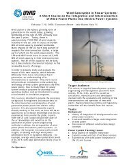
A subset of the NREL wind plant dataset was selected from the SPP footprint to meet the energy
goals for the regions included in the study. The plants were selected based on several criteria
beyond simple geography. Plants over 1000 MW were eliminated from the pool as they tend to
understate the geographic diversity obtained by combination of smaller plants. The highest
capacity factor plants were kept and an effort was made to include significant resources in all
states in the SPP footprint.
This reduced the number of plants for selection to 419 totaling 190 GW of nameplate capacity.
The locations of these plants can be seen in Figure 3-1.
Figure 3-1
Location and size of the wind plant selection pool

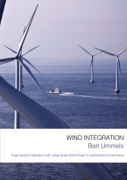
The study team determined that any scenario where wind from SPP was moved into the SERC
study region would most likely have the wind plants serving each region distributed across the
footprint. This served to maximize the aggregation benefits for each region. The effects of
aggregation are discussed in the next section.
A prior study performed for SPP selected which plants would be used to meet the 20% energy
target for SPP. These same plants were utilized for SPP in this study. To assign plants to
Entergy, Southern Company and TVA, random selections were made from the list of plants until
each region’s energy target was met. The plants were assigned to their respective regions and
that assignment was carried through into the production cost modeling. Figure 3-2 shows the
results of that process. The aggregate statistics from wind production from these plants is
presented in the Wind Characteristics section.
Figure 3-2
Assignment of wind plants to regions
Effect of Aggregation of Wind Plants
As the number of plants and particularly the geographic diversity of those plants increases, the
variability of the output of the aggregated plants decreases. As noted, the wind plants selected
to comprise the wind generation for each of the regions in the study were selected to provide
geographic diversity. This has several consequences. Given the set of wind plants and the
geographic area covered, this minimizes the variability seen for each of the regions. A different
3-3

site selection could have congregated the plants for each of regions in a smaller area, correlating
the output to a higher degree and resulting in higher variability. This has direct consequences to
the results of the study since the lower the variability, the lower the balancing requirement for
wind. This assumption of higher diversity tends to reduce the inter-BA cooperation benefits that
are calculated later.
To illustrate, Figure 3-3 shows these diversity effects for an example set of plants from the actual
data used in the study. Using the standard deviation of the 10 minute change in aggregate output
as a metric, the variability of eight concentric aggregation areas is examined. The smallest is a
single 100 WM plant moving in steps to the largest of a 12000 MW regional aggregation. Note
that variability drops from more than 4.5% for the single plant to about 1% for the largest
aggregation area.
This aggregation has a direct effect on reserve requirements and ramping duty seen by the entity
who balances the wind. If the wind is rising in one portion of the aggregation area, as the size of
the area increases, it is much more likely that it is decreasing in another portion to reduce the size
of the net change.
Normalized 10 minute Sigma
5.0%
4.5%
4.0%
3.5%
3.0%
2.5%
2.0%
1.5%
1.0%
0.5%
0.0%
Effect of Geographic Diversity and Aggregation on Variability
Normalized to Aggregate Wind
0 2000 4000 6000 8000 10000 12000 14000
Total Aggregated Nameplate (MW)
Figure 3-3
Effect of diversity and aggregation on variability
Wind Characteristics
With the wind plants selected and assigned to the four study regions, aggregate wind data can be
calculated and characteristics computed. Table 3-2 shows these characteristics tabulated with the
coincident total and non-coincident total for the entire footprint.
3-4

Table 3-2
Characteristics of aggregated wind plants
Entergy SOCO SPP TVA
3-5
Total
(Coincident)
Nameplate (MW) 7850 14999 14692 10368 47909
Total (non-
Coincident)
Maximum Output (MW) 7170 13541 13229 9366 43067 43306
Total Energy (GWh) 28537 55441 52216 37499 173693
Average Output (MW) 3231 6277 5912 4246 19666
Capacity Factor 41% 42% 40% 41% 41%
Apparent Capacity Factor* 45% 46% 45% 45% 46%
10 Minute Ramps
Max Up Ramp (MW) 665 1349 918 899 2588 3830
Average Up Ramp (MW) 68 110 110 85 303 374
Max Down Ramp (MW) 747 1010 866 820 2545 5988
Average Down Ramp (MW) 65 105 106 83 292 650
1 Hour Ramps
Max Up Ramp (MW) 1565 2781 2768 1912 7457 9025
Average Up Ramp (MW) 255 464 480 342 1438 1540
Max Down Ramp (MW) 1427 2638 2991 2151 8635 17842
Average Down Ramp (MW) 253 448 466 337 1384 2889
*Apparent Capacity Factor is the ratio of the average output to the maximum output as opposed to the nameplate
capacity.
The maximum output shown is significantly less that the nameplate for several reasons. First,
the wind rarely blows everywhere at once so not all turbines assigned to a region are at full
output at the same time. When the wind is blowing at very high speeds, high speed cut-outs of
turbines also occur. When the production data was calculated, losses, both electrical and wind
related are taken into account further reducing the maximum output from nameplate.
Comparing the energy values in Table 3-2 to the energy requirements in Table 3-1 shows slight
variations from the targets. This is due to the granularity of the plants making it impossible to
meet the target exactly. The actual total is within about 1% of the target.
Variability of wind plants is a measure of how much and how often the output of the plant
changes. While statistics give a high level picture of that variability, it is useful to look at
specific examples of how the wind output varies hour to hour. Figure 3-4 shows two separate
weeks from the wind output data at an hourly resolution. The first week shows a typical week in
the spring. The changes in output can be relatively sudden, with extreme changes typically due
to the passage of weather fronts. The second week is from summer where a diurnal pattern can
be observed. In both cases, the wind production data for the four regions in the study footprint
are highly correlated on timeframes in the tens of minutes to hour. The subject of variability and
how it relates to reserves is reviewed in detail in subsequent sections of this chapter.

Wind Production (MW)
Wind Production (MW)
14000
12000
10000
8000
Typical Spring Week
6000
4000
SPP
Entergy
2000
SoCo
0
TVA
6-Apr 7-Apr 8-Apr 9-Apr 10-Apr 11-Apr 12-Apr 13-Apr 14-Apr
10000
9000
8000
7000
6000
5000
4000
3000
2000
1000
Typical Summer Week
0
15-Aug 16-Aug 17-Aug 18-Aug 19-Aug 20-Aug 21-Aug 22-Aug
Figure 3-4
Sample weeks of wind output for the study regions
An interesting and important characteristic of wind production is the size and duration of wind
ramps that the system will experience. Based upon the one year of data analyzed for this study,
Figure 3-5 shows the maximum expected ramp magnitude and duration for each region. The
method used to create this data looks at every possible ramp within the data and tabulates the
maximum up and down ramp seen at each duration.
3-6
SPP
Entergy
SOCO
TVA

Ramp Magnitude (MW)
15000
10000
5000
0
-5000
-10000
-15000
Figure 3-5
Wind ramp envelopes seen for each region
Because the method used to select the wind plants for each region gave a very even distribution
of plants across the SPP footprint, the wind production for the four regions is highly correlated.
This can be seen clearly looking at the two of the most extreme events seen in the data as shown
in Figure 3-6 and Figure 3-7, where extreme is defined as the greatest magnitude changes and
ramp rates.
Wind Delivery (MW)
14000
12000
10000
8000
6000
4000
2000
Figure 3-6
Worst long term event
Magnitude and duration of wind ramps
0 2 4 6 8 10 12
Ramp duration (Hours)
Worst Long Term Event
SPP Entergy
SoCo TVA
3-7
Entergy
SOCO
0
0:00 2:00 4:00 6:00 8:00 10:00 12:00 14:00 16:00 18:00 20:00 22:00
Time in Hours
SPP
TVA

Wind Delivery (MW)
12000
10000
8000
6000
4000
2000
0
0:00 1:00 2:00 3:00
Time in hours
4:00 5:00 6:00
Figure 3-7
Worst short term event
In addition to the wind production data, the dataset for this study also contained a day-ahead
forecast of the wind production that exhibited the approximate error characteristics of current
state of the art forecast models. Individual wind plant forecasts have an MAE (mean absolute
error) of 17% on average for all of the sites used in the study. However, the aggregation effects
discussed earlier apply to the forecasts as well. The statistics for the forecast for each of the
regions is shown in Table 3-3. These DA forecasts of wind output are used in the day-ahead
commitment process of the SCUC/SCED simulations ensuring that the actual DA forecast errors
have to be accommodated during the real-time dispatch using resources online or expensive
quick start generation.
Table 3-3
Wind production forecast error statistics
Worst Short Term Event
ENTERGY SOCO SPP TVA Footprint
MAE %Nameplate 8.3% 7.6% 8.6% 8.0% 7.7%
MAE MW 653 1141 1268 829 3710
Max Error 37% 35% 44% 35% 37%
Reserve Requirements
The increased variability and uncertainty from wind power causes an increase in operating
reserve requirements. Those requirements have to be provided by some combination of flexible
generation and responsive load. Together, these contribute to the operating reserve that is
available to help manage the wind and load variability. This reserve is calculated dynamically,
and is a function of the observed variability of the wind power and the load. A methodology was
developed to estimate the increased requirements for reserves with wind variability in the
Eastern Wind Integration and Transmission Study (EWITS).
Short-term variability is challenging because it is difficult to fully anticipate the scheduling
changes and fluctuations that must be covered with reserves. In a system with 10-minute or
faster dispatch update cycles, a typical approach is to forecast a flat value for wind output for the
3-8
SPP Entergy
SoCo TVA

next interval based on the past 10 to 20 minutes (persistence forecast). The wind varies on that
time scale, and an understanding is needed of how it will vary during the forecast interval.
Figure 3-8 and Figure 3-9 illustrate how the forecast error is calculated for both 10-minute and 1hour
dispatch schedules for this study. The forecast error is the difference between the actual
data and the forecast value.
Figure 3-8
Forecast for 10-minute dispatch
Figure 3-9
Forecast for 1-hour dispatch made at 40 minutes prior to the beginning of the operational period
An estimate of the reserve requirements can be made using a statistical approach. Based on
detailed load, wind and forecast data, the standard deviation or other variability metric can be
used to calculate this estimate.
For this study, the reserve requirements are broken down into three classes by the types of
resources required to fulfill them (Types 2 and 3 are both types of contingency reserves):
3-9

1. Regulation is required to cover fast changes within the forecast interval. These changes
can be up or down and can happen on a minute-to-minute time scale. Regulation requires
resources on automatic generation control (AGC).
2. Spinning reserve is required to cover larger, less frequent variations that are primarily
due to longer-term forecast errors. Spinning reserve is provided by resources (generation
and responsive load) that are spinning and that can fully respond within 10 minutes.
These resources do not necessarily require AGC.
3. Non-spinning and supplemental reserves are used to cover large, slower-moving,
infrequent events such as unforecasted ramping events. Non-spinning reserve can be
made available within 10 minutes and can come from quick start resources and
responsive load. Supplemental reserves can be made available within 30 minutes.
Calculation Methods
At the root of the reserve requirement calculation method is the observation that the variability of
wind plant output is a function of its production level and that the short-term variability in wind
plant output and thus short-term forecast error is a normally distributed. Through analysis, an
equation can be written for the standard deviation (sigma) of wind variability as a function of
wind production level. That equation is derived by analyzing the wind production data over
some long period of time (a year or more), sorting the data into ranges by production level and
calculating the standard deviation for the variability in various ranges of wind output. Figure
3-10 shows an example of this function.
Sigma of Forecast Error (MW)
120
100
80
60
40
20
0
Short-term Forecast Error Sigma vs. Production Level
0 1000 2000 3000 4000 5000 6000 7000
Wind Production Level (MW)
Figure 3-10
Short term forecast error sigma as a function of wind production level
3-10

The polynomial shown in Equation 1 is the curve fit shown as the smoothed line in Figure 3-10.
Equation 1 - Sample calculation of hourly wind standard deviation
The equation is used to calculate the standard deviation (sigma) of the wind power for each hour.
A component to cover load variability is calculated as a fixed percentage of the hourly load.
That fixed percentage is as 1.5% of the hourly load in each BA and is calculated to cover 3
standard deviations of the load variability. The wind component is scaled to 3 standard
deviations and combined with the load component as the square root of the sum of the squares as
shown in Equation 2.
Equation 2 - Calculation of intra-hour regulation requirement
The 3-sigma approach estimates reserve values that will cover 99.7% of all short-term variability
for normal distributions which is generally true for the short term forecast error. This component
must be covered by regulating reserves under AGC.
An additional uncertainty reserve component to cover hour-ahead wind forecasting error was
calculated. This component is calculated in a similar manner to the short-term forecast error
described above, using an equation to describe the standard deviation of hour-ahead forecast
error. Figure 3-11 shows the development of the equation for hour-ahead forecast error standard
deviation.
Sigma of Forecast Error (MW)
450
400
350
300
250
200
150
100
50
0
Hour-ahead Forecast Error Sigma vs. Production
Level
0 1000 2000 3000 4000 5000 6000 7000
Wind Production Level (MW)
Figure 3-11
Hour-ahead forecast error sigma as a function of wind production level
3-11

The polynomial shown in Equation 3 is the curve fit shown as the smoothed line in Figure 3-11.
Equation 3 - Sample calculation of hour-head wind standard deviation
With this equation, the expected standard deviation for the forecast error is calculated based on
the previous hour’s production (persistence forecast). This component helps to insure the system
is positioned with enough maneuverability to cover the probable forecast error and divided as 1
sigma assigned to spinning reserves and 2 sigma assigned to non-spin/supplemental reserves.
Equation 4 shows the function for the spinning reserves. The equation for nonspinning/supplemental
reserves is the same except that 2 * sigma is used.
Equation 4 - Calculation of spinning reserves requirement
To calculate the total reserve requirement, each of these three components, regulation, spin and
non-spin, are added arithmetically.
Results
The method described above was applied to each of the scenarios defined for this study. The
details of those scenarios are documented in chapter 4, but Table 3-4 shows a summary of the
wind variability allocations to regions by scenario for reference.
Table 3-4
Balancing responsibility by scenario
Scenario Description
1 SPP manages intra-hour variability for all wind
2
3 & 4
Each region manages intra-hour variability for the wind assigned to their
region
All regions are combined into a single super-region and intra-hour
variability is managed jointly
3-12

Table 3-5 shows the contingency reserve values used for each of the regions as modeled for the
scenarios. For scenarios 3 and 4 where the regions in effect operate as a single balancing area,
the contingency reserve was assumed to be the highest value from each of the regions. Here, only
the single largest contingency is counted towards contingency reserve across the entire footprint;
this reduction is not due to wind but the fact that only one contingency is now examined.
Another approach would have been to count the two largest contingencies, as there would be a
higher probability of multiple simultaneous outages. This would tend to lessen the aggregation
benefit as the reduction in the aggregate reserve requirement would be less.
Table 3-5
Contingency reserves
Scenario Area Spin Non-spin
SPP 800 800
1 and 2
Entergy
Southern
1020
650
1020
600
TVA 300 1300
3 and 4 All 1020 1020
For all scenarios, a load regulation requirement of 1.5% of the hourly load was included in the
total regulation requirement (load and wind).
Figure 3-12 shows the average regulation (load and wind) for all scenarios (with the bars
representing maximum). Figure 3-13 and Figure 3-14 show the average total reserves
(regulation, spin and supplemental) without and with contingency reserves included,
respectively. The whiskers on the plots show the maximum values.
In scenario 1, SPP receives the greatest possible wind aggregation benefit since all of the wind is
aggregated into a single pool. However, SPP only benefits there are no load aggregation benefits
in this scenario since the regional loads have not been combined.
In scenario 2, there are slightly less wind aggregation benefits because the wind has been
allocated to the individual regions for balancing. Since the wind is being netted with a much
larger pool of load the net regulation for the overall footprint is decreased. The reduction in
regulation is offset by a higher spin and supplemental to make the total reserves nearly the same
for scenarios 1 and 2. Regulation is reduced in the footprint by 206 MW while spin and
supplemental are increased by 118 MW and 235 WM, respectively, leading to a 147 MW
increase in total reserves for the footprint in scenario 2.
Scenarios 3 and 4 are identical for the reserve requirements and are labeled as scenario 4 on the
graphs. These scenarios see a reduction in regulation and total requirements due to the
aggregation of all load and wind into a single balancing area. The overall footprint regulation
requirement is reduced about 190 MW over scenario 2 and 395 MW over scenario 1. The wind
related spin and supplemental components of the reserves are based on the aggregated wind
making these components the same for scenarios 1 and 4. There is a reduction of 118 MW and
235 MW for spin and supplemental from scenario 2 to 4. The reduction in total reserves is 542
MW in the same scenarios.
3-13

Regulation (MW)
Figure 3-12
Summary of regulation requirements for each scenario
Total Reserves* (MW)
4000
3500
3000
2500
2000
1500
1000
500
0
12000
10000
8000
6000
4000
2000
0
Regulation
SPP Entergy Southern TVA Footprint
Total Reserves (Regulation, spin and supplemental)
SPP Entergy Southern TVA Footprint
Figure 3-13
Total reserves (regulation, spin and supplemental but excluding contingency) for each scenario
The dramatic reduction in total reserves with contingency reserves included is because for
scenario 3 and 4, the regional contingency reserves are aggregated by using the maximum of the
regional requirements. Figure 3-14 shows the total reserves with the contingency requirements
added to the load and wind related values from Figure 3-13. There is nearly a 5000 MW
reduction in total reserves for scenario 4 over scenarios 1 and 2. All but about 550 MW of this
reduction is due to consolidation of contingency reserves.
3-14
14GW
SC1
SC2
SC4
14GW
SC1
SC2
SC4

Total Reserves (MW)
18000
16000
14000
12000
10000
8000
6000
4000
2000
0
Total Reserves including contingency
SPP Entergy Southern TVA Footprint
Figure 3-14
Total reserves requirements including regional contingency requirements
3-15
14GW
SC1
SC2
SC4

4
HIGH WIND TRANSFER SCENARIO DECRIPTIONS
This study used scenario analysis to quantify the cost of meeting the increased balancing
requirements associated with four SERC BAs (TVA, Southern Co, Entergy, and Oglethorpe
Power) obtaining large amounts of energy from wind generation that is physically located within
the SPP footprint. There are numerous ways that power system reliability could be maintained as
large amounts of wind generation are added to the power system. Wind generation will increase
variability and uncertainty making balancing generation and load more difficult. 1
A fundamental
assumption underlying the study methodology is that power system reliability will be
maintained. Reserves will be increased and operating practices adjusted to accommodate the
increased variability and uncertainty imposed by the increased wind generation. Required
changes in unit commitment and economic dispatch will tend to increase costs. These increased
costs were quantified with production cost modeling.
Four scenarios were developed to examine different methods for reliably dealing with the
increased variability and uncertainty associated with increased wind generation. These scenarios
span a range of balancing options. In all cases the new wind resources are physically located in
SPP although the entities with the obligation to increase their renewable generation portfolios are
in SERC as well as SPP. In all cases the wind plants “assigned” to each SERC load serving
entity were spread geographically throughout SPP. All of TVA’s wind plants could have been
geographically clustered together, for example. This would have reduced the diversity and
further increased the balancing costs for each of the SERC BAs. We did not elect to model this
low diversity case. The study team determined that any scenario where wind from SPP was
moved into the SERC study region would most likely have the wind plants serving each region
distributed across the footprint.
The scenarios are numbered in order of increasing cooperation and expected decreasing
balancing cost. Scenario 4 is described before scenario 3 because scenario 3 is a more
complicated version of scenario 4.
Scenario 1: SPP Provides all Within-Hour Balancing
Scenario 1 imposes the entire within-hour balancing obligation on SPP. Wind is scheduled to
each of the SERC BAs hourly but SPP deals with the within-hour forecast uncertainty and the
inherent variability of the entire wind fleet. SPP does get the natural aggregation benefit of only
having to balance the net variability and uncertainty of the wind generation assigned to all four
SERC BAs rather than having to balance each SERC BAs wind resources separately. SPP
receives the greatest possible wind aggregation benefit since all of the wind is aggregated into a
1 This study focuses on those balancing requirements and assumes that sufficient transmission will be built to both
move the wind energy to load centers and to accommodate balancing requirements. Transmission costs will likely
be significant but designing an optimal transmission network was beyond the scope of this study. If the balancing
benefits found in this study are sufficiently large then it may be worthwhile to begin investigating what
transmission investments would be required to allow the balancing savings to be realized and how those benefits
compare to the transmission costs.
4-1

single pool. However, there are no load aggregation benefits in this scenario since the regional
loads have not been combined.
The study team did not expect this scenario to be viable. The expectation was that SPP would not
have sufficient reserves and flexible resources to be able to reliably balance this much additional
wind generation. The scenario was defined simply as an extreme end of the balancing spectrum.
A proxy case for Scenario 1, with wind forecasts assumed perfect and no additional reserves
needed to cater for intra-hour variability and uncertainty in wind, is also examined, to quantify
the additional balancing costs incurred by wind.
Scenario 2: Dynamic Scheduling Wind to Each SERC BA
Scenario 2 dynamically scheduled each SERC BA’s wind generation out of SPP and to the
SERC BA. Each BA aggregates its wind with its load and uses its own internal resources to
balance the net BA variability and uncertainty. This scenario increases the size of the load that
wind is aggregated with and increases the pool of responsive generation but looses the
aggregation benefits associated with combining the variability and uncertainty of all of the wind
fleet together.
Scenario 4: Reserves Shared Throughout SPP and the SERC BAs Without Hurdle
Rates
Scenario 4 provides the largest aggregation benefit. All of the resources throughout SPP and the
SERC BAs are available for balancing and the balancing obligation is reduced through
aggregation of the footprint wide variability and uncertainty of both wind and load. The regional
contingency reserves are also aggregated by using the maximum of the regional requirements.
The day-ahead unit commitment is done based upon each BAs obligations and expectations but
the real-time balancing is optimized over the footprint.
Scenario 3: Reserves Shared Throughout SPP and the SERC BAs With Hurdle
Rates
Scenario 3 is similar to scenario 4 in its aggregation benefits and reserve requirements but there
are hurdle rates between the BAs that increase the cost of inter-BA transactions.
4-2

5
HIGH WIND TRANSFER CASE RESULTS
This chapter examines results from the High Wind Transfer scenarios described in the previous
chapters. As noted in Chapter 2, all of the high wind transfer cases utilize the Transportation
mode solution that provides an unconstrained transmission network model so that transmission
does not curtail wind significantly. Utilizing these models, first, the impact of increasing SPP
wind generation capacity from 14 GW to 48 GW is examined briefly to provide context as to the
effect of high levels of wind on the unconstrained case so that the subsequent results are better
understood. The bulk of the chapter examines in detail the differences in the four High Wind
Transfer scenarios that are the basis for understanding the potential benefits of coordinated
scheduling and balancing throughout the SPP-SERC footprint. Generation, interchanges between
regions, costs, and reserve allocation are shown to better understand the possible benefits of
cooperation.
Impacts of Increasing Wind Penetration to Meet 20% RES
This subsection examines how generation output and flows across the SPP-SERC footprint are
impacted when wind generation capacity in SPP increases from the 14 GW level to 48 GW.
Identifying these impacts is not the primary focus of the study, but understanding the change in
generation which is due to high wind being added provides a better understanding of how the
generation and flows between regions will change as the wind is being balanced differently,
which is examined in the next section. The analysis is based on comparison of the 14 GW
“unconstrained” case described in Chapter 2 and the High Wind Transfer Scenario #1 described
in Chapter 4. Table 5-1 lists the only differences in the case setups, with all other aspects of the
cases being the same.
Table 5-1
Differences in 14 GW Unconstrained and High Wind Scenario #1 Case Setups
14 GW Unconstrained High Wind Scenario #1
Installed Wind Cap 14 GW 48 GW
Scheduling of DA Wind Forecast All to SPP Shares to SPP and SERC
Intra-Hr Reserves for Wind
Carried by SPP alone for
14 GW
5-1
Carried by SPP alone for
all 48 GW
Generation and Interchange Differences
Increasing installed wind capacity by 34 GW within the footprint obviously impacts the output
levels of other types of generation within each region and the flows between regions. Table 5-2
shows the change in average generation when wind is increased from 14 GW installed capacity
to 48 GW. As expected, wind displaces combined cycle gas (CC) and coal usage. Blue indicates
a reduction in generation, green an increase, as wind is added to the system. There is a small

(390 MW) difference in total generation; this is due to the fact that, even though flows to
MISO/PJM/WAPA were fixed from one scenario to another, the method used to fix the flows
allowed slight changes in flows if it was seen as necessary by the model. For the remaining
scenarios, flows do not change to outside regions.
Table 5-2
Increase in Average Generation Scenario 1 Relative to 14 GW Case
Change in
GW
EES TVA SBA SPP SERC-W SERC-E Total
CC (1.19) (0.41) (2.18) (0.36) (0.36) (0.06) (4.56)
GT (0.03) (0.05) (0.16) 0.21 (0.20) (0.20) (0.43)
Hydro - 0.00 0.00 - - (0.00) (0.00)
Nuclear (0.00) - - (0.00) - (0.00) (0.00)
Coal (0.09) (0.99) (0.92) (2.95) (1.58) (0.94) (7.48)
GasOil (0.34) - (0.00) (0.01) - (0.00) (0.34)
Wind - - - 13.53 - - 13.53
Other (0.01) (0.03) (0.10) (0.06) (0.03) (0.10) (0.33)
Total (1.66) (1.48) (3.35) 10.36 (2.17) (1.31) 0.39
The change in interchange between regions is shown in Table 5-3. This shows the increase in
interchange from the region along the side to the region along the top. As expected, SPP
increases exports significantly, by almost 10 GW. This is for an increase in wind generation of
13.5 GW on average. Therefore, it appears that most of the wind gets moved out of SPP, but
there is also some displacement of generation in SPP. The regions labeled ‘East’ and ‘West’ in
the table refer to the SERC regions other than those explicitly shown in the study. As the model
also allowed generation to change in these regions, these changes are shown. The regions are
split into East and West as the western regions are expected to be most affected.
Table 5-3
Change in energy export/import from region to region - positive indicates increase in export
EES TVA SBA SPP WEST EAST FRCC MISO PJM Total
EES - 556 2,062 (4,877) 913 - - 159 - (1,187)
TVA (556) - (717) - 208 (413) - - 0 (1,478)
SBA (2,062) 717 - - (2,047) 41 0 - - (3,351)
SPP 4,877 - - - 3,425 - - 1,193 - 9,494
WEST (913) (208) 2,047 (3,425) - 1,580 - (1,253) 0 (2,172)
EAST - 413 (41) - (1,580)
- (99) 0 (1,306)
FRCC - - (0) - - - - - - (0)
MISO (159) - - (1,193) 1,253 99 - - - (0)
PJM - (0) - - (0) (0) - - - (0)
Figure 5-1 shows the net effect of adding wind to the entire SPP/SERC footprint. This does not
show actual imports/exports changes between each region but rather the effect that this increase
in wind has, in terms of where energy is increasing and decreasing. As shown in the previous
two tables, SPP increases generation. This flows to all regions, with Southern Balancing
Authority (SBA) decreasing generation to about one third of the SPP increase, and other regions
5-2

decreasing smaller amounts. It is interesting to note that, even though the wind is committed day
ahead in only the Entergy, SBA and TVA regions of SERC, the other SERC regions also end up
decreasing generation in the economic dispatch phase, as it is less expensive to the entire system
that they do so.
Figure 5-1
Effect of wind on system; blue indicates and increase in generation, orange a decrease in
generation
Considerations for SPP Providing All Within-Hour Balancing for Scenario #1
The model does not show that Scenario #1, where SPP provides the within hour balancing for all
48 GW of wind, results in a loss of load reliability issue, as may have been expected when a
system with a peak of 55 GW has to manage almost 48 GW of installed wind. Although initially
unexpected by the project team, after consideration of the results, the following reasons for this
result are provided:
• High reserve margin modeled. The planned generation for the Non-RES case is
maintained for the high wind generation cases such that no plant is assumed to be retired
despite the large increase in wind generation installed as we move from the 7 GW to 48
GW case. Therefore, SPP is left with large amounts of resources, both to meet energy and
reserve requirements. Even not considering wind, it still has a reserve margin of 20%
above peak demand (and as has been shown in the past, wind will have some capacity
credit).
• Availability of reserve capable generation. Although the regulation requirements
increase to 1.6 GW and spinning reserve increased to 3 GW, there is 4.5 GW of
regulation capacity and 9.5 GW of spinning capacity. Although some of these capacities
overlap, sufficient reserves are available assuming that the commitment and dispatch
select the appropriate resources for providing energy and leaving available capacity on
5-3

the reserve capable units. Later sections will show how this may be an issue for some
hours as the resources which could otherwise be used to provide regulation are being
asked to provide energy; however, this is only for a small amount of hours and could be
remedied in reality.
• Only within-hour balancing covered by SPP. The wind generation allocated to each of
the SERC BAs is committed out to Entergy, SBA and TVA day ahead. As a result,
generation is scheduled in these BAs respectively to follow the inter-hour variability of
much of the wind generation. SPP is only required to maintain reserves to cover the
within-hour variability.
Comparison of High Wind Transfer Scenarios
This section summarizes the results of the UPLAN simulations of the high wind scenarios. The
purpose of the production cost simulations is to examine the possible effects of different methods
to balance the short term variability and uncertainty of the wind located in SPP much of which is
exported to SERC. Three different balancing/cooperation methods are examined, with
sensitivities around hurdle rates, effect of forecast uncertainty and increased reserves, and gas
prices. The section is laid out as follows: firstly, the total average generation for the different
scenarios is shown to enable quick comparison between scenarios. Next, the interchanges
between regions are examined to show how the movement of energy around the system is likely
to change with different balancing strategies. Finally, production costs are compared across all
regions to quantify benefits. Having compared across all scenarios, comparisons between
individual scenarios are shown in more detail, again concentrating on changes in generation and
interchange. The reserve requirements and provision by unit type and region are then shown – as
the focus of the study is different methods to carry this reserve, these results help explain many
of the differences between scenarios. More detail is then given on start-ups and capacity factor of
units. A sensitivity on gas prices is examined last. It should be noted that all results are based on
the particular modeling assumptions utilized, including both on input data (e.g. fuel price, unit
characteristics, plant mix, wind time series) and operational assumptions (e.g. how the unit
commitment and dispatch is carried out, assumptions on hydro generation, assumptions about
interaction between the regions in the study and also interaction of the study regions and outside
areas, etc.).
Generation Summary
Table 5-4 shows the average generation per unit type for each region and the total for all regions.
The data shows that the changes in generation due to balancing approach are relatively small and
impact primarily CC, coal and GT. Note here the wind shown for the SERC regions is the wind
located in SPP and distributed out to the SERC regions.
Table 5-4
Average Generation in GW by region and type for all areas and high wind scenarios
Unit Type Scen. 1 Scen. 2 Scen. 3 Scen. 4
Scen. 1
Proxy
Entergy CC 2.1 2.2 2.2 2.3 2.0
GT 0.0 0.0 0.0 0.0 0.0
Hydro 0.2 0.2 0.2 0.2 0.2
Nuclear 4.9 4.9 4.9 4.9 4.9
5-4

Coal 3.6 3.6 3.6 3.6 3.6
GasOil 0.7 0.7 0.7 0.7 0.7
Wind 3.7 3.7 3.7 3.7 3.7
Other 0.1 0.1 0.1 0.1 0.1
Total Gen 15.3 15.4 15.4 15.5 15.2
SBA CC 5.0 5.7 4.2 3.2 4.9
GT 0.1 0.1 0.1 0.1 0.1
Hydro 0.8 0.8 0.8 0.8 0.8
Nuclear 7.4 7.4 7.4 7.4 7.4
Coal 14.7 14.5 15.0 14.4 14.8
GasOil 0.0 0.0 0.0 0.0 0.0
Wind 6.3 6.3 6.3 6.3 6.3
Other 0.7 0.7 0.8 0.7 0.7
Total Gen 34.9 35.4 34.5 32.8 35.0
TVA CC 1.5 2.1 1.1 1.4 1.5
GT 0.1 0.3 0.0 0.0 0.1
Hydro 2.0 2.0 2.0 2.0 2.0
Nuclear 8.3 8.3 8.3 8.3 8.3
Coal 10.8 10.5 11.0 10.9 10.9
GasOil - - - - -
Wind 4.2 4.2 4.2 4.2 4.2
Other 0.4 0.4 0.4 0.4 0.4
Total Gen 27.4 27.8 27.1 27.3 27.4
SPP CC 3.1 2.3 2.3 2.9 2.1
GT 0.5 0.1 0.1 0.1 0.1
Hydro 0.8 0.8 0.8 0.8 0.8
Nuclear 2.2 2.2 2.2 2.2 2.2
Coal 19.2 19.4 20.1 21.0 20.0
GasOil 0.0 0.0 0.0 0.0 0.0
Wind 5.9 5.9 5.9 5.9 5.9
Other 0.8 0.8 0.8 0.8 0.8
Total Gen 32.6 31.6 32.2 33.8 32.0
SERC East CC 2.2 2.1 2.2 2.2 2.2
GT 0.6 0.6 0.6 0.7 0.6
Hydro 1.0 1.0 1.0 1.0 1.0
Nuclear 10.4 10.4 10.4 10.4 10.4
Coal 19.7 19.7 20.0 20.0 19.9
GasOil 0.0 0.0 0.0 0.0 0.0
Wind - - - - -
Other 0.6 0.6 0.6 0.6 0.6
Total Gen 34.4 34.4 34.8 34.8 34.6
SERC
West
All
regions
CC 1.4 1.5 1.5 1.4 1.5
GT 0.3 0.2 0.3 0.3 0.3
Hydro 0.0 0.0 0.0 0.0 0.0
Nuclear - - - - -
Coal 8.4 8.3 8.8 8.7 8.6
GasOil - - - - -
Wind 0.1 0.1 0.1 0.1 0.1
Other 0.0 0.0 0.0 0.0 0.0
Total Gen 10.3 10.3 10.9 10.6 10.6
CC 15.3 15.9 13.5 13.4 14.2
GT 1.6 1.4 1.2 1.3 1.2
5-5

Hydro 4.8 4.8 4.8 4.8 4.8
Nuclear 33.1 33.1 33.1 33.1 33.1
Coal 76.4 76.0 78.5 78.6 77.8
GasOil 0.8 0.8 0.7 0.7 0.7
Wind 20.3 20.3 20.3 20.3 20.3
Other 2.6 2.6 2.7 2.6 2.7
Total Gen 154.8 154.8 154.8 154.8 154.8
To examine the individual regions in better detail, Figure 5-2 through Figure 5-6 show the
generation by unit type in each region for all scenarios. Figure 5-2 shows that the main change in
Entergy is an increase in CC output relative to scenario 1 for all but the proxy (balancing cost)
scenario. As each subsequent scenario represents a greater level of coordination in terms of
balancing, scheduling and reduced contingency requirements, the increasing utilization of
Entergy CCs as cooperation increases indicates that in the models utilized, they are less
expensive than other CCs (and GTs) and can displace these types of generation when allowed to
do so. From the results, it seems that Entergy would increase its participation in the region as
more cooperation is allowed.
Figure 5-2
Average hourly generation in Entergy
5-6

Figure 5-3
Average hourly generation in SBA
Figure 5-3 shows the SBA average generation by unit type for the different high wind scenarios.
This shows relatively significant changes for both CC and coal for different balancing and
reserve provision strategies. SBA CC usage increases from Scenario 1 to Scenario 2, as each of
the regions becomes responsible for balancing the intra hour variability and uncertainty in the
wind assigned to them from SPP. This corresponds to a small decrease in coal. For scenario 3,
when all regions share the with-in hour reserve requirements, SBA coal output increases and CC
decreases. This would be expected as the assumptions on fuel price in the model mean coal is
significantly cheaper across the footprint, and so production is maximized, while CC in SBA is
modeled as more costly and therefore decreases generation when not needed to provide reserve.
Figure 5-4: Average hourly generation in TVA
5-7

Figure 5-4 shows the average hourly generation in TVA. Again, coal and CC change most
significantly. CC usage increases in Scenario 2 with the increase in reserve requirements for
TVA. There is an associated decrease in coal usage as more CCs are online for reserve purposes.
GTs are also used to provide reserve in Scenario 2.
Figure 5-5: Average hourly generation in SPP
Figure 5-5 shows the average hourly generation for SPP. As Scenario 2 no longer requires SPP
to balance all the additional intra-hour reserve needed for wind, there is a decrease in CC and gas
turbine usage. This allows more coal to be used, as well as decreasing the net export from SPP.
Scenario 3, where all areas balance wind and other reserve requirements together, allows for an
increase in the coal, which is modeled as cheaper than other footprint coal in this model.
Scenario 4 shows a large increase in coal usage as hurdle rates are removed and the energy
modeled as cheapest here is allowed to flow throughout the region.
5-8

Figure 5-6: Average hourly generation in all regions
Figure 5-6 shows the average hourly generation for all regions, including those other SERC
regions which also change operation across scenarios, even though none of the wind is assigned
to them. As shown before, coal and CC are most affected. CC is increased in scenario 2 as
Entergy, SBA and TVA need to provide reserve to balance the wind assigned to them. For
scenarios 3 and 4 the coal which is modeled as cheaper throughout the footprint can increase to
provide generation in response to a reduction in overall reserve requirements as well as the fact
that greater cooperation throughout the footprint allows a more optimal reserve allocation.
Interchange Summary
Table 5-5 shows the interchange, or aggregate flow of energy, between regions. These flows are
determined based on the relative economics of the generation within the different regions.
Table 5-5: Imports and exports between regions for different scenarios- positive is export
Scenario Region EES TVA SBA SPP WEST
SERC
Scenario
1
Scenario
2
Scenario
3
5-9
EAST
SERC
FRCC MISO PJM Total
EES - 86 3,139 (8,125) 365 - - 78 - (4,456)
TVA (86) - 1,070 - 991 (397) - (403) 339 1,513
SBA (3,139) (1,070) - - (2,265) 68 2,000 - - (4,406)
SPP 8,125 - - - 4,051 - - 1,387 - 13,562
WEST
SERC
(365) (991) 2,265 (4,051) - 2,088 - (1,112) 86 (2,081)
EAST
SERC
- 397 (68) - (2,088) (0) - (1) 160 (1,601)
FRCC - -
(2,00
0)
- - - - - - (2,000)
MISO (78) 403 - (1,387) 1,112 1 - - - 52
PJM - (339) - - (86) (160) - - - (585)
EES - (23) 2,731 (7,025) (121) - - 84 - (4,353)
TVA 23 - 1,309 - 1,839
(1,12
3)
- (403) 339 1,984
SBA (2,731) (1,309) - - (1,959) 71 2,000 - - (3,928)
SPP 7,025 - - - 4,181 - - 1,357 - 12,563
WEST
SERC
121 (1,839) 1,959 (4,181) - (231) - 2,024 86 (2,060)
EAST
SERC
- 1,123 (71) - 231 (0) - (3,114) 160 (1,672)
FRCC - -
(2,00
0)
- - - - - - (2,000)
MISO (84) 403 - (1,357) (2,024) 3,114 - - - 52
PJM - (339) - - (86) (160) - - - (585)
EES - 95 3,416 (8,790) 916 - - 23 - (4,340)
TVA (95) - 1,022 - 1,606
(1,23
1)
- (403) 339 1,238
SBA (3,416) (1,022) - - (2,468) 51 2,000 - - (4,856)

Scenario
4
Scenario
1 proxy
SPP 8,790 - - - 3,245 - - 1,126 - 13,161
WEST
SERC
EAST
SERC
(916) (1,606) 2,468 (3,245) - 2,112 - (375) 86 (1,475)
FRCC - -
- 1,231 (51) - (2,112) 0 - (422) 160 (1,195)
(2,00
0)
5-10
- - - - - - (2,000)
MISO (23) 403 - (1,126) 375 422 - - - 52
PJM - (339) - - (86) (160) - - - (585)
EES - (496) 2,691 (7,193) 804 - - (22) - (4,216)
TVA 496 - 2,860 - (2,831) 1,025 - (403) 339 1,485
SBA (2,691) (2,860) - - (3,407) 384 2,000 - - (6,573)
SPP 7,193 - - 0 6,154 - - 1,450 - 14,796
WEST
SERC
EAST
SERC
(804) 2,831 3,407 (6,154) - 715 - (1,847) 86 (1,767)
FRCC - -
- (1,025) (384) - (715) (0) - 772 160 (1,193)
(2,00
0)
- - - - - - (2,000)
MISO 22 403 - (1,450) 1,847 (772) - - - 52
PJM - (339) - - (86) (160) - - - (585)
EES - 37 3,076 (8,171) 513 - - 49 - (4,495)
TVA (37) - 1,165 - 2,835
(2,34
1)
- (403) 339 1,557
SBA (3,076) (1,165) - - (2,202) 57 2,000 - - (4,385)
SPP 8,171 - - (0) 3,569 - - 1,295 - 13,035
WEST
SERC
EAST
SERC
(513) (2,835) 2,202 (3,569) - (296) - 3,130 86 (1,796)
FRCC - -
- 2,341 (57) - 296 - - (4,123) 160 (1,383)
(2,00
0)
- - - - - - (2,000)
MISO (49) 403 - (1,295) (3,130) 4,123 - - - 52
PJM - (339) - - (86) (160) - - - (585)
Table 5-5 shows that flows to MISO and PJM change somewhat for different cases; however the
net exchange to these is fixed in each hour; what changes is where this comes from in the study
footprint. Therefore this does not significantly affect results.
Figure 5-7 shows the net flow from each region, as given in the last column of Table 5-5. It can
be seen that the other SERC regions also change. However, they do not change as much as those
utilities with wind assigned in the study. Notable results here include the fact that Entergy does
not change significantly in the different scenarios, as also shown earlier with generation.
However, the average flows between Entergy and individual regions change significantly; for
example Entergy goes from exporting 3.1 GW on average in Scenario 1 to SBA, to 2.7 GW in
Scenario 2. It can be seen that Entergy is thus importing less from SPP and exporting less to

SBA. More details on these types of changes are given for individual scenario comparisons later.
Other aspects of interest include the fact that SBA imports increase significantly if hurdle rates
are removed. While this assumption is likely unrealistic, it does show that, for the prices and
plant mix assumed in the model, hurdle rate levels are impacting the flow of energy; removing
them entirely can be thought of as the extreme case. In reality, these may be needed to pay for
transmission and so additional wind, with its required additional transmission may actually
increase hurdle rates.
Figure 5-7: Average net flow by region
The changes in imports/exports between scenarios are obviously very dependent on relative
economics between regions. From hour to hour, the average net flow between any two BAs may
be in the opposite direction of the average values across the year. For example, there would
likely be periods when low wind power output from the wind plants in SPP, coupled with other
load and generation differences, would result in a change in the general flow of energy across the
footprint such that Entergy or SBA would be net exporters and SPP a net importer. The data
shown in Table 5-5 and Figure 5-7 only show average flows. Additionally, different assumptions
about plant mix in each region and relative fuel prices will change the flows. The specific flow
results shown here are dependent on the modeling assumptions utilized for our study. The
results do show, however, that different strategies to balance the intra-hour variability and
uncertainty inherent in wind power will cause changes in how energy is moved across the large
region.
Production Cost Summary
This section describes the differences between production costs for different cooperation
scenarios to provide an understanding of the magnitude of impact different balancing strategies
may have on costs. As with any production cost model for future year scenarios, the absolute
5-11

magnitude of the costs are dependent on the modeling assumptions. As such, the absolute cost
values presented should be taken as indicative only with the real emphasis being on the change in
costs between scenarios. Table 5-6 shows total production costs for each region; these are costs
of generation only and therefore do not reflect the fact that one region may be importing while
the other may be exporting. The generation costs include the short run fuel, O&M and start costs,
and do not include any representation of capital expenditures.
Table 5-6: Production costs ($M)
2010 $ Scenario 1 Scenario 2 Scenario 3 Scenario 4 Scenario
1 proxy
Entergy 4,147 4,214 4,162 4,246 4,093
SBA 9,959 10,301 9,563 8,755 9,904
TVA 6,674 7,135 6,431 6,590 6,679
SPP 9,265 8,290 8,350 8,926 8,329
East SERC 12,303 12,273 12,480 12,505 12,391
West SERC 4,269 4,293 4,539 4,414 4,369
Total Costs 46,618 46,506 45,524 45,435 45,765
Total Costs/MWh 34.37 34.28 33.56 33.49 33.74
The same cost results are shown graphically in Figure 5-8. As expected from the generation and
flow results, the changes are relatively small from scenario to scenario. Entergy and the other
SERC regions not assigned wind can be seen to change very little. SPP as expected decreases in
costs when no longer required to carry all the additional reserve for wind. SBA generation costs
decrease for Scenario 3 and 4 versus Scenario 2, as the region imports more due to the modeled
cheaper units in SPP and Entergy. TVA sees a large increase in generation costs in Scenario 2,
while other scenarios are similar in costs. SPP increases its costs in Scenario 4, as its coal is
increased to be moved to the SBA region, which is assumed to have more expensive modeled
units which are turned off when hurdle rates are removed.
5-12

Figure 5-8: Total production costs for different regions for different scenarios
Figure 5-8 shows that there is significant savings for SPP moving from Scenario 1 to Scenario 2,
while Entergy, Southern, and TVA see an increase in costs as they pick up the reserve
requirements for the wind allocated to them. Scenario 3 does not show a significant difference
for SPP, but does show a significant change in costs for other regions. Considering both the costs
and generation tables shows that moving from Scenario 2 to Scenario 3 where there is increased
cooperation in scheduling and balancing across the footprint, allows more usage of SPP and
West SERC coal displacing CC usage in Entergy, SBA and TVA, which are modeled as more
expensive options.
Table 5-7: Change in production costs vs. Scenario 1
2010 $ Scen #2 Scen #3 Scen #4
5-13
Scen #1
proxy
Decrease vs. Scen #1 (M$) 112 1,094 1,182 852
% decrease vs. Scenario 1 0.2% 2.3% 2.5% 1.8%
Decrease vs. Scen #1 ($/MWh) 0.1 0.8 0.9 0.6
Table 5-7 shows the change in production costs for all scenarios relative to Scenario 1. The data
show the scale of benefits that were calculated for increasing levels of coordinating reserve
requirements and scheduling/dispatching resources throughout the SPP/SERC footprint.
Scenario #2, where each BA schedules its own resources and carries reserve for its own wind, is
slightly less costly (less than half a percent) than Scenario #1 where SPP carries all the reserves
for the within-hour variability and uncertainty. There is very little difference between scenarios
1 and 2, showing that, with the plant mix as modeled here, reserve requirements are essentially

moving from being provided by SPP CCs (and some GTs) to other regions CCs and GTs.
Overall, this does not affect costs significantly, however, it does mean less burden on SPP.
The most significant benefit is realized in moving to Scenario 3, where all of the scheduling,
balancing, and reserves are shared across the footprint. Scenario #3 results in an additional
decrease of approximately 2% of total production costs beyond the gains from Scenario 2. This
corresponds to approximately 70c/MWh relative to Scenario #2 and 80c/MWh relative to
Scenario #1. While not extremely large on a percentage basis, it does represent more than 2% of
the total annual production costs at over a billion dollars in savings. The cost saving from the
extended cooperation modeled in Scenario #3 are perhaps more meaningful viewed in context of
the savings that would be seen if the hourly wind output could be perfectly forecasted day-ahead
and had no intra-hour variability as is modeled in the proxy for Scenario 1. Removing the need
for additional reserves for wind and perfectly forecasting it day ahead saves 60c/MWh, if each
region still carried their own reserve for covering load variability and contingencies. While this
is obviously a fictitious case, it provides some context to the coordinated benefits seen in
Scenario #3 which are higher than the benefits of removing wind uncertainty.
Scenario #4 shows that removing hurdle rates does decrease the costs further beyond the
reduction from cooperation in Scenario #3, but not significantly so.
The next sections will examine in more detail differences between individual scenarios, to
pinpoint better what is happening in the model for various assumptions about balancing wind and
reducing contingency reserves.
Scen. #2 vs. Scen. #1 – Benefits of Each BA Carrying Wind Balancing Reserves
The within-region generation, between region flows, and production costs shown previously
between Scenario 2 and Scenario 1 is due to the fact that Scenario 2 increases reserves for
Entergy, SBA and TVA, with a corresponding decrease in SPP reserves. The total reserve
requirement increases slightly as described in Chapter 3. Regulation requirements decrease about
100 MW on average, while spin and non-spin increase slightly more. Table 5-8 shows the
resulting difference in generation across the footprint with positive values indicating an increase
in generation in Scenario #2 relative to Scenario #1. As noted previously, the primary impact is
that SERC BA CC and GT usage increases to carry the reserve that is dropped by SPP CC and
GT decreases.
Table 5-8: Difference** in Generation for Scenario 2 vs. Scenario 1
Change in
SERC SERC
GW EES TVA SBA SPP West East Total
CC 0.10 0.57 0.66 (0.80) 0.10 (0.01) 0.61
GT 0.00 0.21 0.01 (0.37) (0.01) (0.01) (0.17)
Hydro - - - - - - -
Nuclear (0.00) - - (0.00) - 0.00 (0.00)
Coal (0.01) (0.29) (0.17) 0.22 (0.07) (0.04) (0.36)
Gasoil 0.01 - 0.00 (0.01) - (0.00) 0.00
Wind - - - - - - -
Other (0.00) (0.01) (0.02) (0.04) 0.00 (0.01) (0.08)
Total 0.10 0.47 0.48 (1.00) 0.02 (0.07) 0.00
**Positive value represents increase in generation in Scenario #2 relative to Scenario #1.
5-14

The flow chart shown in Figure 5-9 summarizes the generation impacts across the footprint when
moving from SPP carrying all intra-hour reserves for the wind to each BA managing its own
wind’s within-hour reserves. Note that the lines between regions in do not show the change in
specific flows or interchanges between regions, but rather the change in net export for a given
region and general “direction” of the change. An orange color indicates a decrease in generation
and corresponding increase in exchanges scheduled into the area. A blue color indicates an
increase in generation and corresponding increase in energy scheduled out of the region. It can
be seen, from Table 5-8 and Figure 5-9 that the change in balancing strategy to have SERC BAs
balance their on within-hour wind variability and uncertainty (Scen #1 Scen #2) moves
conventional generation from SPP into the other areas. This increases their production costs
while decreasing SPP’s (production cost here is per MWh production in the region).
Figure 5-9: Change in generation across the footprint from Scenario 2 vs. Scenario 1; lines are not
actual interchanges but indicate where change in generation goes
As noted previously, Scenario 2 shows very little overall production costs benefits. The benefits
that are identified are due to the fact that SPP no longer needs to carry all the within-hour
balancing reserves for the wind it is exporting to the SERC regions. This is a more realistic as to
how the system would operate, as SPP would likely not carry all reserves for wind it is moving
out. From the above figure, it can be seen that, compared to the additional wind Scenario 1
moves out of SPP vs. the 14 GW case, about 10% less wind is moved out when other regions
need to keep units online to carry reserve.
5-15

It should be noted that, for Scenario 1, there are about 350 hours for which the UPLAN model
finds there is not enough available regulating capacity to ensure regulation requirements are met.
The shortage does not occur because insufficient regulating capacity exists, but rather because
the UPLAN solution prioritizes some regulating units for providing energy under the tight
system conditions where SPP is carrying all within-hour reserves. While in reality, the system
would be able to operate out of this relatively easily by bringing additional “non-regulating”
units online to free up regulating capacity, the model places more of a premium on meeting
energy requirements at low cost and therefore does not meet regulation requirements for these
hours in Scenario #1 and a smaller number of hours in Scenario #2. This is summarized in Table
5-9. For Scenarios 3 and 4 this does not happen. As can be seen, this is relatively small in
comparison to system size, however it does indicate that SPP would have to operate its system
very tightly if it had to meet regulation requirements to balance wind by itself. For some hours of
the year, the operators may find themselves needing to move units out of merit to provide
regulation.
Table 5-9: Regulation requirement violations for SPP
# Violations Avg (MW) MWh Max (MW)
Scenario 1 352 285 100548 984
Scenario 2 41 193 7942 541
Increase in SC 1 311 92 92606 443
Scen. #3 vs. Scen. #2 – Benefits of Sharing Scheduling and Reserve
Requirements
Relative to Scenario #2, Scenario #3 is modeled such that SPP, TVA, SBA, and Entergy share
resources for scheduling day-ahead and share contingency and with-in-hour reserve requirements
for the wind. As noted in chapter 3, this allows for a significant reduction in total reserve carried
due to load and wind diversity and reduced contingency requirements. Regulation decreases 200
MW and spin reduces 1900 MW due to the contingency reserve reduction. This reduction in
reserve and sharing of resources in the day-ahead commitment leads to the larger differences in
production cost results described previously.
Table 5-10: Difference** in Generation for Scenario 3 vs. Scenario 2
Change in
SERC SERC
GW EES TVA SBA SPP West East Total
CC 0.03 (1.00) (1.41) (0.03) 0.00 0.05 (2.37)
GT 0.00 (0.26) (0.03) (0.02) 0.09 0.07 (0.15)
Hydro - - - - - - -
Nuclear 0.00 - - 0.00 - (0.00) 0.00
Coal 0.03 0.50 0.47 0.62 0.50 0.32 2.45
Gasoil (0.06) - (0.00) (0.00) - 0.00 (0.06)
Wind - - - - - - -
Other 0.01 0.01 0.05 0.02 (0.01) 0.04 0.12
Total 0.01 (0.75) (0.93) 0.60 0.58 0.48 (0.00)
**Positive value represents increase in generation in Scenario #3 relative to Scenario #2.
5-16

Table 5-10 shows the difference in generation between scenarios #3 and #2. As shown earlier,
coal output from across the footprint increases significantly displacing primarily TVA and SBA
CC output. This occurs because the lower reserve requirement across the footprint results in
less need for CCs to be online and spinning and because the other SERC regions not assigned
wind (SERC West and SERC East) can now also provide reserve to balance the intra hour
variability of the wind from their cheapest generation.
Entergy’s generation contribution does not change significantly, but TVA and SBA decrease
generation corresponding to their CC decrease being greater than coal increase. SPP increases
generation due to its coal, while coal increases also account for an increase in other Western and
Eastern SERC regions. The net effect of this is a decrease in production costs of approximately
$0.7/MWh.
Figure 5-10 shows the net effect of the changes in Scenario 2 vs. Scenario 1. Entergy stays much
the same, while SPP and the SERC East and SERC West regions with no wind assigned increase
and TVA and SBA decrease generation. This results in the total cost reduction, as the cheaper
coal generation from across the footprint can be used instead of CCs in TVA and SBA.
Figure 5-10: Net effect of Scenario 3 vs. Scenario 2 - blue indicates increase in generation
Figures Figure 5-11 and Figure 5-12 show the aggregate footprint wide generation stack dispatch
for a selected week in April for Scenarios 2 and 3. This week was picked as it had high wind
variability and relatively low load, and therefore should show times when the benefits of closer
coordination can be seen.
5-17

Figure 5-11: Weekly dispatch of entire system by unit type for one week in April, Scenario 2
Figure 5-12: Weekly dispatch on entire system by unit type for one week in April, Scenario 3
This shows the small changes in dispatch which result in the difference in capacity factor and
production cost changes. Day 3 gives the clearest example where coal usage increases and the
nighttime period of April 16/17 shows no usage of CC in Scenario 3. It can be seen that CCs are
5-18

more likely to be turned off during the night in high wind days when balancing requirements are
shared.
Scenario #4 – Effect of Removing Hurdle Rates
The only difference between Scenarios #3 and #4 is that hurdle rates are removed from Scenario
#4. It was shown previously, that production costs are only slightly reduced with Scenario 4,
while generation was shown to change mainly in SPP and SBA. Table 5-11 shows the change in
generation for Scenario #4 relative to #3. Hurdle rates around SBA are highest, and therefore
SBA would be expected to show the greatest change. SPP increases CC and coal usage as these
are modeled as cheaper (cheaper fuel price, better heat rates assumptions). SBA has
correspondingly more expensive CCs and coal units. This has the effect of increasing total
interchange into SBA and out of SPP. While removing hurdle rates completely may not be
reasonable or likely (in fact they may increase as more transmission is built for wind), it does
show the bookend of what reduced rates may do in terms of impact of balancing high amounts of
wind.
Table 5-11: Difference** in average generation for Scenario 4 vs. Scenario 3
Change in
SERC SERC
GW EES TVA SBA SPP West East Total
CC 0.12 0.34 (1.05) 0.66 (0.15) (0.01) (0.09)
GT 0.00 0.01 (0.02) 0.00 0.01 0.03 0.02
Hydro - - - - - - -
Nuclear 0.00 - - 0.00 - 0.00 0.00
Coal (0.01) (0.09) (0.57) 0.92 (0.15) 0.01 0.11
Gasoil 0.01 - (0.00) (0.00) - 0.00 0.01
Wind - - - - - - -
Other (0.00) (0.01) (0.08) 0.02 (0.00) (0.03) (0.10)
Total 0.12 0.25 (1.72) 1.60 (0.29) 0.00 (0.04)
**Positive value represents increase in generation in Scenario #3 relative to Scenario #2.
Scenario #1 Proxy – Effect of Forecast Uncertainty and Increased Reserve
Requirements Associated with Wind
The scenario 1 proxy uses only the reserve requirements from the 7 GW wind case examined
earlier. Additionally, wind is assumed to be perfectly forecast. This case is analyzed to evaluate
the balancing costs that wind imposes on the system. While this does not give so-called
‘integration costs’ of wind, it does show the effect of intra-hour variability and uncertainty. This
can be used to place other costs in context. As shown earlier, the cost reduction from higher
cooperation across the footprint is larger than that which could be achieved with smaller
balancing areas if wind could be perfectly forecast and had no intra-hour variability.
The change in the average generation between the Scenario #1 and the Proxy case is shown in
Table 5-12. As expected, the largest change is in SPP, which carries all of the intra-hour
reserves for the wind in Scenario #1. Due to reduced reserve requirements, SPP CC generation
decreases and coal is increases slightly. Coal also increases elsewhere in the region reducing SPP
exports. Looking at the costs savings shown and placing them in context of savings per MWh of
wind it can be seen that the balancing costs of the wind come to approximately $5/MWh, which
5-19

is consistent with balancing costs seen in other wind integration studies, if somewhat on the low
side.
Table 5-12: Difference** in average generation for Scenario 1 vs. Scenario 1 Proxy
Change in
GW EES TVA SoCo SPP SERC W SERC E Total
CC (0.03) (0.04) (0.09) (0.93) 0.02 0.03 (1.05)
GT (0.00) 0.01 (0.02) (0.38) 0.02 0.03 (0.34)
Hydro - (0.00) 0.00 - - 0.00 (0.00)
Nuclear 0.00 - - 0.00 - 0.00 0.00
Steam
Coal
0.02 0.08 0.12 0.82 0.24 0.15 1.42
GasOil (0.03) - (0.00) (0.01) - 0.00 (0.04)
Wind - - - - - - -
Other 0.00 0.00 0.01 (0.02) 0.00 0.02 0.01
Total (0.04) 0.04 0.02 (0.53) 0.29 0.22 (0.00)
**Positive value represents increase in generation in Scenario #1 Proxy relative to Scenario #1.
Reserve Requirements and Provision
One of the significant differences in each of the High Wind Transfer scenarios is how reserves
are carried across the footprint. The changes in reserve requirements for each scenario are
presented in Chapter 3. This section examines how those reserves are provided in each of the
scenarios. Regulation up requirements and spinning reserve requirements were seen to be the
significant, and are examined here, together with total reserve requirements.
Regulation Up
The analysis of reserve requirements presented in Chapter 3 show that moving to larger areas
decreased regulation requirements, from an average of 2.2 GW in Scenario 1 to 2.1 GW in
Scenario 2 to 1.9 GW in Scenarios 3 and 4. Figure 5-13 shows the average allocation of
regulating up reserve by unit type for each of the scenarios. The first conclusion from this is the
importance of CC units to providing the regulating reserve needed, especially considering the
earlier point that some of these CCs may not be built if 48 GW of wind were to be installed.
Hydro units are also shown to be important, however, these are probably going to remain in
operation. Coal units provide less regulation in Scenario 3 as they provide more energy with the
reduced reserve requirements resulting in fewer online CCs. It can be seen that GTs are needed
in Scenario 2 to provide regulation offsetting some of the benefits of moving Scenario 1
regulation from SPP to other regions.
5-20

Figure 5-13: Average Regulation up provision by unit type
Figure 5-14: Average regulation up provision by region
Figure 5-14 shows the regulation provision by region. While total Entergy generation was shown
to remain approximately the same throughout the scenarios, it can be seen that it provides
significantly more regulation from its CCs in 3 and 4 as they tend to be less expensive based on
the inputs to this model. This means that the SBA and TVA units which provide reserve in
Scenario 2, modeled as more expensive than the Entergy units, are turned down. SPP can be seen
to carry far less regulation in Scenarios 2 and 3 versus Scenario 1, with some increase for
Scenario 4.
5-21

Spinning Reserve
Spinning reserve requirements are also reduced in Scenario 2 vs. Scenario 1, but there is a very
significant reduction in Scenario 3 as there is only need to now cover the single largest
contingency across the entire footprint. This assumption is obviously dependent on the ability to
deliver the reserves across the large area. This is also independent of the wind energy in the
footprint.
Figure 5-15 shows the spinning reserve provision by generating type for each scenario. Again,
CCs are shown to be important, even more so than for regulation. For Scenarios 3, 4 and the
proxy they serve the majority of spinning reserve requirements. In scenario 1, it can be seen that
SPP needs to use GTs quite often to provide this reserve, which would contribute to increase in
costs (offset somewhat in Scenario 2 by GTs providing regulation). Coal only provides a
significant amount of spinning reserve in Scenario 2. This figure shows clearly why moving to
coordinated balancing and reserve sharing can provide benefit. Far less reserve needs to be
allocated to coal, GTs or other units, and there is a reduction in total requirements; the CCs,
which seem to be most efficient in doing so, can carry most of the spinning reserve.
Figure 5-15: Average Spinning Reserve by unit type
Figure 5-16 shows the spinning reserve requirements by region. As expected all regions carry
less for the lower requirements in Scenarios 3 and 4. As shown earlier, CCs are modeled as
more expensive in SBA and TVA, and so their reduction is greater than for Entergy or SPP. The
fact that Entergy’s spinning reserve provision does not change between Scenarios #1 and #2
shows that this region can provide this reserve more effectively as it is modeled in this study.
5-22

Figure 5-16: Average Spinning reserve provision by region
Spinning and regulating reserve are therefore shown to cause significant changes in the
commitment and dispatch of generation throughout the study footprint. Regulation down and
non-spinning reserve, which are generally easier and cheaper to obtain, do not seem to
significantly affect results, and are therefore not examined in detail here. One point of interest is
that those regions that didn’t provide significant spin or regulation up (i.e. SBA and TVA),
provide a large share of non-spin, as offline GTs are used to provide this reserve.
Capacity Factors
While the generation levels shown before give a good indication of usage of plant, it is
instructive to look at capacity factors. These will provide insights as to the likelihood that units
may still be built if there was a large wind build-out in SPP. It also shows how much their
generation changes will impact on plant operating strategy.
Entergy capacity factor by unit type are given in Figure 5-17. For comparison, the 14 GW case is
included. This shows that there is a capacity factor reduction, of about 10% for CCs and 7% for
coal when wind is added. This may affect plant economics, but it is not clear how significantly.
Small changes throughout the scenarios can also be seen but capacity factors do not change
significantly in the high wind cases; this is consistent with earlier results for generation in
Entergy. A breakdown of the capacity factors for individual units is provided in Appendix A.
5-23

Figure 5-17: Entergy capacity factors by unit type
Figure 5-18 shows the capacity factors by unit type for SBA. As expected from results shown
previously, the change in capacity factors is more significant for SBA than Entergy. CC in
particular goes from a capacity factor of approximately 28% in the 14 GW wind case, to 22% in
Scenario 2, to 12% in Scenario 4. It can be seen therefore that different balancing strategies
would significantly affect the usage of these units, possibly changing the business case for them
being built. This is examined in more detail in Appendix A where a breakdown of the capacity
factors for individual units is provided.
5-24

Figure 5-18: SBA Capacity Factors by Unit Type
Figure 5-19 shows TVA capacity factors by unit type. These are as expected from earlier results;
showing CC units with the greatest change. Coal can be seen to decrease significantly when wind
is added, and the lowest coal usage is when TVA needs to balance the wind assigned to it in SPP
in Scenario #2. Moving to Scenario 3 allows greater utilization of the coal, which is cheaper in
the model than gas units. CC is actually used more in Scenario 2 than in the lower wind case, as
it is needed to provide reserve. Only in Scenario 3 is the capacity factor of CC units reduced by
more than 10% compared to the lower wind case. Gas turbines can also be seen to be needed
more in Scenario 2 to provide increased reserve needs. A breakdown of the capacity factors for
individual units is provided in Appendix A.
5-25

Figure 5-19
TVA Capacity Factors for Unit Type
Figure 5-20 shows the capacity factors by unit type for the year in SPP. This again reflects
earlier results. It can be seen that adding wind barely changes CC capacity factor in Scenario 1,
but reduces it by 10% in Scenario 2, where SPP no longer has to provide all of the within-hour
reserves for the 48 GW of wind. GTs can be seen to only be significant in Scenario 1 and the
lower wind cases; this indicates that at higher wind cases, they may not be built and thus not
available for reserves if needed (although earlier results indicated this may not be the case). Coal
capacity factors in SPP increases with more shared balancing requirements, from scenario 1
through scenario 4. A breakdown of the capacity factors for individual units is provided in
Appendix A.
5-26

Figure 5-20: Capacity Factors for SPP by unit type
There is little significant change in capacity factors across scenarios for the other SERC regions
across the scenarios. The eastern SERC regions (mainly VACAR) do not change noticeably,
while CCs and to a lesser extent coal change in the western regions, as shown earlier. Another
note of significance for those regions is the fact they both have significant GT capacity factors,
indicating that they use these units more than the main study regions.
Figure 5-21shows capacity factors across the entire footprint. Again, this is similar to generation
described earlier. It can be seen that much of the differences again lies in CC usage. There is a
significant decrease in CC usage in Scenarios 3 and 4 in particular, indicating that they may not
all be present in a future plant mix with this much wind. This would be crucial as these units are
shown to provide much of the reserve requirements. Alternatively, if it is shown that they are
needed to provide reserve, then they may be built, or not retired. This would impact capital cost
recovery, not studied here. Looking at the average CC capacity factor, 20% still seems relatively
high, though lower than it would be with low wind.
5-27

Figure 5-21
Capacity Factor by Unit Type across Entire Study Footprint
5-28

Unit Startups
Changing the balancing strategy can change the number of starts for units. The cost of cycling
and ramping on conventional generation in terms of effect on forced outage rate, maintenance
costs and heat rate degradation is not studied here (and is in fact not well understood in general at
present). As such, the effect of wind on cycling can only be seen from the UPLAN production
cost model results in how it changes the number of start/stop operations of units. More cycling
operation would likely result in more breakdowns, maintenance scheduling and possibly early
retirement, therefore strategies that reduce this will be beneficial, in particular for coal or older
CC units.
Figure 5-22 shows the average number of starts per year by unit type for each region. Note that
these starts are not necessarily attributable to wind variability as normal load cycling and forced
or unforced outages also drive some portion of the starts. Increased levels of wind, however,
will increase the cycling of the units. Given that the data in Figure 5-22 compares scenarios all
with 48 GW of wind, the differences between scenarios indicates how balancing cooperation
strategies impact cycling. Only CC and coal are shown as these are the units not specifically
designed to start and ramp as frequently as GTs would be. In addition, coal in Entergy is not
shown as starts do not change. As expected, coal units, which have larger start costs and times
and longer minimum up times, do not cycle on and off significantly.
Figure 5-22
Average number of starts by unit type
Table 5-13 shows the average number of starts per unit of each type per year for Scenario #1 and
the change in the number of starts for each of the other scenarios relative to Scenario 1 with a
positive value indicating an increase in starts versus scenario 1. In addition to the high wind
transfer case scenarios, the low wind case of 14 GW with unconstrained transmission is shown
for comparison of how the additional 34 GW of wind impacts unit starts. The additional 34 GW
of wind generally results in more starts in the SERC regions as more cheap and variable energy
is available, but the numbers are not as dramatic as might be expected. CC units in Entergy and
TVA cycle off on average 25 and 16 times more per unit per year in the high wind case,
5-29

espectively. Conversely, however, the number of starts on the SPP and SBA CC units decreases
by 22 and 3, respectively. The only place where there is a significant decrease in average
number of starts when wind is added is for CC units in SPP, likely as units are left online to
provide reserve. The average number of starts for each coal unit increase slightly with the
additional wind for SBA (3), TVA (3), and SPP (1). Although the numbers are small (1-3
additional starts per year per unit), they could be significant as many of these units are not likely
designed to cycle.
Table 5-13: Change in starts vs. Scenario 1
Region
Type
Scenario 1
starts
14 GW Scenario 2 Scenario 3 Scenario 4
Scenario 1
Proxy
EES CC 117 -25 -12 -2 9 -1
SOCO CC 204 3 -7 -9 -45 -6
Steam Coal 15 -3 0 2 12 1
TVA CC 240 -16 -37 -53 -11 -9
Steam Coal 7 -3 -1 1 1 0
SPP CC 84 22 103 99 88 109
Steam Coal 8 -1 0 -1 -1 -1
Comparing Scenario 2 to scenario 1, it can be seen that there is a reduction in starts for CCs in
each of the three SERC BAs when they are required to carry reserve to cover the intra-hour
variability of their wind allotment. As a result, the CCs are required to remain on line more often
to ensure sufficient reserve exists. Conversely, the CCs in SPP cycle more frequently as they no
longer have to maintain all reserves for the wind and the CCs correspondingly can be turned off
more frequently in SPP. This increase is not as significant in Scenarios 3 and 4 as the SPP CC
units are utilized more in these shared balancing scenarios due to the relative economics of these
units as modeled. On the other hand, TVA shows a larger decrease in CC starts in Scenario 3 and
SBA in Scenario 4, as these units are being turned off for longer periods of time when the less
expensive CCs in SPP and Entergy can be used to support the “shared” reserve requirement.
(Although noted previously, it should be noted again that the relative economics of the units in
different regions result from the input data utilized in the UPLAN model and may likely differ in
actual implementation in the future.) In Entergy, Scenario 4 shows an increase in CC starts
compared to other scenarios; this is also true for coal in SBA; no hurdle rates means the coal is
started more often to provide energy.
More detailed analysis of start-ups for individual CC units is presented in Appendix B.
5-30

Gas Price Sensitivity Case Results
Between the time of the start of this study and the end, projected gas prices for the 2022 study
year decreased significantly. The results of the study presented thus far are based on assumed
natural gas prices in the range of $8-$9/MMBtu, depending on region and month. Gas prices
projections near the end of the study are significantly lower, by at least $3. Therefore, the
UPLAN model was rerun for Scenarios #2 and #3 with natural gas prices reduced by $4/MMBtu
across the board to ascertain the sensitivity of the results to the gas price assumption. The effect
of the significantly reduced gas prices on the changes in production cost and generation results
between Scenarios #2 and #3 are analyzed. The main question was how differently the benefits
of increased cooperation and reserve sharing would appear with lower gas prices, i.e. how does
the total difference in scenario #2 and #3 production costs change, and how does this impact
generation.
Table 5-14 shows the change in average generation per unit type per region for Scenario 2 with
the lower gas prices. As should be expected, CC and GT generation increases displacing coal.
This resulted in an increase in generation in Entergy and SBA compared to all other areas. It
should be noted that the changes seen here are significantly greater than, for example, the
differences between Scenarios 2 and 3 shown in Table 5-10. This shows that gas prices can have
far more effect than balancing of wind generation in the generation of future power systems with
high amounts of wind.
Table 5-14
Change** in average generation for scenario 2 with lower gas price
**Positive value represents increase in generation in lower gas price sensitivity case.
The same difference in generation is shown Table 5-15 for Scenario 3 with lower gas prices.
Here it can be seen that much the same effect happens. However, gas is increased even further,
and more coal is displaced. The prior results (higher gas prices) showed that the benefit of
moving to Scenario #3 versus Scenario #2 was the ability to reduce gas generation and replace it
with coal when all resources are shared throughout the footprint. Decreasing gas prices has the
effect of reducing the benefit that can be drawn from sharing reserve. While the more efficient
reserve sources can still be shared better, there is less difference between those and other
resources, and therefore less benefit in Scenario #3 versus #2 with lower gas.
5-31

Table 5-15
Change in generation for Scenario 3 with low gas prices
The change in generation between Scenarios #3 and #2 with low gas prices is given in Table
5-16. There is now very little difference in CC usage; most of the benefits that come from
moving to larger reserve sharing areas now comes from the fact that this allows a reduction in
less efficient GTs and increase in coal. This results in small increases in generation in SPP and
the SERC non-wind regions, with a decrease in TVA and SBA where GTs had been providing
significant amounts of energy. Comparing this with Table 5-10, it can be seen that there is now
far less difference between scenarios; the benefits of cooperating across the footprint is reduced
as costs are more equal throughout the region with coal and gas being somewhat similar. There is
still a small move to more efficient (in the model) CC in SPP compared to CC elsewhere, but
total CC usage is not decreased as gas prices are so low that this is not as desirable as it was with
higher gas prices.
Table 5-16
Change in generation Scenario 3 vs. 2 low gas price
The net effect of reduced gas prices on cost is to reduce the cost difference from approx.
$0.7/MWh to approx. $0.25/MWh, a factor of three. The benefits now are not in being able to
switch from CC usage to coal when sharing reserve requirements, but the less attractive (as less
MWh) benefits of switching from GTs to coal and being able to use the more efficient coal and
CC units. It is unclear how increasing relative costs of coal (by having carbon price for example)
may affect these results. Coal may be reduced further, and shared reserve requirements may
allow greater usage of CC, but that has not been modeled.
5-32

6
CONCLUSIONS AND RECOMMENDED NEXT STEPS
The objective of this study is to evaluate the balancing/scheduling impact of high levels of wind
generation in SPP for consumption and export to SERC and to evaluate the benefits of increased
coordination in scheduling, balancing and reserve provision across the SPP/SERC region. To this
end, a detailed UC/ED model of the SPP/SERC region was developed and utilized to run
production cost simulations for different high wind transfer scenarios. As in any study like this,
modeling and data input assumptions have a significant impact on results. These assumptions
have been noted in this report with the presentation of the simulation results, but the following
most crucial assumptions provide context for the subsequent conclusions:
• Unconstrained transmission. Thermal constraints are removed and losses ignored for the
SPP/SERC network in the SCUC/SCED model for which results are presented. Analysis
to quantify the effect of unconstraining the transmission with low wind levels shows that
the assumption results in greater utilization of those resources modeled as cheaper across
the study footprint and subsequent larger economic energy flows between regions. It’s
noted, however, that any high wind build-out would necessarily be accompanied by a
significant transmission build-out that would in fact enable additional flows within and
between regions, just not to the extent modeled in this work.
• Gas and emission prices. The fuel price was shown to be important with the gas price
sensitivity. While there is always likely to be a benefit from sharing reserve requirements
and thus reducing them, fuel prices may change how significant the benefit is. This is
seen in the fact that with reduced gas prices, CC production barely changes in total, but
does shift from one region to another. Carbon prices would also impact results. Higher
carbon prices would make coal less attractive and therefore the benefits of being able to
use coal more with shared reserve requirements would be reduced.
• Reserve margin and conventional generation plant mix. The additional 40 GW of wind
was added to the High Wind Transfer cases without removing any of the conventional
generation in the 2022 Non-RES case resulting in a reserve margin in the model which
would likely be higher than that which would be seen in reality. In reality, the additional
wind would likely displace some conventional generation. Assuming for example a
capacity credit of 10% for the 40GW of wind added to the 7 GW case, then 4 GW of
conventional plant would not be required to maintain capacity adequacy at the same
level. This could lead to a reduction in the CC units which are shown to be the main
units used to provide the increased reserve and ramping needed for high penetrations of
wind. In addition, the plant mix for the conventional generation assumed in the model is
an important assumption. Although the model is based on the best information available
6-1

from the participating utilities at the time of the study, in reality, the plant mix may be
different due to impending EPA regulations.
Despite these assumptions, the results of the study provide insights as to the balancing impacts
associated with the high wind build-out in SPP and as to the benefits of increasing levels of
coordination across SPP and SERC BAs in responding to those balancing impacts. Given the
assumptions and the nature of future scenario production cost modeling, the insights tend to be
based more on the order of magnitude and trends between results than the absolute value of the
results presented.
System and Cost Impacts of High Wind
Although the focus of the study was not to conduct an evaluation of all system impacts of 48 GW
of wind on the SPP/SERC region, the analysis and modeling does provide some insight as to
certain aspects of the impact of increasing wind penetration on the unconstrained system when
comparing the results between the 14 GW and 48 GW installed wind cases.
Cost Impacts
The increase of 34 GW of wind in SPP (from 14 GW to 48 GW) results in a total production cost
reduction of approximately $5.4 billion or $4/MWh of demand. This cost reduction represents
the reduction in fuel costs from the wind generation and does not consider the offsetting cost to
purchase the wind energy or the capital/O&M costs to build the wind plants.
Comparison of the Scenario #1 and Scenario #1 proxy cases show that the costs of the intra-hour
variability and uncertainty and the day ahead uncertainty for the total 48 GW of wind in the High
Wind Transfer cases are approximately $0.6/MWh of load, or $5/MWh of wind, for Scenario 1.
This value represents most of the balancing cost that is reported in many studies as an
“integration cost.” As such, the $5/MWh of wind value is on the low end of results reported in
similar studies. This may be due to the value not including a cost associated with the inter-hour
variability (movement of conventional units to follow the perfectly known variation of wind
across the hours) and the unconstrained transmission. It should also be noted that this value does
not include any capital costs for the wind generation or transmission to deliver the wind or costs
associated with increased cycling of conventional plants due to increased ramping and start/stop
operations. The analysis does show, however, that the number of conventional generator starts
does generally increase as the wind increases, but not as significantly as might be expected for
48 GW of wind.
Generation and Reliability Impacts
The addition of 34 GW of wind in SPP (14 GW to 48 GW) for the High Wind Transfer Cases
results in wind primarily displacing combined cycle gas (CC) and coal usage. Aggregate
capacity factors for coal and CCs across the SPP/SERC footprint drop approximately 7-8% when
wind was added. This relates to the addition of the wind without retiring any conventional
generation assumption described above and may mean some units would not be present (either
retired or not built) in a high wind system. Based on the assumptions in the model on the relative
6-2

generation characteristics across regions, the average generation in TVA and SBA are reduced
the most. Additionally, it is shown that some of the wind which is committed in SPP to other
regions ends up staying in SPP resulting in coal being significantly reduced in SPP.
CCs are seen to be used most to integrate the wind, with coal and CT units also changing
operation. While all types of generation decrease output, it is clear that CC units are most used
to provide the additional reserve requirements for wind.
The most severe integration case (48 GW Scenario #1 case) where all of the intra-hour wind
variability is balanced by SPP does not result in significant reliability problems. This is due to
the fact that adding the wind capacity without removing other conventional capacity results in
high reserve margins such that there is sufficient capacity to manage the wind, assuming some of
it is committed out of SPP based on day-ahead forecasts.
Benefits of Increased Cooperation in Scheduling, Balancing, and Reserve Sharing
The analysis of the High Wind Transfer scenarios shows that increasing levels of cooperation
among SPP, Entergy, SBA, and TVA does result in changes to the operation of the system that
produce aggregate system benefits. These result from changes to the amount of reserve required
for the different scenarios. Scenarios 3 and 4 show a reduced reserve requirement due to
cooperation between regions. This is the most significant result in the study; there is a 5000 MW
decrease in total reserves needed when there is full cooperation in Scenarios 3 and 4 versus
Scenario 1. In particular, regulation needs are reduced by approximately 400 MW.
Cost Impacts
There is a clear, though possibly small, societal cost benefit to sharing the reserve requirements
throughout the region. The difference between Scenario 1 where SPP balances all wind and and
Scenario 2 where each BA balances its own wind is small – only $0.1/MWh. This is due to the
fact that the main difference in these two scenarios is to shift from using CCs and GTs to provide
reserve for wind in SPP to the same units providing it elsewhere. Comparing costs for Scenarios
2 where each BA balances their own assigned wind and Scenario 3 where balancing
requirements are shared across all BAs shows that costs decrease as result of the reduction in
aggregate reserve requirement (including contingency reserve) and a more optimal usage of the
system generation to meet energy and reserves as scheduling is shared. The cost reduction is
approximately $0.7/MWh of demand for the assumed gas prices. Reducing gas prices by
approximately 50% reduces this benefit by a factor of 3. This implies that the benefits derived
from regional coordination or cooperation are reduced as the diversity in plant mix and fuel costs
(coal vs. gas) across regions is reduced.
Removing hurdle rates reduces costs further, although the reduction in production costs is
relatively small – approx. $0.1/MWh. While it may be unrealistic that hurdle rates might be
completely removed, the analysis provides a boundary case as to the high end benefit of
6-3

cooperation. The small incremental benefit seen when hurdle rates are removed indicates that
smaller changes in hurdle rates will likely not significantly impact the results found in the study.
As for the magnitude of the benefits of increased cooperation, while all the cost differences seen
are small, they should be put in context of a total production cost reduction of approximately
$4/MWh of demand when 34 GW of wind is added. It should be noted that the cost benefit of
moving to larger scheduling/reserve areas (scenario 3 vs. Scenarios 1 and 2) are actually greater
(by approx. 25%) than if the wind could be perfectly forecast and intra hour variability flattened
out but each area still carried their own reserve (Scenario #1 and proxy).
Generation and Reliability Impacts
While the production cost impacts examine many of the benefits of increased cooperation in
scheduling, balancing and reserve-sharing, other operational insights and benefits are noted as
follows:
• There is very little difference overall in the amount and type of generation used,
particularly when moving form Scenario 1 to 2; however the location of the generation is
often changed. When regions balance their own assigned wind, they increase CC usage,
and sometimes decrease coal usage. Scenario 2 moves generation from SPP to SERC
regions, while changing very little in terms of the entire footprint.
• Moving from Scenario 2 to 3 allows more usage of the less costly units on the system. In
the model here, based on assumptions on fuel price and plant mix, this means that SPP
coal and CCs can be used more, replacing more expensive CCs from SERC in the
generation mix.
• Starts increase with amount of wind added, but then decrease for most generation (with
the exception of SPP CC) as cooperation is done on a wider basis.
• CCs can be seen to be crucial to the plant mix as they carry much of the ramping and
reserve requirements. This is true regardless of scenario or gas price.
Recommended Follow-On Work
This study has produced a SCUC/SCED model of the SPP/SERC footprint with significant
engagement and review from SPP and SERC BAs staffs. The model simulation results have
provided insights as to some of the impacts of integrating 48 GW of wind generation into the
SPP/SERC footprint and as to the benefits of increased levels of cooperation among the SPP and
SERC BAs in integrating that wind generation. While the study results provide a good basis for
understanding these issues, the underlying model contains many assumptions and the number of
sensitivities that could be performed was limited. The investigators believe that additional
insights and value could be obtained by building on the existing effort in the following ways:
• Inclusion of a conceptual transmission plan for delivering the 48 GW of wind generation.
As noted, the assumption of the unconstrained transmission is significant in that it
6-4

overstates the ability of the system to deliver energy and reserves between regions.
Including a conceptual transmission plan with all constraints and losses considered would
provide a better analysis of the magnitude of the impacts integrating the wind and the
benefits of cooperation among BAs to do so.
• Conduct additional sensitivities around fuel and emission prices. All of the results
presented are based on a single set of gas prices and no carbon price. The one sensitivity
with a sizeable reduction in gas price conducted for Scenarios #2 and #3 to bound how
the fuel assumption impacted results showed a sizeable impact. Additional sensitivity
cases should be run for varying combinations of gas and carbon prices.
• Conduct additional sensitivities around reserve margin and generation mix. The higher
than typical reserve margins in the footprint that resulted from adding the wind
generation without altering the conventional generation plan yields more flexibility in the
fleet to accommodate variability and uncertainty. Additionally, the impact of EPA
regulations on expected generation fleet in the 2022 time frame may also impact the
flexibility of the conventional generation that does exist. Further, the relative generator
characteristics across regions for the same types of units impact the flows and where
generation is produced. The SCUC/SCED model should be exercised for different
generation mix scenarios to determine the sensitivity of the results to these factors.
6-5

A
INDIVIDUAL GENERATING UNIT CAPACITY FACTORS
Entergy Individual Unit Capacity Factors
Looking at individual capacity factors for CCs, Figure 6-1 shows the capacity factor for each unit
for the same 6 scenarios (high wind cases plus 14 GW unconstrained). Scenario 1 is taken as the
base scenario against which others are compared. So for example, the rightmost unit sees an
increase in capacity factor from approx 53% to 60% for the 14 GW case versus Scenario 1, with
a decrease to approximately 42% for Scenario 2 (likely to provide the additional regulation or
spinning reserve needed in Entergy in Scenario 2). Again, some can be seen to change
significantly when wind is added, but very little overall differences are observed.
Figure 6-1: Individual CC capacity factors in Entergy
A-1

Figure 6-2: Individual coal capacity factors in Entergy
A similar figure is shown for individual coal units in Entergy in Figure 6-2. Here, very little
difference is observed in the high wind cases, especially at higher capacity factors. Some of the
lower capacity factor units can be seen to be used far less when wind is added, indicating they
may not be built; this would thus change the relative economics and the interchanges between
regions. However, there would still be benefit from coordination of reserves, but the areas
obtaining that benefit may change – Entergy, which does not change significantly here, may
change with a different assumed plant mix. As it is not clear how exactly different capacity
factors change the likelihood of the coal being built- they are also used more for reserve in the
high wind cases, which would increase their revenue- it is assumed here that plant mix does not
change.
SBA Individual Unit Capacity Factors
Figure 6-3 shows a significant spread in individual SBA CC generating unit capacity factors for
the different scenarios. There is the overall trend in scenarios as observed in earlier results with a
decrease in generation in Scenarios 3 and 4. However, it can be seen that this will affect some
units more than others. This is due to the relative economics of different generation, depending
on age, size, and technical constraints such as minimum stable generation.
A-2

Figure 6-3: Individual CC capacity factor in SBA
Figure 6-4 shows the individual capacity factors for SBA coal units. These can be seen to be a lot
tighter than CC units, with more uniform reduction for scenario 4.
Figure 6-4: Individual Coal capacity factor for SBA
TVA Individual Unit Capacity Factors
Figure 6-5 shows the individual capacity factors for CC units in TVA. All are in the 15-35%
range for scenario 1. This decreases to 10% to 28% (read along y-axis) in Scenario 3, while it is
A-3

in the 22% to 50% in Scenario 2. This shows a very wide variety of capacity factors. It should be
noted that in all but scenario 3 all units are above 10% - 15%, which is in the range of minimum
expected capacity factors for a CC today. Figure 6-6 shows the coal capacity factors; these are
again very tight in the high wind cases.
Figure 6-5
Individual CC capacity factor for TVA
Figure 6-6: Individual Coal Capacity Factors for TVA
A-4

SPP Individual Unit Capacity Factors
Individual SPP CC generating unit capacity factors are shown in Figure 6-7. This shows a
significant decrease in capacity factors across most units for scenarios 2 and 3 vs. scenario 1 and
the low wind case. It can also be seen that some units are affected more than others – particularly
those units with 35% or greater capacity factors in Scenario 1 – these can be significantly
reduced.
Figure 6-8 shows the individual SPP coal unit capacity factors. As before, these do not show as
wide a range as CC units. However, lower (likely less efficient) capacity factor units from
scenario 1 can be seen to show some variability in their capacity factor across scenarios. It can be
seen here that coal is going to be most affected in SPP by the balancing strategy, whereas CCs
are affected elsewhere in the SERC regions. This is based on the modeling assumptions in terms
of fuel price and plant mix in different regions.
Figure 6-7: Individual CC capacity factors for SPP
A-5

Figure 6-8: individual coal capacity factors for SPP
A-6

B
INDIVIDUAL GENERATING UNIT START-UPS
Figure 6-9 shows a scatter plot of number of starts for each Entergy CC unit for the various
scenarios against the number of starts for Scenario #1. It can be seen that, in general, CC starts
increase in Entergy when wind is added as more cheap, but variable, energy is available from the
wind without any requirement to maintain reserve for the wind. As the level of cooperation in
reserve sharing and scheduling/balancing increase from Scenarios 2-4, however, the number of
CC starts increase. In Scenario #2 there are fewer starts than in Scenario #1 as some of the CCs
have to be held online to provide some portion of the additional reserves to cover Entergy’s
portion of the wind. The number of CC starts progressively increases in Scenario #3 and
Scenario #4, where Entergy CCs are used extensively to provide reserve, but the amount of spin
reserve decreases significantly because of the shared contingency requirement across the
footprint.
Figure 6-9
Individual Startups for CCs in Entergy
Figure 6-10 shows a scatter plot of number of starts for each TVA CC unit for the various
scenarios against the number of starts for Scenario #1. TVA can be seen to have a reduced
number of starts for all CCs in all scenarios compared to Scenario 1 in general; however as with
other results, there are certain units which do not follow this pattern, as their characteristics
assumed in this model mean they are used differently. Scenario 2 can be seen to reduce the
number of starts the most as CCs are kept online to provide the increased reserves that TVA
must supply for the wind in this scenario. The number of starts decrease further in Scenario #3
as scheduling is shared across the footprint and less expensive resources (as modeled here) are
B-1

able to carry some of the reserve that the TVA CCs carry in Scenario #2 and the CCs stay offline
longer as the lower capacity factors indicate. In Scenarios # 4, the number of TVA starts
increase as these units begin to provide some reserve to SBA due to the relative economics with
the hurdle rates removed. In Scenarios #3 and # 4 starts increase for some units and decrease for
others.
Figure 6-10: Individual CC starts for TVA
Figure 6-11 shows a scatter plot of number of starts for each SBA CC unit for the various
scenarios against the number of starts for Scenario #1. SBA CC units are started slightly few
times in Scenario #2 when SBA has to carry its own reserves for wind. The starts decrease
further in Scenario #3 as cheaper resources from other regions (as modeled here) can provide
reserve, but the decrease isn’t as significant as for TVA due to the higher hurdle rates. When the
hurdle rates are removed in Scenario #4, other regions’ units are used more for SBA reserve
requirements and energy and the SBA CC units are pushed offline for longer periods of time.
Again, it can be seen that individual units behave differently from each other, likely due to
different characteristics and consequent usage by the model. In general, units with higher starts
in Scenario 1 appear to reduce in starts, while those with numbers of starts in Scenario 1 increase
in starts. Adding wind to the system can also be seen to produce no clear pattern in terms of
numbers of starts.
B-2

Figure 6-11: Individual CC starts for SBA
Figure 6-12 shows a scatter plot of number of starts for each SPP CC units for the various
scenarios against the number of starts for Scenario #1. Relative to Scenario 1 where CCs are left
online to provide for the increased reserve needs, other scenarios increase starts. Scenario 4 in
general shows the greatest increase, but again there is quite a spread.
Figure 6-12: Individual CC starts for SPP
B-3

Export Control Restrictions
Access to and use of EPRI Intellectual Property is granted
with the specific understanding and requirement that
responsibility for ensuring full compliance with all applicable
U.S. and foreign export laws and regulations is being
undertaken by you and your company. This includes an
obligation to ensure that any individual receiving access
hereunder who is not a U.S. citizen or permanent U.S.
resident is permitted access under applicable U.S. and
foreign export laws and regulations. In the event you are
uncertain whether you or your company may lawfully obtain
access to this EPRI Intellectual Property, you acknowledge
that it is your obligation to consult with your company’s legal
counsel to determine whether this access is lawful.
Although EPRI may make available on a case-by-case
basis an informal assessment of the applicable U.S. export
classification for specific EPRI Intellectual Property, you and
your company acknowledge that this assessment is solely
for informational purposes and not for reliance purposes.
You and your company acknowledge that it is still the
obligation of you and your company to make your own
assessment of the applicable U.S. export classification and
ensure compliance accordingly. You and your company
understand and acknowledge your obligations to make a
prompt report to EPRI and the appropriate authorities
regarding any access to or use of EPRI Intellectual Property
hereunder that may be in violation of applicable U.S. or
foreign export laws or regulations.
© 2010 Electric Power Research Institute (EPRI), Inc. All rights reserved.
Electric Power Research Institute, EPRI, and TOGETHER…SHAPING THE
FUTURE OF ELECTRICITY are registered service marks of the Electric
Power Research Institute, Inc.
The Electric Power Research Institute Inc.,
(EPRI, www.epri.com) conducts research and
development relating to the generation, delivery
and use of electricity for the benefit of the public.
An independent, nonprofit organization, EPRI
brings together its scientists and engineers as well
as experts from academia and industry to help
address challenges in electricity, including
reliability, efficiency, health, safety and the
environment. EPRI also provides technology, policy
and economic analyses to drive long-range
research and development planning, and supports
research in emerging technologies. EPRI’s
members represent more than 90 percent of the
electricity generated and delivered in the United
States, and international participation extends to 40
countries. EPRI’s principal offices and laboratories
are located in Palo Alto, Calif.; Charlotte, N.C.;
Knoxville, Tenn.; and Lenox, Mass.
Together…Shaping the Future of Electricity
Electric Power Research Institute
3420 Hillview Avenue, Palo Alto, California 94304-1338 • PO Box 10412, Palo Alto, California 94303-0813 • USA
800.313.3774 • 650.855.2121 • askepri@epri.com • www.epri.com
10xxxxx