Integrating Southwest Power Pool Wind to Southeast Electricity ...

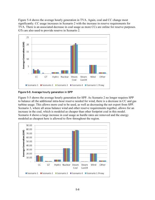
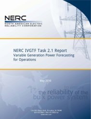
Figure 5-4 shows the average hourly generation in TVA. Again, coal and CC change most
significantly. CC usage increases in Scenario 2 with the increase in reserve requirements for
TVA. There is an associated decrease in coal usage as more CCs are online for reserve purposes.
GTs are also used to provide reserve in Scenario 2.
Figure 5-5: Average hourly generation in SPP
Figure 5-5 shows the average hourly generation for SPP. As Scenario 2 no longer requires SPP
to balance all the additional intra-hour reserve needed for wind, there is a decrease in CC and gas
turbine usage. This allows more coal to be used, as well as decreasing the net export from SPP.
Scenario 3, where all areas balance wind and other reserve requirements together, allows for an
increase in the coal, which is modeled as cheaper than other footprint coal in this model.
Scenario 4 shows a large increase in coal usage as hurdle rates are removed and the energy
modeled as cheapest here is allowed to flow throughout the region.
5-8