OF MAXIMUM FLOODS - WMO

WORLD METEOROLOGICAL ORGANIZATION
TECHNICAL NOTE No. 98
ESTIMATION
OF MAXIMUM FLOODS
Report of a working group of the Commission for Hydrometeorology
WMO -No. 233.TP.126
Secretariat of the World Meteorological Organization • Geneva • Switzerland
1969

© 1969, World Meteorological Organization
NOTE
The designations employed and the presentation of the material in this publication do not
imply the expression of any opinion whatsoever on the part of the Secretariat of the World
Meteorological Organization concerning the legal status of any country or territory or of its
authorities, or concerning the delimitation of its frontiers.
Editorial note: This publication is an offset reproduction of a typescript submitted by the
authors.

PREFACE
The preparation of this Technical Note was an exercise in international collaboration.
The Working Group had been asked to give as many examples from various countries
of the worJ,.d as possible. It was perhaps inevitable that the majority of examples would be
drawn from those countries whose experts were members of the Working Group. The reader will
note, however, that there has been a conscious effort to include references and examples
from other countries as well. It was also inevitable that, for solving some problems, more
than one technique is presented, reflecting procedures and practices in different countries.
It is hoped that the reader will find this an enrichment of the text rather than a complication.
In addition to the official members of the Working Group, there were several
"unofficial" Working Group members who contributed substantially to the Technical Note. .In
particular, Chapter 5 was written by Prof. A. F. Jenkinson, of University College, Nairobi,
Kenya.and Section 4.4 by David Rockwell, Corps of Engineers, U.S. Army, Portland, Oregon,
U.S.A. The members of the Working Group were Mr. R. Arlery (France), Mr. S. BanerJi (India),
Mr. D. J. Bargman (East Africa), Mr. J. P. Bruce (Canada chairman),.Dr. A. G. Kovzel
(U.S.S.R.), Dr. V. Kfiz (Czechoslovakia), Mr. V. A. MYers (U.S.A.).
It is the hope of the WOrking Group that hydrologists and hydrometeorologistsin
many countries will benefit from this summary of techniques, both physical and statistical,
for estimation of design floods.
J. P. Bruce (Chairman)

VI
CHAPTER 6 (continued)
CONTENTS
6.3 Methods of applying probability distributions •..•.•.............•......•..••• 232
6.4 Making use of historical flood data •...•....•••...••••.••.............•.•...• 237
6.5 Analyses for rivers with two flood regimes .•......•..••..... ......•.••..••.•• 239
6.6 Peak discharge probabilities for ungauged locations •.....••.•..... ...••...••• 241
CHAPTER 7 - USES OF METEOroLOGICAL DATA IN ESTIMATING FLOOD FREQUENCIES
7.1
7.2
Introduction ..•.....•......•..••...••....•..••....••.•.•...•..•..•••••......•
Small impervious areas ......................- .
7.3 Multiple influences in streamflow frequencies for natural basins •....•..•....
7.4 Historical series method ....................................... e.••••••••••••••
7.5
7.6
Historical series method for very large basins •.......•••..•.......••••....••
Joint probability method ........................................................
Annexes
I. Procedures Used in U.S.S.R. for Computation of Maximum Discharge of
Snowmelt Floods with Little or No Hydrometric Data ••...••.. ...•.•..•.•••.•••• 269
II. Methods of estimating probable maximum runoff according to the maximum
intensity of precipitation or snowmelt ........•. 281
263
263
263
264
265
266

2 ESTIMATION OF MAXIMUM FLOODS
that if the structure is to last 100 years, the chance of a lOO-year
return period flood occurring within its lifetime is 63%. That is the
lOO-year structure, designed for a lOO-year flood, is designed with a
63% chance that its capacity will be exceeded. Extending the analysis
further, in order to have only a 5% chance that the structure's capacity
. will be exceeded, the engineer must design fora 1950-year return period
flood. The unreliability of estimates of the magnitude of such rare
events by statistical means from relatively short periods of observational
records, and the need for very safe design criteria particularly for
structures which are upstream from populated areas, has led to increasing.
use of physical analyses of design floods. Indeed where earth-fill
construction is used upstream from urban centres, many engineers are of
the opinion that the spillways should be designed to pass the physical
upper limits to flood flows which the basin above the dam site is capable
of producing. The greater part of this Technical Note (chapters 2-4) is
concerned with physical analysis estimates of extreme floods.
Since,. aside from those caused by earthquakes and landslides,
major floods are a result of meteorological conditions, such physical
analyses start with meteorological studies. In all climatic zones this
involves estimation of maximum snow accumulation and melt rates. Where
the rainfall studies are directed towards estimation of the physical upper
limits to storm rainfall in a basin or region, the resulting_estimates
are usually called the "probable maximum storm" or "probable maximum
precipitation". vlhen converted into flood flows by one of the methods
outlined in chapter 4, the resulting flood is known as the "probable
maximum flood". Another, less widely used set of terms is "standard'
project storm and flood". These terms are used to denote the largest

CHAPTER 1
storm that has occurred in a-climatically homogeneous region and is
considered to be reasonably typical of that region, and the flood that
would result if such a storm was centred on a basin _within this region.
A better understanding of the significance of these terms will be obtained
by a study of the methods of estimating the magnitude of these extreme
events and the application of such estimates, as outlined in subsequent
chapters.
Throughout the Technical Note, examples are given from various
parts of the world covering as many of the major climatic zones as proved
feasible.
It should be emphasized that the final selection of design
criteria for any structure involves economic and even moral and political
considerations in addition to those of a hydrologic nature. The job of
the hydrologist and hydrometeorologist is to provide the data and analyses
needed to permit intelligent assessment of the flood potential of the
site in question. It is our hope that this Technical Note will contribute
to an improvement in analysis procedures and practices in the world, and
to a better understanding of the importance of hydrological analyses in
safe and efficient design of river structures.
1.2 Glossary of Terms
A selection of technical terms employed in sections 2.1 to 2.6
is listed below for the convenience of the reader, with either their
corresponding definition or a paragraph reference to a definition found
in the text. In general, the terms defined here are common to all of
meteorology while the terms defined in the text belong primarily to
the specialties of rainfall maximization or analysis.
adiabatic chart - a thermodynamic diagram employed by meteorological services
3

CaAPTER 1 5
isohyet-area graph - a curve derived from an isohyetal chart depicting the
isohyetal values vs. the area enclosed within each isohyet. (2.2.8.5)
lapse rate - the rate at which temperature in the atmosphere changes in
the vertical; either aT/ah or- aT/ap where T is temperature, h height, and
P pressure.
mass curve - a plot of accumulated depth of precipitation at a point or
averaged over a desired area against time. Also see paragraph 2.2.6.
mixing ratio - the dimensionless ratio of mass of water vapor to mass of
dry air with which it is mixed
w = .622
e
p-e
where w is mixing ratio, p atmospheric pressure, e vapor pressure, and
.622 is the ratio of the molecular weight of water to the average molecular
weight of dry air. Also given in gm kg-I, and is then 1000 times above
value. Similar to specific humidity.
moisture maximization - the process of adjusting storm precipitation
upward to a theoretical value that would have pertained if the moisture
content of the air had been at the maximum for the location and season but
other storm conditions had remained unchanged.
precipitable water - the total atmospheric water vapor contained in a
vertical column extending between two specified levels, or if unspecified,
from the surface to the top of the atmosphere. Expressed as the depth of
liquid water of equal mass over an area equal to the cross-sectional
area of the column. Also called liquid equivalent of water vapor.
1
gp f qap
where w = precipitable water, g is acceleration of gravity, q specific
humidity, P pressure, and a density of liquid water. One set of consistent

6 ESTIMATION OF MAXIMUM FLOODS
units fulfilling this formula are cm for w, mb for P, g kg- l
-2 -3
cm sec for g, and gm cm for d
for q,
-2 -3
g = 980 cm sec ,d = 1.0 gm cm
probable maximum precipitation - "The theoretical greatest depth of
precipitation for a given duration that is physically possible over a
particular drainage area at a certain time of year."*
rain profile - a form of isohyet-area graph in which the area enclosed
by an isohyet is replaced by the radius of a circle of equal area. (2.2.8.6)
rawin - a method of measuring upper-air winds by tracking a balloonborne
target \vith radar, or radio direction-finder. Possesses the advantage over
the earlier visual tracking of pilot balloons in that observations are not
limited by clouds or precipitation.
saturation adiabat - a curve on a thermodynamic diagram depicting the
saturation adiabatic lapse rate.
saturation adiabatic lapse rate - the theoretical rate at which the
temperature of a rising saturated air parcel decreases, with the following
assumptions. (1) adiabatic, that is no heat exchange by radiation or
conduction between particle and environment. (2) water vapor in excess
of saturation immediately condenses to liquid. (3) latent heat released
by condensation warms the air. The saturation adiabatic lause rate is
normally closely approximated in clouds of marked vertical development
such as cumulus, cumulonimbus, or deep layers of altostratus.
sequential maximization - reducing the observed elapsed time between
storms to develop a hypothetical severe precipitation sequence. (2.4.1.5)
* from Glossary of Meteorology, American Meteorological Society, Boston,
Nass., USA, 1959.

CHAPTER 1
spatial maximization - reducing the distance between precipitation storms
or storm bursts to develop a hypothetical severe precipitation sequence.
(2.4.1.5).
specific humidity - the dimensionless ratio of the mass of water vapor to
the total mass of humid air.
e
q = .622 P
where q is specific humidity, P atmospheric pressure, e vapor pressure,
and .622 is the ratio of the molecular weight of dry air. Specific humidity
is also given- in g k -1, and is then 1000 times the above value. For most
practical purposes may be interchanged with mixing ratio.
composite maximization - developing hypothetical severe precipitation events
by joing together storms or storm bursts. Comprised of sequential maximiza-
tion and spatial maximization.
storm transposition - moving a storm from its place of occurrence to a basin
under study in representation of a possible future storm at the latter
location.
wet-bulb potential temperature - the temperature an air parcel would have
if cooled dry adiabatically from its initial state to saturation, and thence
brought to 1000 mb. by a saturation-adiabatic process. The wet-bulb potential
temperature is constant along a saturation adiabat, and thereby may be used
as a label for such a curve. Same as 1000-mh. dew point in many hydro-
meteorological writings.
1

2.1 Physical Models of Rainstorms
CHAPTER 2
MAXIMlThi RAINFALL
2.1.1.1 Two rainstorm models are described here, a general
model and a model for orographic rainfall on the windward side of mountain
ranges.
Further details on the first model relating to moisture maximization
of storms are found in chapter 2.4. A list of definitions of terms used in
chapters 2.1 to 2.6 is found in section 2.1.4.
The convergence model
2.1.2.1 The convergence model focuses attention on the following
three properties of precipitation storms: (a) humid air converges quasi­
horizontally toward the storm area; (b) the humid air rises; (c) the humid
air cools by adiabatic expansion, forcing water vapor in excess of saturation
from the gaseous to the solid or liquid form. This general model applies
to all scales of storms from the individual thunderstorm to the large-area
rain associated with a tropical or extra-tropical cyclone.
2.1.2.2 The theoretical interrelationship of convergence,
vertical motion,and condensation is known. To whatever precision either
the convergence at the various levels in -the atmosphere or the vertical
motion should be kno\vn or assumed, averaged over some definite time and
space, the other could be calculated to equal precision from the principle
of continuity of mass. The yield of precipitation by'adiabatic cooling
of air of a certain water vapor content is also knmvn to a high degree
of precision. Observations confirm that the theoretical saturated
9

10 ESTIMATION OF MAXIMUM FLOODS
adiabatic lapse rate of temperature of ascending saturated air from
which precipitation yield is calculated is closely approximated in
deep, precipitating clouds. The higher the specific humidity, the greater
the precipitation yield for a given decrease in pressure. Thus the model
clarifies the concept that intense rainfall over a basin results from the
combination of intense rate of convergence of air (or maximum vertical
motion) and high water vapor content. The extreme rainfall would result
from the extreme combination.
2.1.2.3 There is a problem in estimating maximum
rainfall with th"e convergence model. Maximum water vapor content
of the air can be estimated with acceptable reliability for all
seasons for most parts of the world by appropriate interpretation
of climatological data. But there is neither an empirical nor a
satisfactory theoretical basis for assigning maximum values to either
convergence or vertical motion. Direct measurement of these variables
has been elusive. The solution to this dilemma is to use observed
rainfall as an indirect measure of convergence and vertical motion.
Extreme rainfalls are the indicators of maximum rates of convergence
and vertical motion in the atmosphere. The convergence and vertical
motion are jointly called the precipitation "mechanism".
2.1. 2.4 Extreme "mechanisms" from extreme storms are then
transposed to basins under study without the necessity of calculating
the magnitude of the convergence and vertical motion explicitly.
Rather, the observed rains in storms are adjusted to values over the
basin by attention to the following questions. (a) Can each
observed storm be transposed to the study basin, that is, can the
. .
"mechanism" which produced the storm be shifted to the basin? The

CHAPTER 2
answer to this is found ina synoptic meteorology approach, discussed
in chapter 2.3 on storm transposition. (b) Dpon transposing an
observed storm to the study basin, what is the maximum moisture
content of the air that the transposed mechanism could be expected
to operate upon to produce precipitation? How much would the precip­
itation in these circumstances exceed that observed in the actual
storm? This adjustment is calculated from the phvsics of the moist
adiabatic process and is discussed in chapter 2.4. Cc) Hhat assurance
is there that a maximum "mechanism" has been introduced by this indirect
'process of transposing and adjusting rainstorms? To ensure this, a
sufficient number of intense rainstorms must be transposed and
adjusted to the basin and the resulting adjusted storm rainfall
magnitudes enveloped. The difficult question of what is "sufficient"
is discussed at the end of chapter 2.4.
2.1.2.5 The most simplified technique for carrying
out the process described in the preceding paragraph is to divide
the precipitation in a storm (in tilillimeters) by the precipitable
water in the surrounding air (also in millimeters) and obtain a
dimensionless ratio that is a measure of the efficiency with which
the "mechanism" produces precipitation from water vapor. Various
names have been applied to this ratio. In some reports of the D.S.
Weather Bureau (24),(30), this is called a P/M ratio, standing for
"precipitation/moisture." A "P/H ratio" thus determined is related
to a specific duration, location, and area of the rainfall value
used for IIp''. P/M ratios may be smoothed and enveloped geographically,
seasonally, and over storm duration, to obtain characteristic maximum
values. Multiplication of a maximum ratio of this nature by the
11

CHAPTER 2
(g) Calculate the rate of precipitation generation within the
layer from
where
R
t
R rainfall in centimeters in time t in hours.
V wind speed in km/hr. at inflow.
P depth of layer in millibars at inflow.
x
(2.2)
-1
q ,q = specific humidity of air in gm kg at inflow and outflml7
a e
respectively. q is found from qa on an adiabatic chart by proceeding
e
up a moist adiabatic from the inflow pressure to the outflow pressure
atcenter of the layer.
-2
g acceleration of gravity (980 cm sec).
-3
p density of water = 1.0 gm cm
X horizontal distance from foot to crest of mountain, km. The total
precipitation is the sum of that generated in the several layers.
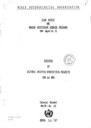
2.1.2.4 Distribution of precipitation along slope. The
calculated distribution of the precipitation along the slope is obtained
by constructing trajectories of the precipitation - rain or snow -
from point of formation down to the ground (figure 2.1). Each segment
of a trajectory is the vector sum of the wind and the assumed terminal
velocity of the raindrop or snowflake* as in figure 2.2. Snow falls
* Terminal velocities vary with raindrop and snowflake dimensions.
Acceptable averages are about 6 meters per second for raindrops
and 1.5 meters per second for snowflakes (24 p. 53-54).
15

SNOW
TERMINAL
VelOCITY
RAIN
TERMINAL
VELOCITY
CHAPTER 2
SNOW
TRAJECTORY
RAIN
TRAJECTORY
Figure 2.2 - Construction of raindrop and snowflake trajectories
17

18 ESTIMATION OF MAXIMUM FLOODS
2.2 Analysis of Storm Rainfall Data
2.2.1 The need for volumetric rainfall data. Rainfall is
measured, and tabulated in the usual climatological records, at
isolated points on the surface of the earth. Floods, however, result
from substantial volumes of rain spread out over a substantial fraction
of a basin or all of it. Thus any appraisal of storm rainfall for the
purpose of estimating flood magnitudes is concerned with rainfall
volumes, expressed as average depths (in millimeters or inches) over
specified sizes of area (in square kilometers or square miles) falling
in specified intervals of time.
2.2.2 Depth-duration-area values. Point rainfall measure-
ments are commonly accepted as presenting the average depth over a
few squalre kilometers. For larger areas,valumetric storm rainfall
values are obtained by an integratic;m of point rainfall values. Usually,
the largest. values of precipitation averaged within selected sizes of
area and in selected durations within a storm are abstracted from the
complete array of such depth-duration-area values (commonly abbreviated
DDA values) and are presented in graphical or tabuclar form as the
principal end product of the analysis.
2.2.3 Treatment of analvsis . of storm rainfall data in
this Note. This section of the Technical Note is restricted to
discussing the p-urposes and characteristics of storm rainfall data
in the DDA. form, as the WMO is issuing a separate manual describing
in detail the procedures for computing such values. The purposes
and characteristics of DDA analyses can be clarified by a review of
some of the history of their development. Certain developments in
the United States of America are reviewed in sections 2.2.4 and 2.2.5

CHAPTEli 2 21
In constructing mass curves for such an analysis, the analyst considers
all possible clues. These clues include comparison with adjacent
recorder mass curves, noting of any times of beginning and ending
of precipitation or miscellaneous corrnnents (such as "rain heaviest
in the afternoon") on observational forms, and weather maps. When
the rainfall can be associated with synoptic features that are
depicted on weather maps, these in turn give clues to the time
distribution of the rainfall 'and progression of rainfall centers
through the storm area. These techniques have been surrnnarized in
a report (22).
One mass curve of figure 2.4 depicts the trace from a
recorder (Cincinnati). The 'other two mass curves, from stations
with daily measurements at 7a.m. and 5.p.m. respectively, are
constructed by taking the recorder chart observation as a guide.
2.2.7 Isohyetal charts
2.2.7.1 Flat terrain. In flat terrain isohyets are
generally drawn smoothly, interpolating between stations. The
interpolation should not be excessively mechanical.
2.2.7.2 Mountainous terrain. In mountainous regions
the simple interpolation technique would yield unsatisfactory isohyets.
Yet to prepare a valid isohyetal pattern in a mountainous region is
not easy. One commonly used procedure is the isopercental technique,
excellent under certain limited conditions stated in the next paragraph.
This method requires a base chart of either mean annual precipitation,
or preferali1.y mean precipitation for the season of the storm, such
as winter r summer, or monsoon months. In this method the ratio qf

28 ESTIMATION.OF MAXIMUM FLOODS
the storm precipitation to the mean annual or mean seasonal precipi­
tation (base precipitation) is plotted at each station. Isolines
are drawn smoothly to these numbers. The ratios on the lines are
then multiplied by the original base chart values at a large number
of points to yield the storm isohyetal chart. Thus the storm
isohyetal gradients and locations of centers tend to resemble the
features of the base chart, which in turn is influenced by terrain.
The first requirement for success of the isopercental
technique is that a reasonably accurate mean annual or mean seasonal
precipitation chart be available as a base. The base chart is of
more value if it contains precipitation stations in addition to
those reporting in the storm than if both charts are drawn exclusively
from data observed at the same stations. The value of the base chart
is also enhanced, in regions where the runoff of streams is a large
percentage of the precipitation, if the precipitation shown on the
chart has been adjusted not only for topographic factors, but also
adjusted to agree with seasonal streamflow. In regions where a
large percentage of the precipitation evaporates adjustment to
runoff volumes would be of dubious value.
An additional requirement for success of the isopercental
technique is that most of the annual or seasonal precipitation in
the region result from storms with relatively the same wind direction,
and from storms with minimal convective activity. Under these
circumstances an individual storm will have a strong resemblance
to the mean chart, as the latter is an average of kindred storms.
In the Tropics with the dominance of convective activity
and with lighter winds, the isopercental technique is of less value

CHAPTER 2
these purposes. The isohyetal chart may be a simple one since its
primary function is to identify the storm location. Routinely
available weather maps may be sufficient to identify the storm causes,
particularly if the precipitation is closely associated with either
a tropical or an extratropical cyclone. In other instances a detailed
analysis may be necessary to identify causes.
In the Tropics it is often difficult to associate
precipitation clearly with features on the available weather maps.
2.3.3.2 Region of influence of storm type. The second
step is to delineate the region in which the meteorological storm
type identified in step I is both common and important as a producer
of precipitation. This is accomplished by survey of a long series
of weather charts. The daily Northern Hemisphere weather charts
(23) are suitable for this purpose over much of the Northern Hemisphere
outside the Tropics. Tracks of tropical and extratropical cyclones
are generally available in published form to indicate the regions
in which these storms are frequent.
2.3.3.3 Topographic controls. The third step is to
delineate topographic limitations on transposability. Coastal
storms are transposed along the coast, but only a limited distance
inland. Inland storms are so placed that major mountain barriers
do not block the inflow of moisture from the sea unless this circum­
stance was present in the original location of the storm. Transposition
behind moderate and small barriers is taken care of by storm adjustment
(see below). Some limitation is placed on latitudinal transposition
in order not to involve excessive changes in air mass characteristics.
37

38
ESTIMATION OF MAXIMUM FLOODS
2.3.3.4 Final step. The final step in transposition is
to apply transposition adjustments discussed in the next section.
Transposition adjustments
2.3.4.1 Moisture adjustment for location. The moisture
available in the atmosphere for production of precipitation is an
'important factor in the maximum precipitation that may be expected
in different regions. The extreme demonstration of this is a
comparison of precipitation in polar regions with tropical regions.
It is customary in transposing storms to apply an adjustment for
moisture. This is derived from charts of enveloping dew point
values, reduced to a common elevation. Such dew point maps are
discussed in section 2.4, on maximization. The dew points are
converted to precipitable water in a saturated pseudo-adiabatic
atmosphere from the ground to some great height by figure 2.9. The
transposition adjustment is then the ratio of the precipitable water
for the enveloping dew point at the transposed location to that
where the storm occurred.
where
r
RI observed precipitation in a storm, for a particular duration
and size of area.
R 2 = precipitation adjusted for transposition.
r transposition adjustment.
W l
precipitable water in a saturated pseudo-adiabatic atmosphere
from ground to some great height, corresponding to maximum
surface dew point at location of storm occurrence.
(1)
(2)

CHAPTER. 2
regions with greater frequency than over adjacent valleys is well
knovTn. Above 1500 meters the decrease in available moisture becomes
over-riding and an elevation adjustment is applied for transposition
based on precipitable water. In making such adjustments, the effective
elevation of the ground at the place of occurrence of the storm and
in the transposed position are employed rather than the precise point
elevations, to allow for the fact that a thunderstorm draws in moisture
from some distance away. The effective elevation is either
the average ground elevation over some tens of square kilometers
surrounding a location, or the average elevation over a specified
sector five to ten kilometers long in the downhill direction only.
4. On broad, gradually sloping plains, such as the Plains region
extending from Texas and Oklahoma northward, the relocation adjust­
ment for transposition is applied as described in paragraph 2.3.4.1
but no explicit additional adjustment for elevation is made. However,
elevation change of more than 700 meters is generally avoided.
Local or regional studies of ·available storm precipitation
should influence any elevation adjustments. For example, it is not
known prior to study of a particular tropical region whether the
most intense precipitation from the deep moist air mass occurs at
low elevations from ready triggering of convection or at higher
elevations from other effects.
2.3.4.6 Climatological adjustments. Other factors besides
topography and moisture effect storm magnitudes. The action of these
factors is suggested by such climatological charts as mean annual
precipitation, maximum observed values of point precipitation, and
heavy rainfall frequency charts. An example of the latter would be
43

CHAPTER 2
theory in constructing frequency maps) and integrates many factors
not all of which can be identified.
2.3.4.8 The recommended procedure for using climatological
charts as guides to transposition is:
(a) Select the climatological chart that is most strongly
influenced by storms of the type to be transposed.
r', from:
(b) Calculate a tentative transposition adjustment ratio,
r' = F IF
2 1
where F l and F 2 are the climatological rainfall values at the location
of storm occurrence and the transposed location, respectively.
(c) Regard r' as the outer limit of the transposition adjustment
and subjectively adjust to a value, r, closer to 1.0 on the basis
of judgment. (Increase r' if less than 1.0, decrease if more than
1.0). The full adjustment, r', would more often be used as a
transposition adjustment to develop some lesser category of design
storm such as "Standard Project" storm than to develop PMP.
Reference distance procedure for moisture adjustment
2.3.4.9 An alternate procedure for moisture adjustment for
relocation to that described in paragraph 2.3.4.1 is to use as an
index of the moisture in a storm, not the observed surface dew points
at the center of the storm, but rather such dew points at some
distance from the storm as much as several hundred kilometers, in
the direction from which the moist air enters the storm. This
procedure is particularly appropriate with winter cyclones. The dew
points are from the warm sector of the cyclone regardless of whether
the precipitation occurs there or, more typically, north of the
(5)
45

CHAPTER 2 47
warm front with cold air at the surface. In this circumstance
the surface dew points near the storm are not representative
of the moisture flowing into the storm. At the transposed location
the same referenced distance is laid out on the same bearing from
the transposition point. This indicates where to scale the maximum
dew points from the maximum dew point chart for calculating the
transposition and maximization adjustment. See Figure 2.10.
Examples of transposition
2.3.5 Figures 2.11 and 2.12 illustrate transDostion
limits applied to storms in the course of studies in the United
States. Included are notes as to the reasons for establishing
the indicated transposition limits. In the study of a particular
basin, it is of course not necessary to establish transposition
limits completely around a storm but only in the direction of
the basin.
2.4 Storm Rainfall Maximization
2.4.1 Introduction
2.4.1.1 There are three princiDal methods of storm rain­
fall maximization: statistical, physical and composite. Statistical
methods are discussed in chapters 5 and 6.
2.4.1.2 Physical Method. rne physical method of maximization
is applied to individual storms and is used in combination with trans­
position and envelopment. References 3, 10, 12, 15, 18, 20 dnd 36
are survey papers which describe this method or some aspect of it.
The physical method is based on the model described in section 2.1.
In that model, the most vital element of a rainstorm is a cloud
system into which air converges radially at lower levels, rises to

CH1l.PTER 2
Explanation of Vigure 2.11
Study Basin
Transposition limits
Northern: Encloses storms' of similar type and
region of high. frequency of nocturnal
thunderstorms.
Eastern: Extent to which inflow can come to
region without crossing higher Appalachian
Hountains.
Hestern: Generalized lOOO-meter elevation contour ­
above which isohyets would reflect
topographic effects
o Center of July 9-13,1951 -storm isohyetal pattern
in place of occurrence.
/ X . Center of major summer storms with all of the following
synoptic and rainfall ch2.racteristics similar to
July 9-13, 1951:
1. East-west frontal and rainfall patterns.
2. No marked wave action or occulsions during
and after rain period.
3. Duration of rain equal or greater than 2 days.
4. Rain at storm center equal" or greater than 7 inches.
5. Polar High to north or rain center during rain
period.
6. Southward movement of frontal system .after rain.
o
( F)---Percent(%): Transposition adjustment iso1ines labeledlvith
enveloping mid-July deH points (OF) and percent (%)
of storm rainfall values of storm in place of occurrence.
4-9

The storm
CHAPTER 2
Explanation of Figure 2.12
A hurricane approaching the D.S. from the southeast
crossed the Coast on the night of the 13th. On the relatively flat
coastal region 13.5 inches of rain over 1000 square miles was
observed in 24 hours. The storm continued in a northwesterly
direction and a day later came against the slopes of the Appalachian
Mountains which rise to about 5000 feet in this region. Here the
rainfall intensified due to orographic lifting resulting in a
second rain center with 15.0 inches in 24 hours over 1000 square
miles. This is one of the most severe rainstorms of record for the
Appalachian Mountains.
Transposition
Hurricanes affect all of the eastern D.S. seaboard and
have been responsible for floods throughout the eastern Appalachians.
The storm under consideration occurred along some of the steepest
and highest eastern slopes and the central isohyets have orientation
and shape that conform to terrain features. Because of this
orographic control, transposition of the storm center is limited
to a rather narrow strip along the eastern slopes.
51

54
ESTIMATION.OF MAXIMUM FLOODS
is permitted and is not restricted to the chronological order of the
original sequence. Spatial maximization consists of reducing the
distanee between simultaneous storm bursts. Obviously spatial and
sequential maximization may be used together, and commonly are.
The hypothetical rearrangements of observed storms or storm bursts
may be useful in assessing possible future storms.
2.4.1.5 Maximization methods applied to floods. It is
interesting to note that floods as well as rainfall are maximized
by the three methods. Statis:ical analysis of flood frequencies is
common (chapter 5). Increasing an observed flood by recomputing the
runoff with a decreased infiltration rate is an example of a
physical maximization. This would be a very suitable maximization
of a flood from heavy rain on ground initially very dry. The
sequential maximization of flood hydrographs is well known, and many
years ago was the intuitive response of engineers confronted with
design problems on rivers. The phasing of the contributions of
tributaries to a main stream in a manner more critical than
actually observed in a flood is also a composite type of maximization
of flood flows.
2.4.2 Moisture maximization
2.4.2.1 Thunderstorms. The most extreme discharge from
basins up to a few hundred sq. km. in area in warm temperature and·
tropical regions will generally result from ore or more thunderstorms.
These extreme thunderstorms, whether isolated or in groups, are
characterized by an inflow of very moist air at low levels which
quickly reaches the· condensation level, rises through clouds along
a moist adiabat to the tro!iopause, and penetrates into the base of

64 ESTIMATION OF MAXIMUM FLOODS
not as great. For comparison, specific humdity differences along
moist adiabats between 900 mb. (1 km.) and 400 mb. (7 km.) are
shown in figure 2.13, curve El, and the relative variation of this
difference in figure 2.14, curve E. However, inflow levels and
outflow levels are less readi1y'specified in this type of storm
than in extreme thunderstorms. Further, in large-area storms
much of the more intense precipitation is frequently the result of
thunderstorms and associated convective activity. In view of the
uncertainties, the U.S. Weather Bureau has applied the precipitab1e
water ratio adjustment of formula (4) to large-area storms as well
as thunderstorms.
2.4.2.8 Orographic storms. The maximization of
orographic storm precipitation by the orographic model of paragraph
2.1.3 is described in section 2.4.7. In maximization by the
orographic model the moisture adjustment is applied implicitly by
processing air along sloping streamlines, each with its own moist
adiabatic temperature variation and its own decrease in pressure
over the span of the windward face of the mountain.
2.4.3 Dew Points
2.4.3.1 Moisture maximizationof a storm requires
identification of two saturation adiabats. One typifies 'the
vertical temperature distribution in the storm to be maximized,
with the greatest weight given the time and place of the heaviest
precipitation. The other is the warmest saturation adiabat that
could be expected in a storm at the same place and season. It is
tBcessary to identify these two saturation adiabats with some
indicator, and the conventional 1ab1e in meteorology for saturation

CHAPTER 2 65
adiabats is the wet-bulb potential temperature. An alternate
identifier is the 1000-mb. dew point. Surface dew points in the
inflowing tropical air in or near a storm identify the storm
saturation adiabat. The moist adiabat corresponding to either
the highest dew point of record at the location and season, or
dew point of some specific return period such as 25 or 50 years,
is considered sufficiently close to the warmest probable saturation
adiabat. Both the storm and maximum dew points from higher elevatioI
stations are reduced to 1000 mb. along the moist adiabat on which
they lie at their respective pressures to obtain the wet-bulb
potential temperature. Ensuring paragraphs give further specifications
on the use of dew points in this manner as the basis for moisture
adjustment of storms.
2.4.3.2 Maximum dew points. Where surface dew point data
are available, a satisfactory method for obtaining the maximum
moisture index is to survey along record at several stations. All
high values for each station are plotted against date and a smooth
seasonal envelope drawn as illustrated in figure 2.15. Monthly
values are then read from these graphs at the 15th day of each
month, adjusted by the saturation adiabatic to 1000 mb. and plotted
m monthly maps. Smooth enveloping isopleths are drawn on the maps.
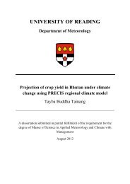
Figures 2.16 and 2.17 show maximum dew point charts constructed in
this way for selected dates in West Pakistan (17) and the United
States (35) .
. 2.4.3.3 Synoptic limitations on maximum dew points. Certain
precautions are advisable in the dew point maximization procedure.
First, the maximum dew point charts are intended to be an index of

30-JUNE
CHAPTER 2
rv
co IS-JULY
HIGHEST PERSISTING 12-HOUR IOOO-MS
DEWPOINTS-DEGREES FAHRENHEIT
Figure 2.16 - Highest persisting 12-hr. lOOO-mb. dew points (oF)
in West Pakistan. Selected dates. From (17).
67

CHAPTER 2
moisture in storms. In certain places and seasons characterized
by ample sunshine, sluggish air circulation, and numerous lakes,
rivers and swamps, a local high dew point may result from local
evaporation of moisture from the surface and not represent a large
volume of a tropical air mass. Such values can be discounted in
constructing the maximum dew point charts. This problem is most
aggravated in the Tropics but it is also present at higher latitudes
in summer, where daily insolation equals tropical values.
2.4.3.4 To control this local modification of dew points,
the analyst inspects the surface weather charts for the dates of the
highest dew points and eliminates those in which the station is clearly
in an anticyclonic or fair weather situation rather than a
cyclonic circulation with tendencies toward precipitation.
2.4.3.5 l2-hr. persisting dew points. Another problem
with high dew points has to do with observational techniques. The
most common method of measuring dew point is with a psychrometer. If
the wet-bulb of this instrument is not sufficiently moistened and
ventilated, its temperature will not be depressed sufficiently below
the dry bulb. A calculated dew point from such contaminated data
is incorrectly high. Assuming such errors are committed only
occasionally, there is merit in basing maximum dew point values
on two or more consecutive observations rather than on a simple
individual reading. The D.S. Weather Bureau uses the highest
persisting 12-hr. dew point, that is the highest value equaled or
exceeded at all observations during 12 consecutive hours. For
example, the following is a series of dew points observed at
6-hour1y intervals. The highest persisting 12-hr. dew point is 24°C.
69

70
ESTIMATION OF MAXIMUM FLOODS
22 23 24 26 24 20 21
2.4.3.6 Average maximum dew points. Another method of
obtaining smoothing in maximum dew points is to average over six
or twelve hours. The maximum average 6-hr. dew point in the above
series is 25.0 0 C (two consecutive observations) while the maximum
average 12-hr. value (3 consecutive observations) is also 25.0 0
C.
2.4.3.7 Single observation maximum dew point. Single
observation dew point maximums may be used as the maximum moisture
index provided the record is examined for dubious values and the
synoptic test of paragraph 2.4.3.3 is applied. These tests should
be applied in any event, but are particularly necessary to appraise
single observation maximum dew points.
2.4.3.8 Storm dew point. To select the saturation adiabat
representing the observed storm moisture, the highest dew points in
the warmest airmass flowing into the storm are identified on surface
weather charts. This determination may be made in the rain area
but not necessarily so. Dew points at stations between the rain
area and the sea should also be considered. This tolerance
is to insure that the dew points are in the warmest airmass involved.
In some storms, particularly storms related to warm fronts, surface
dew points in the rain area may represent only a shallow layer of
cold air and not the temperature distributions in the convective
clouds that are releasing the rain. Figure 2.18 illustrates
schematica11y a weather map on which the storm dew point determination
is made. On each consecutive weather map for the duration of a
storm the maximum dew point is average over several stations as

14
•
16
•
24
•
CHAPTER 2
23
•
24
•
H EAVY RAI N AR.EA
Figure 2.18 - Determination of maximum dew point in a storm.
Representative dew point for this map time is
average of values in boxes
19
•
71

84 ESTIMATION OF MAXIMUM FLOODS
probable maximum precipitation or some less extreme category of
maximum precipitation. Figure 2.19 is an example of such a chart.
Other examples are found in (12).
2.5.1.2 An early example of generalized. charts of areal
values of maximum precipitation specifically for use in spillway
design are those of Bailey and Schneider (1). Highest observed
rains for a selected duration and area ,.;rere plotted on cross
sectional st.rips extending tlIrough the eastern half of the United
States in various directions. Enveloping depth lines were then drawn
on each strip. Cross checks between adjacent strips and smoothing
within strips oriented indifferent directions resulted in smooth
regional envelopes. Transposition of storms was considered only
to the extent of smoothing between highest precipitation points".
This procedure of course yielded lower values than 'l7hat is now called
probable maximum precipitation because storms were not moisture
maximized, and transposition was limited as just described.
2.5.2 Advantages of generalized charts
2.5.2.1 There are several advantages to a generalized
chart approach to maximum precipitation estimates. These are (a)
consistency, (b) thoroughness, and (c) availability. An organization
responsible for design of several comparable projects desires con­
sistency in the design flood from project to project. This is
more readily accomplished if the design floods for individual
projects are related to a generalized nreciuitation chart which
encompasses all of the project sites than if some reliance is on
separate studies for each site made perhaps at different times.
Consistency in itself will not necessarily insure a better value for

98 ESTIMATION OF MAXIMUM FLOODS
undergirded by a study of a number of storms and considering many
factors is required in shaping the PMP isopleths.
2.5.6.5 The separation method. The reports of the D.S.
Weather Bureau (25, 32) describe a separation method of preparing
generalized estimates of PMP. Both observed and probable maximum
storms in the mountains near the Pacific Coast of the United States
are conceived as the combined result of two effects, orographic
precipitation which may be estimated from the orographic model
(par. 2.4.7.4) and "convergence precipitation" from storm processes
not directly resulting from the mountains. The "convergence" part
of the PMP is estimated by moisture maximizing storm values occurring
in relatively flat regions near the mountains. These are then
transposed to the mountains applying an assumed decrease of this
component with elevation. The orographic and convergence components
of the PMP are estimated for a basin separately by use of different
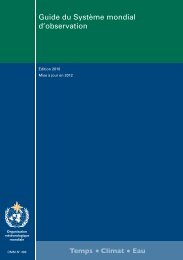
charts and nomograms and then added together for total PMP.
The orographic and convergence components have different seasonal,
areal, geographic, and elevation variations. Figures 2.24 and 2.25
depict portions of index maps of the respective components of 6-hr.
PMP in the state of California, of the D.S.A., from (32). The
different character of the two distributions is evident.
2.5.7
2.5.7.1
Dse of generalized PMP charts
Generalized charts usually provide PlW for one
or more standard duration-area combinations in map form and DDA
relationships to calculate depths -for other standard duration-area
combinations. From these, an array of basin-wide.6-hr. increments
of PMP is obtained.

Figure 2.24
CHAPTER 2 99
- Example 0 f orographie
PMP

100 ESTIMATION OJ!' MAXIMU1VI FLOODS
Figure 2.25 -
Example 0 f convergence
PMP

CHAPTER 2
by one day the intervening time between storms will produce a
significantly greater overlap of the respective hydrographs and
a significantly greater peak flow. Like other factors associated
with design rainstorms, this minimum time interval in a hypothetical
storm sequence is derived by combination of (a) envelopment of
the record - in this case selecting the smallest, not the largest ­
and (b) deduction to what is reasonable from the point of view of
synoptic meteorology.
2.6.2.3 Dual typhoons or hurricanes. In tropical and
subtropical regions subject to frequent typhoons, hurricanes, or
tropical depressions at certain seasons, two of these storms in
sequence should be given consideration as the prototype for a major
flood over a large river basin. Tropical storm tracks are usually
fairly well recorded in available publications. Study of these
tracks may lead to a conclusion as to minimum reasonable time
interval between two storms, or in exceptional circumstances the
interval between heavy rainfalls from the same storm following a
looping track.
2.6.2.4 Hypothetical map sequence technique. The
most rigorous check on a presumed minimum time interval between
two storms and on the overall- synoptic compatibi-lity of the two,
is to construct a series of surface weather charts depicting one
possible evolution of the weather leading from one storm to the
other. This is done in an illustration that follows. Other
illustrations are found in a study of the U.S. Heather Bureau (29).
Once the conviction has been established for a particular
climate or region that hypothetical map sequences connecting certain
103

104
ESTIMATION OF MAXIMUM FLOODS
of the major storm types can be constructed, then verbal descriptions
of synoptic weather developments between storms may suffice to
establish valid sequences. The latter was done in a more recent
study of the U.S. Weather Bureau (28).
2.6.3 Example of storm sequence in middle latitudes
2.6.3.1 The following example of a two-storm sequence at
middle latitudes illustrates some of the factors to be considered
in this type of work. In the example, it is supposed that one is
concerned with heavy flood flows on the portion of the Mississippi
River marked with hatch marks in figure 2.26. Deductions for this
region would be similar to other relatively flat areas in the middle
latitudes with the warm ocean moisture source in rather close
proximity to the south.
2.6.3.2 Flood behaviour. The first task is to
survey past floods, taking note of the seasonal variation and the
contribution of flow by the major tributaries. The largest
contributor tg winter floods on the lower Mississippi River is the
Ohio River. A question to pose and answer is: What flows could
result on the Mississippi if an extreme Ohio River flood were
followed by a.storm centered farther downstream? (Other questions
would be posed regarding spring floods originating over the western
tributaries. The example here will be restricted to a winter
sequence. )
2.6.3.3 Selection of storms. The largest flood of record
on the Ohio River was in January 1937. The rain that produced this
flood is chosen as the firs.t part of the storm sequence. One period
of substantial rains farther downstream begins on January 3, 1950.

112 ESTIMATION OF MAXIMuM FLOODS
The high pressure that follows the first front needs to become
established at a latitude sufficiently far south so that moist
air can eventually be transported northward around its western
periphery from south of 20 o N. To insure that moisture would be
transported from such southerly latitudes a fourth or fifth day
between fronts was needed. Thus a five-day interval is used in the
example here.
2.6.3.8 The first map of the series of figure 2.28 is
the actual morning map for January 25, 1937, while the last is
the actual map for January 3, 1950. The hypothetical maps between
are a synthesis of the actual developments following the 1937
storm and preceding the 1950, and of various movements of weather
features such as high- low-pressure areas and frontal systems
found on other maps. Charts depicting normal movements for various
seasons are also. a useful guide.
2.6.3.9 In the figures of the hypothetical maps solid
arrows depict 24-hr. motions of fronts and centers of Highs and Lows.
Open arrows are successive 24-hr. trajectories of a cold air parcel
and a warm air parcel that find themselves in juxtaposition at the
beginning of the second rainstorm, and illustrate the development
of a strong temperature gradient in the region of the front.
2.6.3.10 Since surface weather maps are available for
a much longer period than are upper-air charts, the surface maps are
emphasized. However, a particular sequence is more firmly established
when the upper levels are considered as well as the surface. In the
present sequence the hypothetical surface charts were tested by
construction of associated hypothetical maps for upper levels.

CH/l.PTER 2 113
Charts of departure-from-normal and day-to-day changes of the
hypothetical surface and upper-level pressures and temperatures
were also constructed.
2.6.4 Flood sequences and probable maximum precipitation.
It should be noted that the example storm sequence above does not
and was not intended to provide a synthetic flood hydrograph comparable
in severity to the "probable maximum precipitation" with which most
of other portions of chapter 2 are concerned. The requirements of
the investigation from which this example is drawn was for a design
flood for levees and relief flood-ways rather than spillways of dams.
The "probable maximum" is difficult to define for large basins because
of the numerous coincidental factors required to produce floods from
large areas. However, a hypothetical sequence can be made to yield
a flood hydrograph approximately comparable to "probable maximum"
by: (1) a combination method well down the list of table 2.6.1;
(2) adequate transposition and maximization of some of the outstanding
events from an adequate sample of major storms; and (3) selecting as
short a time interval between storms as is meteorologically conceivable.

114 ESTIMATION OF MAXIMUM FLOODS
REFERENCE:;
(1) Bailey, S.M., and G. R. Schneider, "The Maximum Probable Flood
and its Relation to Spillway Capacity," Civil Engineering, Vo!. 9,
January, 1939, pp. 32-36.
(2) Battan, Louis, "Radar Meteorology", The University of Chicago
Press, 1959.
(3) Bruce, J.P., "Storm Rainfall Transposition and Maximization",
Proceedings of Symposium No. 1, Spillway Design Floods, at Ottawa,
Canada, November 1959. National Research Council of Canada,
pp. 162-170.
(4) Canada, Department of Transport, Meteorological Branch, "Storm
Rainfall in Canada", Toronto, Ontario. 1961 - (continuing
publication) •
(5) Chow, V.T., "A general formula for hydrologic frequency analysis",
Trans. Amer. Geophysical Union, Vo!. 32, 1951, pp. 231-237.
(6) "Handbook of Applied Hydrology," edited by y,. T. Chow, McGraw-Hill,
New York, 1964, p. 8-23.
(7) Corps of Engineers, U.S. Army, "Storm Rainfall in the United States",
Washington, 1945-.
(8) Court, Arnold, "Area-Depth Rainfall Formulas," Journal of Geophysical
Research, Vol. 66, June 1961, pp. 1823-32.
(9) ESSA-Weather Bureau, Technical Note 3 - NSSL 24, "Papers on
Weather Radar, Atmospheric Turbulence, Sferics and Data Processing."
August 1965.
(10) Fletcher, R.D., "Hydrometeorology in the United States," Chapter in
"Compendium of Meteorology," American Meteorological Society, Boston
U.S.A., 1951, pp. 1033-1047.
(11) Fruhling, A., Ueber Regen- und Abflussmengen fur stadtische
Entwasserungskanale, Der Civilingenieur (Leipzig), ser. 2. Vol. 40,
p. 558, 1894.
(12) Gilman, C.S., "Rainfall", Chapter 9 in "Handbook of Applied Hydrology',
edited by V.T. Chow, McGraw-Hill, New York, 1964.
(13) Hershfield, D.M., "Estimating Probable Maximum Precipitation,"
Journal of Hydraulics Division, Proceedings of American Society of
Civil Engineers, September 1961, pp. 99-116, Separate No. 2933.
(14) Knox, J.B., "Proceedings for Estimating Maximum Possible Precipitation,"
California (U.S.A.) State Department of Water Resources Bulletin
No. 88, 1960.

CHAPTER 2 115
(15) Koelzer, V.A., and M. Bitoun, "Hydrology of Spillway Design Floods:
Large Structures, Limited Data," Journal of Hydraulics Division,
Proceedings of American Society of Civil Engineers, Paper No. 3913,
May 1964, pp. 261-293.
(16) Linsley, R.K., M.A. Kohler, and J.L.H. Paulhus, "Applied Hydrology"
McGraw-Hill Book Co. Inc., New York, 1949, p. 79.
(17) Malik, F.1'1., "Highest Persisting Dewpoints in the Northern Region
of West Pakistan for June through October", Scientific Note, Vol. 16,
No. 1, Dept. of Meteorology and Geophysics, Pakistan, 1964.
(18) Paulhus, J.L.H., and C.S. Gilman, U.S. Weather Bureau,
"Evaluation Probable Maximum Precipitation," Transactions,
American Geophysical Union, Vol. 34, October 1953, pp. 701-708.
(19) Sarker, R.P., "A Dynamical Model of Orographic Rainfall", Monthly
Weather Review (U.S. Weather Bureau), Vol. 94, No. 9, September 1966,
pp. 555-572.
(20) Showalter, A.K., "Quantitative Determination of Maximum Rainfall,"
section in "Handbook of Meteorology", edited by F.A. Berry, E. Bollay,
N.R. Beers; McGraw-Hill, New York, 1945, pp. 1015-1927.
(21) State of Ohio, The Miami Conservancy District, "Storm Rainfall of
Eastern United States," (Revised), Technical Reports Part V,
Dayton , Ohio, 1936.
(22) U.S. Weather Bureau, "Applied Heteorology: Mass Curves of Rainfall,"
1946.
(23) D.S. Weather Bureau, "Daily Series, Synoptic Weather Maps, Northern
Hemisphere Sea Level."
(24) U.S. Weather Bureau, "Generalized Estimates of Maximum Possible
Precipitation over the United States East of the 105th Meridian,
I for Areas of 10, 200, and 500 Square Miles," Hydrometeorological
Report No. 23, 1947, pp. 9-12.
(25) U. S. Weather Bureau, "Interim Report - Probable Maximum Precipitation
in California," Hydrometeorological Report No. 36, 1961
(26) U.S. Weather Bureau, "Manual for Depth-Area-Duration Analysis of
Storm Precipitation;" Cooperative Studies Technical Paper No. 1, 1946.
(27) U.S. Weather Bureau, "Maximum 24-Hour Precipitation in the United
States," Technical Paper No. 16, 1952.
(28) U.S. Weather Bureau, "Meteorology of Flood-Producing Storms in the
Ohio River Basin," Hydrometeorological Report No. 38, 1961.
(29) U.S. Weather Bureau, "Meteorology of Hypothetical Flood Sequences in
the Mississippi River Basin," Hydrometeorological Report No. 35, 1959.

116 ESTIMATION OF MAXIMUM FLOODS
(30) D.S. Weather Bureau, "Probable Maximum Precipitation in the
Hawaiian Islands," Hydrometeoro1ogica1 Report No. 39, 1963.
(31) D.S. Weather Bureau, "Probable Maximum Precipitation, Susquehanna
River Drainage above Harrisburg, Pa.," Hydrometeoro1ogica1 Report
No. 40, 1965.
(32) Weather Bureau, "Probable Maximum Precipitation, Northwest States,"
Hydrometeoro1ogica1 Report No. 43, ESSA, D.S. Department of Commerce,
1966.
(33)
(34)
D. S. Heather Bureau, "Rainfall-Frequency Atlas of the Hawaiian
Islands for Areas to 200 square miles, Durations to 24 Hours, and
Return Periods for 1 to 100 Years," Technical Paper No. 43, 1962.
D.S. Weather Bureau, "Seasonal Variation of the Probable Maximum
Precipitation East of the 105th Meridian for Areas from 10 to 1000
Square Miles and Durations of 6, 12, 24 and 48 hours", Hydrometeoro1ogica1
Report No. 33, 1956.
(35) D.S. Weather Bureau, Sheet of National Atlas of the United
States, "Maximum Persisting 12-Hour 1000-Mb. Dewpoints (OF).
Monthly and of Record," Edition 1960.
(36) Wiesner, G.J., Dept. of Civil Engineering, Dniv. of New South Wales,
Sydney, Australia, "Hydrometeoro1ogy and River Flood Estimation,"
Proc. Institute of Civil Engineers, London, Vol. 27, January 1964,
pp. 153-167.
(37) WMO, "Guide to Hydrometeoro1ogica1 Practices."
(38) WMO, "Design of Hydrologic Networks," Technical Note No. 25, 1958.
(39) WMO, "Use of Ground-Based Radar in Meteorology," Technical Note
No. 27, 1959, Revised 1965.
(40) Wi1son, James W., "Evaluation of Precipitation Measurements with the
WSR-57 Radar," Journal of Applied Meteorology, Vo!. 3, No. 2-,
April 1964.
!I
11
I:
I

3.1 INTRODUCTION
CHAPTER 3
SNOvTMELT CONTRIBUTIONS TO MAXIMUM FLOODS
In high latitudes in many parts of the world, and even at
relatively low latitudes in mountainous regions, major floods are often
a result of melting snowpacks or of snowmelt combined with rain. In
attempting to estimate maximum floods in these regions, it is necessary
to consider the contributions to major floods made by snowmelt water.
solutions to the problem of estimating maximum snowmelt contributions to
floods can be thought of as requiring three steps: (i) determining
maximum seasonal snow accumulations, (ii) estimating critical melting
rates of the snowpack, and (iii) estimation of the percentage of the
melt water- that will appear as streamflow, and its timing. The first
two of these steps are dealt with in this chapter and the third step in
chapter 4. In addition, the question is examined in this chapter of the
critical snowmelt rates that can occur simultaneously or just preceding
or following major rainstorms.
3.2 MAXIMUM SNOW ACCUMULATION
111
Several methods have been used to estimate the upper limits
to snow accumulation on watersheds. These will be referred to as the
Vpartial season method!', I'the snowstorm maximization method", and the
statistical method".
3.2.1 Partial Season Method
One approach to the problem of estimating the physical

120
OUTARDES RIVER--":"-'
BASIN
eNORMANDIN
ESTIMATION OF MAXIMUM FLOODS
/
/'
)
./_..1..-..../
SCALE 20 0 20 40
r=-s==r-.r··,··_··
) MAINE
'---- 1 ------
NEW
BRUNSWICK
-----------.
RIVER
Figure 3.2 - ManicQuagan and Outardes River Basins

CHAPTER 3
of Lake Manuan snowfall. Lake Kanuan data were not assumed to give correct
values for the watersheds in any absolute sense, but it was assumed that the
percentages of greatest observed winter snowfall, obtained by combining
maximum amounts for 4 day, 1 week, fortnight and monthly periods, would likely
be about the same over the watersheds in question as at Lake Manuan. The
percentage of maximum observed winter snowfall (season of 1954-1955) goes
from 125% for the 1 month ':syntbeticIl year to 198% for the 4 day peri.od.
Should one extend this analysi.s to include shorter time periods the percentages
would continue to increase. However, from a study of the frequency of
occurrences of cyclonic storms and the time intervals between theIE in winter
1954-55 and in several other winter seasons of heavy snowfall, a minimum
storm interval of 4 days was accepted.
3.2.2 Snow Storm Maximization Method
The methods of estimating the maximllPJ rainfall that could. have
been produced by a particular storm if the meteorological factors contributing
to precipitation had been most critical have been discussed in Chapter 2.
In short, the procedure involves determination of the ratio of the maximum
moisture conter:t possible at th.at. time of year in the area under consideration,
\
and the actual moisture content of the precipitation - producing air mass in
the storm. The cbserved storm precipitation is multiplied by this maximization
ratio.
In applying the storm maximization procedure to estimating maximum
seasonal snowfall, it is best to select two or more of the greatest snowfall
seasons of record for analysis of individual storms. It is then necessary to
undertake a total storm depth-area analysis within the project basin, for each
significant w'inter storm, by the methcd given in Section 2.2, and to then
determine storm dewpoints and maximization factors as outlined in Section 2.4.
121

CHAPTER 3 123
the calculations when maximum snow water equivalent is considered.
In the snowfall determination in the example used here, the
physical upper limit to snowfall at Lake Manuan would be 200% of the observed
maximum of 630 cm. i.e. 1260 cm. In Canadian snow measurment practise ten
inches (or cm.) of new snow is taken as equivalent to 1 inch (or 1 cm.) of
liquid precipitation. By this procedure, the maximum winter precipitation in
snow would be about 126 cm. water equivalent at Lake Manuan. (The merits of
the ten to one conversion factor are not debated here, but most evidence points
to this factor as being very close to correct on the average over a season in
this part of eastern Canada). Since the mean snowfall over the Outardes is
estimated as being 106% of the mean at Lake Manuan, and over the Manicouagan
basin as being 110% of Lake Manuan snowfall, the physical upper limit of snow­
fall water equivalent over the two basins can be taken as 134 cm. and 140 cm.
respectively.
The results of approaching this problem from a snow cover point
of view are shown in Fig. 3.3. Snow survey measurements of the percentage
water equivalent of the snow pack in the adjacent Lake St. John basin, were
remarkably consistent from place to place and year to year, at the same date.
Curve (1) in Fig. 3.3 represents the maximum percentage water equivalents of
the snowpack at various dates from mid-March on through the snowrnelt season.
These maximum observed values differed only slightly from the mean values.
Curve (2) in Fig. 3.3 illustrates the maximum observed snow depth
on the ground as the snowrnelt season progresses, as a percentage of the seasonal
maximum occurring between March 31 to April 15. This curve was the average
of the maximum percentages at the 3 stations. Nitchequon, Lake Manuan and
Seven Islands, which can be taken to represent reasonably the watersheds in
question. Then by taking the physical upper limit to snow depth as being

3.2.5
CHAPTER 3 125
200% of the-maximum observed, and by applying the snow pack water equivalent
curve (1), the upper curves (3) and (4) in Fig. 3.3 were obtained. They
indicate the physical upper limit to snow pack water equivalent on the
Outardes and Manicouagan basins.
The results obtained by the snowfall and the snow cover approaches
give the maximum snow water equivalent for the Manicouagan as 139 cm. and
142 cm.
As the computations based on snow cover data indicate a maximum
snow pack water equivalent at the end of April, and as rain can occur in
April which would not be considered in the snowfall computations, but which
might well increase the water equivalent of the snm,)' pack by a few inches,
it is to be expected that the snow cover estimates would be slightly higher
than the others. The agreement between the two independent results is thus
remarkably good, and it seems reasonable to accept curves (3) and (4) of
Fig. 3.3 for design flood computations.
Evaluation of Methods
None of these methods are entirely satisfactory. Perhaps the
second approach, by winter snowstorm maximization, is the most soundly based
of the methods, but even here, there is the problem of the compounding of
unlikely events by assuming that all winter storms in a season occur with
maximum water vapour content in the snow-producing air mass. However since
the analyst does not maximize for "mechanical efficiency" of the storm system,
the likely overcompensation for water vapour content may, in part, compensate
for lack of adjustment for storm efficiency. In view of the economic importance,
for optimum design of major dams, of reliable estimates of maximum snm,)'
accumulation, research on new and better methods of making such estimates is
urgently required.

126 ESTIMATION OF MAXIMlThi FLOODS
In some river basins, for example, the Peace River Basin in
British Columbia, where very large storage reservoirs exist or will be created
by dams, it may be that the total spring and summer runoff volume from snmvmelt
is the only criteria involving snow that is required. In these cases the snow
portion of the analysis can be effectively completed by providing estimates of
maximum snow accumulation. However, in most cases, it is important to knmv
not only the total snowmelt volume that can occur but also the timing of the
melt and runoff from the snowpack. In such basins with limited storage,
estimates of critical snowmelt rates are needed to synthesize design flood
hydrographs.
3.3
3.3.1
CRITICAL SNOWMELT RATES
Snowmelt Computation Methods
The approach that is taken to estimating critical snowmelt rates
depends upon the method that will be used to compute these rates and the
meteorological parameters required for that method.
There are two main approaches to computing snow melting rates.
One is the time-honoured degree-day method, and calculate snowmelt runoff by
means of an air temperature index. In this approach the melt "M" in mm. depth
from the snow pack can be expressed as M = C ETa where C is an empirically
determined coefficient and ETa is the sum of positive daily air temperatures
(OC) for a designated period. Either maximum or mean temperatures can be used
for Ta. Such an analysis may not be as naive as it appears at first glance,
for this method has yielded good results for many watersheds. In addition,
there is some physical basis for using a snowmelt temperature index, as air
temperature is reasonably well correlated at a particular time and place with
the atmospheric factors which affect melt rates, such as solar radiation and
vapour pressure, although, it is by no means a perfect index of these factors.

CHAPTER 3
If using the degree-day method, this temperature sequence is all
that is required. However, for the energy balance procedure critical values
of other meteorological factors are needed.
3.3.2.2 Insolation and Albedo.
Clear sky solar radiation represents the upper limit to energy to
be gained by the snowpack by solar radiation. For example, Fig. 3.4 contains
a graph of cloudless day insolation for the Outardes and Manicouagan basins,
based on the work of Mateer (6). However, if rain is assumed to occur con-
current with, or just following, the maximum melt period, insolation values
compatible with rain conditions must be used. In critical snowpack accumulation.-
and melt conditions it could be assumed that snow continues to accumulate until
April 30 in this basin and thus has a high albedo of about 0.8 at the end of
April. The albedo would gradually decrease to about 0.7 as melt progresses
and to 0.4 when the pack becomes shallow, patchy and dirty.
3.3.2.3 Dew Point Temperatures
Except in regions subject to katabatic winds (Fohn winds, chinooks),
where very warm dry air sometimes occurs in winter, the dew point and air
temperature tend to be highly correlated over a melting snow paek. For
example, in the Manicouagan and Outardes basins study, the correlation coefficient
between the two was r = 0.90. The regression equation. relating the two factors
o
was found to be T d = 0.85 Ta - 0.1 (G). Thus, once a critical temperature
sequence is fixed the critical dew point sequence can be directly deduced. If
rain periods are assumed to occur, the assumption can be made that the dew
point equals air temperature.
In regions where snowmelt sometimes occurs with very warm dry
winds, usually downslope winds to the lee of major mountain ranges, it may be
necessary to do separate analyses of dew points for the two types of melt
133

134 ESTIMATION OF MAXIMUM FLOODS
situations under (1) the warm winds and (2) non-downslope wind conditions.
3.3.2.4 Wind
3.4.1
3.4.2
Once high values of insolation have been taken, it becomes in­
consistent to also assume high values of wind, as clear days usually occur
under high pressure conditions with weak surface pressure gradients on the
example used here. a mean daily wind speed of 10 mph was found, from
inspection of Lake Manuan reports, to be as high as one could assume under
such conditions. Under rain conditions different wind limits can be assumed.
By study of winds in spring rainstorms an upper limit of 17 mph as a daily
mean was found to be possible.
3.4 RAIN ON SNOW EVENTS
In many basins the greatest flood will likely result from a
combination of snowmelt and spring rainstorm.
Maximum Rainstorms
The maximum spring storm rainfall can be estimated by the techniques
outlined in Chapter 2, and confining the study to include for maximization
only those storms which have occurred during the critical snowmelt runoff
period.
Snowmelt During Rainstorm
In using the degree-day method, the temperature sequence assumed
to occur during the rain period must be capable of occurrence during a severe
rainstorm in that region, and the degree-day factor "c" must be compatible
with rain conditons. ,This usually means a reduced upper temperature limit
since the highest recorded temperatures are usually under clear skies. To
determine a critical temperature sequence for melt during the rain period, it
is necessary to examine the air temperatures that have accompanied the
controlling spring rainstorms of record. The highest temperatures consistent

CHAPTER 3
with the synoptic conditions occurring in the "design storm" can thus be
assessed.
For the energy balance method, realistic assumptions concerning
dew point temperatures, wind and insolation are required. Estimates of the
first two of these in rain conditions are discussed in para. 3.3.2.3 and 3.3.2.4.
On an overcast day during heavy rain, melt due to short-wave radiation will
be of the order of 0.2 cm/day assuming a snowpack albedo of 0.72 (3). In
addition, under these circumstances there is often a temperature inversion
from the air immediately over the snowpack to the base of the low cloud
layer. In such cases there is likely to be a gain in energy due to
exchanges at long wave lengths rather than the usual loss, and this gain can
o
be estimated by the expression M l(cm) = 1.3 T (C).
r a
REFERENCES
1. Bruce, J.P.
"Snowme1t Contributions to Maximum F100ds lt
Proc. Eastern Snow Conference, pp. 85-103, 1962.
2. WMO Guide to Hydrometeoro10gical Practices, liMO #168. TP. 82, Geneva,
1965.
3. u. S. Corps of Engineers, !'Snow Hydrology" - Summary Report of Snm,
Investigations, June 1956. 433 p.
4. u.S. Corps of Engineers. "Runoff from Snmvme1t" - Engineering and Design
Manual, EM 1110-2-1406, 59 p. Washington, January 1960.
5. U.S. Weather Bureau, Hydrometeoro10gica1 Report #42, Washington, 1966.
135

CHAPTER 4
CONVERSION OF CRITICAL METEOROLOGICAL FACTORS TO FLOOD HYDROGRAPHS
4.1 Statement of Problem
In the preceding chapters, methods of estimating
maximum rainfall, snow accumulation and snowme1t rates have been
discussed extensively. In this chapter techniques are outlined
which permit the analyst to use these meteorological studies in
estimating flood hydrographs at the site of the proposed structure.
There are really two main problems. Given the design rainfall and
snowme1t volumes, what percentage of this total available water
supply will appear almost immediately as surface runoff and
contribute to the flood, that is, what is the runoff volume?
Secondly, how is this total runoff volume distributed in time,
that is, what will be the shape of the flood hydrograph including
the peak discharge?
In classical hydrologic analyses these problems are
treated separately with the runoff volume being estimated first by
means of rainfall (+ snowme1t) - runoff correlations or other means,
and the hydrograph shape being obtained by application of the unit
hydrograph principle. In more recent years, with development of
computer methods in hydrology, these two steps are sometimes not
quite as clearly defined in the analysis. Both classical and
computer approaches to the problem of estimating the design flood
137

138 ESTIMATION OF MAXIMUM FLOODS
hydrograph from input meteorological data are discussed in the
following sections of this chapter.
4.2 Estimation of Runoff Volumes
4.2.1. Introduction. The first step in determining
characteristics of a flood that would result from a given rainstorm
or snowmelt period or both, is to estimate the percentage of the
water on the basin that will appear as surface runoff. Of course,
some of the rain or snowmelt water will infiltrate into the soil
and most of this water will not contribute directly to the flood
rise, but will recharge groundwater and appear as river flow at
a later time or be stored in the soil and used by vegetation.
The water which flows quickly into the stream channels by
mainly overland routes is known as "surface runoff" or "direct
runoff". It is this volume that must be estimated.
4.2.2 Factors Affecting Surface Runoff Volume
It will be recognized that the percentage of rainfall
and snowmelt which becomes surface runoff varies from time to
time within a basin and from basin to· basin. Each basin has a
characteristic response depending on factors such as the
permeability of the soils, the vegetation, the slopes of main
land areas of the basin, the amount of the basin in swamp area
or lakes, and the amount of small depression storage in the basin.
Within a given basin the volumeof surface runoff from a given
amount of rain varies with the season, the antecedent conditions,
and the duration and intensity of storm rainfall.
4.2.3 Rainfall-Runoff Correlations
Since all of these factors are complex and some are

CHAPTER 4
inter-related it is very difficult to estimate runoff volumes
except through use of records of the past response of the river
to incident storm rainfall events or at least records from rivers
of similar characteristics in the same climatic region. For a
particular river basin with records of streamflow and precipitation,
a common procedure is to develop multiple variable rainfall-runoff
correlations. Such correlations may be derived either graphically
or analytically. They usually involve at -least -four variables;
(i) depth of storm rainfall over the basin, (ii) surface runoff
volume from the storm event, (iii) an index of moisture conditions
in the basin prior to the storm and (iv) a seasonal factor. In
some cases storm duration is included as a fifth variable. The
methods of determining these factors from the observational
records in a basin or a region and graphical and analytic
procedures for multiple-variable correlation analyses are outlined
in the \{MO Guide to Hydrometeorological Practices, Annex A,
Wl'vl0 168.TP.82.
An example of storm rainfall-runoff re-lations is given
in Fig. 4.1 for 114 rainfall floods observed at the Valdai Hydro­
logical Research. Laboratory of the State Hydrological Institute
(VNIGL). As the value of the flood runoff depth depends not only
on the depth of precipitation causing the flood but also on the
conditions of the antecedent soil moistening, the precipitation­
runoff relation is expressed not by a straight line, but by a field
of points.
Assuming the precipitation-runoff relation to be linear,
as a first approximation, it is possible to draw several lines
139

CHAPTER 4
a is the runoff coefficient as referred to the excess
precipitation and determined by the slope of the lines.
On determining the H value it is possible to plot the
o
second graph h = f (H - H ) (Fig. 4.2) where this relation is
o
expressed more clearly with a relatively small scatter of points.
In case of availability of several observational stations
within the given geographical zone the parameters of equation (4)
H and a may be defined for all the stations and generalized for
o
the region in a tabular form or by means of an isoline map which
may be applied for adjacent basins with no observational data.
Experience proves that the values H and a are usually
o
stable enough for large climatical regions. For instance, in the
forest zone of the European Part of the USSR the values of H o
vary from 30 - 40 mm at low moistening to 0 - 5 mm at considerable
antecedent moistening, while the corresponding values of a vary
from 0.10 to 0.3-0.4.
The method outlined is a simple and straightforward
technique that permits determination of maximum possible runoff
depth for maximum precipitation amounts in different geographical
zones taking into account antecedent moisture.
4.2.4 Application to Maximum Flood Studies
In applying established rainfall-runoff correlations for
the project basin or for the region in which the basin is located
to estimation of maximum floods certain difficulties arise. The
first is that the range of observed rainfall and runoff volumes from
which the correlations were derived iSffiually not great enough to
141

CHAPTER 4 145
higher than the observed percentage if might be, due to wetter
antecedent conditions and greater rainfall volumes, and adjust
subjectively if a different season of the year is involved. In
the most serious cases of limited data it may be necessar? to
assume a runoff percentage based on experience with severe storms
for similar rivers in the region.
4.3 Time distribution of runoff - unit hydrographs
4.3.1 The solution of many tasks related to water,
management requires determination of hydrograph shape for various
periods. It may be necessary either to assess the discharge
distribution throughout the year as a basis for long-term operations
and water management, or to derive a hydrograph shape for the specific
period of a flood wave to provide criteria for spillway design and
channel improvements and for flood forecasting.
Numerous papers published on this subject bear witness to
the importance of hydrograph shape and indicate at the same time that
techniques are far from being completely definitive. Hydrograph
shape determination for periods of a year or so is still a matter
for basic research and goes well beyond the scope of this Note.
Attention will be given here to determination of time distribution
of runoff in the course of a flood wave.
4.3.2 The methods generally used can be divided into
three groups according to the way in which conditions of the drainage
area are taken into account in order to arrive at a solution.
4.3.2.1 lfuere insufficient data on streamflow are
available to enable the shape of the flood hydrograph to be determined,
it can be approximated by a standard geometrical form. Application

CHAPTER 4 147
curves to derive the wave form of the flood hydrograph. For the
ascending limb he suggested the equation:
·m
Q
x =Q max (_x)
t
l
d for the descending limb:
3
m Is;
where Q is the discharge at time x from the beginning of the
x
flood, Q is the discharge at time z from the peak of the flood,
z
m = Z and n = 3 for rainfall floods, m=n=Z for snowmelt floods,
t l and t z are time bases of the ascending and descending portions
respectively.
Figure 4.3 gives a comparison of waves derived according
to Kotscherin (A) and Sokolowski (B) as shown on the river Ljumes.
Hydrologic investigations of the river Ljumes·in the Albanian -
Yugoslav borderland gave the area of the drainage basin as 520 km.
The maximum discharge given by an areal formula for this region
for p = 1% amounted to 1.650 cu m/so The maximum precipitation
total produced by a single rain storm came to Z50 mm, as estimated
from records of nearest surrounding stations. Assuming a runoff
coefficient of 75% for a flyash soil catchment we obtain (by
analogy with the nearest similar stream) the value of 98 million
cu m for the given drainage area. Then it follows
98 million m 3 •Z
t = hrs = 33.5 hrs.
1,650 m 3 /s 3,600 s
t 1 : t z = 1 : 1. 5
t l = 13.5 hrs: t z = ZO hrs.
Figure 4.1 shows the shape of the simplified waves, which

148
o
0'
LO
.....
ESTIMATION OF MAXIMUM FLOODS
o LO
, ,'"
CIO ......
N.....
co-

CHAPTER 4
gives an approximation to the actual wave shape.
4.3.2.2 It is obvious that simple geometrical forms are
only first approximations and that more attention should be
directed to the characteristics of the drainage area to which
computations are applied. There is no doubt that the individual
waves must differ depending on many influencing factors. For
this reason in a second method the forms were combined with geo­
metrical parameters derived for different typical areas 0 Aleksheyoev
(2) for the territory of the USSR (2).
Kalinin proceeds in a similar way in replacing the
hydrograph by the sume of functions of the two first terms of a
trigonometrical series, and choosing the time of concentration
of the given drainage area as the characteristic parameter. He
determines this value empirically. Apollov and Ogievski (3)
introduce the influence of concentration time into the calculation
and divide the drainage area into smaller areas with constant
time of travel (3) in a manner similar to c.o. Clark (4) in the
U.S.A. Determination of these characteristics by actual
observations is very difficult, and locations where such measure­
ments are available usually allow the introduction of more precise
methods.
The derivations by the different methods mentioned above
are hardly suitable for general use and the description of them
should be taken only as information about ways of proceeding which
might be useful in cases of very limited data. Analyses by these
techniques led the way to later, more reliable, methods of
derivation of the time distribution of runoff.
149

150 ESTIMATION OF MAXIMUM FLOODS
4.3.2.3 Methods based on evaluation of actual observations.
Reliable dataabout stage and discharge, precipitation and other data
concerning basin and precipitation characteristics influencing the
time distribution of runoff are prerequisites for the application
of these methods. These methods are usually reliable enough to
satisfy the exacting demands of most users of hydrologic studies.
This situation creates the need for the establishment and extension
of hydrometeorological networks,· and contributes to a better basic
evaluation of observational data. The hydrologist Voskresenski
draws a fitting picture of the situation: ".••••••..• the way leads
to hydrograph construction based on models derived from generalized
forms of actual floods taking into account physico-geographical
conditions-If. Such models are now widely used.
4.3.2.9 Unit hydrograph method. 'Of all methods of flood
wave form computation, the unit hydrograph method originally presented
by Sherman has been most widely used up to the present time.
It has been subject to modifications by many authors, but of the
basic principles only a few have changed. The term "unit" for
instance is related today to runoff volume, while it referred to
duration in Sherman's original proposals. Many authors called
attention to other problems which in many cases Sherman himself
was aware of. The unit hydrograph is defined, essentially, as a
hydrograph derived from storm rainfall of a specified duration,
where the volume of surface runoff accounted for by this hydrograph
is of unit depth on the basin.
Net rainfall means the portion of precipitation total which
becomes surface runoff. Time of concentration t k is the period

Q
t,
Figure 4.4
Figure 4.5
A·
T
T
Figure 4.6
T
CHAPTER 4 153
T -J-- t
s
-t
Kt.
Kt

CHAPTER 4
equalling 1 x t. we obtain by dividing its ordinates by t., the
. 1 1
unit hydrograph .U for unit rainfall of duration t .• This hydrograph
1 1
should be re-transferred from ordinate scale (expressed in volume
units per time unit) to discharge scale.
This procedure allows transformation of a unit hydrograph of one
duration to one of many other durations for the same drainage area
(Table 4.1). In connection with the second problem (ii) , it must
be taken into account that precipitation of equal duration produces
hydrographs of equal base lengths only if the initial saturation
of the soil and other initial conditions were similar. Soil
saturation and its variations moreover affect the starting point
of the hydrograph rise which usually does not coincide with the .
beginning of rainfall, synchronization being in fact attained only
with initially saturated soil. These difficulties may be overcome
by derivation of unit hydrographs typical not only of specific rain-
fall durations, but also of specified initial conditions. Initial
estimates of net rainfall may be obtained by evaluation ana
comparison of precipitation with corresponding hydrographs under
different initial conditions freely chosen so as to reflect the
character of the given drainage area. A method such as this
was applied in derivation of Table 2 used for the solution of
the following example (3).
Example Derivation of a unit hydrograph is demonstrated for the
drainage area of the brook Modry potok (2.65 sq km) on the uppet
stream of the river Labe, Czechoslovakia.
From observations made in this catchment area 13 rainfalls were
selected of durations that were less than the estimated period of
155

156 ESTIMATION OF MAXIMUM FLOODS
concentration,and corresponding hydrograph rises were determined.
The base flow being almost negligible, separation of base flow
from surface runoff was performed by the straight-line method.
Precipitation values thus obtained were divided into three groups
according to duration of rainfall, taking into account the degree
of saturation of the drainage area at the beginning of precipitation.
Separate hydrographs were derived from precipitation follmving either
continuous dry weather or periods· of heavy rainfall. In this way
hydrographs were obtained for rainfalls of a duration of
t = 3 hrs with antecedent dry period
t = 3 hrs with antecedent wet period
t = 1.5 hrs with antecedent dry period
Fig. 4.7 shows the unit hydrograph for t 3 hrs with antecedent
wet period. Two hydrographs were used for the calculation, volume A
corresponding to 5.71 mm and volume B to 18.1 mm of rainfall. The
s- curve plotted from this unit hydrograph facilitated the construction
of a unit hydrograph for t - 1.5 hrs with antecedent wet period; this
was necessary for plotting of waves derived from several periods of
precipitation.. The derivation is seen on Table 4.1. The observed
data also permitted setting up Table 4.2 as a basis for determination
of net rainfall. The amount of precipitation responsible for runoff
of one mm per time unit is determined for different durations of rain­
fall. Again, alternatives for preceding dry or wet periods were
considered. Table 4.2 serves as an example only and is not applicable
to other drainage areas.
It can be seen that a unit hydrograph may be successfully
employed if we have at our disposal data both on areal and

164
following type -
ESTIMATION OF MAXIMUM FLOODS
Computation and testing programs usually form a regular part of the
library of standard programs for computers. For each hydrograph
basic data in the following categories can be used:
1/ Magnitude of maximum discharge from surface runoff
2/ Time of maximum discharge from the beginning of rainfall
3/ Time of pronounced inflections in the hydrograph from
the beginning of rainfall. These points are best
determined by defining the individual ordinates in
terms of percent of maximum discharge, thus rendering
the individual flood waves comparable.
4/ The value of maximum discharge as well as the abscissas
belonging to the pronounced inflections are considered
dependent variables and assessment should be made of
their dependence upon the independent ones likely to be
responsible for their origin. Independent variables
usually are precipitation duration and precipitation
total, moisture storage in soil, magnitude of low-flow
and me"teorological conditions antecedent to time of
beginning of rainfall.
Testing of the significance of different terms of equations of the
will provide information on the influence of the various factors
upon the formation of the hydrograph rise; the reliability of the
equation can be determined by computation of the coefficients of
multiple correlation and standard error of estimation (13). Equations
of this type were derived for the drainage area of the brook Modry

CHAPTER 4
potok (see application of unit hydrograph, Section 4.3.2.4)
where
Y Qp.m.
vO
- ·p.m.
= 0.010 xl + 0.015 x 4 + 0.419 X s - 0.453
0.306 x 2 - 0.043 x 4 + 2.232 X s + 1.102
0.603 x 2 - 0.0052 x 4 + 6.422 X s +1.482
value of peak discharge from surface runoff
distance of initial point of ·wave from beginning
of rainfall
distance of peak from beginning of rainfall
a precipitation total
duration of rainfall
coefficient of antecedent precipitations
difference of dry- and wet-bulb thermometer
values at time of origin of incident rainfall.
These equations illustrate the effects of individual uarameters in
this particular case. It should be emphasized that the relative
importance of these parameters change with every drainage area.
4.3.2.8 Flood routing
Problems of the time distribution ·of discharge involved
in travel of waves through stream channels and reservoirs forms a
part of a special branch of hydrology. Description of methods used
for flood routing goes beyond the scope of this Note. Mention is
given to them because of their application to reconstruction of time
distribution of discharge for historic floods and for use in analyzing
floods on large drainage basins. For information about publications on
165

CHAPTER 4
4.4.6 Analogue v. Digital Computers. As stated, both
analogue and digital computers have been applied to hydrologic
model simulation. The digital computer, as the name indicates,
performs calculations with numbers expressed by digits. Any
desired degree of precision is attained by using. a sufficient
number of significant figures. An analogue computer applies a
quite different principle. It is designed so that variation in
electric current or voltage simulates (is analogous to) the
variation of some other physical variable such as flow of water.
The analogue output is in graphical rather than digital form.
Because of the wide ranges in capabilities of equipment
and methods of application, only general comparisons can be made
between the two types. The analogue computer is specifically
designed and constructed for a particular task. It then has the
advantage of performing this task immediately and presenting the
result in graphical form. For streamflmv simulation, the digital
computer is often more .practical because it can readily be programmed
to compute any desired hydrologic function. Other advantages are
its availability as a regular commercial item and the fact that it
can be applied to solution of a myriad of-other problems.
4.4.7 Hydrologic Hodel Formulation The computer program is
based on a mathematical hydrologic model which simulates the entire
streamflow process by computation or evaluation of the following
elements: (1) daily (or other period) snmvmelt and/or rainfall
over a sub-basin; (2) losses, either (a) by direct estimate of
transpiration, interception, infiltration, and surface detention,
or (b) indirectly by an antecedent precipitation index, contributing
169

CHAPTER 4
through use of snowrnelt indexes, or rational snowmelt equations
which define the rates of heat transfer to the snowpack, as a
function of meteorologic parameters (see chapter 3).
A computer program can be designed to account for the
relationship between snowpack ablation and decrease of the area
covered by snow. Each day's computed snowmelt is an increment to
the volume of runoff, which in turn is related to the decrease of
snow-covered area. Thus, the computer program maintains a day-to­
day inventory of 1;vater in storage and the -snow-covered area, until
finally the last increment of the snowpack is melted.
Rainfall appropriate to the design flood condition is
added to each day's snowmelt runoff for obtaining the. total water
excess for each day's basin water input. The day's values may be
subdivided into values for shorter periods, 1;vhen required. Evapo­
transpiration loss, soil moisture increase, depression storage and­
deep percolation may be accounted for either directly or indirectly.
The remaining water is then routed to produce the discharge hydro­
graph.
As in the case of rainfall runoff synthesis, snowmelt
coefficients, and basin runoff characteristics can be developed by
the computer model, by reconstitution studies of historical stream­
flow events. The characteristics thus developed are then used
in the computer model for application to design flood conditions.
4.4.17 Summary From the preceding discussion, it ean
be seen that the general approach of streamflow synthesis by
computer provides a means for developing design floods. Because
of the capability of the computer to handle large volumes of input
177

180 ESTIMATION OF MAXIMUM FLOODS
(16)
(21)
(22)
Ke11er, R.
Gewasser und Wasserhausha1t des Fest1andes. Leipzig 1962
(17) Bruce, J.P. and R.H. C1ark
Introduction to Hydrometeoro1ogy. Pergamon Press, Oxford, 1966
(18) Rockwood, David M.
Columbia Basin Streamf10w Routing by Computer, American Society of
Civil Engineers, Transaction Paper No. 3119, 1961
(19) Rockwood, David M.
Program Description and Operating Instructions, 'Streamf1ow Synthesis
and Reservoir Regulation'. Engineering Studies Project 171, Tech.
Bull. No., 22, Jan. 1964. U.S. Army Engineer Division, North Pacific,
Portland, Oregon
(20) Rockwood, David M. and Mark. L,. Nelson
, Computer Application to Streamf10w Synthesis and Reservoir Regulation,
The International Commission on Irrigation and Drainage, 6th Congress,
New Delhi, India, January 1966.
Crawford, N.R., and R.K. Lindsey
The Synthesis of Continuous Streamf10w Hydrographs on a Digital
Computer, Tech. Report No. 12, Dept. of Civil Engineering Stanford
University, Pa10 Alto, Ca1if., U.S.A., 1962
McCa11ister, J.P.
Role of Digital Computers in Hydrologic Forecasing and Analysis,
General Assembly of Berk1ey, Int. Association of Scientific Hydrology,
Vol. 63, pp. 68-76, 1963.

188
220
210
200
180
170
160
150
140
130
120
110
100
90
80
70
fiO
50
40
30
20
10
X
- 1
ESTIMATION OF MAXIMUM FLOODS
0
Fisher - Tippett Type 11
fitted to annual maxima from the. sextiles
x .6.3 + 27.5e.4 y
Type I or Gumbel
fitted by M.L. from 5-year maxima
x x 30.8 + 23.5Y
Type I or Gumbel
fitted by M.L. to annual maxima
x .35 + l6y
Reduced variate V
Figure 5.3 - Annual maximum 24-hour rainfall, Cape Don, Northern Territory
of Australia, 31 years, 1919-1957 (tenths of an inch)
2
3
4
5

26
24
22
20
18
16
14
12
10
8
6
4
X
X
X
CHAPTER 5
Fisher - Tlppett Type I or Gumbel
fitted by M.L. from 5-year maxima
x .10.0 -+- 2.94y
Reduced vari.te Y
- 1 0 2 3
Figure 5.6 - Annual maximum20-day rainfall (inches) at Embu,
Kenya, 46 years, 1914-1962
"
x
5
191

192
5
,
3
2
x
le
x
-, o
ESTIMATION OF MAXIMUM FLOODS
Ftllher - Tippett Type I or ·oumbel
fitted by M.L. from 5-year maxima·
x _ 1.78 + .46y
Reduced variate Y
2 3 5
Figure 5.7 - Annual maximum 24-hour rainfall (inches) for the Chania­
Kimakia catchment, Kenya, 1940-65 Catchment area 160 sq.m.

200
where
-ClL = 1 . Q
ClX
0:;
0
-ClL = 1
{ R - P+Q }
Clk k k
p N -Ee- y
Q
R =
ESTIMATION OF MAXIMUM FLOODS
Ee-y + ky ky
- (l-k)Ep-
-v
N -Ey + Eye J
The computation of the M.L. estimates is illustrated here from the
data for Hartford, Table 5.2 and Fig. 5.2.
· • . .. (21)
· . . .. (22)
We have the first estimate of the parameters made from the
sextiles. The M.L. estimate is obtained by a simple and quick limiting
process. Expression (19) can be put more conveniently for computation
in the forms
ky
e
y
( o:;Jk) /" { (x + 0:;) - X}
o k
= loglO A/0.4343k
For Hartford, starting with k = 0.26;0:; = 3.46; X o
We nmv tabulate the columns
(1) x, noting also the frequencies since the values are grouped;
(2) A = e ky - , . (3) loglO A; (4) y = loglOA/0.4343 k;
These are given in Table 5.3
A
(23)
(24)
(25)
(26)
• • • .• (27)
19.7, A l3.3l/(33.0l-x)

CHAPTER 5 201
Table 5.3- M.L. estimates for flood stage at Hartford. :""irst estimate,
0:= 3.46; x = 19.7; k = 0.26
o .
A=e KY
x frequency = 13.31 loglOA Y = loo- A -v
°10·- e -
33.01-x
.4343 k
12 1 .6335 -.1983 -1. 756 5.789
14 2 .7002 .1548 1.371 3.939
15 4 .7390 .1314 1.164 3.203
16 4 .7825 .1065 .943 2.568
17 3 .8314 .0802 .710 2.034
18 4 .8867 .0523 .463 1.589
19 11 .9500 -.0223 -.198 1.219
20 9 1. 0231 +.0099 +.088 .916
21 21 1.1082 .0446 .395 .674
22 6 1. 2089 .0824 .730 .482
23 8 1. 3297 .1239 1.097 .334
24 3 1.4772 .1695 1.501 .223
25 5 1. 6617 .2205 1.953 .142
26 5 1. 8987 .2785 2.467 .085
27 3 2.2146 .3453 3.058 .047
28 1 2.6567 .4243 3.758 .023
29 1 3.3192 .5210 4.614 .010
30 1 4.4219 .9 456 5.718 .003
I

202 ESTIMATION OF MAXIMUM FLOODS
From the tabulation compute
(1) l:y
(2) l:e- y
(3) l:ye- y
(4) l:e ky
(5)
-y+ky
l:e
Then P = N - (2) = - 0.561
Q = (5) - (1-k)(4) = 0.151
R = N - (1) + (3) = -1.141
Now, if the M.L. solutions are
53.024
92.561
-40.117
1).4.257
84.701
1 1 A 1
0: =0:+0: X =x +x ;k=k+k
000
1 1
where 0:, X O ' k are our initial estimates, and 0: , x o ' are differences
from the M.L. estimates, then we can expand
k) as
1 A 1 A 1
-aL ( 0:- 0: , X - X ' k - k ) in a Tay10r expansion, retaining only
ao:
o o
first and second derivative of -L.
A
A
1 1 1
-aL ( 0:, X k)
0'
= -aL (0:_0: , x x k - k )
ao: ao:
0 0'
0:\_a 2i ) 1 (_a
2
L k
1
(_a
2
= -dL (0:, x k) x ) L ) •••.• (28)
ao:
0' 0
ao:
2 ao:ax ao:ak
0
where the second derivatives are also taken at the M.L. values 0:, x , k.
o
Now since -aL ( 0:, X k) is zero by the definition of M.L. , we have
ao:
0'
1 2
(_a 2 L ) + k 1 (_a 2 0: (-u) + xl L ) = aL ( 0: , x k)
a0:2
0
ao:ax ao:ak ao:
0'
0
From expansions of -aL and -aL we obtain two other equations
ax ak
0
1
( _a
2
L ) + 1 ( _ a 2 L ) + k 1 (_a 2 0: X L ) = aL (0:, X k)
0'
ao:ax
0
ax 2 ax ak ax
0 0 0 0
) = aL (0: , x o ' k)
ak
(29)
. . . .• (30)
..... (31)

For Hartford these are
a: = 3.48
The x,y curve is x
x o
33.17 - 13.49
CHAPTER 5
19.68; k = 0.258
e-· 258 y
The absolute maximum flood stage is estimated.at 33.2 feet; and that for
T = 1000 years is 30.9 feet.
52.3 The Fisher-Tippett TYRe I or Gumbel distribution
As stated in 5.1 the Fisher-Tippett Type I, which has the curvature
parameter kequal to zero, can be regarded as the limit of Type Ill.
The x,y curve is then the straight line of expression (8) viz.
x = x +a:y
o
The straight line has been used extensively for discharges,rainfalls
and other data, advocated mainly by Gumbel, and the distribution is
commonly called the Gumbel distribution. Many references are listed
in Gumbel's book (1958). Other references are· given in Chow (1964).
There was a requirement in July 1966 for an estimate of
extreme rainfall for theChania-Kimakiacatchmentof Kenya; and a
preliminary estimate for 24 hour.rainfall was made, using extreme
value theory, by A.F. Jenkinson, C. Achola and P. Byarugata (unpublished
manuscript, University College, Nairobi). The catchment is situated
at the southern end of the Aberdare range, which extends north-south
for some 50 miles in central Kenya. Some peaks of the range are above
13,000 feet, the general ridge elevation is about 10,000 feet, and
the surrounding lowlands 6,000 feet. The catchment area is about
160 square miles, roughly triangular with apex to the north, and
slopes from 8,000 feet in the south to over 12,000 feet in the' north.
Annual maximum 24 hour rainfall was recorded for each
205

This gives
x - 2.09 = 0.41 (W-O.58)
i.e. x = 1.85 + 0.41 W
Since for k = 0, W = Y we have
x = 1.85 + 0.41 y
i.e. x = 1. 85 and 0:
°
0.41
CHAPTER 5
If we take k 0, the M.L. solution is easily and quickly obtained.
From expression (8) for k = 0 we have that
x - x
y = 0
and we can show that
0:
- dL
dO:
R
0:
- dL = P
dX
0:
0
where P and R are as given in expressions (23) and (25). If we begin
with the estimates
0: =
y
0.41 x o
x - 1. 85
1.41
Then from the tabulations compute
= 1.85 tabulate
(1) Ey; (2) Ee-y; (3) Eye- y
Then P = N - (2); R = N - (1) + (3)
Following a limiting procedure similar to that for the three parameter
1
case, we can obtain new estimates 0: = 0:+0: ;
0:
0:
.65 (-R) + .26(P)
.26 (-R) + 1.11(P)
x o
x o
,,,here
207
• • • •• (37)
• • • •. (38)
(39)
..... (40)
..... (41)

(1) Ey = 15.317
(2) Ee- Y = 26.482
(3) Eye- Y = - 13.362
P = N - (2)
-.482
CHAPTER 5
R = N - (1) + (3) = -2.679
Then from expressions (40) and (41)
Na: 1
a:
= .65(2.679) + .26(-.482) 1.615
Nx 1
o = .26(2.679) + 1.11(-.482) .162
a:
Since a: 0.41 and N 26
a:
1
= (1.615 x .41)/26 = .0255
1
x = (.162 x .41)/26 = .0026
0
So the new estimates fora: and x are
0
A 1
a: = a: +a: .4355
1
x = x + x = 1.8526
000
Repeat the process, starting with these values.
Two steps are usually sufficient.
For the Chania-Kimakia catchment the M.L. estimates, obtained.
at the second step, were
a: = 0.431
The estimates for T
x = 1.852
o
100; 1000; 10,000 years are
x = x + a:y where y has values 4.61; 6.91; 9.31.
o
They are, respectively, 3.83 inches; 4.82 inches; 5.81 inches.
5.3 Confidence Limits
5.3.1 The Gumbe1 case
x = x + Y
o
209

210
and the variance
S 2
x
2
0::
N
ESTIMATION OF MAXIMUM FLOODS
S2 is given, using (42), by
x
or, more formally, using the explicit expressions in the variance-
covariance matrix, (43),
S 2
x
N
1 + i + (1 _ y + y)2
1T 2
S is given in two forms in Table 5.7 for different values of T.
x
Table 5.7 Values of S for the Gumbel line for different
x
return periods T
!"
T Y S
x =
x
JFr
0::
times S = .rn- y times
100 4.61 4.05 .88
1,000 6.91 5.80 .84
10,000 9.21 7.65 .82
100,000 11.51 9.36 .81
00 .78
The form for S given in the last column is probably the easier to
x
use and remember. For T = 10,000 years S = O. 82 0:: Y/ .IN
x
and the multiplier 0.82 can be used for other values of T for
simplicity.
For the Chania-Kimakia catchment annual maximum 24 hour rainfall,
Section 5.2.3, the M.L. estimate
is x = 1.85 + 0.43 y
For T 10,000 years, y 9.31
x = 5.81 inches.
. . •.. (44)
. . . .. (45)

CHAPTER 5
The standard error (S.E.) of estimate is
0.82 ocy /.J"N = 0.82 x 0.43 x 9.31 / m .605 inches
Thus for T 10,000 years
x = 5.81 ± .605 inches
If we adopt the value for T = 10,000 years plus two standard errors
as a reasonable upper limit, this is
5.81 + 1.21 inches + 7.02 inches.
5.3.2 The three-parameter case
From (9) x = x + ocW where W = (l-e-kY)/k W depends only
o
on k for a given y.
Then IX = iX +
o
oc dW
dk
This can be rearranged in themoreo convenient foTm _
+
1
W
dW
dk
211
..... (46)
(Jk) ..... (47)
Then, using the variance-covariance matrix in expression (33)
NS 2
x
2 2
oc W
1
= a + (1:- dW )2
+WZb C +'2. 1 (1. dW)
W dk
W
f
W
dk
(1 dW
2. 1
+ 2 dk )g +
W
h ..... (48)
W
Values of Wand 1 dW are given in Table 5.8 for T
W dk
(y = 6.91) and T= 00
1000 years
The M.L. estimates for Hartford flood stage were given in 5.2.2. The
1 dW
value of k was 0.258. For this value of k, W = 3.22; -==
W dk
Substituting in expression (48) for T = 1000 years
-2.48

218 ESTIMATION OF MAXIMUM FLOODS
Tab1es·9.- N.L. estimation ( k = 0) for the S-year maxima of
flood discharges for the Tana River at Garissa. First estimate
x = 49' er = 18.
o '
Discharge Frequency
x-49 e- y
y =--
18
12.5 1 -2.028 7.599
12.5 5 2.028 7.599
13.3 15 1.983 7.265
16.0 35 1.833 6.253
1Q.3 70 1.817 6.153 ,
17.0 126 1. 778 5.918 I
17.0 210 -1. 778
5.918
18.7 330 -1.683 5.382
18.7 495 1.683 5.382
20.7 715 1.572 4.816
22.8 1001 1.456 4.289
23.8 1365 1.400 4.055
24.5 1820 1. 361 3.900
25.0 2380 1.333 3.792
27.5 3060 1.194 3.300
30.4 3876 1.033 2.809
31.1 4845 .994 2.702
31.1 5985 .994 2.702
32.8 7315 .900 2.460
36.6 8855 .689 1.992
42.2 10626 .378 1. 459
I

CHAPTER 5
48.0 12650 -.056
52.0 14950 +.167
53.0 17550 .222
61.0 20475 .667
63.5 23751 .806
110.0 27405 3.389
1
Then N a: / a:
Total N = 169,911
Ey = 83,875
Ee- Y = 200,154
Eye- Y = -117,000
P = N - Ee- Y = -30,243
R = N - Ey + Eye- Y = -30,964
a:
-.65 R + .26 P
= -.26R + 1.11 P
Since N 169,911 a: = 18
1
a: = 1.30
1
x o
12,263
-25,519
=2.70
Then our new estimates for a: and x
o
are
a: 18 + 1.30 19.30
x
o
= 49 -2.70 = 46.30
The M.L. estimates, obtained at the second step, are
a: = 18.92
So the 5-year maxima are given by
x = 46.41 + 18.92 y
x = 46.41
o
1.058
.846
.801
.513
.447
.034
We can obtain the equivalent I-year maxima from the expressions
a:(l-year) = a:(5-year)
5
x (I-year) = x (5-year) - a:10g
o 0 e
x (5-year) - 1.609a:
o
219
}
}
} . . . .. (50)

220 ESTIMATION OF MAXIMUM FLOODS
N.B. This is a special case of the 3-parameter changes, where the
S-year maxima
x(S-year) A - 11
-ky
e
0:
o:/k )
(writing x +-= A 11
0 k
correspond to the I-year maxima
x(l-year) = A - 11' Sk e-ky
So for Garissa, the equivalent annual maxima are given by
x = (46.41 - 1.609 x 18.92) + 18.92 Y
i.e. x = lS.97 + 18.92 Y
This line is drawn on Fig. 5.1
The discharge with return period T = 1000 years, Y
146.7 cfsx 1000; with S.E•
• 840:
IN
y
= .84 x 18.92 x 6.91
JTI
19.7
6.91 is
We have in fact used all our original' 31 annual maxima to derived
the simulated set of S-year maxima, and so it seems reasonable
to take N = 31 in the expression for the S.E. For T = 10,000 years
x = 192.1 cfsxlOOO with S.E. 2S.9. If we take as an acceptable
"upper limit" the value for T = 10,000 years plus two standard
errors, this is 244.0 cfs x 1000.
A warning should be given against fitting a Gumbel
line by M.L. to the original annual maxima. This would have given
x = 21.2 + 12.86 Y
This line is also drawn on Fig. S .1. It would grossly underestimate
the possible extremes.
To emphasize the warning, Gumbel M.L. estimates from the
• • • •• (SI)

CHAPTER 5
annual maxima are also drawn on Figs. 5.3 and 5.5 for comparison
with the Gumbel M.L. lines for the 5-year maxima. In these cases
also there would be serious underestimation of the possible extremes
for all return periods > T 100.
The M.L. estimates for the 5-year maxima have been drmvn
on Figs. 5.2 to 5.7. For flood stages at Hartford, Fig. 5.2, the
estimated upper limit obtained from the 5-year maxima is the same
as that from the annual maxima, viz 33.2 feet.
M.L. estimates from annual maxima
x = 33.2 - l3.5e-· 26y
M.L. estimates from 5-year maxima
x = 33.2 - l4.le-· 28y
5.4.3 Empirically derived distribution of extremes
Boldakov (1967) stressed that annual maximum flood
discharges should have an upper limit QMM; and he gave an
empirical estimate of this upper limit
l 2
Q = Q (1 + 9.1 C • )
MM v
where Q is the mean of the annual maxima, and C is the coefficient
v
of variation i.e. standard deviation/mean.
He also gave an empirically derived table connecting Q MM
with the upper 10% of the annual maximum flood discharges. A brief
extract is given in Table 5.10.
5.4.4 Relation between maximum catchment rainfall and maximum flood
discharge
Embu, whose annual maximum 20-day rainfall is analysed in
221
(52)

CHAPTER 5
16. P. Gui110t and D. Duband, 1967. La methode de Gradex pour le
ca1cu1 de la probabi1ite des crues a partir des precipitations.
(Paper presented at the International Symposium on Statistical
Hydrology, Fort Co11ins, September 1967)
APPENDIX 5.1 Values of F(x) and y = -log log (l/F)
00
0 1 2 3 4 5 6 7 8 9
_ co -1.53 1.36 1.25 1.17 1 •.10 1.03 0.98 0.93 0.88
10 0.83 0.79 0.75 0.71 0.68 0.64 0.61 0.57 0.54 0.51
20 0.48 0.44 0.41 0.39 0.36 0.33 0.30 0.27 0.24 0.21
30 0.19 0.16 0.13 0.10 0.08 0.05 -0.02 1:0.01 0.03 0.06
40 0.09 0.11 0.14 0.17 0.20 0.23 0.25 0.28 0.31 0.34
50 0.37 0.40 0.42 0.45 0.48 0.51 0.55 0.58 0.61 0.64
60 0.67 0.70 0.74 0.77 0.81 0.84 0.88 0.92 0.95 0.99
70 1.03 1.07 1.11 1.16 1.20 1.25 1.29 1.34 1. 39 1.45
80 1.50 1.56 1.62 1.68 1. 75 1.82 1.89 1.97 2.06 2.15
90 2.25 2.36 2.48 2.62 2.78 2.97 3.20 3.49 3.90 4.61
F(x) y F(x) Y F(x) Y
.005 -1.67 .975 3.68 .991 4.71
.010 -1.53 .980 3.90 .992 4.82
.015 -1.43 .985 4.19 .993 4.96
.020 -1.36 .990 4.61 .994 5.11
225

CHAPTER 6 247
TABLE 1
Corresponding values S = f(C s ) of the coefficient of asymmetry Cs and the
coefficient of skewness S of the binomial curve (according to Alekseyev)
C
s
x -x-
pi
S
x

248
ESTTIVlATION OF MAXIMUM FLOODS
TABLE 1
(continued)
3.6 1.93 -0.42 -0·56 2.48 0.89
3·7 1.91 -0.42 -0·54 2.45 0.90
3.8 1.90 -0.42 -0·53 2.43 0.91
3·9 1.90 -0.41 -0·51 2.41 0.92
4.0 1.90 -0.41 -0·50 2.40 0.92
4.1 1.99 -0.41 -0.49 2.38 0.93
4.2 1.88 -0.41 -0.48 2.36 0.94
4.3 1.87 -0.40 -0.47 2.34 0.94
4.4 1.86 -0.40 -0.46 2.32 0.95
4.5 1.85 -0.40 -0.45 2.30 0.96
4.6 1.84 -0.40 -0.44 2.28 0.97
4.7 1.83 -0.40 -0.43 2.26 0.97
4.8 1.81 -0.39 -0.42 2.23 0.98
4.9 1.80 -0.39 -0.41 2.21 0.98
5. 0 1.78 . -0.38 -0.40 2.18 0".98
5. 1 1.76 -0.38 -0.39 2.15 0.98
5.2 1.74 -0.37 -0.38 2.15 0.98
11
I
I
I
I
II I
I
I

CHAPTER '6
TABLE 5
The Ostravice in FrYdek. Calculation of the curve of the interval
of recurrence of the annual maxiinum discharges for the period
1940 - 1945 including the peaks from 1880 and 1902
",Q
m Year m./ /s
p %*
1880 1000 1,15
1902 920 2,74
1 1940 610 6,32
2 1960 540 9,91
3 1958 500 13,5
4- 1949 440 17,1
5 1959 357 20,7
· · · ·
· · · .'
· · · ·
· · · ·
24 1962 71 89,1
25 '1957 67 92,7
26 1963 52 96,3
I
* for the first historical flood according to the formula (3c), for the
second one according to (3d) and for the other members according to (3e).
x + x - 2x
S = 5 95 90 _ 0,64
x 5 - x 95
x _162 ;;/s
50
s
C = --.!. - 0,906
v
x
C = 2,3
n
253

CHAPI'ER 6
TABLE 6
Annual maximum discharges in the river Pra for the period 1944 - 1960
Q
Month Year
m
m Occurrence tn3; s p = n+l
1 7. 1960 1280 5,57
2 7. 1957 1020 11,14
3 7. 1953 990 16,70
4 9. 1947 810 22,30
5 1l. 1955 780 27,85
6 6. 1958 780 33,40
7 6. 1956 744 39,00
8 10. 1951 720 44,50
9 7. 1944 660 50,10
10 7. 1949 660 55,70
11 9. 1952 577 61,20
12 10. 1959 550 66,80
13 10. 1945 504 72,40
14 6. 1948 504 78,00
15 7. 1954 504 83,50
16 10. 1946 420 89,00
17 10. 1950 262 94,60
255
• 100

CHAPTER 7
basin. Uext the frequency distribution of maximum discharge
is worked out as a function, not of time, but of rainfall. For
example, on a given basin a dai..ly rainfall of lOa nun can be
expected to product a range of maximum discharges on different
occasions, depending on the prior wetness of the soil and other
factors. Tlus span of discharges can be expressed as a fre­
quency distribution, corresponding to 100 mm of rai.11.. Other
frequency distributions are obtained for other quantities of
rainfall. To develop the rainfall-discharge relationships, the
simultaneous period of record of discharges Cind precipitation is
used if it exists; if not, it is necessary to transpose relation­
ships from adjacent basins. Finally, by combining the rainfall
frequency distribution of peak discharges is obtained in terms
of mean recurrence interval.
Generating the discharge vs. rainfall relationships will
usually require a good deal of judgment in treatment of a limited
amoUnt of data.
The indirect procedure is justifiedratl1er than direct
statistical analysis of the discharge record where the precipitation
record exceeds the discharge record in number of years, as is often
the case. An example of application of the joint probability method
is given by Guillot and Duband (5).
267

ANNEX 2
q o,c,g
=----0
(F + C)n
where o _ coefficient taking into account the decrease of maximum spe­
(11 )
cific discharges due to the influence of lakes, swamps, for­
ests and other factors.
On the basis of formula (11) it is possible to write
q
o,c,g
=
qmax,o (F + C)n
0
or in the absence of accumulating factors in the basin ( 0 = 1.0) and accept­
ing C = 1.0 as a first approximation, it is possible to obtain the following:
q = q t (F + l)n
o,c,g max, u
Formula (13) provides an estimate of the values of maximum specific runoff
for comparison with the observed maximum speclfic discharges at hydrological
stations and with the theoretical values of q estimated by the meteoo,c,g
rological method.
8. The comparison shows that the maximum values of specific runoff from
slopes caused by snowmelt q estimated by formula (13) at n = 0.25 aco,c,
cording to the long-term observations of springsnowmelt maxima on therivem
of the USSR, including several thousands of station-years j5j7, are usually
within the limits of q = 2.0 - 3.0 m 3 /sec/km 2 (in the absence of faco,c
tors causing maximum runoff accumulation and considerable smoothening of
floods in flood plains and lower reaches of rivers).
q o,c
pite
In this case, the extreme value of the specific snowmelt runoff
= 3.6 m 3 /sec/km 2 , estimated by formula (5), was never exceeded, des­
the availability of historical spring snowmelt maxima in the given
observation series, with a probable frequency of once every 100-300 years.
Higher values of specific runoff caused by snowmelt reaching q =
max,c
4.0-4.5 m 3 /sec have occurred in some river basins of the mountainous regions
(12)
(13)
285