Smoking adjoints: fast Monte Carlo Greeks - Mathematical Institute

Cutting edge l
The efficient calculation of price sensitivities continues to be among
the greatest practical challenges facing users of Monte Carlo methods
in the derivatives industry. Computing Greeks is essential to hedging
and risk management, but typically requires substantially more computing
time than pricing a derivative. This article shows how an adjoint formulation
can be used to accelerate the calculation of the Greeks. This method
is particularly well suited to applications requiring sensitivities to a large
number of parameters. Examples include interest rate derivatives requiring
sensitivities to all initial forward rates and equity derivatives requiring
sensitivities to all points on a volatility surface.
The simplest methods for estimating Greeks are based on finite difference
approximations, in which a Monte Carlo pricing routine is rerun multiple
times at different settings of the input parameters in order to estimate
sensitivities to the parameters. In the fixed-income setting, for example,
this would mean perturbing each initial forward rate and then rerunning
the Monte Carlo simulation to re-price a security or a whole book. The
main virtues of this method are that it is straightforward to understand and
requires no additional programming. But the bias and variance properties
of finite difference estimates can be rather poor, and their computing time
requirements grow with the number of input parameters.
Better estimates of price sensitivities can often be derived by using information
about model dynamics in a Monte Carlo simulation. Techniques
for doing this include the pathwise method and likelihood ratio method,
both of which are reviewed in chapter 7 of Glasserman (2004). When applicable,
these methods produce unbiased estimates of price sensitivities
from a single set of simulated paths, that is, without perturbing any parameters.
The pathwise method accomplishes this by differentiating the evolution
of the underlying assets or state variables along each path; the
likelihood ratio method instead differentiates the transition density of the
underlying assets or state variables. In comparison with finite difference
estimates, these methods require additional model analysis and programming,
but the additional effort is often justified by the improvement in the
quality of calculated Greeks.
The adjoint method we develop here applies ideas used in computational
fluid dynamics (Giles & Pierce, 2000) to the calculation of pathwise
estimates of Greeks. The estimate calculated using the adjoint method is
identical to the ordinary pathwise estimate; its potential advantage is therefore
computational, rather than statistical. The relative merits of the ordinary
(forward) calculation of pathwise Greeks and the adjoint calculation
can be summarised as follows: a) the adjoint method is advantageous for
calculating the sensitivities of a small number of securities with respect to
a large number of parameters; and b) the forward method is advantageous
for calculating the sensitivities of many securities with respect to a small
88 RISK JANUARY 2006 ● WWW.RISK.NET
Price sensitivity
Smoking adjoints: fast
Monte Carlo Greeks
Monte Carlo calculation of price sensitivities for hedging is often very time-consuming.
Michael Giles and Paul Glasserman develop an adjoint method to accelerate the calculation.
The method is particularly effective in estimating sensitivities to a large number of inputs,
such as initial rates on a forward curve or points on a volatility surface. The authors apply the
method to the Libor market model and show that it is much faster than previous methods
number of parameters. The ‘small number of securities’ in this dichotomy
could be an entire book, consisting of many individual securities, so long
as the sensitivities to be calculated are for the book as a whole and not for
the constituent securities.
The rest of this article is organised as follows. The next section reviews
the usual forward calculation of pathwise Greeks and the subsequent section
illustrates its application in the Libor market model. We then develop
the adjoint method for delta estimates, and extend it to applications such
as vega estimation requiring sensitivities to parameters of model dynamics,
rather than just sensitivities to initial conditions. We then extend it to
gamma estimation. We use the Libor market model as an illustrative example
in both settings. Lastly, we present numerical results that illustrate
the computational savings offered by the adjoint method.
Pathwise delta: forward method
We start by reviewing the application of the pathwise method for computing
price sensitivities in the setting of a multi-dimensional diffusion
process satisfying a stochastic differential equation:
( ) + ( () ) ()
dX̃ t a X̃ t dt b X̃ t dW t
()= ()
The process X ~ is m-dimensional, W is a d-dimensional Brownian motion,
a(·) takes values in R m and b(·) takes values in R m × d . For example, X ~ could
record a vector of equity prices or – as in the case of the Libor market
model, below – a vector of forward rates. We take (1) to be the risk-neutral
or otherwise risk-adjusted dynamics of the relevant financial variables.
A derivative maturing at time T with discounted payout g(X ~ (T)) has price
E[g(X ~ (T)], the expected value of the discounted payout.
In a Monte Carlo simulation, the evolution of the process X ~ is usually
approximated using an Euler scheme. For simplicity, we take a fixed time
step h = T/N, with N an integer. We write X(n) for the Euler approximation
at time nh, which evolves according to:
( )= ( )+ ( ( ) ) + ( ( ) ) ( + ) ( )= ( )
X n+ 1 X n a X n h b X n Z n 1 h, X 0 X̃
0
where Z(1), Z(2), ... are independent d-dimensional standard normal
random vectors. With the normal random variables held fixed, (2) takes
the form:
( )= n ( ( ) )
X n+ 1 F X n
with F n a transformation from R m to R m .
The price of the derivative with discounted payout function g is estimated
using the average of independent replications of g(X(N)), N = T/h.
(1)
(2)
(3)

Now consider the problem of estimating:
the delta with respect to the jth underlying variable. The pathwise method
estimates this delta using:
∂
g( X̃ ( T)
)
X
the sensitivity of the discounted payout along the path. This is an unbiased
estimate if:
that is, if the derivative and expectation can be interchanged.
Conditions for this interchange are discussed in Glasserman (2004), on
pages 393–395. Convenient sufficient conditions impose some modest restrictions
on the evolution of X ~ and some minimal smoothness on the discounted
payout g, such as a Lipschitz condition. If g is Lipschitz, it is
differentiable almost everywhere and we may write:
Conditions under which X ~ i (T) is in fact differentiable in X~ i (0) are discussed
in Protter (1990), on page 250.
Using the Euler scheme (2), we approximate the pathwise derivative
estimate using:
with:
Thus, in order to evaluate (4), we need to calculate the state sensitivities
∆ ij (N). We simulate their evolution by differentiating (2) to get:
i
( )=∆ ( )+ ∑ ∆ kj ( nh ) + ∑ ∑
∆ n+ 1 n
ij ij
⎡ ∂
⎤
E ⎢ g( X̃ ∂
( T)
) ⎥ = E⎡g X̃ T
⎣⎢
∂ X j( 0) ⎦⎥
∂ X j(
0)
⎣
m
∂
g X̃ T X̃ g( X̃ i T
( T)
) = ∑
X 0 X̃ T X̃
0
∂ ( )
∆ ( n)=
ij
m
∂
X
∂ ( )
m ∂ g( X( N)
)
∑ ∆ ij ( N)
∂ X ( N)
i=
1
∂a
∂x j 0
∂ ( )
j 0
∂ Xi( n)
∂ X ( 0)
k = 1 k
ℓ=
1k
= 1
with a i denoting the ith component of a(X(n)) and b iℓ denoting the (i, ℓ)
component of the b(X(n)).
We can write this as a matrix recursion by letting ∆(n) denote the m ×
m matrix with entries ∆ ij (n). Let D(n) denote the m × m matrix with entries:
a
D n
x h i
ik ( )= ik + ∂
δ +
∂
k
i
j
( ̃ ( ) )
E⎡ ⎣
g X T
∂ ( )
∂ ( )
j i=
1 i
, i, j = 1,...,
m
where δ ik is one if i = k and zero otherwise. The evolution of ∆ can now
be written as:
( )= ( )∆( )
∆ n+ 1 D n n
∂biℓ
Zℓ( n+ 1)
h
∂x
with initial condition ∆(0) = I where I is the m × m identity matrix. The matrix
D(n) is the derivative of the transformation F n in (3). For large m, propagating
this m × m recursion may add substantially to the computational
effort required to simulate the original vector recursion (2).
Libor market model
To help fix ideas, we now specialise to the Libor market model of Brace,
Gatarek & Musiela (1997). Fix a set of m + 1 bond maturities Ti , i = 1, ... ,
m + 1, with spacings Ti + 1 – Ti = δi . Let L ~ i (t) denote the forward Libor rate
d
∑
ℓ=
1
( )
d
k
m
⎤
⎦
∂bi
∂x ∂ ( )
∂ ( )
ℓ
k
( ( ) )
j
∆ ( n)
kj
⎤
⎦
Z n+ 1 h
ℓ
( )
(4)
(5)
1. Structure of the matrix D and its transpose
⎛1
⎞ ⎛1
⎞
⎜
⎜
⎜
D =
⎜
⎜
⎜
⎜
⎜
⎝
⎜
1
1
×
×
×
×
×
×
×
×
×
⎟
⎟
⎟
⎟
⎟
,
⎟
⎟
⎟
× ⎠
⎟
⎜
⎜
⎜
T
D =
⎜
⎜
⎜
⎜
⎜
⎜
⎝
1
1
× ×
×
×
×
×
⎟
⎟
⎟
×
⎟
⎟
× ⎟
⎟
× ⎟
× ⎠
⎟
× is a non-zero entry, blanks are zero
fixed at time t for the interval [T i , T i + 1 ), i = 1, ... , m. Let η(t) denote the
index of the next maturity date as of time t, T η(t) – 1 ≤ t < T η(t) . The arbitrage-free
dynamics of the forward rates take the form:
dL̃ i t
= L̃ i t dt i dW t t Ti i m
L̃ ()
t ( ) µ + σ () ≤ ≤ =
T
, 0 , 1,...,
i
()
()
where W is a d-dimensional standard Brownian motion under a risk-adjusted
measure and:
i σi σ jδ jL̃ j t
µ i Lt ̃
()
( () ) =
+ δ L̃ () t
∑
T
1
Although µ i has an explicit dependence on t through η(t), we suppress
this argument. To keep this example as simple as possible, we take each
σi (a d-vector of volatilities) to be a function of time to maturity:
(6)
as in Glasserman & Zhao (1999). However, the same ideas apply if σi is
itself a function of L ~ σi()= t σi− η()+1
t ( )
(t), as it often would be in trying to match a volatility
skew.
To simulate, we apply an Euler scheme to the logarithms of the forward
rates, rather than the forward rates themselves. This yields:
0
( )= ( ) ( ( ( ) ) −
( ) )
= ( )
Li n+ 1 Li n exp ⎡µ
⎣ i L n
2 ⎤ T
σi / 2 h+ σi
Z n+ 1
⎦
h ,
i η nh ,. ..,m
Once a rate settles at its maturity it remains fixed, so we set L i (n + 1) =
L i (n) if i < η(nh). The computational cost of implementing (7) is minimised
by first evaluating the summations:
i σδ j jLj n
Si( n)=
∑ , i = η(
nh) ,..., m
j= η(
nh)
1+
δ jLj( n)
This then gives µ i = σT iSi and hence the total computational cost is O(m)
per time step.
A simple example of a derivative in this context is a caplet for the interval
[Tm , Tm + 1 ) struck at K. It has a discounted payout:
⎛ m 1 ⎞
⎜∏
0
⎝ 1
⎟ δmmax
, L̃ m( Tm)−K δ L̃ T ⎠
i=
0 + ( )
i i i
j= η()
t
{ }
We can express this as a function of L ~ (Tm ) (rather than L ~ (Ti ), i = 1, ... , m)
by freezing L ~ i (t) at L~ i (Ti ) for t > Ti . It is convenient to include the maturities
Ti among the simulated dates of the Euler scheme, introducing unequal
step sizes if necessary.
Glasserman & Zhao (1999) develop (and rigorously justify) the application
of the pathwise method in this setting. Their application includes
the evolution of the derivatives:
( )
j j
(7)
(8)
WWW.RISK.NET ● JANUARY 2006 RISK 89

Cutting edge l
which can be found by differentiating (7). In the notation of (5), the matrix
D(n) has the structure shown in figure 1, with diagonal entries:
and, for j ≠ i:
∆ ( n)=
ij
Dii ( n)=
Li( n+
) Li n i ih
Li( n)
iLi n
+
⎧1
⎪
2
⎨ 1 ( + 1)
σ δ
⎪
2
⎩⎪
( 1+
δ ( ) )
⎧
T
Li n+ 1 σi σ jδ jh
⎪
2
Dij ( n)=
⎨ ( 1+
δ jLj( n)
)
⎪
⎩⎪
0
The efficient implementation used in the numerical results of Glasserman
& Zhao (1999) uses ∆ ij (n + 1) = ∆ ij (n) for i < η(nh), while for i ≥η(nh):
( )
( )
Lin+ 1
∆ ij ( n + 1)=
∆ ( n)+ L ( n+
1)
σ
L n
i
∂ Li( n)
∂ L ( 0)
j
( )
, i = 1,..., m, j = 1,...,
i
i j η nh
> ≥ ( )
otherwise
σδ k kh∆ kj(
n)
( 1+
δkLk(
n)
)
T
ij i i ∑ i
2
k η nh
= ( )
i η nh
< ( )
η( )
i ≥ nh
The summations on the right can be computed at a cost that is O(m) for
each j, and hence the total computational cost per time step is O(m 2 ) rather
than the O(m 3 ) cost of implementing (5) in general.
Despite this, the number of forward rates m in the Libor market model
can easily be 20–80, making the numerical evaluation of ∆ ij (n) rather costly.
To get around this problem, Glasserman & Zhao (1999) proposed faster
approximations to (5). The adjoint method in the next section can achieve
computational savings without introducing any approximation beyond that
already present in the Euler scheme.
90 RISK JANUARY 2006 ● WWW.RISK.NET
Price sensitivity
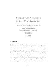
2. Data flow showing relationship between
forward and adjoint calculations
X(0) X(1)
V(0) V(1)
X(N – 1) X(N)
D(0) D(1) D(N – 1)
...
...
V(N – 1) V(N)
g, ∂g/∂X
Guidelines for the submission of technical articles
Risk welcomes the submission of technical articles on topics relevant to our
readership. Core areas include market and credit risk measurement and management,
the pricing and hedging of derivatives and/or structured securities, and
the theoretical modelling and empirical observation of markets and portfolios.
This list is not an exhaustive one.
The most important publication criteria are originality, exclusivity and relevance
– we attempt to strike a balance between these. Given that Risk technical
articles are shorter than those in dedicated academic journals, clarity of
exposition is another yardstick for publication. Once received by the technical
editor and his team, submissions are logged, and checked against the criteria
above. Articles that fail to meet the criteria are rejected at this stage.
Articles are then sent to one or more anonymous referees for peer review. Our
referees are drawn from the research groups, risk management departments and
trading desks of major financial institutions, in addition to academia. Many have
already published articles in Risk. Depending on the feedback from referees, the
Pathwise delta: adjoint method
Consider again the general setting of (1) and (2) and write ∂g/∂X(0) for
the row vector of derivatives of g(X(N)) with respect to the elements of
X(0). With (4) and (5), we can write this as:
∂g
X 0
∂g
∂ ( ) = ∆( N)
∂ X( N)
∂g
= D( N −1)
D( N − 2) ⋯D(
0)∆( 0)
∂ X( N) T
= V ( 0) ∆( 0)
where V(0) can be calculated recursively using:
T
( )= ( ) ( + ) ( )=
V n D n V n 1, V N
⎛ ∂g
⎞
⎜
⎝ X N
⎟
⎠
∂ ( )
(9)
(10)
The key point is that the adjoint relation (10) is a vector recursion whereas
(5) is a matrix recursion. Thus, rather than update m 2 variables at each
time step, it suffices to update the m entries of the adjoint variables V(n).
This can represent a substantial saving.
The adjoint method accomplishes this by fixing the payout g in the initialisation
of V(N), whereas the forward method allows calculation of pathwise
deltas for multiple payouts once the ∆(n) matrices have been
simulated. Thus, the adjoint method is beneficial if we are interested in
calculating sensitivities of a single function g with respect to multiple
changes in the initial condition X(0) – for example, if we need sensitivities
with respect to each X i (0). The function g need not be associated with
an individual security; it could be the value of an entire portfolio.
Equation (10) is a discrete adjoint to equation (5) in the same way that
the differential equation –dv/dt = A T v is the adjoint counterpart to du/dt =
Au, where u and v are in R m and A is in R m × m . The terminology ‘discrete
adjoint’ is used in computational engineering (Giles & Pierce, 2000), but
in the computational finance context it might also be referred to as a ‘backward’
counterpart to the original forward pathwise sensitivity calculation
since the adjoint recursion in (10) runs backward in time, starting at V(N)
and working recursively back to V(0). To implement it, we need to store
the vectors X(0), ... , X(N) as we simulate forward in time so that we can
evaluate the matrices D(N – 1), ... , D(0) as we work backward as illustrated
in figure 2. This introduces some additional storage requirements,
but these requirements are relatively minor because it suffices to store just
the current path. The final calculation V(0) T ∆(0) produces exactly the same
result as the forward calculations (4)–(5), but it does so with O(Nm 2 ) operations
rather than O(Nm 3 ) operations.
To help fix ideas, we unravel the adjoint calculation in the setting of
the Libor market model. After initialising V(N) according to (10), we set
technical editor makes a decision to reject or accept the submitted article. His decision
is final.
We also welcome the submission of brief communications. These are also
peer-reviewed contributions to Risk but the process is less formal than for fulllength
technical articles. Typically, brief communications address an extension
or implementation issue arising from a full-length article that, while satisfying
our originality, exclusivity and relevance requirements, does not deserve fulllength
treatment.
Submissions should be sent to the technical team at technical@
incisivemedia.com. The preferred format is MS Word, although Adobe PDFs are
acceptable. The maximum recommended length for articles is 3,500 words, and
for brief communications 1,000 words, with some allowance for charts and/or formulas.
We expect all articles and communications to contain references to previous
literature. We reserve the right to cut accepted articles to satisfy production
considerations. Authors should allow four to eight weeks for the refereeing process.
T

3. Structure of the matrix B and its transpose
⎛
⎞ ⎛
⎜
⎜
⎜
B =
⎜
⎜
×
⎜ ×
⎜
⎜ ×
⎝
⎜ ×
×
×
×
×
× ×
⎟
⎟
⎟
⎟
⎟
,
⎟
⎟
⎟
⎠
⎟
⎜
⎜
⎜
T
B =
⎜
⎜
⎜
⎜
⎜
⎝
⎜
× is a non-zero entry, blanks are zero
V i (n) = V i (n + 1) for i < η(nh) while for i ≥η(nh):
( ) ( + )
( )
Li n+ 1 Vi n 1
Vi( n)=
+
L n
i
The summations on the right can be computed at a cost that is O(m),
so the total cost per time step is O(m), which is better than in the general
case.
This is an example of a general feature of adjoint methods; whenever
there is a particularly efficient way of implementing the original calculation
there is also an efficient implementation of the adjoint calculation.
This comes from a general result in the theory of algorithmic differentiation
(Griewank, 2000), proving that the computational complexity of the
adjoint calculation is no more than four times greater than the complexity
of the original algorithm. There are various tools available for the automatic
generation of efficient adjoint implementations, given an
implementation of the original algorithm in C or C++ (see Automatic Differentiation
website, www.autodiff.org).
In practical implementations, the payout evaluation may be performed
by separate code or scripts to that used to perform the Monte Carlo path
calculations. In such cases, it may be inconvenient or impractical to differentiate
these to calculate ∂g/∂X(T) and a more pragmatic approach may
be to use finite differences to approximate ∂g/∂X(T) and then use this to
initialise the adjoint pathwise calculation.
Pathwise vegas
The previous section considers only the case of pathwise deltas, but similar
ideas apply in calculating sensitivities to volatility parameters. The
key distinction is that volatility parameters affect the evolution equation
(3), and not just its initial conditions. Indeed, although we focus on vega,
the same ideas apply to other parameters of the dynamics of the underlying
process.
To keep the discussion generic, let θ denote a parameter of F n in (3).
For example, θ could parameterise an entire volatility surface or it could
be the volatility of an individual rate at a specific date. The pathwise estimate
of sensitivity to θ is:
∂ ( )
∂ ( )
∂
∂ =
m g ∂g
XiN ∑
θ X N ∂θ
i=
1
T m σi δih
2 ∑
( 1+
δiLi(
n)
) j= i
If we write Θ(n) for the vector ∂X(n)/∂θ, we get:
Fn
Fn Θ( n + )= X n Θ n
X
X n
DnΘ n Bn
∂
( ( ) ) ( )+
∂
∂
1 , θ
∂θ
( ) , θ
= ( ) ( )+ ( )
i
L n+ 1 V
( )
(11)
with initial conditions Θ(0) = 0. The sensitivity to θ can then be evaluated
as:
j
× × × × ⎞
× ×
×
× ⎟
⎟
× ⎟
×
⎟
⎟
⎟
⎟
⎟
⎠
⎟
( )
j
( )
n + 1 σ j
∂
∂ =
g ∂g
θ X N
∂g
=
X N
where V(n) is the same vector of adjoint variables defined by (10).
In applying these ideas to the Libor market model, B becomes a matrix,
with each column corresponding to a different element of the initial
volatility vector σ j (0). The derivative of the ith element of F n (X n ) with respect
to σ j (nh) is:
∂( )
∂ ( ) =
Fn
i
σ nh
where Si is as defined in (8). This has a similar structure to that of the matrix
D in figure 1, except for the leading diagonal elements, which are now
zero. However, the matrix B is the derivative of Fn (Xn ) with respect to the
initial volatilities σj (0), so given the definition (6), the entries in the matrix
B are offset so that it has the structure shown in figure 3.
From (12), the column vector of vega sensitivities is equal to:
T
⎛ ∂ ⎞ N −1
g
T
⎜ ⎟ = ∑ Bn ( ) Vn ( + 1)
⎝ σ 0 ⎠
The ith element of the product B(n) T V(n + 1) is zero except for 1 ≤ i ≤
N – η(nh) + 1, for which it has the value:
where i* ≡ i + η(nh) – 1. The summations on the right for the different values
of i* are exactly the same summations performed in the efficient implementation
of the adjoint calculation described in the previous section.
Hence, the computational cost is O(m) per time step.
Pathwise gamma
The second-order sensitivity of g to changes in X(0) is:
where:
∂ (
Θ(
N)
)
∂ (
{ B( N −1)+
D( N −1)
B( N − 2)+ ... + D( N −2)
... D()
1 B(
0)
}
)
N −1
∑
= V n+ 1 B n
n=
0
j
T
( ) ( )
⎧ Li( n+ 1)
σδ i iLi( n) h
⎪
⎪
1+
δiLi(
n)
⎪
⎪
+ ( Sh i − σih+
Z( n+ 1) h)
Lin+ 1
⎪ Li( n+ 1)
σδ i jLj( n) h
⎨
⎪ 1+
δ jLj( n)
⎪0
⎪
⎪
⎪
⎩
⎪
( S * h− σ * h+ Z( n+ 1) h L n V n
i i ) * ( + 1) * ( + 1)
i i
δ * L * ( n) h m
i i + ∑ L j ( n+ 1) Vj( n+
1) σ j
1+
δ L ( n)
*
∂ g
X 0 X 0
∂ ( )∂ ( ) = ∑
∂ X ( N)
Differentiating (3) twice yields:
2
m
∂ ( )
* *
i i
Γ ijk
∂g
j k i=
1 i
2
Xin j k
∂ ( )
( n)=
∂ X ( 0)∂ X ( 0)
( )= ∑ ( ) ( )+ ∑ ∑ ( )∆ ℓj(
)∆ mk(
)
Γ n+ 1 D n Γ n E n n n
ijk iℓ
ℓjk iℓm ℓ=
1 ℓ=
1m=
1
where D iℓ (n) is as defined previously, and:
+
m
m
j= i
m
m
( N)
∂ g
X N X N
∑∑ ∆ ij ( N)∆ ℓk
( N)
∂ ( )∂ ( )
i=
1 ℓ=
1
n=
0
i
Γ
ijk
2
m
ℓ
( )
i j η nh
= ≥ ( )
> ≥ ( )
i j η nh
otherwise
(13)
WWW.RISK.NET ● JANUARY 2006 RISK 91

Cutting edge l
For a particular index pair (j, k), by defining:
Gin Γ ijk n , Cin Eiℓmn ℓj
n mk n
this may be written as:
E ( n)=
im ℓ
2
∂ Fi( n)
∂ X ( n)∂ X ( n)
ℓ=
1m=
1
( )= ( ) ( )+ ( )
Gn+ 1 DnGn Cn
m
( )= ( ) ( )= ∑ ∑ ( )∆ ( )∆ ( )
This is now in exactly the same form as the vega calculation, and so the
same adjoint approach can be used. Option payouts ordinarily fail to be
twice differentiable, so using (13) requires replacing the true payout g with
a smoothed approximation; this is the subject of current research.
The computational operation count is O(Nm 3 ) for the forward calculation
of L(n) and ∆(n) (and hence D(n) and the vectors C(n) for each index
pair (j, k)) plus O(Nm 2 ) for the backward calculation of the adjoint variables
V(n), followed by an O(Nm 3 ) cost for evaluating the final sums in
(12) for each (j, k). This is again a factor O(m) less expensive than the alternative
approach based on a forward calculation of Γ ijk (n).
Numerical results
Since the adjoint method produces exactly the same sensitivity values as
the forward pathwise approach, the numerical results address the computational
savings given by the adjoint approach applied to the Libor market
model. The calculations are performed using one time step per Libor
interval (that is, the time step h equals the spacing δ i ≡δ, which we take
to be a quarter of a year). We take the initial forward curve to be flat at
5% and all volatilities equal to 20% in a single-factor (d = 1) model. Our
test portfolio consists of options on one-year, two-year, five-year, sevenyear
and 10-year swaps with quarterly payments and swap rates of 4.5%,
5.0% and 5.5%, for a total of 15 swaptions. All swaptions expire in N periods,
with N varying from one to 80.
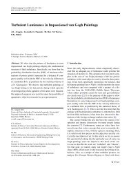
Figure 4 plots the execution time for the forward and adjoint evaluation
of both deltas and vegas, relative to the cost of simply valuing the
swaption portfolio. The two curves marked with circles compare the forward
and adjoint calculations of all deltas; the curves marked with stars
compare the combined calculations of all deltas and vegas.
As expected, the relative cost of the forward method increases linearly
with N, whereas the relative cost of the adjoint method is approximately
constant. Moreover, adding the vega calculation to the delta calculation
substantially increases the time required using the forward method, but
92 RISK JANUARY 2006 ● WWW.RISK.NET
Price sensitivity
4. Relative CPU cost of forward and adjoint
delta and vega evaluation for a portfolio of
15 swaptions
Relative cost
40
35
30
25
20
15
10
5
Forward delta
Forward delta/vega
Adjoint delta
Adjoint delta/vega
0
0 20 40 60 80 100
Maturity N
ℓ
m
m
this has virtually no impact on the adjoint method because the deltas and
vegas use the same adjoint variables.
It is also interesting to note the actual magnitudes of the costs. For
the forward method, the time required for each delta and vega evaluation
is approximately 10% and 20%, respectively, of the time required
to evaluate the portfolio. This makes the forward method 10–20 times
more efficient than using central differences, indicating a clear superiority
for forward pathwise evaluation compared with finite differences
for applications in which one is interested in the sensitivities of a large
number of different financial products. For the adjoint method, the observation
is that one can obtain the sensitivity of one financial product
(or a portfolio) to any number of input parameters for less than the cost
of the original product evaluation.
The reason for the forward and adjoint methods having much lower
computational cost than one might expect, relative to the original evaluation,
is that in modern microprocessors, division and exponential function
evaluation are 10–20 times more costly than multiplication and addition.
By reusing quantities such as L i (n + 1)/L i (n) and (1 + δ i L i (n)) –1 , which have
already been evaluated in the original calculation, the forward and adjoint
methods can be implemented using only multiplication and addition, making
their execution very rapid.
Conclusions
We have shown how an adjoint formulation can be used to accelerate the
calculation of Greeks by Monte Carlo simulation using the pathwise method.
The adjoint method produces exactly the same value on each simulated
path as would be obtained using a forward implementation of the pathwise
method, but it rearranges the calculations – working backward along
each path – to generate potential computational savings.
The adjoint formulation outperforms a forward implementation in computing
the sensitivity of a small number of outputs to a large number of
inputs. This applies, for example, in a fixed-income setting, in which the
output is the value of a derivatives book and the inputs are points along
the forward curve. We have illustrated the use of the adjoint method in the
setting of the Libor market model and found it to be fast – very fast. ■
Michael Giles is professor of scientific computing at the Oxford
University Computing Laboratory. Paul Glasserman is the Jack R
Anderson professor at Columbia Business School. The research was
supported in part by NSF grant DMS0410234. Email:
giles@comlab.ox.ac.uk, pg20@columbia.edu,
REFERENCES
Brace A, D Gatarek and M Musiela, 1997
The market model of interest rate dynamics
Mathematical Finance 7, pages 127–155
Giles M and N Pierce, 2000
An introduction to the adjoint approach to design
Flow, Turbulence and Control 65, pages 393–415
Glasserman P, 2004
Monte Carlo methods in financial engineering
Springer-Verlag, New York
Glasserman P and X Zhao, 1999
Fast Greeks by simulation in forward Libor models
Journal of Computational Finance 3, pages 5–39
Griewank A, 2000
Evaluating derivatives: principles and techniques of algorithmic differentiation
Society for Industrial and Applied Mathematics
Protter P, 1990
Stochastic integration and differential equations
Springer-Verlag, Berlin