Calculating Intermolecular Charge Transport Parameters in ...
Calculating Intermolecular Charge Transport Parameters in ...
Calculating Intermolecular Charge Transport Parameters in ...

Create successful ePaper yourself
Turn your PDF publications into a flip-book with our unique Google optimized e-Paper software.
A thesis entitled<br />
<strong>Calculat<strong>in</strong>g</strong> <strong>Intermolecular</strong> <strong>Charge</strong> <strong>Transport</strong><br />
<strong>Parameters</strong> <strong>in</strong> Conjugated Materials<br />
James Kirkpatrick<br />
Submitted for the degree of Doctor of Philosophy<br />
of the University of London<br />
Imperial College of Science, Technology and Medic<strong>in</strong>e<br />
February 2007
Contents<br />
1 Introduction 4<br />
1.1 Why is a Theoretical Study of <strong>Charge</strong> <strong>Transport</strong> Necessary to the Design<br />
of Better Devices? . . . . . . . . . . . . . . . . . . . . . . . . . . . . . . 4<br />
1.2 Conjugated Materials . . . . . . . . . . . . . . . . . . . . . . . . . . . . 6<br />
1.3 <strong>Charge</strong> <strong>Transport</strong> <strong>in</strong> Conjugated Materials . . . . . . . . . . . . . . . . . 8<br />
2 Background 17<br />
2.1 Marcus Theory <strong>in</strong> the Non-Adiabatic High Temperature Limit . . . . . . 18<br />
2.2 Reorganisation Energy . . . . . . . . . . . . . . . . . . . . . . . . . . . 24<br />
2.3 Transfer Integral . . . . . . . . . . . . . . . . . . . . . . . . . . . . . . . 26<br />
2.3.1 Note on Systems with Degenerate Orbitals . . . . . . . . . . . . 28<br />
2.3.2 Splitt<strong>in</strong>g of the Molecular Orbitals . . . . . . . . . . . . . . . . . 29<br />
2.4 Site Energy Difference . . . . . . . . . . . . . . . . . . . . . . . . . . . 30<br />
2.4.1 Electrostatic Interactions <strong>in</strong> Molecules . . . . . . . . . . . . . . . 31<br />
2.4.2 Inductive Interactions <strong>in</strong> Molecules . . . . . . . . . . . . . . . . 35<br />
2.5 The Gaussian Disorder Model and Related Methods . . . . . . . . . . . . 36<br />
2.5.1 Computational Methods . . . . . . . . . . . . . . . . . . . . . . 37<br />
2.5.2 Distribution of <strong>Parameters</strong> of the Transfer Rates . . . . . . . . . . 40<br />
2.5.3 Predictions and Results . . . . . . . . . . . . . . . . . . . . . . . 43<br />
2.6 Conclusions . . . . . . . . . . . . . . . . . . . . . . . . . . . . . . . . . 46<br />
3 Development and Verification of Methods for <strong>Calculat<strong>in</strong>g</strong> <strong>Charge</strong> <strong>Transport</strong><br />
<strong>Parameters</strong> 53<br />
3.1 Projective Method for Calculation of Transfer Integrals . . . . . . . . . . 54<br />
i
3.2 Molecular Orbital Overlap Method for Calculation of Transfer Integrals . 57<br />
3.3 Calculation of Site Energy Difference from Electrostatic Interactions . . . 59<br />
3.3.1 Ethylene: Neutral Systems . . . . . . . . . . . . . . . . . . . . . 61<br />
3.3.2 Ethylene: <strong>Charge</strong>d Systems . . . . . . . . . . . . . . . . . . . . 66<br />
3.3.3 Pentacene . . . . . . . . . . . . . . . . . . . . . . . . . . . . . . 70<br />
3.4 Comparison of Different Methods of <strong>Calculat<strong>in</strong>g</strong> Transfer Integrals . . . . 73<br />
3.4.1 Pentacene . . . . . . . . . . . . . . . . . . . . . . . . . . . . . . 73<br />
3.4.2 Hexabenzocoronene . . . . . . . . . . . . . . . . . . . . . . . . 78<br />
3.5 Conclusion . . . . . . . . . . . . . . . . . . . . . . . . . . . . . . . . . 82<br />
4 Reorganisation Energy <strong>in</strong> PolyPhenylenev<strong>in</strong>ylene: Polaron Localisation 85<br />
4.1 Introduction . . . . . . . . . . . . . . . . . . . . . . . . . . . . . . . . . 86<br />
4.2 Defect-free PPV . . . . . . . . . . . . . . . . . . . . . . . . . . . . . . . 89<br />
4.3 Torsional Defects <strong>in</strong> PPV . . . . . . . . . . . . . . . . . . . . . . . . . . 92<br />
4.4 Conclusion . . . . . . . . . . . . . . . . . . . . . . . . . . . . . . . . . 94<br />
5 Ambipolar <strong>Transport</strong> <strong>in</strong> PCBM 98<br />
5.1 Introduction . . . . . . . . . . . . . . . . . . . . . . . . . . . . . . . . . 98<br />
5.2 Transfer Integrals . . . . . . . . . . . . . . . . . . . . . . . . . . . . . . 99<br />
5.3 Reorganisation Energy . . . . . . . . . . . . . . . . . . . . . . . . . . . 101<br />
5.4 Monte Carlo Simulations . . . . . . . . . . . . . . . . . . . . . . . . . . 103<br />
5.5 Conclusion . . . . . . . . . . . . . . . . . . . . . . . . . . . . . . . . . 108<br />
6 <strong>Charge</strong> <strong>Transport</strong> <strong>Parameters</strong> for Randomly Oriented Pairs of Dialkoxy Poly-<br />
paraphenylenev<strong>in</strong>ylene and Triarylam<strong>in</strong>e Derivatives 111<br />
6.1 Dialkoxy PPV Series . . . . . . . . . . . . . . . . . . . . . . . . . . . . 112<br />
6.1.1 Introduction . . . . . . . . . . . . . . . . . . . . . . . . . . . . . 112<br />
6.1.2 Method . . . . . . . . . . . . . . . . . . . . . . . . . . . . . . . 116<br />
6.1.3 Results and Comment . . . . . . . . . . . . . . . . . . . . . . . 118<br />
6.2 Spiro L<strong>in</strong>ked Triarylam<strong>in</strong>e Derivatives . . . . . . . . . . . . . . . . . . . 123<br />
6.2.1 Method and Results . . . . . . . . . . . . . . . . . . . . . . . . 124<br />
6.3 Conclusion . . . . . . . . . . . . . . . . . . . . . . . . . . . . . . . . . 126<br />
ii
7 Simulation of <strong>Charge</strong> <strong>Transport</strong> <strong>in</strong> Assemblies of Hexabenzocoronenes and<br />
Fluorene Oligomers 130<br />
7.1 PFO . . . . . . . . . . . . . . . . . . . . . . . . . . . . . . . . . . . . . 131<br />
7.2 HBC . . . . . . . . . . . . . . . . . . . . . . . . . . . . . . . . . . . . . 141<br />
7.3 Conclusion . . . . . . . . . . . . . . . . . . . . . . . . . . . . . . . . . 147<br />
8 Conclusion and Future Work 151<br />
iii
List of Figures<br />
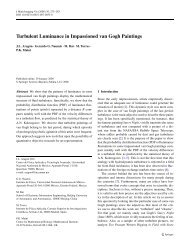
1 Probability density distribution for receiv<strong>in</strong>g an email from Jenny. 41%<br />
of emails is received after five o’clock! . . . . . . . . . . . . . . . . . . . xiv<br />
1.1 Resonant Lewis structures for benzene with s<strong>in</strong>gle and double bonds (left)<br />
and representation of the aromatic structure (right). . . . . . . . . . . . . 7<br />
1.2 Lewis structure of a segment of PPV. . . . . . . . . . . . . . . . . . . . . 8<br />
1.3 Lewis structure of a charged segment of PPV before and after charge mi-<br />
gration. . . . . . . . . . . . . . . . . . . . . . . . . . . . . . . . . . . . 8<br />
1.4 Eigenvalues of equation 1.1 as a function of the reaction coord<strong>in</strong>ate Q. . . 10<br />
1.5 Time evolution for three systems with the same reorganisation energy,<br />
the same angular frequency ω = 5 10 12 s −1 and three different transfer<br />
<strong>in</strong>tegrals J: 1 meV (top), 50 meV (middle) and 300 meV(bottom). . . . . 12<br />
1.6 Time evolution for three systems with the same reorganisation energy, the<br />
same transfer <strong>in</strong>tegral J = 10 meV and three different angular frequencies<br />
ω: 10 12 s −1 (top), 5 10 12 s −1 (middle) and 10 14 s −1 (bottom). . . . . . . . . 14<br />
2.1 Schematic view of a potential energy surface for asymmetric charge trans-<br />
port. λ denotes the reorganisation energy, ∆E the difference <strong>in</strong> energy<br />
between reactants and products <strong>in</strong> their relaxed geometries and ∆Q is the<br />
equilibrium reaction coord<strong>in</strong>ate for the products. . . . . . . . . . . . . . . 20<br />
2.2 Pictorial representation of the vectors discussed <strong>in</strong> deriv<strong>in</strong>g equation 2.26 31<br />
2.3 Pictorial representation of the vectors discussed <strong>in</strong> deriv<strong>in</strong>g equation 2.32 33<br />
iv
2.4 A schematic of one dimensional transport through an energetically and<br />
positionally disordered medium. This figure represents disorder <strong>in</strong> en-<br />
ergy (vertical placement of the transport levels) and <strong>in</strong> transfer <strong>in</strong>tegrals<br />
(thickness of arrows) . . . . . . . . . . . . . . . . . . . . . . . . . . . . 37<br />
2.5 σ versus the value of the dipole moment for five different small conju-<br />
gated molecules (right panel)[44], σd obta<strong>in</strong>ed from equation 2.41 (left<br />
panel) . . . . . . . . . . . . . . . . . . . . . . . . . . . . . . . . . . . . 42<br />
2.6 Pictorial representation of correlation <strong>in</strong> a 100x100x100 cubic lattice of<br />
randomly oriented dipoles. The diameter of the spheres is proportional to<br />
the magnitude of the dipole <strong>in</strong>teraction at that po<strong>in</strong>t, whereas the colour<br />
of the spheres represents the sign of the potential [45] . . . . . . . . . . . 43<br />
2.7 Energy distribution of charges as a function of time after generation [46]. 44<br />
2.8 Schematic of different routes from A to B <strong>in</strong> the direction of the field [46] 45<br />
3.1 A pair of ethylene molecules at a separation of 5 Å . Also shown is the<br />
axis around which one of the two molecules will be rotated to generate<br />
the geometries for which ∆E is calculated. . . . . . . . . . . . . . . . . 62<br />
3.2 Site energy difference for a pair of neutral ethylene molecules as a func-<br />
tion of rotation of one of the molecule about the the C=C bond calcu-<br />
lated by projection of PW91 MOs (circles) and calculated from the differ-<br />
ence <strong>in</strong> quadrupole-monopole <strong>in</strong>teractions calculated classically from the<br />
electrical moments calculated at the PW91 level on an isolated ethylene<br />
molecule (solid l<strong>in</strong>e). . . . . . . . . . . . . . . . . . . . . . . . . . . . . 63<br />
3.3 Site energy difference for a pair of neutral ethylene molecules as a func-<br />
tion of rotation of one of the molecules about the the C=C bond calculated<br />
by projection of PW91 MOs (circles) and calculated from the difference<br />
<strong>in</strong> quadrupole-monopole <strong>in</strong>teractions corrected by the quadrupole <strong>in</strong>duced<br />
dipoles (solid l<strong>in</strong>es). Polarisabilities and electrical moments were calcu-<br />
lated at the PW91 level. . . . . . . . . . . . . . . . . . . . . . . . . . . . 65<br />
v
3.4 Distance dependence of the contribution to ∆E from the <strong>in</strong>duced dipole<br />
<strong>in</strong> a pair of ethylene molecules as a function of separation. The solid<br />
l<strong>in</strong>e corresponds to the contribution from the dipole moment <strong>in</strong>duced by a<br />
quadrupole (i.e. <strong>in</strong> a neutral system), whereas the dotted l<strong>in</strong>e corresponds<br />
to that from the dipole moment <strong>in</strong>duced by a monopole (i.e. <strong>in</strong> a charged<br />
system). . . . . . . . . . . . . . . . . . . . . . . . . . . . . . . . . . . . 67<br />
3.5 Diagram show<strong>in</strong>g the dipoles <strong>in</strong>duced <strong>in</strong> two ethylene molecules oriented<br />
at right angles to each other. (a) Case of po<strong>in</strong>t quadrupoles (neutral cal-<br />
culation). (b) Case of po<strong>in</strong>t charges (charge calculation). For discussion,<br />
please see the text. . . . . . . . . . . . . . . . . . . . . . . . . . . . . . 68<br />
3.6 Dipoles <strong>in</strong>duced on each molecule <strong>in</strong> a pair of neutral ethylene molecules<br />
(upper pannel) and <strong>in</strong> a positively charged pair (lower panel). Notice that,<br />
as shown <strong>in</strong> figure 3.5, <strong>in</strong> a charged system the <strong>in</strong>duced dipoles are larger<br />
than <strong>in</strong> the neutral case, but are <strong>in</strong> opposite directions. . . . . . . . . . . 70<br />
3.7 Two cofacial pentacene molecules and the axis around which one will be<br />
rotated and translated. The <strong>in</strong>set shows the chemical formula of pentacene. 71<br />
3.8 ∆E for pairs of pentacene molecules, calculated us<strong>in</strong>g projection of the<br />
PW91 results (red po<strong>in</strong>ts) and electrostatic results (diamonds). The elec-<br />
trostatic results are calculated us<strong>in</strong>g monopole monopole <strong>in</strong>teractions only<br />
(squares) and us<strong>in</strong>g all <strong>in</strong>teractions up to quadrupole-quadrupole (circles). 72<br />
3.9 Absolute value of the hole transfer <strong>in</strong>tegral as a function of displacement<br />
along the x axis of one of the two pentacene molecules calculated by<br />
projection of ZINDO orbitals (circles) and by the orbital splitt<strong>in</strong>g model<br />
(triangles). The length of the molecule is 14.1 Å . . . . . . . . . . . . . . 74<br />
3.10 HOMO for pentacene calculated at the ZINDO level. . . . . . . . . . . . 74<br />
3.11 Absolute value of the transfer <strong>in</strong>tegral for a pair of pentacene molecules as<br />
a function of rotation around the x axis. The transfer <strong>in</strong>tegral is calculated<br />
by projection of the ZINDO orbitals (circles) and by the orbital splitt<strong>in</strong>g<br />
method (triangles). . . . . . . . . . . . . . . . . . . . . . . . . . . . . . 75<br />
vi
3.12 Absolute value of the transfer <strong>in</strong>tegral for a pair of ethylene molecules<br />
as a function of rotation angle. All curves were obta<strong>in</strong>ed by projective<br />
method applied to PW91 calculations; the different curves are obta<strong>in</strong>ed<br />
by us<strong>in</strong>g different basis sets. . . . . . . . . . . . . . . . . . . . . . . . . 76<br />
3.13 Absolute value of the transfer <strong>in</strong>tegral as a function of displacement along<br />
the x axis of one of the two pentacene molecules. The two curves show<br />
the results from the projective method us<strong>in</strong>g the PW91 functional and<br />
the ZINDO Hamiltonian. The PW91 calculation were performed with a<br />
TVZP basis set. . . . . . . . . . . . . . . . . . . . . . . . . . . . . . . . 77<br />
3.14 Two cofacial HBC molecules and the cartesian axis used <strong>in</strong> the text. The<br />
<strong>in</strong>set shows the chemical formula of HBC. . . . . . . . . . . . . . . . . . 78<br />
3.15 Contour plots of the effective transfer <strong>in</strong>tegral as a function of rotation<br />
about the x and z axis. The molecules are first rotated about the z axis,<br />
then rotated about the x axis <strong>in</strong> such a way as to keep the m<strong>in</strong>imum dis-<br />
tance of approach between the molecules equal to 3.5 Å . . . . . . . . . . 79<br />
3.16 Effective transfer <strong>in</strong>tegral and its components as a function of rotation<br />
about the z axis calculated us<strong>in</strong>g the projective (PRO) and MOO (MOO)<br />
methods. The molecules are at a distance of 3.5 Å . . . . . . . . . . . . . 80<br />
3.17 Countour plots of the dependence on x-y displacement of two molecules<br />
of HBC. The two molecules are at a distance of 3.5 Å. The maximum<br />
radius of the molecule is 6.8 Å. . . . . . . . . . . . . . . . . . . . . . . . 82<br />
4.1 Two monomers of PPV and the scheme of the labels used <strong>in</strong> the rest of the<br />
chapter: ph1...phn will label the phenylene units and vi1...vi2 will label<br />
the v<strong>in</strong>ylene units. The first monomer also has the carbons with bonds to<br />
hydrogen labeled 1 to 6. . . . . . . . . . . . . . . . . . . . . . . . . . . 86<br />
4.2 Experimental and modelled ENDOR spectra of PPV with an applied mag-<br />
netic field parallel and perpendicular to the polymer cha<strong>in</strong> axis. The figure<br />
is from reference [2]. . . . . . . . . . . . . . . . . . . . . . . . . . . . . 87<br />
vii
4.3 Sp<strong>in</strong> density of a polaron on a PPV cha<strong>in</strong> calculated with a PPP Hamil-<br />
tonian. Sites B and C’ correspond to sites 2 and 4 from figure 4.1, sites<br />
B’ and C correspond to sites 1 and 3 from figure 4.1 and sites E and F<br />
correspond to sites 5 and 6 from 4.1. The figure is from reference [2]. . . 88<br />
4.4 Mulliken sp<strong>in</strong> density for different length oligomers of PPV. The x axis<br />
labels position along the cha<strong>in</strong>: the labels ph1, ph2, etc. label the first,<br />
second, etc. phenylene unit of the PPV. Between the phenylene units phn<br />
and phn + 1 lies the v<strong>in</strong>ylene unit v<strong>in</strong>. . . . . . . . . . . . . . . . . . . . 90<br />
4.5 Polaron localisation energy for different length oligomers of PPV calcu-<br />
lated with BHandHLYP. . . . . . . . . . . . . . . . . . . . . . . . . . . 91<br />
4.6 Atomic Mulliken sp<strong>in</strong> density for the a cha<strong>in</strong> of 12 units calculated at the<br />
BHandHLYP (top panel) and AM1 (bottom panel) level. . . . . . . . . . 93<br />
4.7 Mulliken total sp<strong>in</strong> density <strong>in</strong>tegrated on each phenylene and v<strong>in</strong>ylene<br />
unit as a function of cha<strong>in</strong> torsion for an oligomer of length eight. . . . . 94<br />
5.1 The seven unique pairs with greatest hole transfer <strong>in</strong>tegral extracted from<br />
a cluster of twenty molecules of PCBM from its crystal structure grown<br />
<strong>in</strong> chlorobenzene. . . . . . . . . . . . . . . . . . . . . . . . . . . . . . . 100<br />
5.2 Distance dependence of the electron (black circles) and hole (red squares)<br />
transfer <strong>in</strong>tegrals as a function of displacement from the crystal structure<br />
separation. The l<strong>in</strong>es show exponential fits with natural lengths of respec-<br />
tively 0.78 Å and 0.56 Å. . . . . . . . . . . . . . . . . . . . . . . . . . . 102<br />
5.3 Scatter plot of the average sp<strong>in</strong> density for each bonded pair of atoms <strong>in</strong><br />
a cation (circles) or <strong>in</strong> an anion (crosses) versus the percentage change <strong>in</strong><br />
bond length upon charg<strong>in</strong>g. . . . . . . . . . . . . . . . . . . . . . . . . . 104<br />
5.4 Sp<strong>in</strong> density for cation and anion radicals of PCBM. The left panel shows<br />
a front view of the molecules, the right panel a side view. With<strong>in</strong> each<br />
panel the molecule to the left is the anion radical and the molecule to the<br />
right is the cation radical. . . . . . . . . . . . . . . . . . . . . . . . . . . 104<br />
5.5 Zero field mobility for electrons (squares) and holes (circles) <strong>in</strong> PCBM<br />
doped polystyrene as a function of PCBM concentration. . . . . . . . . . 105<br />
viii
5.6 Distance dependance for the transfer <strong>in</strong>tegral for neighbour and nearest<br />
neighbour hopp<strong>in</strong>gs, extracted from the cluster from the crystal structure<br />
of PCBM discussed <strong>in</strong> the text. The transfer <strong>in</strong>tegral is plotted both as a<br />
function of the distance between centres of mass of the PCBM molecules<br />
(above) and as a function of the distance between the centres of the C60<br />
cages (below). This is done because the C60 cages are the electronically<br />
active parts of the molecules. . . . . . . . . . . . . . . . . . . . . . . . 107<br />
5.7 Experimental (full symbols) and modelled (empty symbols) temperature<br />
dependence for prist<strong>in</strong>e MDMO-PPV (triangles) 1:1 MDMO-PPV:PCBM<br />
(circles) and 1:2 MDMO-PPV:PCBM (squares). . . . . . . . . . . . . . . 107<br />
6.1 Chemical formula of the three dialkoxy PPV derivatives studied <strong>in</strong> this<br />
chapter. a) is di-MethoxyPPV(dMeOPPV), b) is di-hexyloxyPPV (dHeOPPV)<br />
and f<strong>in</strong>ally c) is di-decyloxyPPV (dDeOPPV). . . . . . . . . . . . . . . . 113<br />
6.2 Electric field dependence of mobility for dMeOPPV (full squares, pre-<br />
annealed C1 ) for dHeOPPV (empty diamonds, C6) and for dDeOPPV<br />
(empty circles, C10). The figure also shows the electric field dependence<br />
of mobility for dMeOPPV annealed at low temperature (full triangles,<br />
non-annealed C1) and for MDMO-PPV (dotted l<strong>in</strong>e). . . . . . . . . . . . 115<br />
6.3 Representation of the three Euler angles def<strong>in</strong><strong>in</strong>g relative orientation: Φ<br />
and Θ represent the first two Euler rotations about the temporary z and x<br />
axis, Ψ represents the last rotation about the z axis. . . . . . . . . . . . . 117<br />
6.4 Probability distributions of the difference <strong>in</strong> site energies (left panel) and<br />
the logarithm of the transfer <strong>in</strong>tegral (right panel) of two hexamers of<br />
dMeOPPV with a m<strong>in</strong>imum separation of 3.5 Å . Probability distributions<br />
(vertical bars) are compared to a normal distribution (solid l<strong>in</strong>e). . . . . . 120<br />
6.5 Distance dependence of the standard deviation <strong>in</strong> values of ∆E. . . . . . 121<br />
6.6 Scatter plot of the absolute value of ∆E aga<strong>in</strong>st the logarithm of the trans-<br />
fer <strong>in</strong>tegral log(J) (a). Also shown is the scatter plot of log(J) versus the<br />
centre to centre separation d (b) and the scatter plot of ∆E versus d (c). . . 122<br />
ix
6.7 The three spiro-l<strong>in</strong>ked tryarilam<strong>in</strong>e derivatives considered <strong>in</strong> this study.<br />
From left to right they are 2,2’,7,7’-tetrakis-(N,N-diphenylhenylam<strong>in</strong>o)-<br />
9,9’-spirobifluorene (spiro-unsub), 2,2’,7,7’-tetrakis-(N,N-di-m-methylphenylam<strong>in</strong>o)-<br />
9,9’-spirobifluorene (spiro-Me) and f<strong>in</strong>ally 2,2’,7,7’-tetrakis-(N,N-di-4-<br />
methoxyphenylam<strong>in</strong>o)-9,9’-spirobifluorene (spiro-MeO) . . . . . . . . . . 123<br />
6.8 Histogram of ∆E for spiro-unsub (dashed l<strong>in</strong>e), spiro-Me (dotted l<strong>in</strong>e)<br />
and spiro-MeO (full l<strong>in</strong>e). The standard deviation for the three materials<br />
is 8 meV for spiro-unsub, 10 meV for spiro-Me and 15 meV spiro-MeO. . 125<br />
7.1 Schematic representation of the morphology model used by Dr. S. Athanosopou-<br />
los to describe PFO and def<strong>in</strong>itions of the parameters govern<strong>in</strong>g the rel-<br />
ative position and orientation of molecules. (a) The polymer cha<strong>in</strong>s are<br />
packed hexagonally, with the cha<strong>in</strong> axis perpendicular to the electric field.<br />
(b) Each trimer is allowed to rotate by a torsion φ and can be displaced<br />
by a distace ∆r <strong>in</strong> the direction perpendicular to the cha<strong>in</strong> axis and can<br />
slip by a distance dz parallell to the cha<strong>in</strong> axis. (c) Top view of the central<br />
planes of two trimers, show<strong>in</strong>g the torsion angles φ1 and φ2 (∆φ = φ2−φ1)<br />
and the polar angle α. . . . . . . . . . . . . . . . . . . . . . . . . . . . . 131<br />
7.2 HOMO (left) and HOMO-1 (right), of the restricted open shell orbitals of<br />
a fluorene trimer with one of the hydrogen end groups miss<strong>in</strong>g. . . . . . . 132<br />
7.3 Contour plot of log(|J| 2 ) as a function of relative torsion angle dφ and the<br />
polar angle α which describes position. Notice how the values of these<br />
<strong>in</strong>tercha<strong>in</strong> transfer <strong>in</strong>tegrals are always much smaller than the <strong>in</strong>tracha<strong>in</strong><br />
transfer <strong>in</strong>tegrals from figure 7.5. . . . . . . . . . . . . . . . . . . . . . 135<br />
7.4 Distance dependence of the transfer <strong>in</strong>tegral squared on distance for φ =<br />
150 ◦ and α = 0 ◦ (squares) and for φ = 0 ◦ and α = 0 ◦ (circles). . . . . . . 135<br />
7.5 Intracha<strong>in</strong> transfer <strong>in</strong>tegrals squared as a function of relative torsion φ for<br />
two trimers. . . . . . . . . . . . . . . . . . . . . . . . . . . . . . . . . . 136<br />
x
7.6 Difference between forward and backward rates for an ordered lattice<br />
as a function the torsion angle φ at which the trimers are set. √ F =<br />
200(V/cm) 1/2 (solid l<strong>in</strong>e), 400(V/cm) 1/2 (dotted l<strong>in</strong>e), 600(V/cm) 1/2 (dashed<br />
l<strong>in</strong>e), 800(V/cm) 1/2 (cha<strong>in</strong>ed l<strong>in</strong>e, one dot), 1000(V/cm) 1/2 (cha<strong>in</strong>ed l<strong>in</strong>e,<br />
two dots). . . . . . . . . . . . . . . . . . . . . . . . . . . . . . . . . . . 137<br />
7.7 Dependence of mobility on the square root of the applied electric field<br />
for: the ordered morphology with φ = 0 ◦ (open triangles), the ordered<br />
morphology with φ = 20 ◦ (diamonds), the morphology with disordered<br />
torsions (full squares), the optimally disordered morphology (full trian-<br />
gles) and the experimental data on alligned PFO from reference [3] (full<br />
circles).The optimally ordered morphology corresponds to when neigh-<br />
bours <strong>in</strong> the direction of the field have a relative torsion φ of 150 ◦ . The<br />
lattice constant for the hexagonal lattice is 6.5 Å . . . . . . . . . . . . . . 138<br />
7.8 Chemical structure of the various derivatives of HBC considered <strong>in</strong> this<br />
study . . . . . . . . . . . . . . . . . . . . . . . . . . . . . . . . . . . . . 142<br />
7.9 ToF results for several selected snapshots, together with the averaged over<br />
the MD run displacement current (left). Block averages over 10, 20, ...<br />
190 snapshots. (right) . . . . . . . . . . . . . . . . . . . . . . . . . . . 144<br />
7.10 Displacement current for different numbers of molecules <strong>in</strong> a column.<br />
Average over 200 snapshots at an electric field of 10 5 Vcm −1 . . . . . . . . 145<br />
7.11 Radial distribution function along the z direction for all six derivatives<br />
considered <strong>in</strong> this study. . . . . . . . . . . . . . . . . . . . . . . . . . . . 145<br />
7.12 Distribution <strong>in</strong> logarithm of the effective transfer <strong>in</strong>tegrals for holes squared<br />
for 20 columns of 100 molecules each. . . . . . . . . . . . . . . . . . . . 148<br />
xi
List of Tables<br />
5.1 Table of the transfer <strong>in</strong>tegral for holes Jh and for electrons Je. n is the<br />
number of such pairs <strong>in</strong> a cluster of 20 molecules. dcoc is the separation<br />
between the centres of the fullerene cages for the pair of molecules. The<br />
labels a-g label the pairs accord<strong>in</strong>g to figure 5.1 . . . . . . . . . . . . . . 100<br />
5.2 Reorganisation energies for anion. . . . . . . . . . . . . . . . . . . . . . 102<br />
5.3 Reorganisation energies for cation. . . . . . . . . . . . . . . . . . . . . . 102<br />
6.1 GDM parameters for the various dialkoxy PPV derivatives. . . . . . . . . 115<br />
6.2 GDM energetic disorder σGDM and standard deviation <strong>in</strong> distribution of<br />
site energy difference calculated us<strong>in</strong>g distributed Multipole analysis (<br />
σDMA ) . . . . . . . . . . . . . . . . . . . . . . . . . . . . . . . . . . . 125<br />
7.1 Electron (e) and hole (h) mobilities (cm 2 V −1 s −1 ) of different compounds<br />
calculated us<strong>in</strong>g time-of-flight (ToF) and master equation (ME) methods,<br />
<strong>in</strong> comparison with experimentally measured PR-TRMC mobilities. Also<br />
shown are the nematic order parameter Q and the average vertical separa-<br />
tion between cores of HBC molecules h (Å). . . . . . . . . . . . . . . . . 147<br />
xii
Acknowledgments<br />
I would like to acknowledge all the help and support from my colleagues at Imperial<br />
College and my collaborators. None of my work would have been possible without my<br />
supervisor, Jenny Nelson, who provided guidance and advice whilst allow<strong>in</strong>g me absolute<br />
freedom. On no scientific topic was she unable of either provid<strong>in</strong>g expertise or po<strong>in</strong>t<strong>in</strong>g<br />
me <strong>in</strong> the correct direction. Her stakhanovist attitude to work is <strong>in</strong>spirational and is best<br />
exemplified by the probability distribution for receiv<strong>in</strong>g emails from her (shown <strong>in</strong> figure<br />
1).<br />
I received a lot of editorial help <strong>in</strong> the writ<strong>in</strong>g of the thesis: from my father, Rysia,<br />
most of the people I shared an office with <strong>in</strong> room H724 (especially Graeme) and ob-<br />
viously from Jenny! Rysia’s help <strong>in</strong> proof-read<strong>in</strong>g at the 11th hour was <strong>in</strong>dispensable.<br />
Kristian Sylvester-Hvid also provided useful <strong>in</strong>sight <strong>in</strong> the <strong>in</strong>troduction of the thesis.<br />
Thanks to Bhavna and Carolyn for their efficient runn<strong>in</strong>g of the group.<br />
I would like to thank, or rather apologise to, those who I have pestered with program-<br />
m<strong>in</strong>g issues, especially my housemates Pete and Joe.<br />
I would also like to thank those who helped straighten out a few of the bugs <strong>in</strong> my<br />
code: Joe Kwiatkowski, Stavros Athanasopoulos from Bath University and David Reha<br />
from Leeds University.<br />
A word of thanks should go to Ian Gould and Emilio Palomares for help<strong>in</strong>g me nav-<br />
igate my first steps <strong>in</strong> Quantum Chemistry. The staff at the EPSRC centre for computa-<br />
tional chemistry are also thanked for all the assistance <strong>in</strong> learn<strong>in</strong>g to use computational<br />
packages and computer time.<br />
Many of the <strong>in</strong>vestigations <strong>in</strong> this thesis were collaborative and I want to especially<br />
acknowledge the experimental efforts of Sachetan Tuladhar, whose results are discussed<br />
<strong>in</strong> chapter five and six . A special word of thank should go to Sachetan for be<strong>in</strong>g such a<br />
xiii
Probability Density<br />
0.1<br />
0.05<br />
0<br />
0 4 8 12 16 20<br />
Arrival Time (hr)<br />
Figure 1: Probability density distribution for receiv<strong>in</strong>g an email from Jenny. 41% of<br />
emails is received after five o’clock!<br />
pleasant room mate <strong>in</strong> the undercroft. The time of flight code I used has been developed by<br />
many: Jenny Nelson, Amanda Chatten, Rosemary Chandler and Joe Kwiatkowski. The<br />
work on hexabenzorononene is the fruit of a fruitful collaboration with Denis Andrienko,<br />
who was also a most courteous host <strong>in</strong> Ma<strong>in</strong>z. For the work on poly(dioctylfluorene) I<br />
would like to thank the group at Bath University, especially Pete Watk<strong>in</strong>s who did much<br />
of the work on develop<strong>in</strong>g their Monte Carlo code and morphology model.<br />
A word of thanks goes also to the research groups which I have been priviledged to<br />
visit and the staff who took care of me: Jérôme Cornil and Davide Beljonne from the Uni-<br />
versity of Mons-Ha<strong>in</strong>aut, Jean-Luc Brédas and Demetrio da Silvha Filho from Georgia<br />
Institute of technology and f<strong>in</strong>ally Kristian Sylvester-Hvid for host<strong>in</strong>g me <strong>in</strong> Copenhagen.<br />
F<strong>in</strong>ally I would like to thank all the rest of the people <strong>in</strong> the physics deparment who<br />
have provided lunch brakes and coffee break discussions: Graeme, the two Matts, Rob,<br />
Peter, Thil<strong>in</strong>i, Jessica, Joe, Jarvist, Dan, Rahul, Dave Johnson, Markus, Marianne, Ben,<br />
Just<strong>in</strong>, Tom, Mariano, Jony, Ben. Paul Stavr<strong>in</strong>ou also deserved mention for <strong>in</strong>terest<strong>in</strong>g<br />
discussion.<br />
xiv
Mike Bearpark and Martial Boggio-Pasqua have guided me through my PhD on CASSCF<br />
calculations. The results are not <strong>in</strong> this thesis, but I am greatly <strong>in</strong>debted to them for the<br />
<strong>in</strong>terest<strong>in</strong>g tutor<strong>in</strong>g they gave me.<br />
The last word of thanks is to the reader: I hope you do not f<strong>in</strong>d this too bor<strong>in</strong>g!<br />
xv
Abstract<br />
In this thesis we discuss the calculation of charge transport parameters <strong>in</strong> conjugated<br />
solids. We aim to elucidate the role of chemical structure and molecular pack<strong>in</strong>g <strong>in</strong> de-<br />
term<strong>in</strong><strong>in</strong>g charge transport characteristics. In chapter two we discuss the rate equation<br />
from Marcus theory used throughout the thesis and its parameters: electronic coupl<strong>in</strong>g,<br />
reorganisation energy and site energy difference. We also discuss the Gaussian Disor-<br />
der Model as an example of a lattice based simulation of charge transport. We show that<br />
lattice simulations are limited because of the difficulty <strong>in</strong> relat<strong>in</strong>g model parameters to mi-<br />
croscopic properties of a material. In chapter three we present fast methods of calculat<strong>in</strong>g<br />
transfer <strong>in</strong>tegrals and site energies for pairs of molecules. We will use these methods <strong>in</strong><br />
chapters six and seven, <strong>in</strong> which calculations on large numbers of pairs of molecules are<br />
carried out. These fast but approximate methods are shown to be <strong>in</strong> agreement with more<br />
ab-<strong>in</strong>itio methods. In chapter four we discuss localisation of charges along the backbone<br />
of conjugated polymers and argue that thermal fluctuations are of greater importance than<br />
polaron b<strong>in</strong>d<strong>in</strong>g energies <strong>in</strong> affect<strong>in</strong>g localisation. In chapter five we calculate transfer<br />
<strong>in</strong>tegrals and reorganisation energies for electrons and holes <strong>in</strong> a fullerene derivative <strong>in</strong><br />
order to justify the choice of parameters <strong>in</strong> a lattice based simulation. In chapter six we<br />
use the fast methods for calculat<strong>in</strong>g transfer <strong>in</strong>tegrals and site energies to rationalise the<br />
Gaussian Disorder Model parameters of two families of materials: dialkoxy polypara-<br />
phenylenev<strong>in</strong>ylenes and triarylam<strong>in</strong>e derivatives. The differences <strong>in</strong> energetic disoder<br />
between the materials is attributed to electrostatic effects. In chapter seven we calcu-<br />
late charge transport parameters for simulated morphologies of the crystall<strong>in</strong>e phase of<br />
poly(dioctylfluorene) and of the discotic liquid crystal mesophase of different hexabenzo-<br />
coronene derivatives. In the case of poly(dioctylfluorene) calculations of mobility help to<br />
shed light on molecular pack<strong>in</strong>g. In the case of hexabenzocoronene the availability of a<br />
good morphology model leads, with no free parameters, to values of mobility <strong>in</strong> excellent<br />
agreement with experimental data.
List of Symbols and Abbreviations<br />
J: Electronic overlap<br />
MOO: Molecular Orbital Overlap: a method to calculate J based on a simplification of<br />
ZINDO<br />
INDO: Intermediate Neglect of Differential Overlap method<br />
ZINDO: Zerner’s Intermediate Neglect of Differential Overlap method [1]<br />
∆E: Site energy difference<br />
λ: Reorganisation energy<br />
S CF: Self Consistent Field: a method to determ<strong>in</strong>e the electronic energy of a system<br />
where the Fock matrix is dependent on the wavefunction; the procedure is therefore re-<br />
peated until the wavefunction obta<strong>in</strong>ed by diagonalis<strong>in</strong>g the Fock matrix and the Fock<br />
matrix obta<strong>in</strong>ed from the wavefunction are consistent with each other<br />
HOMO: Highest Occupied Molecular Orbital<br />
LUMO: Lowest Unoccupied Molecular Orbital<br />
µ ν: Labels for molecular (or atomic) orbitals; µ is also the mobility.<br />
A B: Labels for molecules<br />
i j: Labels for electrons<br />
a b: Labels for atoms<br />
x y z α β: Labels for x,y and z coord<strong>in</strong>ates or for generic coord<strong>in</strong>ate labels (α β)<br />
Ψ: Electron wavefunction<br />
χ: Nuclear wavefunction<br />
Ψ: Slater determ<strong>in</strong>ant: a comb<strong>in</strong>ation of molecular orbitals which ensures the anti-symmetric<br />
nature of the wavefunction<br />
ψ: Molecular orbital<br />
φ: Atomic orbital<br />
S : Overlap matrix<br />
P: The density matrix P = � µ occupied φ t µφµ<br />
Q: Quadrupole moment<br />
P: Polarisability<br />
a0: Bohr radius<br />
1
e: Magnitude of the charge of an electron<br />
k: Boltzmann’s constant<br />
T: Temperature<br />
DMA: Distributed Multipole Analysis<br />
U: An electrostatic <strong>in</strong>teraction<br />
σ: Energetic disorder or a bond formed by sp hybridised orbitals or σ overlap (i.e. the<br />
overlap between p atomic orbitals symmetric about the vector jo<strong>in</strong><strong>in</strong><strong>in</strong>g the two atomic<br />
centres)<br />
π: Bonds formed by p orbitals or π overlap (i.e. the overlap between p atomic orbitals<br />
antisymmetric about the vector jo<strong>in</strong><strong>in</strong><strong>in</strong>g the two atomic centres)<br />
C: Matrix represent<strong>in</strong>g all the molecular orbitals <strong>in</strong> a basis set; each row corresponds to a<br />
molecular orbital<br />
Q: Nuclear coord<strong>in</strong>ates<br />
q: Electronic coord<strong>in</strong>ates<br />
ω: Angular frequency<br />
F: Electric field<br />
2
Bibliography<br />
[1] J. Ridley and M. Zerner, An Intermediate Neglect of Differential Overlap Technique<br />
for Spectroscopy: Pyrrole and the Az<strong>in</strong>es, Theoretica Chimica Acta, 32, 111 (1973)<br />
3
Chapter 1<br />
Introduction<br />
1.1 Why is a Theoretical Study of <strong>Charge</strong> <strong>Transport</strong> Nec-<br />
essary to the Design of Better Devices?<br />
Ever s<strong>in</strong>ce the discovery of conductivity <strong>in</strong> trans-polyacetylene [1], study of the electronic<br />
properties of organic molecules has been very <strong>in</strong>tense. The field was further stimulated<br />
by the discovery of light emitt<strong>in</strong>g polymers [2] and of photo<strong>in</strong>duced charge separation<br />
<strong>in</strong> polymer fullerene blends [3], which stimulated the development of, respectively, light<br />
emitt<strong>in</strong>g diodes and solar cells. The reason for these high levels of <strong>in</strong>terest is that if it were<br />
possible to design materials with the opto-electronic properties of <strong>in</strong>organic semiconduc-<br />
tors and the mechanical and process<strong>in</strong>g properties of plastics, the applications would be<br />
revolutionary. Solution processability would allow fabrication of devices <strong>in</strong> cont<strong>in</strong>uous<br />
<strong>in</strong>dustrial processes [4, 5], thus reduc<strong>in</strong>g costs. Plastics are also flexible and light-weight<br />
compared to rigid, brittle <strong>in</strong>organic semiconductors: this could open the door to <strong>in</strong>tegra-<br />
tion of electronic devices on different subtrates. It seems to us that the area which will<br />
show the greatest long term benefits is organic photovoltaics (PV): <strong>in</strong>organic PV is lim-<br />
ited <strong>in</strong> applicability by its high cost, both due to material costs (solar cells are large area<br />
devices) and process<strong>in</strong>g costs (fabricat<strong>in</strong>g a PV module is a complex process). For both<br />
these reasons, the potential low cost and ease of process<strong>in</strong>g of organic materials would<br />
have a great impact.<br />
Many different designs of solar cells based on organic materials have been proposed,<br />
4
for example: dye sensitised solar cells [6], bulk heterojunction cells [7, 8], composite<br />
cadmium selenide/polymer solar cells [9], cells based on self organised liquid crystals<br />
[11]. In all these systems three processes must occur <strong>in</strong> order for a photocurrent to be<br />
collected at the electrodes: photons must be absorbed, charges must be separated and fi-<br />
nally charges must be able to migrate to the electrodes. <strong>Charge</strong> mobility is important both<br />
because it sets the maximum space charge limited current obta<strong>in</strong>able by the device [12]<br />
and because, if transport is slower than charge absorption or charge separation, it causes<br />
bottlenecks and <strong>in</strong>creased recomb<strong>in</strong>ation [13]. In this thesis, we study the parameters con-<br />
troll<strong>in</strong>g charge dynamics <strong>in</strong> organic materials. In particular we will argue for the need of<br />
electronic structure calculations to elucidate the relationship between chemical structure<br />
and charge transport characteristics. We want to suggest that our understand<strong>in</strong>g of the<br />
fundamental mechanism beh<strong>in</strong>d charge transport and the speed of computers is now suf-<br />
ficient to allow an understand<strong>in</strong>g of charge mobility based on the fundamental electronic<br />
properties of molecules and that this is the only path which will allow disentanglement<br />
of the various chemical and physical causes for device performance, therefore allow<strong>in</strong>g<br />
better material and device design.<br />
The thesis is organised as follows: <strong>in</strong> chapter two we describe the non-adiabatic, Mar-<br />
cus high temperature charge transfer equation and methods from the literature to calculate<br />
its parameters; we also discuss some lattice based models of charge mobility. In chapter<br />
three we discuss fast methods of calculat<strong>in</strong>g the parameters of the Marcus charge transfer<br />
equation. In chapter four we discuss the nature of charged radicals on polymer cha<strong>in</strong>s.<br />
The rest of the thesis is dedicated to apply<strong>in</strong>g the methods developed to expla<strong>in</strong><strong>in</strong>g ex-<br />
perimental charge transport characteristics of conjugated materials. In chapter five we<br />
exam<strong>in</strong>e the dependence on fullerene concentration of electron and hole mobilities <strong>in</strong><br />
blends of fullerene and conjugated polymer. In chapter six we calculate charge transport<br />
parameters <strong>in</strong> pairs of molecules <strong>in</strong> random orientations and compare these results to pa-<br />
rameters from lattice models of mobility. In chapter seven we run full-blown simulations<br />
of molecular morphology and electronic properties for polymers and discotic liquid crys-<br />
tals <strong>in</strong> an effort to reproduce charge transport characteristics with a m<strong>in</strong>imal number of<br />
adjustable parameters. F<strong>in</strong>ally we will give a brief of conclusion of the thesis. The rest of<br />
5
this chapter <strong>in</strong>troduces some concepts about charge transfer <strong>in</strong> conjugated materials.<br />
1.2 Conjugated Materials<br />
The properties of conjugated materials are based on the nature of covalent bonds between<br />
carbon, nitrogen, sulfur and oxygen. Specifically, they are based on the properties of sp 2<br />
bonds <strong>in</strong> carbon atoms. In order to better understand the different types of bond<strong>in</strong>g that<br />
carbon is capable of let us consider three compounds: ethane (C2H6), ethene (C2H4) and<br />
ethyne (C2H2). In these three compounds, each carbon forms bonds with either four, three<br />
or two other atoms. These three different behaviours depend on how the 2s and 2p atomic<br />
orbitals on carbon hybridise to form bonds: <strong>in</strong> ethane four σ bonds are formed by mix<strong>in</strong>g<br />
a s<strong>in</strong>gle 2s orbital with three 2p orbitals. These σ orbitals are therefore known as sp 3<br />
orbitals. In ethene only three σ bonds are formed by mix<strong>in</strong>g a 2s orbital with two 2p<br />
orbitals. This is sp 2 hybridazation. In ethyne, a s<strong>in</strong>gle σ bond is formed by mix<strong>in</strong>g a 2s<br />
and a 2p orbital. This is sp 1 hybridazation. These three types of orbitals are responsible<br />
for the formation of the bonds which determ<strong>in</strong>e the fundamental geometrical features of<br />
the three molecules. Us<strong>in</strong>g the pr<strong>in</strong>ciple that orbitals will tend to repel each other we can<br />
predict the bond angles <strong>in</strong> the three materials: <strong>in</strong> ethane the bonds around each carbon<br />
are <strong>in</strong> a tetrahedral arrangement, <strong>in</strong> ethene they are triangular and <strong>in</strong> ethyne the bonds are<br />
l<strong>in</strong>ear. In the case of sp 2 and sp 1 hybridasation, one and two 2p orbitals respectively are<br />
left un-hybridised: these orbitals participate <strong>in</strong> bond<strong>in</strong>g by form<strong>in</strong>g a double and a triple<br />
bond respectively between the carbons. A conjugated material is one <strong>in</strong> which all bonds<br />
are either sp 2 or sp 1 hybridised, result<strong>in</strong>g <strong>in</strong> an alternation of s<strong>in</strong>gle and double bonds. As<br />
shown <strong>in</strong> figure 1.1, <strong>in</strong> compounds such as benzene different ways of alternat<strong>in</strong>g s<strong>in</strong>gle<br />
and double bonds leads to different structures with the same energy: these structures<br />
can mix together form<strong>in</strong>g lower energy structures where <strong>in</strong>stead of alternat<strong>in</strong>g s<strong>in</strong>gle and<br />
double bonds, there are only aromatic bonds. These resonances are responsible for the<br />
high stability of aromatic compounds.<br />
σ and π bonds are so called because they are either symmetric or antisymmetric with<br />
respect to the axis connect<strong>in</strong>g the two atoms participat<strong>in</strong>g <strong>in</strong> bond<strong>in</strong>g. This expla<strong>in</strong>s<br />
why σ bonds are strong and participate more <strong>in</strong> determ<strong>in</strong><strong>in</strong>g the geometrical structure<br />
6
Figure 1.1: Resonant Lewis structures for benzene with s<strong>in</strong>gle and double bonds (left) and<br />
representation of the aromatic structure (right).<br />
of molecules: σ orbitals are symmetric across the b<strong>in</strong>d<strong>in</strong>g direction and therefore have<br />
large overlap <strong>in</strong>tegrals, π orbitals, conversely, rely on overlap of the lobes of parallel 2p<br />
orbitals and are much weaker. This observation, that 2p orbitals must be parallel to form<br />
bonds, leads us to understand why ethene is planar: if the two triangles formed by each<br />
carbon and the two hydrogens bonded to them are not parallel, the 2p bonds on each atom<br />
are not capable of form<strong>in</strong>g a bond. So sp 2 hybridisation implies the formation of planar<br />
structures, with double bonds formed by the rema<strong>in</strong>g 2p orbitals.<br />
The <strong>in</strong>terest<strong>in</strong>g electronic properties of conjugated materials is delocalisation. Often<br />
the concept of delocalisation is expla<strong>in</strong>ed by argu<strong>in</strong>g that when the unhybridised p atomic<br />
orbitals on each atom <strong>in</strong>teract to form molecular π orbitals, these π orbitals are delocalised<br />
over the whole molecule. This is certa<strong>in</strong>ly true, however it is not a property unique to π<br />
orbitals, also the hybridised sp 2 atomic orbitals <strong>in</strong>teract to form delocalised σ orbitals. In<br />
my op<strong>in</strong>ion what is special about p conjugated systems is that charged or neutral excita-<br />
tions are delocalised, <strong>in</strong> the sense that they can migrate along the molecule with relatively<br />
small amounts of energy. As an example of this take polyparaphenylenev<strong>in</strong>ylene (PPV).<br />
This p conjugated polymer is shown <strong>in</strong> figure 1.2. If it becomes charged, its Lewis struc-<br />
ture is similar to figure 1.3; <strong>in</strong> this figure the dot represents an unpaired electron and the<br />
7
Figure 1.2: Lewis structure of a segment of PPV.<br />
Figure 1.3: Lewis structure of a charged segment of PPV before and after charge migration.<br />
”+” represents a charge. What we mean to represent <strong>in</strong> this figure is that, upon charg<strong>in</strong>g,<br />
the bond order<strong>in</strong>g changes mak<strong>in</strong>g the structure less aromatic and more qu<strong>in</strong>oid. This<br />
localised qu<strong>in</strong>oid deformation can easily travel along the cha<strong>in</strong> as it only <strong>in</strong>volves the<br />
break<strong>in</strong>g and reform<strong>in</strong>g of loosely bound bonds. This therefore seems to us to be the<br />
fundamental property of conjugated systems: the nature of π bonds is such that they can<br />
be easily broken and reformed without the significant rearrangement of bonds that would<br />
occur if σ bonds were broken.<br />
1.3 <strong>Charge</strong> <strong>Transport</strong> <strong>in</strong> Conjugated Materials<br />
In chapter two we will provide a formal description of non-adiabatic charge transfer, but <strong>in</strong><br />
this section we briefly describe three possible regimes for charge transfer <strong>in</strong> a conjugated<br />
8
material: delocalisation, adiabatic transfer and non-adiabatic transfer. S<strong>in</strong>ce most of our<br />
efforts are computational, rather than provid<strong>in</strong>g a review of analytical charge transfer<br />
models such as can be found <strong>in</strong> references [14, 15], we will implement a simple quantum<br />
dynamical simulation from a simple semi-classical Hamiltonian. In this section we mean<br />
to simply exemplify different possible regimes of charge transfer.<br />
We write a Hamiltonian for charge transfer with two non-<strong>in</strong>teract<strong>in</strong>g (diabatic) states<br />
whose energies depend quadratically on a s<strong>in</strong>gle reaction coord<strong>in</strong>ate Q. Electron-phonon<br />
coupl<strong>in</strong>g is <strong>in</strong>troduced by displac<strong>in</strong>g the potential energy parabula by a distance Q0. At<br />
the nuclear coord<strong>in</strong>ate where the energy of state |0 > is m<strong>in</strong>imised the potential energy for<br />
state |1 > is ω2 Q0 2<br />
2 . This quantity is called the reorganisation energy and is an expression of<br />
electron-phonon coupl<strong>in</strong>g. In the case of the polymers depicted <strong>in</strong> figure 1.3, the reaction<br />
coord<strong>in</strong>ate Q could represent go<strong>in</strong>g from an aromatic to a qu<strong>in</strong>oid structure. Electronic<br />
coupl<strong>in</strong>g between the two diabatic states is described by a transfer <strong>in</strong>tegral J. In state<br />
representation, us<strong>in</strong>g mass weighted coord<strong>in</strong>ates, the Hamiltonian for the system is:<br />
ˆHe = ω2 Q 2<br />
2 |0 >< 0| + ω2 (Q − Q0) 2<br />
2<br />
|1 >< 1| + (J|0 >< 1| + J ∗ |1 >< 0|) (1.1)<br />
Figure 1.4 shows the eigenvalues of this Hamiltonian represented as a function of the<br />
reaction coord<strong>in</strong>ate Q for typical values of ω and Q0.<br />
If the electronic coupl<strong>in</strong>g is of the same order of magnitude as ω2 Q0 2<br />
2 , the system is <strong>in</strong><br />
the delocalised regime. In order to dist<strong>in</strong>guish the other two regimes, we have to consider<br />
the relative time scales for nuclear and electronic transitions. Nuclear oscillations occur<br />
on a timescale of ω −1 ; electronic transitions between the diabatic states, conversely, occur<br />
on a time scale of �/J. If the timescale for electronic transitions is much faster than<br />
that for nuclear motion, i.e. if J is large compared to �ω, charge transfer will occur<br />
gradually as the system oscillates along the potential for the adiabatic states (that is for<br />
the eigenfunction of the Hamiltonian shown <strong>in</strong> equation 1.1 ). If J is small compared to<br />
�ω, the electronic states do not have the time to rearrange themselves as the nuclei vibrate<br />
and the system oscillates along one of the diabatic potential energy surfaces. Each time<br />
the potential energies for each diabatic state are resonant, i.e. when Q = Q0/2 is reached,<br />
the transfer <strong>in</strong>tegral J will set a f<strong>in</strong>ite probability for cross<strong>in</strong>g from one diabatic state to<br />
9
Energy / eV<br />
1<br />
0.5<br />
0<br />
-1 0 1 2<br />
Nuclear coord<strong>in</strong>ates Q / Q<br />
0<br />
Figure 1.4: Eigenvalues of equation 1.1 as a function of the reaction coord<strong>in</strong>ate Q.<br />
another.<br />
In order to perform a simulation of the dynamics of the evolution of the system, we<br />
will use the Ehrenfest approximation. In other words, we assume that the nuclear motion<br />
can be treated classically and that the force on the nuclei is simply the expectation value<br />
of the force operator ˆF = − ˆ He . The set of coupled differential equations we solve is:<br />
Q<br />
˙Pe = i<br />
� [ ˆHe, Pe] (1.2a)<br />
�<br />
F = Tr − d ˆHe<br />
dQ Pe<br />
�<br />
(1.2b)<br />
¨Q = F (1.2c)<br />
where Pe is the density matrix for the electronic system, the square brackets denote tak-<br />
<strong>in</strong>g the commutator and Tr{.} denotes tak<strong>in</strong>g the trace. We numerically <strong>in</strong>tegrate these<br />
equations of motion us<strong>in</strong>g the GNU octave program. In all simulations we scale the mass<br />
weighted length scale so that ω2 Q0 2<br />
2<br />
= 0.3eV. In all cases we start the simulation with a<br />
large potential energy correspond<strong>in</strong>g to a displacement of −Q0 to ensure that the system<br />
10
has sufficient energy to reach the cross<strong>in</strong>g po<strong>in</strong>t of the two diabatic surfaces. We also pre-<br />
pare the electronic system so that at time zero it is <strong>in</strong> the diabatic state |0 >, i.e. take the<br />
<strong>in</strong>itial condition Pe(t = 0) = |0 >< 0|. We then make two comparisons. First we keep the<br />
angular frequency fixed at ω = 5 10 12 s −1 and <strong>in</strong>crease the transfer <strong>in</strong>tegral from 1 meV to<br />
500 meV to illustrate the transition of charge transfer characteristics from non-adiabatic to<br />
adiabatic and f<strong>in</strong>ally to delocalised charge transfer. In the second comparison we keep the<br />
transfer <strong>in</strong>tegral fixed at 10 meV and vary ω from 10 12 s −1 to 10 14 s −1 to demonstrate that<br />
adiabaticity does not result so much from the relative values of J and the reorganisation<br />
energy, but more from the relative values of ω and J/�. In order to exemplify the time<br />
evolution of the system we look at two quantities: the nuclear coord<strong>in</strong>ate Q and Ple f t, the<br />
expectation value of f<strong>in</strong>d<strong>in</strong>g the system <strong>in</strong> diabatic state |0 >. Ple f t is calculated by tak<strong>in</strong>g<br />
the follow<strong>in</strong>g trace over the density matrix: Tr {|0 >< 0|Pe}. We would like to strongly<br />
stress that this simulation has only the purpose of illustrat<strong>in</strong>g graphically different transfer<br />
regimes and that it ignores issues crucial to determ<strong>in</strong><strong>in</strong>g charge transfer rates, such as the<br />
role of nuclear wavefunction overlap, the appropriateness of apply<strong>in</strong>g Ehrnfest dynamics<br />
to non-adiabatic problems and the role of decoherence.<br />
Figure 1.5 shows the time evolution for systems with the same angular frequency and<br />
different transfer <strong>in</strong>tegrals. The top panel shows an example of non-adiabatic transfer,<br />
with the timescale for transition between diabatic states beg<strong>in</strong> �/J = 6.6 10 −13 s and with<br />
the time scale for nuclear motion be<strong>in</strong>g 1/ω = 2.0 10 −13 s. The nuclear system is oscillat-<br />
<strong>in</strong>g along the diabatic surface and <strong>in</strong> fact the midpo<strong>in</strong>t for oscillation is 0, the position of<br />
the bottom of the left parabula. Each time the nuclear coord<strong>in</strong>ate passes through Q0<br />
2 , Ple f t<br />
jumps abruptly and there is a f<strong>in</strong>ite probability of f<strong>in</strong>d<strong>in</strong>g the system <strong>in</strong> the diabatic state<br />
|1 >.<br />
The middle panel of figure 1.5 shows time evolution for the same ω but for a dif-<br />
ferent value of J of 50 meV. In this case the timescale for diabatic transitions is �/J =<br />
1.3 10 −14 s: electronic transitions occur faster than the nuclear motion. In fact each time<br />
that the system goes through Q0<br />
2 , Ple f t switches from left to right, show<strong>in</strong>g that electronic<br />
transitions take place fully and not partially as <strong>in</strong> the non-adiabatic regime. Look<strong>in</strong>g at<br />
the nuclear displacement, we notice that the midpo<strong>in</strong>t of the oscillation occurs at Q0 , not 2<br />
11
Displacement / Q 0<br />
Displacement / Q 0<br />
Displacement / Q 0<br />
1.5<br />
1<br />
0.5<br />
0<br />
-0.5<br />
-1<br />
1.6<br />
1.4<br />
1.2<br />
1<br />
0.8<br />
0.6<br />
0.4<br />
0.2<br />
0<br />
-0.2<br />
-0.4<br />
-0.6<br />
2<br />
1.5<br />
1<br />
0.5<br />
0<br />
-0.5<br />
-1<br />
0 1e-12 2e-12 3e-12 4e-12 5e-12 6e-12 7e-12 8e-12 9e-12<br />
0.88<br />
1e-11<br />
Time / s<br />
Displacement<br />
P left<br />
0 1e-12 2e-12 3e-12 4e-12 5e-12 6e-12 7e-12 8e-12 9e-12<br />
0<br />
1e-11<br />
Time / s<br />
Displacement<br />
P left<br />
0 1e-12 2e-12 3e-12 4e-12 5e-12 6e-12 7e-12 8e-12 9e-12 1e-11<br />
0<br />
Time / s<br />
Displacement<br />
P left<br />
Figure 1.5: Time evolution for three systems with the same reorganisation energy, the<br />
same angular frequency ω = 5 10 12 s −1 and three different transfer <strong>in</strong>tegrals J:<br />
1 meV (top), 50 meV (middle) and 300 meV(bottom).<br />
12<br />
1<br />
0.98<br />
0.96<br />
0.94<br />
0.92<br />
0.9<br />
1<br />
0.9<br />
0.8<br />
0.7<br />
0.6<br />
0.5<br />
0.4<br />
0.3<br />
0.2<br />
0.1<br />
1<br />
0.9<br />
0.8<br />
0.7<br />
0.6<br />
0.5<br />
0.4<br />
0.3<br />
0.2<br />
0.1<br />
P left<br />
P left<br />
P left
at 0, show<strong>in</strong>g that the system is oscillat<strong>in</strong>g along the adiabatic potential energy surface.<br />
Note however how the oscillation is far from harmonic and has a sharp k<strong>in</strong>k at Q0 . S<strong>in</strong>ce<br />
2<br />
<strong>in</strong> this regime the system never abandons the adiabatic surface we call it adiabatic.<br />
The bottom graph panel of figure 1.5 shows the time evolution for J = 300 meV. In<br />
this case the coupl<strong>in</strong>g between the diabatic states is stronger than the electron phonon<br />
coupl<strong>in</strong>g and the system is free to oscillate harmonically along the diabatic surface. Re-<br />
gardless of what value the nuclear coord<strong>in</strong>ate takes, Ple f t oscillates rapidly, <strong>in</strong> other words<br />
the system is <strong>in</strong> the delocalised regime.<br />
In order to underl<strong>in</strong>e the orig<strong>in</strong> of adiabatic or non-adiabatic transfer, we will look at<br />
three different time evolutions, all obta<strong>in</strong>ed us<strong>in</strong>g the same transfer <strong>in</strong>tegral J = 10 meV,<br />
but with three different angular frequencies: ω = 10 12 s −1 , 5 10 12 s −1 and 10 14 s −1 . These<br />
three time evolutions are show <strong>in</strong> figure 1.6. In the middle panel we show an <strong>in</strong>termediate<br />
regime between the adiabatic and non-adiabatic transfer. The top panel shows that by de-<br />
creas<strong>in</strong>g the frequency of nuclear oscillations, transfer becomes adiabatic. In the bottom<br />
panel we show that by mak<strong>in</strong>g nuclear oscillations very fast (notice the change <strong>in</strong> time<br />
scale), the electron transfer becomes non-adiabatic.<br />
In this thesis we will describe charge transport as a non-adiabatic processes. This<br />
can be justified by argu<strong>in</strong>g that neutral to charged reactions can have contributions from<br />
high frequency normal modes and that therefore the frequency of electronic relaxations<br />
is <strong>in</strong> general slower than the nuclear vibrations. In chapter two we give a more detailed<br />
explanation of the semiclassical formula that we use to describe transport and its essential<br />
characteristics.<br />
13
Displacement / Q 0<br />
Displacement / Q 0<br />
Displacement / Q 0<br />
2<br />
1.5<br />
1<br />
0.5<br />
0<br />
-0.5<br />
-1<br />
2<br />
1.5<br />
1<br />
0.5<br />
0<br />
-0.5<br />
-1<br />
1.5<br />
1<br />
0.5<br />
0<br />
-0.5<br />
-1<br />
0 1e-12 2e-12 3e-12 4e-12 5e-12 6e-12 7e-12 8e-12 9e-12<br />
0<br />
1e-11<br />
Time / s<br />
Displacement<br />
P left<br />
0 1e-12 2e-12 3e-12 4e-12 5e-12 6e-12 7e-12 8e-12 9e-12<br />
0.1<br />
1e-11<br />
Time / s<br />
Displacement<br />
P left<br />
0 1e-13 2e-13 3e-13 4e-13 5e-13 6e-13 7e-13 8e-13 9e-13 1e-12<br />
0.4<br />
Time / s<br />
Displacement<br />
P left<br />
Figure 1.6: Time evolution for three systems with the same reorganisation energy, the<br />
same transfer <strong>in</strong>tegral J = 10 meV and three different angular frequencies ω:<br />
10 12 s −1 (top), 5 10 12 s −1 (middle) and 10 14 s −1 (bottom).<br />
14<br />
1<br />
0.9<br />
0.8<br />
0.7<br />
0.6<br />
0.5<br />
0.4<br />
0.3<br />
0.2<br />
0.1<br />
1<br />
0.9<br />
0.8<br />
0.7<br />
0.6<br />
0.5<br />
0.4<br />
0.3<br />
0.2<br />
1<br />
0.9<br />
0.8<br />
0.7<br />
0.6<br />
0.5<br />
P left<br />
P left<br />
P left
Bibliography<br />
[1] C.K. Chiang, C.R. F<strong>in</strong>cher, Y.W. Park, A.J. Heeger, H. Shirakawa, E.J. Louis, S.C.<br />
Gau and A.G. MacDiarmid, Electrical Conductivity <strong>in</strong> Doped Polyacetylene, Physical<br />
Review Letters, 39, 1098 (1977)<br />
[2] J.H. Burroughes, D.D.C. Bradley, A.R. Brown, R.N. Marks, K. Mackay, R.H. Friend,<br />
P.L. Burns and A.B. Holmes, Light Emitt<strong>in</strong>g Diodes based on conjugated polymers.,<br />
Nature, 347, 539 (1990)<br />
[3] N.S. Sariciftci , L. Smilowitz, A.J. Heeger and F. Wudl, Photo<strong>in</strong>duced charge transfer<br />
from a conductive polymer to Buckm<strong>in</strong>sterfullerene, Science, 258, 1474 (1992)<br />
[4] J. Zamuseil, Z. Bao, Y.L. Loo, R. Cirelly and J.A. Rogers, Nanoscale organic tran-<br />
sistors that use source dra<strong>in</strong> electrodes supported by high resolution rubber stamps,<br />
Applied Physics Letters, 82, 793 (2003)<br />
[5] J.Z. Wang, Z.H. Zheng, H.W. Li, W.T.S. Huck and H. Sirr<strong>in</strong>ghaus , Dewett<strong>in</strong>g of<br />
conduct<strong>in</strong>g polymer <strong>in</strong>kjet droplets on patterned surfaces, Nature Materials , 3, 171<br />
(2004)<br />
[6] A. Hagfeldt and M. Grätzel, Molecular Photovoltaics, Account of chemical research,<br />
33, 269 (2000)<br />
[7] G. Yu and A.J. Heeger, <strong>Charge</strong> separation and photovoltaic conversion <strong>in</strong> polymer<br />
composites with <strong>in</strong>ternal donor/acceptor heterojunctions, Journal of Applied Physics,<br />
78, 4510 (1995)<br />
15
[8] S.E. Shaheen, C.J. Brabec, N.S. Sariciftci, F. Pad<strong>in</strong>ger, T. Fromherz and J.C. Hum-<br />
melen, 2.5 % efficient organic plastic solar cells, Applied Physics Letters, 78, 841<br />
(2001)<br />
[9] D.S. G<strong>in</strong>ger and N.C. Greenham, <strong>Charge</strong> Separation <strong>in</strong> Conjugated-Polymer<br />
Nanocrystal Blends, Synthetic Metals, 101, 425 (1999)<br />
[10] C.J. Brabec, F. Pad<strong>in</strong>ger, J.C. Hummelen, R.A.J. Janssen and N.S. Sariciftci, Reali-<br />
sation of Large Area Flexible Fullerene - Conjugated Polymer Photocells: A Route to<br />
Plastic Solar Cells, Synthetic Metals, 102,861 (1999)<br />
[11] L. Schmidt-Mende, A. Fechtenkotter, K. Mullen, R.H. Friend and J.D. MacKen-<br />
zie, Efficient organic photovoltaics from soluble discotic liquid crystall<strong>in</strong>e materials,<br />
Physica E, 14, 263 (2002)<br />
[12] A. Moliton and J.M. Nunzi, How to model the behaviour of organic photovoltaic<br />
cells, Polymer International, 55, 583 (2006)<br />
[13] J. Nelson, J. Kirkpatrick and P. Ravirajan, Factors limit<strong>in</strong>g the efficiency of molecu-<br />
lar photovoltaic devices, Physical Review B, 69, 035337 (2004)<br />
[14] M.D. Newton, Quantum Mechanical Probes of Electron-Transfer K<strong>in</strong>etics: the Na-<br />
ture of Donor-Acceptor Interactions, Chemical Reviews, 91, 767 (1991)<br />
[15] P.F. Barbara, T.J. Meyer and M.A. Ratner, Contemporary Issues <strong>in</strong> Electron Transfer<br />
Research, Journal of Chemical Physics, 100, 13148 (1996)<br />
16
Chapter 2<br />
Background<br />
<strong>Charge</strong> transport <strong>in</strong> disordered molecular solids proceeds by discrete charge transfer events<br />
between localised states. Because of orientational, positional and configurational disor-<br />
der the parameters govern<strong>in</strong>g charge transfer are also disordered and charge dynamics <strong>in</strong><br />
three dimensional networks are best solved with stochastic approaches, such as Monte<br />
Carlo methods, or by numerical solution of the underly<strong>in</strong>g Master equation.<br />
In this chapter we describe Marcus theory <strong>in</strong> the non-adiabatic high temperature limit.<br />
This leads to an expression for the charge transfer rate <strong>in</strong> terms of three parameters: the<br />
reorganisation energy λ, the transfer <strong>in</strong>tegral J and the site energy difference ∆E. We<br />
will then discuss commonly used methods to calculate J and λ and <strong>in</strong>troduce the theo-<br />
retical framework for calculat<strong>in</strong>g electrostatic and <strong>in</strong>ductive <strong>in</strong>teractions between charge<br />
distributions: these theoretical tools will be used <strong>in</strong> chapter three to calculate ∆E. The<br />
last part of the chapter is devoted to describ<strong>in</strong>g present empirical numerical models of<br />
charge transport <strong>in</strong> disordered materials, chiefly the Gaussian Disorder Model (GDM).<br />
The aim of this description is both to <strong>in</strong>troduce the numerical tools that will be used later<br />
<strong>in</strong> the thesis to describe charge dynamics, and to discuss the limitations of the GDM <strong>in</strong><br />
identify<strong>in</strong>g the physical and chemical basis for charge transport properties.<br />
17
2.1 Marcus Theory <strong>in</strong> the Non-Adiabatic High Tempera-<br />
ture Limit<br />
In this section we will provide a description for charge transfer based on time dependent<br />
perturbation theory and on the Marcus theory of oxidative-reductive reactions [1]. This<br />
description will lead to the expression [2] for the charge transfer rate used <strong>in</strong> the rema<strong>in</strong>-<br />
der of the text which we shall refer to as the Marcus charge transfer rate. We follow the<br />
derivation of this equation proposed by Jortner and co-workers [3, 4]. We will consider<br />
the high temperature (classical treatment of nuclear vibrations), non-adiabatic (small elec-<br />
tronic coupl<strong>in</strong>g) limit of the rate equation. The same equation can be obta<strong>in</strong>ed by treat<strong>in</strong>g<br />
the motion of the nuclei <strong>in</strong> a fully classical way, and <strong>in</strong>vok<strong>in</strong>g the Landau-Zener formula<br />
for the probability of non-adiabatic transitions [5]; however such a proof is less clear and<br />
satisfy<strong>in</strong>g than the follow<strong>in</strong>g which rests firmly on Fermi’s golden rule.<br />
The chemical reaction which we wish to describe is a charge transfer event from<br />
molecule DA to molecule DB:<br />
D + A + D 0<br />
B → D0A<br />
+ D+ B<br />
(2.1)<br />
where the superscripts represent the ionic state of the molecule, + for positive and 0<br />
for neutral. Note that although we will refer to the charged molecule with a + symbol<br />
thoughout this section, all arguments can be applied to transport of negative charge by<br />
chang<strong>in</strong>g the positive sign to a negative one.<br />
Firstly let us list the ma<strong>in</strong> assumptions used <strong>in</strong> this derivation:<br />
(a) The <strong>in</strong>itial and f<strong>in</strong>al localised electronic states are derived from a zeroeth order<br />
Hamiltonian which does not account for the off-diagonal elements of the Hamilto-<br />
nian describ<strong>in</strong>g the <strong>in</strong>teraction between the two molecules.<br />
(b) Initially, the molecule is assumed to be <strong>in</strong> an <strong>in</strong>coherent super-position of vibrionic<br />
states, due to its temperature.<br />
(c) The off-diagonal elements of the Hamiltonian describ<strong>in</strong>g the <strong>in</strong>teraction between<br />
molecules, J, is <strong>in</strong>troduced as a time dependent perturbation caus<strong>in</strong>g the <strong>in</strong>itial and<br />
18
f<strong>in</strong>al states to mix.<br />
(d) The matrix element J is assumed to be <strong>in</strong>dependent of the nuclear coord<strong>in</strong>ates Q.<br />
(e) The potential energy surfaces for the <strong>in</strong>itial and f<strong>in</strong>al states are assumed to be<br />
parabolae with identical curvature.<br />
Let us label the <strong>in</strong>itial and f<strong>in</strong>al zeroeth order electronic states Ψ+0 and Ψ0+ respec-<br />
tively. The vibrionic states will be labelled {χ+0,i} and {χ0+, f } respectively, where {} repre-<br />
sents the fact that these states form a set and the subscripts identify the quantum numbers<br />
for electronic and vibrionic states. Because of assumption (c) , the rate of transition from<br />
a particular <strong>in</strong>itial state Ψ+0χ+0,i to the set of f<strong>in</strong>al states {Ψ0+χ0+, f } can be described by a<br />
sum of rates of the form def<strong>in</strong>ed by Fermi’s Golden rule:<br />
�<br />
W+0,i;0+ =<br />
f<br />
2π<br />
� |J+0,i;0+, f | 2 δ(E+0,i − E0+, f ) (2.2)<br />
where W+0,i;0+ represents the rate of transition from an <strong>in</strong>itial state Ψ+0χ+0,i to a set of<br />
f<strong>in</strong>al states {Ψ0+χ0+, f } , J+0,i;0+, f represents the matrix element for the zeroeth order <strong>in</strong>itial<br />
and f<strong>in</strong>al states and E+0,i and E0+, f represent the total energy of the <strong>in</strong>itial and f<strong>in</strong>al states.<br />
Fermi’s golden rule is derived <strong>in</strong> Landau and Lifshitz [6].<br />
The system is assumed to be <strong>in</strong> a thermal average of vibrionic states <strong>in</strong>itially. There-<br />
fore to obta<strong>in</strong> the total rate of conversion of reactants <strong>in</strong>to products W+0,0+ one must sum<br />
over the <strong>in</strong>itial vibrionic states, weigh<strong>in</strong>g each term by the Boltzmann probability of be<strong>in</strong>g<br />
<strong>in</strong> that state:<br />
� �<br />
W+0,0+ =<br />
i<br />
f<br />
2π<br />
� |J+0,i;0+, f | 2 δ(E+0,i − E0+, f )exp(−E+0,i/kT)Z −1<br />
where Z = � i exp(−E+0,i/kT) is the partition function.<br />
(2.3)<br />
Let us take a moment to <strong>in</strong>terpret eq. 2.3. Figure 2.1 shows a schematic represen-<br />
tation of E+0,i and E0+, f as functions of Q. These two energy surfaces are referred to <strong>in</strong><br />
the literature [7] as diabatic surfaces, mean<strong>in</strong>g that the <strong>in</strong>teractions between the zeroeth<br />
order <strong>in</strong>itial and f<strong>in</strong>al states have been neglected. The δ function <strong>in</strong> equation 2.3 is stat<strong>in</strong>g<br />
that electronic tunnell<strong>in</strong>g has to occur at resonance to conserve energy. In other words<br />
19
λ<br />
0<br />
∆E<br />
∆Q<br />
Reactants<br />
Products<br />
Figure 2.1: Schematic view of a potential energy surface for asymmetric charge transport.<br />
λ denotes the reorganisation energy, ∆E the difference <strong>in</strong> energy between reactants<br />
and products <strong>in</strong> their relaxed geometries and ∆Q is the equilibrium<br />
reaction coord<strong>in</strong>ate for the products.<br />
- if molecular vibrations are treated classically - the reaction occurs at the <strong>in</strong>tersection<br />
between the two curves <strong>in</strong> figure 2.1. If molecular vibrations are treated quantum me-<br />
chanically, each quantum of vibrational energy (phonon) has energy �ω, where ω is the<br />
frequency of vibration, and the reaction can occur at a lower or higher energy than the<br />
<strong>in</strong>tersection by absorption or emission of phonons. The matrix element |J+0,i;0+, f | 2 repre-<br />
sents the probability of electron and nuclear tunnell<strong>in</strong>g, whereas the Boltzmann factor<br />
represents the probability of reach<strong>in</strong>g the transition po<strong>in</strong>t. The summation is over both<br />
the <strong>in</strong>itial and the f<strong>in</strong>al vibrational modes.<br />
At this po<strong>in</strong>t let us look at the matrix element J+0,i;0+, f . Us<strong>in</strong>g assumption (d), that is<br />
that the electronic part of the matrix element is <strong>in</strong>dependent of nuclear coord<strong>in</strong>ates, one<br />
can rewrite equation for J:<br />
to:<br />
� ∞<br />
J+0,i;0+, f =<br />
−∞<br />
�� ∞<br />
J+0,i;0+, f =<br />
−∞<br />
dQ<br />
� ∞<br />
−∞<br />
dq Ψ ∗<br />
0+ (q; Q)χ∗0+,<br />
f (Q) ˆH(q)Ψ+0(q; Q)χ+0,i(Q) (2.4a)<br />
dQ χ ∗<br />
0+, f (Q)χ+0,i(Q)<br />
� �� ∞<br />
dq Ψ<br />
−∞<br />
∗<br />
0+ (q; Q) �<br />
ˆH(q)Ψ+0(q; Q)<br />
20<br />
(2.4b)
where q represents electronic coord<strong>in</strong>ates. In Dirac notation:<br />
J+0,i;0+, f = 〈χ+0,i|χ0+, f 〉〈Ψ+0| ˆH|Ψ0+〉 = 〈χ+0,i|χ0+, f 〉J+0;0+<br />
(2.4c)<br />
If the results of equation 2.4 is substituted <strong>in</strong>to 2.3, the rate equation can be expressed<br />
<strong>in</strong> terms which separate the electronic and nuclear degrees of freedom. The result<strong>in</strong>g<br />
equation will then have the form:<br />
W+0;0+ = 2π<br />
�<br />
|J+0;0+| 2 �<br />
i f<br />
〈χ+0,i|χ0+, f 〉 2 δ(E+0,i − E0+, f )exp(−E+0,i/kT)Z −1<br />
(2.5)<br />
Equation 2.5 is still not at all trivial to simplify. Follow<strong>in</strong>g [4], a sketch of the method<br />
employed is as follows: the δ function is treated by us<strong>in</strong>g Fourier Transforms and an<br />
analytic form of the vibrational coupl<strong>in</strong>g is obta<strong>in</strong>ed by assum<strong>in</strong>g that all the vibrational<br />
modes i and f are quadratic and have the same angular frequency ω. F<strong>in</strong>ally, the equation<br />
is reduced <strong>in</strong>to a form similar to a standard rate equation by assum<strong>in</strong>g that we are <strong>in</strong> the<br />
semi-classical (high temperature) limit, i.e. by assum<strong>in</strong>g that the energy of a quantum of<br />
vibrational energy �ω is smaller than kT and that the electronic coupl<strong>in</strong>g J+0;0+ is small<br />
when compared to the reorganisation energy λ. The f<strong>in</strong>al form of the rate equation is<br />
therefore:<br />
W+0;0+ =<br />
|J+0;0+| 2<br />
�<br />
� π<br />
λkT<br />
+ λ)2<br />
exp(−(∆E ) (2.6)<br />
4λkT<br />
This form of the equation is pleas<strong>in</strong>g because of its ease of <strong>in</strong>terpretation. There are<br />
three ma<strong>in</strong> terms appear<strong>in</strong>g <strong>in</strong> it: the quantity |J+0;0+| represents the strength of the elec-<br />
tronic coupl<strong>in</strong>g, the exponential term exp(− (∆E+λ)2<br />
) represents the Boltzmann factor for a<br />
4λkT<br />
state with energy equal to the <strong>in</strong>tersection po<strong>in</strong>t between the diabatic energy surfaces de-<br />
picted <strong>in</strong> fig 2.1 and f<strong>in</strong>ally the normalisation term � π<br />
λkT<br />
normalises the Boltzmann factor<br />
to a density of states and weighs it by the vibrionic overlap. There are three parameters<br />
<strong>in</strong> Equation 2.6 which depend on material properties: the reorganisation energy λ, the<br />
electronic coupl<strong>in</strong>g J+0;0+ and f<strong>in</strong>ally the difference <strong>in</strong> site energies ∆E. In the rest of this<br />
21
thesis the electronic coupl<strong>in</strong>g will sometimes be referred to as the transfer <strong>in</strong>tegral and<br />
will be denoted by the symbol J, without suffixes.<br />
There are two important conditions which must be satisfied <strong>in</strong> order for equation 2.6<br />
to be valid: the reaction must be non-adiabatic and kT must be significantly greater than<br />
the vibrational modes. The first condition is truly fundamental and can be cast <strong>in</strong> many,<br />
equivalent ways: the reaction must occur between diabatic states or the reaction must be<br />
sudden. If this is not the case, a form for the reaction rate can be obta<strong>in</strong>ed by assum<strong>in</strong>g<br />
that the probability of cross<strong>in</strong>g diabatic surfaces is unity [2]. If the electronic coupl<strong>in</strong>g<br />
is actually larger than the barrier height, it seems to me that the concept of localised<br />
states poorly describes the physical situation and charge transfer will be a coherent, not<br />
temperature activated process. As we will discuss <strong>in</strong> chapter five, this may be the regime<br />
under which <strong>in</strong>tracha<strong>in</strong> transport <strong>in</strong> polymers occurs. The second assumption can be<br />
overcome by divid<strong>in</strong>g the nuclear modes <strong>in</strong>to low frequency and high frequency modes,<br />
one can then obta<strong>in</strong> a formula for the electron transfer rate, the Marcus-Levich-Jortner<br />
equation[8]:<br />
W =<br />
|J+0;0+| 2<br />
�<br />
� π<br />
λlkT exp(−S h)<br />
∞�<br />
n=0<br />
S n<br />
h<br />
n! exp(−(∆E + λl + n�ωh) 2<br />
4λlkT<br />
) (2.7)<br />
where λl represents the contribution of low frequency modes to the reorganisation energy,<br />
ωh represents the high frequency and S h represents the Huang-Rhys factor for that fre-<br />
quency which is equal to S h = λh/(�ωh). This formula has pretty much the same form<br />
as equation 2.6, with the energy <strong>in</strong> the exponential term somewhat lowered by allow<strong>in</strong>g<br />
for the absorption of n phonons. Equations 2.7 and 2.6 have the same form and the same<br />
parameters: the only difference is that the high frequency modes are treated quantum<br />
mechanically <strong>in</strong> equation 2.7, therefore it is necessary to dist<strong>in</strong>guish a high frequency<br />
mode that leads from the reactants energy m<strong>in</strong>imum to the seam between the diabatic en-<br />
ergy surfaces and its contribution to λh. This mode is often referred to as the promot<strong>in</strong>g<br />
mode. Accord<strong>in</strong>g to Brédas and co-workers [9], us<strong>in</strong>g the Marcus-Levich-Jornter formula<br />
<strong>in</strong>stead of the high temperature Marcus theory charge transfer rate leads only to a renor-<br />
malisation of the rate not to a change <strong>in</strong> its temperature dependence. For this reason we<br />
have <strong>in</strong> general used the high temperature form of the equation 2.6.<br />
22
When simulat<strong>in</strong>g charge transport, two other forms for the charge transfer rate are<br />
commonly used: the Miller-Abrahams and symmetric rate equations. The Miller-Abrahams<br />
rate expression is written as:<br />
⎧<br />
⎪⎨ νe kT , ∆E > 0<br />
W =<br />
⎪⎩ ν, ∆E < 0<br />
− ∆E<br />
(2.8)<br />
where ∆E represents the difference <strong>in</strong> energies, ν is the rate prefactor. The motivation for<br />
such an expression is an assumption on the system be<strong>in</strong>g weakly coupled to the phonon<br />
bath. In these cases it is easy for phonons to absorb downward steps <strong>in</strong> energy but very<br />
hard for the opposite to occur. What this means is that the charge carriers are limited<br />
to energy match<strong>in</strong>g conditions only for upwards jumps, whereas <strong>in</strong> downward jumps the<br />
phonon bath will absorb the excess energy without accelerat<strong>in</strong>g the rate. These equations<br />
were obta<strong>in</strong>ed orig<strong>in</strong>ally to describe hopp<strong>in</strong>g from shallow impurity traps at helium tem-<br />
peratures and are based on a perturbational treatment <strong>in</strong> <strong>in</strong>organic solids. More precise<br />
non-perturbative treatment of the electron-phonon coupl<strong>in</strong>g [10] shows that <strong>in</strong> amorphous<br />
solids this expression is good at low temperatures, but fails at higher temperature. The<br />
motivation for present<strong>in</strong>g this equation is that it is used <strong>in</strong> the Gaussian Disorder Model,<br />
an empirical model for describ<strong>in</strong>g charge transport that we discuss <strong>in</strong> section 2.5.<br />
The symmetric rate has form:<br />
∆E (−<br />
W = νe 2kT )<br />
(2.9)<br />
this equation, actually, has the same form as equation 2.6. In fact, for small enough site<br />
energy difference ∆E, equation 2.6 can be written as:<br />
W =<br />
|J+0;0+| 2<br />
�<br />
�<br />
π<br />
λkT exp<br />
�<br />
− λ<br />
� �<br />
exp −<br />
4λkT<br />
∆E<br />
�<br />
2kT<br />
(2.10)<br />
In this form, equation 2.6 has the same energy dependence as 2.9, the only difference be-<br />
<strong>in</strong>g that the reorganisation energy leads to a temperature dependence <strong>in</strong> the rate prefactor<br />
ν of equation 2.9. The symmetric form of the equation is used by many workers <strong>in</strong> the<br />
field [11, 12, 13] to simulate the field dependence. In the limit of large reorganisation en-<br />
ergy and small field, the equation gives the same field dependence as the Marcus charge<br />
23
transfer equation. In order to recover the observed field dependence, workers us<strong>in</strong>g the<br />
symmetric rate explicitally write the temperature dependence of the rate <strong>in</strong> the Marcus<br />
theory form [14].<br />
2.2 Reorganisation Energy<br />
As we have shown <strong>in</strong> figure 2.1, the reorganisation energy <strong>in</strong> a reaction from an <strong>in</strong>itial<br />
electronic state to a f<strong>in</strong>al one corresponds to the difference <strong>in</strong> energy of the f<strong>in</strong>al elec-<br />
tronic state <strong>in</strong> the f<strong>in</strong>al nuclear coord<strong>in</strong>ates and <strong>in</strong> the <strong>in</strong>itial electronic state’s m<strong>in</strong>imum<br />
energy nuclear coord<strong>in</strong>ates. In pr<strong>in</strong>ciple, these energies and nuclear coord<strong>in</strong>ates do not<br />
only belong to the molecules <strong>in</strong>volved <strong>in</strong> charge hopp<strong>in</strong>g (<strong>in</strong>ternal sphere reorganisation),<br />
but also the polarisation of surround<strong>in</strong>g molecules (outer sphere reorganisation). In the<br />
case of the earliest charge transfer systems studied, such as metal ions <strong>in</strong> acqueous solu-<br />
tion, the outer sphere reorganisation is vastly greater than the <strong>in</strong>ner sphere reorganisation,<br />
because of the high polarity of the solvents [15, 16]. In contrast, most organic materials<br />
have low polarity and therefore it can be argued that the ma<strong>in</strong> contribution to the reorgan-<br />
isation energy is from <strong>in</strong>ner sphere reorganisation. It seems that part of the motivation for<br />
ignor<strong>in</strong>g the outer reorganisation <strong>in</strong> the solid state is that the problem <strong>in</strong> the solid state is<br />
very complicated <strong>in</strong>deed: as Barbara [17] notes <strong>in</strong> a glassy film it is hard to dist<strong>in</strong>guish<br />
the <strong>in</strong>termolecular modes which are free to move and are able to modify their geometry<br />
dur<strong>in</strong>g charge transport from those which are ”frozen”. The ”free” modes would be able<br />
to participate <strong>in</strong> the polarisation of the surround<strong>in</strong>g, whereas the ”frozen” modes would<br />
only participate <strong>in</strong> the site energy difference. Because of the low polarisabilities of the<br />
materials considered <strong>in</strong> this thesis, outer sphere reorganisation will <strong>in</strong> general be ignored.<br />
In order to determ<strong>in</strong>e the <strong>in</strong>ner sphere reorganisation energy for charge transport be-<br />
tween identical molecules we follow the method of Sakanoue [18]. In this method, the<br />
<strong>in</strong>teraction between the two molecules <strong>in</strong>volved <strong>in</strong> charge transport is assumed to rema<strong>in</strong><br />
unaltered upon charge transfer. In this approximation, therefore, the reorganisation energy<br />
is unaffected by orientational effects: it depends uniquely on the properties of the isolated<br />
molecule. In order to estimate it one has to consider two contributions, the relaxation of<br />
the neutral molecule and that of the charged molecule. We can therefore write:<br />
24
λi = λi1 + λi2<br />
(2.11a)<br />
where i labels the <strong>in</strong>ternal reorganisation energy. The relaxation energy of the neutral<br />
molecule is then def<strong>in</strong>ed as:<br />
λi1 = E0(Q+) − E0(Q0) (2.11b)<br />
where Q+ and Q0 represent respectively the equilibrium coord<strong>in</strong>ates of the charged and<br />
neutral molecule. Similarly the relaxation energy of the charged molecule can be written<br />
as:<br />
λi2 = E+(Q0) − E+(Q+) (2.11c)<br />
From a computational po<strong>in</strong>t of view, it is necessary to conduct two geometry opti-<br />
misations and four energy calculations. Many different quantum chemical methods are<br />
available, but Sakanoue [18] f<strong>in</strong>ds that the hybrid Density Functional B3LYP and the<br />
semiempirical method AM1 yield consistent results. The reorganisation energy can also<br />
be deduced experimentally from the vibrionic structure of the photoelectron spectrum. It<br />
has been shown that results from B3LYP for pentacene are <strong>in</strong> good agreement with these<br />
experimental f<strong>in</strong>d<strong>in</strong>gs [19]. There are also other techniques used to estimate the <strong>in</strong>ternal<br />
sphere reorganisation energy directly from calculation of the electron-phonon coupl<strong>in</strong>g<br />
[20]. This approach allows a better understand<strong>in</strong>g of the contribution of each vibrational<br />
mode to the reorganisation energy - although the same result can be obta<strong>in</strong>ed by frequency<br />
analysis [9].<br />
Regard<strong>in</strong>g the outer sphere reorganisation, most exist<strong>in</strong>g theories are based on di-<br />
electric cont<strong>in</strong>uum models because the first systems to be studied were donor-acceptor<br />
charge transfer systems <strong>in</strong> solution, where the solvent can conveniently be substituted by<br />
a cont<strong>in</strong>uum characterised only by static (zero frequency) and optical (<strong>in</strong>f<strong>in</strong>ite frequency)<br />
dielectric constants. These models have also been expanded to treat ellipsoidal cavities,<br />
but rema<strong>in</strong> of similar form [16]. It is also possible to use Molecular Dynamics, <strong>in</strong>clud<strong>in</strong>g<br />
25
some of the solvent <strong>in</strong> a shell around the donor acceptor molecules explicitly and substi-<br />
tut<strong>in</strong>g the rest by a cont<strong>in</strong>uum dielectric [21]. This k<strong>in</strong>d of approach may be applicable to<br />
the solid state, allow<strong>in</strong>g one to dist<strong>in</strong>guish the free modes from the frozen ones.<br />
2.3 Transfer Integral<br />
The overall rate of charge transfer is dictated by the transfer <strong>in</strong>tegral J0+;+0 which we have<br />
def<strong>in</strong>ed <strong>in</strong> equation 2.4. In order to evaluate this matrix element, we must have some<br />
knowledge of the electronic Hamiltonian and of the wavefunctions Ψ+0 and Ψ0+. The<br />
electronic Hamiltonian can be written as:<br />
H e = T e + U = Σi(T e i<br />
ZA<br />
− ΣA<br />
riA<br />
1<br />
) + ΣiΣ j>i<br />
ri j<br />
(2.12)<br />
where T e i represents the k<strong>in</strong>etic energy of the ith electron, ZA the nuclear charge of the<br />
A th nucleus, riA the distance between the i th electron and the A th nucleus and ri j represents<br />
the distance between the i th and j th electrons. The first term of this Hamiltonian is a one<br />
electron property and will be represented from now on by O1 = Σi(T e i<br />
ZA − ΣA ); the second<br />
riA<br />
term is a two electron property and will be represented by the symbol O2 = ΣiΣ j>i 1<br />
ri j .<br />
It is also necessary to have forms for the wavefunctions represent<strong>in</strong>g the molecular<br />
system with charge localised on either the components. In order to correctly represent<br />
the anti-symmetric nature of the wavefunction, Slater determ<strong>in</strong>ants of the molecular sp<strong>in</strong>-<br />
orbitals are used [22]. Slater determ<strong>in</strong>ants are anti-symmetrised sums of all permutations<br />
of a particular set of one electron wavefunctions (molecular orbitals). Imag<strong>in</strong>e that these<br />
orbitals are all localised on one molecule or on the other and label the ones localised on<br />
molecule A ψ Ai , and the ones localised on molecule B ψ Bi , where i is a label enumerat<strong>in</strong>g<br />
the spatial part of the wavefunction. A bar will be used to label sp<strong>in</strong> state. A possible<br />
Slater determ<strong>in</strong>ant represent<strong>in</strong>g a state with the charge on molecule A would therefore be:<br />
Ψ+0 = |ψ A0 ¯ψ A0 ψ B0 ¯ψ B0 . . . ψ An−1 ¯ψ An−1 ψ Bn−1 ¯ψ Bn−1 ¯ψ An ψ Bn ¯ψ Bn > (2.13)<br />
where the bold Ψ represents a Slater determ<strong>in</strong>ant and ψ represents a molecular orbital. If<br />
the charge is localised on molecule B, the state might be represented as:<br />
26
Ψ0+ = |ψ A0 ¯ψ A0 ψ B0 ¯ψ B0 . . . ψ An−1 ¯ψ An−1 ψ Bn−1 ¯ψ Bn−1 ψ An ¯ψ An ¯ψ Bn > (2.14)<br />
It is easy to notice that these two Slater determ<strong>in</strong>ants differ <strong>in</strong> only one sp<strong>in</strong>-orbital:<br />
ψ An and ψ Bn , assum<strong>in</strong>g that all sp<strong>in</strong> orbitals are orthonormal. We are therefore easily able<br />
to use Slater matrix rules [22] and write the form of the matrix element:<br />
+<br />
�<br />
µ=A0,B0...An,Bn<br />
J0+;+0 =< Ψ0+|O1 + O2|Ψ+0 >= (2.15)<br />
< ψ An |T e − ΣA<br />
ZA<br />
rA<br />
|ψ Bn ><br />
(< ψ An ψ Bn | 1<br />
r |ψµ ψ µ > − < ψ An ψ µ | 1<br />
r |ψBnψ µ >)<br />
The right hand side of the equation is now a matrix element of the Fock operator [22]. In<br />
other words we have shown that <strong>in</strong> go<strong>in</strong>g from a multi-electron Hamiltonian to a s<strong>in</strong>gle<br />
electron picture of molecular orbitals, the transfer <strong>in</strong>tegral of the Hamiltonian becomes<br />
equal to the matrix element of the Fock operator:<br />
J0+;+0 =< ψ An | ˆF|ψ Bn > (2.16)<br />
So long as we can represent the charge localised states as Slater determ<strong>in</strong>ants with only<br />
one s<strong>in</strong>gly occupied orbital, the problem of f<strong>in</strong>d<strong>in</strong>g the transfer <strong>in</strong>tegral corresponds to<br />
f<strong>in</strong>d<strong>in</strong>g the s<strong>in</strong>gly occupied orbitals on each molecule <strong>in</strong> the pair then f<strong>in</strong>d<strong>in</strong>g the Fock<br />
matrix for the whole dimer and tak<strong>in</strong>g the matrix element. When we perform such analysis<br />
with density functional methods, we use the Kohn-Sham matrix <strong>in</strong>stead of the Fock matrix<br />
and the Kohn-Sham orbitals <strong>in</strong>stead of the molecular orbitals. Three methods of achiev<strong>in</strong>g<br />
this will be discussed: by perform<strong>in</strong>g SCF calculations on a pair of molecules and tak<strong>in</strong>g<br />
the splitt<strong>in</strong>g between the frontier orbitals, by project<strong>in</strong>g the orbitals of the pair onto the<br />
molecular orbitals of the s<strong>in</strong>gle molecules and f<strong>in</strong>ally by direct calculation of the Fock<br />
matrix. The latter two methods were designed and implemented as part of the work for<br />
this thesis and will be discussed <strong>in</strong> the next chapter.<br />
27
2.3.1 Note on Systems with Degenerate Orbitals<br />
It is <strong>in</strong>terest<strong>in</strong>g to discuss the validity of equation 2.16 for the case of molecules with<br />
degenerate frontier orbitals. This is relevant to chapter 7, <strong>in</strong> which we discuss charge<br />
transport <strong>in</strong> highly symmetric molecules such as hexabenzocoronene (HBC). Because of<br />
its S6 symmetry HBC possesses doubly degenerate highest occupied molecular orbitals<br />
(HOMOs). In this case we argue that represent<strong>in</strong>g the charged state with a s<strong>in</strong>gle Slater<br />
determ<strong>in</strong>ant of the type represented <strong>in</strong> equation 2.13 is not correct, as the choice of which<br />
degenerate orbital to leave s<strong>in</strong>gly occupied is arbitrary. We should note that, upon charg-<br />
<strong>in</strong>g, Jahn-Teller <strong>in</strong>stabilities would cause the molecule to deform along one of its three<br />
symmetry axes, lose its S6 symmetry and lift the degeneracy of the HOMOs. Presumably<br />
a pair of such molecules would then both be able to deform and charge hopp<strong>in</strong>g would<br />
occur along one of n<strong>in</strong>e possible seams on the diabatic energy surfaces describ<strong>in</strong>g charge<br />
transport. This description is overly complicated and not fully consistent with the assump-<br />
tions made <strong>in</strong> deriv<strong>in</strong>g the Marcus charge transfer rate, as J will be different along each<br />
of these n<strong>in</strong>e seams; we wish to describe charge transfer with a s<strong>in</strong>gle effective transfer<br />
<strong>in</strong>tegral Je f f . Follow<strong>in</strong>g Newton [7] we wish to show that it is appropriate to simply pick<br />
the root mean square value of the transfer <strong>in</strong>tegrals for each pair of degenerate orbitals.<br />
Instead of account<strong>in</strong>g for the lift<strong>in</strong>g of the degeneracy, we assume that the charged states<br />
can be expressed as a superposition of two Slater determ<strong>in</strong>ants:<br />
ΨA = cos(θ)Ψ HOMOA<br />
ΨB = cos(ω)Ψ HOMOB<br />
+ s<strong>in</strong>(θ)Ψ HOMO−1A<br />
+ s<strong>in</strong>(ω)Ψ HOMO−1B<br />
(2.17a)<br />
(2.17b)<br />
where ΨA represents the wavefunction with charge localised on A, ΨB represents the wave-<br />
function with charge localised on B, the bold Ψ represents Slater determ<strong>in</strong>ants, the labels<br />
HOMO A<br />
represent the orbital which is s<strong>in</strong>gly occupied <strong>in</strong> the Slater determ<strong>in</strong>ant and θ and<br />
ω represent two mix<strong>in</strong>g angles. Us<strong>in</strong>g the same arguments we used to write equation 2.16<br />
28
we can calculate a transfer <strong>in</strong>tegral for a particular pair of superpositions ΦA and ΦB:<br />
J(θ, ω) = cos(θ)cos(ω)Jhomo A ;homo B + cos(θ)s<strong>in</strong>(ω)Jhomo A ;homo−1 B<br />
+ s<strong>in</strong>(θ) cos(ω)Jhomo−1 A ;homo B + s<strong>in</strong>(θ)s<strong>in</strong>(ω)Jhomo−1 A ;homo−1 B<br />
where the expressions Jµ;ν represent the matrix element of the Fock operator for molecular<br />
orbitals µ and ν. In order to obta<strong>in</strong> such an expression for an effective <strong>in</strong>tegral this equation<br />
is squared and averaged over all possible angles θ and ω. One then obta<strong>in</strong>s the expression:<br />
J 2<br />
e f f<br />
= J2<br />
homo A ;homo B + J 2<br />
homo A ;homo−1 B + J 2<br />
homo−1 A ;homo B + J 2<br />
homo−1 A ;homo−1 B<br />
4<br />
this is the expression that we use when treat<strong>in</strong>g highly symmetric systems.<br />
2.3.2 Splitt<strong>in</strong>g of the Molecular Orbitals<br />
(2.18)<br />
A method for calculat<strong>in</strong>g transfer <strong>in</strong>tegrals often used <strong>in</strong> the literature [23, 24, 9] consists<br />
<strong>in</strong> equat<strong>in</strong>g half the splitt<strong>in</strong>g <strong>in</strong> the energies of the frontier orbitals of a pair of identical<br />
molecules to the coupl<strong>in</strong>g between the frontier orbitals of the constituent molecules. In<br />
the case of hole transport, for example, one assumes that the molecular orbitals which are<br />
s<strong>in</strong>gly occupied <strong>in</strong> equations 2.13 and 2.14 are the HOMOs of either molecule: this is<br />
equivalent to <strong>in</strong>vok<strong>in</strong>g the frozen orbitals approximation. It is then assumed that the only<br />
non-zero elements of the Fock matrix <strong>in</strong>volv<strong>in</strong>g the HOMOs of the isolated molecules are<br />
the diagonal elements and one transfer <strong>in</strong>tegral, which connects the two HOMOs on either<br />
molecule. This latter assumption is equivalent to assum<strong>in</strong>g that the HOMO and HOMO-1<br />
of the pair of molecules are simply formed by a unitary transformation of the HOMOs of<br />
the isolated molecules. In light of these assumptions the problem of determ<strong>in</strong><strong>in</strong>g the two<br />
highest molecular orbitals of the pair can be expressed as the follow<strong>in</strong>g matrix problem,<br />
<strong>in</strong> the basis set of the HOMOs of the isolated molecules:<br />
H = EA J<br />
J EB<br />
29<br />
(2.19)
where J is the shorthand for the transfer <strong>in</strong>tegral def<strong>in</strong>ed <strong>in</strong> equation 2.16 and EA and<br />
EB represent the expectation values of Fock operator of the pair of molecules for the<br />
HOMOs on molecules A and B respectively. Solv<strong>in</strong>g this eigenvalue problem, we f<strong>in</strong>d<br />
the expression for the two HOMOs of the pair:<br />
E± = EA + EB<br />
2<br />
± 1<br />
2 ( � (EA − EB) 2 + (2J) 2 ) (2.20)<br />
If EA and EB are the same, by tak<strong>in</strong>g the difference between the HOMOs of the pair<br />
one gets 2J. This method was widely applied to a variety of organic materials[23, 24,<br />
25, 9], both electron conductors and hole conductors; electron conductors are treated<br />
by look<strong>in</strong>g at the lowest unoccupied molecular orbital. The model chemistry used by<br />
Brédas and co-workers [25, 9] was <strong>in</strong>dependent neglect of differential overlap (INDO),<br />
with Zerner’s parametrisation for spectroscopy (ZINDO) [27]. The ZINDO parametri-<br />
sation was used both because it allows one to treat very large systems and because the<br />
spectroscopic parametrisation guarantees good treatment of both the occupied and unoc-<br />
cupied frontier orbitals.<br />
The ma<strong>in</strong> limitation of consider<strong>in</strong>g the transfer <strong>in</strong>tegral as half the difference <strong>in</strong> orbital<br />
energies lies <strong>in</strong> the fact that it cannot deal with cases <strong>in</strong> which the diagonal elements EA<br />
and EB are not the same. In this case other methods must be used such as the fragment<br />
orbitals methods [28]: <strong>in</strong> the next chapter we will discuss how to obta<strong>in</strong> similar results<br />
from projection of the orbitals onto localised basis set.<br />
2.4 Site Energy Difference<br />
One of the aims of this thesis is to f<strong>in</strong>d accurate and efficient methods to calculate the<br />
difference <strong>in</strong> site energy ∆E and to elucidate its orig<strong>in</strong>. There are many possible orig<strong>in</strong>s<br />
for such driv<strong>in</strong>g force: if the molecules have different ionisation potential or electron<br />
aff<strong>in</strong>ity or if an external electric field was present. We have shown how, us<strong>in</strong>g the frozen<br />
orbital approximation, we can def<strong>in</strong>e transfer <strong>in</strong>tegrals of a multi-electron wave-function<br />
<strong>in</strong> terms of matrix elements of the Fock matrix. Similarly the site energies can be obta<strong>in</strong>ed<br />
by look<strong>in</strong>g at the diagonal elements of the Fock matrix <strong>in</strong> a localised basis set, and we<br />
30
Figure 2.2: Pictorial representation of the vectors discussed <strong>in</strong> deriv<strong>in</strong>g equation 2.26<br />
can argue that the difference between these two energies is the site energy difference<br />
that appears <strong>in</strong> equation 2.6. In this thesis we are ma<strong>in</strong>ly concerned with charge transfer<br />
between identical molecules and <strong>in</strong> section 3.3 we show that, for these cases, it is sufficient<br />
to consider electrostatic and <strong>in</strong>ductive effects to expla<strong>in</strong> the observed variations <strong>in</strong> site<br />
energy difference. In this section we expla<strong>in</strong> how to calculate the electrostatic <strong>in</strong>teraction<br />
between two charge distributions. We also expla<strong>in</strong> how to calculate <strong>in</strong>ductive <strong>in</strong>teractions,<br />
that is how to calculate the dipole <strong>in</strong>duced by a particular electric field and its <strong>in</strong>fluence<br />
on the <strong>in</strong>teraction energy between two molecules.<br />
2.4.1 Electrostatic Interactions <strong>in</strong> Molecules<br />
SCF quantum chemical calculations will produce a form of the electron density <strong>in</strong> terms<br />
of atomic orbitals. Rather than calculat<strong>in</strong>g the electron density of two molecules at close<br />
po<strong>in</strong>ts <strong>in</strong> space and calculat<strong>in</strong>g a huge number of charge charge <strong>in</strong>teractions, we want to<br />
<strong>in</strong>tegrate the various moments of the charge density and deduce a simpler form for the<br />
<strong>in</strong>teraction energy. The resource I have found most useful <strong>in</strong> study<strong>in</strong>g this topic has been<br />
a set of notes by A.J. Stone, available from the Cambridge website [29], still I have found<br />
this topic so confus<strong>in</strong>g that I decided to repeat the derivation and obta<strong>in</strong>ed a somewhat<br />
different approach.<br />
Consider the potential V(r) of a charge distribution ρ(r) at a po<strong>in</strong>t r as illustrated <strong>in</strong><br />
figure 2.2. The potential will be described as a sum of potential from all po<strong>in</strong>ts at distances<br />
r + δr:<br />
�<br />
V(r) =<br />
1<br />
4πɛ0<br />
ρ(δr)<br />
|r + δr| d3 (δr) (2.21)<br />
where the vertical bars || represent tak<strong>in</strong>g the modulus, ρ represents charge density and ɛ0<br />
31
is the permittivity of free space. Let us <strong>in</strong>troduce a function v such that:<br />
v(r + δr) = 1<br />
4πɛ0<br />
1<br />
|r + δr|<br />
(2.22)<br />
So long as |δr| is smaller than |r| we can write the Taylor expansion of this function, and<br />
know that it will converge:<br />
�<br />
v(r + δr) = v(r) + δrα(∇αv)r + 1 �<br />
δrαδrβ(∇α∇βv)r + ... (2.23)<br />
2<br />
α<br />
where α and β represents the summation of the coord<strong>in</strong>ates x, y, z. Substitut<strong>in</strong>g this ex-<br />
pression back <strong>in</strong>to 2.21 we arrive at sums of <strong>in</strong>tegrals of the charge density multiplied by<br />
derivatives of the distance vector r:<br />
αβ<br />
�<br />
V(r) = v(r) d 3 (δr)ρ(δr) (2.24)<br />
+ � �<br />
α (∇αv)r δrαd 3 (δr)ρ(δr)<br />
+ 1<br />
�<br />
�<br />
αβ (∇α∇βv)r δrαδrβd<br />
2<br />
3 (δr)ρ(δr) + ...<br />
The <strong>in</strong>tegrals <strong>in</strong> equation 2.24 are readily manipulated to yield the first three electrical<br />
moments of the charge distribution depicted on the right of figure 2.2:<br />
c = �<br />
dα = �<br />
Qαβ = �<br />
d 3 (δr)ρ(δr) (2.25)<br />
δrαd 3 (δr)ρ(δr)<br />
( 3<br />
2 δrαδrβ − 1<br />
2 |r|2 δαβ)d 3 (δr)ρ(δr)<br />
The first two quantities are readily recognizable: they are the total charge c and the<br />
dipole moment d. The third quantity is the so-called traceless quadrupole moment. The<br />
reader will notice that, compared to the quantity shown <strong>in</strong> equation 2.24, we have multi-<br />
plied it by three and subtracted a quantity from the diagonal elements to ensure that the<br />
trace of the matrix is zero. We are justified <strong>in</strong> do<strong>in</strong>g this because a quadrupole moment<br />
which is proportional to the unit matrix does not contribute to the potential of a charge<br />
32
Figure 2.3: Pictorial representation of the vectors discussed <strong>in</strong> deriv<strong>in</strong>g equation 2.32<br />
distribution. To see why this is justified, we rewrite equation 2.24 <strong>in</strong> terms of the quanti-<br />
ties def<strong>in</strong>ed <strong>in</strong> equation 2.25, add<strong>in</strong>g a term proportional to the unit matrix to make up for<br />
the fact that we have def<strong>in</strong>ed a traceless form of the quadrupole moment:<br />
�<br />
V(r) = v(r)c + (∇αv)rdα + 1 �<br />
�<br />
(∇α∇βv)rQαβ + Γ (∇α∇αv)r + ... (2.26)<br />
3<br />
α<br />
αβ<br />
where Γ collects the proportionality factors and the trace of the quadrupole moment which<br />
we are go<strong>in</strong>g to ignore. The fourth term of this equation is equal to zero. To see why,<br />
evaluate the expression (∇α∇αv)r for α correspond<strong>in</strong>g to x. This term will have the value:<br />
(∇x∇xv)r = 1<br />
� 2 3x 1<br />
−<br />
4πɛ0 |r| 5 |r| 3<br />
�<br />
α<br />
(2.27)<br />
If we add the xx, yy, and zz contributions they will sum up to zero. It is therefore pre-<br />
ferrable to write the quadrupole moment <strong>in</strong> a traceless basis as shown <strong>in</strong> equation 2.25.<br />
Equation 2.26 therefore shows the first few terms of the potential due to a charge<br />
distribution at a particular po<strong>in</strong>t <strong>in</strong> space. However we want to be able to calculate the<br />
<strong>in</strong>teraction energy between two charge distributions. This is better described by figure 2.3<br />
than by figure 2.2. In order to dist<strong>in</strong>guish two charge distributions we use labels A and B<br />
to distiguish the electrical moments of one molecule from those of the other.<br />
Aga<strong>in</strong> let us write the <strong>in</strong>teraction energy UAB as an <strong>in</strong>tegral:<br />
�<br />
UAB =<br />
ρ(δrA)V B (r − δrA)d 3 (δrA) (2.28)<br />
Once aga<strong>in</strong> assume that |δrA| is smaller than r to ensure the convergence of a Taylor series:<br />
33
�<br />
UAB =<br />
d 3 ⎛<br />
(δrA)ρ(δrA) ⎜⎝ V B �<br />
(r) −<br />
α<br />
(∇αV B )rδrAα + 1<br />
2<br />
�<br />
αβ<br />
(∇α∇βV B )rδrAαδrAβ + ...<br />
⎞<br />
⎟⎠<br />
(2.29)<br />
Once aga<strong>in</strong> we can take the terms <strong>in</strong> equation 2.29 that depend on δrA and collect them<br />
as electrical moments of molecule A:<br />
UAB = c A V B �<br />
(r) − d A α(∇αV B � 1<br />
)r +<br />
3 QA αβ(∇α∇βV B )r + ... (2.30)<br />
α<br />
Now we substitute the expression for V B from equation 2.26 <strong>in</strong>to equation 2.30. Before<br />
show<strong>in</strong>g this equation, however, let us <strong>in</strong>troduce another handy piece of notation. In equa-<br />
tion 2.26 the only part which depends on δr are the derivatives of v(r), so for convenience<br />
let us def<strong>in</strong>e the operator Tαβγ... as:<br />
αβ<br />
Tαβγ... = (∇α∇β∇γ∇...v)(r)<br />
Us<strong>in</strong>g this convenient notation the <strong>in</strong>teraction energy UAB can be written as:<br />
UAB = c A Tc B + c<br />
−<br />
+<br />
A �<br />
Tαd B α + c<br />
A �<br />
1<br />
Tαβ<br />
3 QB αβ<br />
α<br />
αβ<br />
�<br />
d<br />
α<br />
A αTαc B �<br />
− d<br />
αβ<br />
A αTαβd B �<br />
β − d<br />
αβγ<br />
A 1<br />
αTαβγ<br />
3 QB βγ<br />
� 1<br />
3<br />
αβ<br />
QA αβTαβc B � 1<br />
+<br />
3<br />
αβγ<br />
QA αβTαβγd B � 1<br />
γ +<br />
3<br />
αβγδ<br />
QA αβTαβγδ<br />
1<br />
3 QB γδ + ...<br />
(2.31)<br />
(2.32)<br />
So f<strong>in</strong>ally we have an expression for the <strong>in</strong>teraction between two charge densities <strong>in</strong><br />
terms of <strong>in</strong>teractions between electrical moments.<br />
Note that if each electrical moment is to correspond to a whole molecule, this ex-<br />
pression is valid only for those cases <strong>in</strong> which the two molecules are further apart than the<br />
largest distance <strong>in</strong> each molecule. In this case the electrical moments can be obta<strong>in</strong>ed from<br />
a quantum chemical calculation on one isolated molecule; most quantum chemistry pack-<br />
ages will calculate these quantites. In the case <strong>in</strong> which two molecules are closer than the<br />
largest distance <strong>in</strong>side the molecule, we have to partition the space <strong>in</strong> each molecule and<br />
34
substitute each partitioned area with a collection of monopoles, dipoles, quadrupoles etc.:<br />
this scheme is known as distributed multipole analysis. Some computational chemistry<br />
packages, such as GAMESS-UK [30], have modules to do this. In the case of Gaussian 03<br />
[31] a helper program gdma by A. Stone [32] is available. Distributed multipole analysis<br />
is the technique we will use to determ<strong>in</strong>e the electrostatic <strong>in</strong>teraction of large molecules at<br />
short distances. The distribute multipoles are obta<strong>in</strong>ed from the gdma program and C++<br />
libraries were written to calculate the <strong>in</strong>teractions from equation 2.33.<br />
2.4.2 Inductive Interactions <strong>in</strong> Molecules<br />
In the treatment described so far, we have assumed that it is possible to take the elec-<br />
trical moments from a calculation on an isolated molecule and apply them to a pair of<br />
molecules: we have assumed that the electrical field due to one molecule does not <strong>in</strong>flu-<br />
ence the charge distribution of the other. In order to improve on this model it is possible<br />
to calculate the dipole-polarisability of a molecule: the tensor that determ<strong>in</strong>es the dipole<br />
<strong>in</strong>duced on one molecule by the electric field due to the other. This polarisability can<br />
be obta<strong>in</strong>ed from a quantum chemical calculation, provided that the first derivatives of<br />
the energy are calculated. The polarisability returned by Gaussian corresponds to a static<br />
polarisability, but excludes rotational and vibrational effects. The polarisability will <strong>in</strong><br />
general be a 3x3 matrix Pαβ. The <strong>in</strong>duced dipole at molecule A will therefore have form:<br />
d A<br />
<strong>in</strong>d α = PαβF B β<br />
(2.33)<br />
where FB is the electrical field from molecule B and dA <strong>in</strong>d is the <strong>in</strong>duced dipole moment.<br />
This <strong>in</strong>duced dipole will <strong>in</strong> turn change the value of the electric field due to molecule A<br />
at molecule B and <strong>in</strong>duce a different dipole on B, which will <strong>in</strong> turn change F B β<br />
and dA<br />
<strong>in</strong>d .<br />
In the implementation of the protocol that we use <strong>in</strong> section 3.3, a self consistent solution<br />
to this iterative procedure is implemented. In other words corrections are calculated until<br />
they are smaller than a token value. It is <strong>in</strong>tuitively obvious that this series will tend to<br />
converge rather rapidly: <strong>in</strong>duced dipoles tend to lower the electric field and therefore each<br />
term will be decreas<strong>in</strong>g <strong>in</strong> value.<br />
In the previous paragraph, we have described how to treat polarisabity by us<strong>in</strong>g a<br />
35
s<strong>in</strong>gle polarisability for each molecule. A caveat is that we have implicitly assumed the<br />
electric field to be uniform <strong>in</strong> the molecule; if the molecules are close relative to their<br />
overall size, this will not be a fair assumption. Schemes to treat this situation exist: for<br />
example G.A. Kam<strong>in</strong>ski et al [33] developed models of molecules where partitioned zones<br />
each have their own polarisability which is deduced by perform<strong>in</strong>g DFT calculations <strong>in</strong><br />
the presence of po<strong>in</strong>t charges, measur<strong>in</strong>g the change <strong>in</strong> the electrostatic potential of a<br />
molecule and fitt<strong>in</strong>g this potential to particular values of the polarisability. E.V. Tsiper<br />
and Z.G. Soos, <strong>in</strong> their description of the b<strong>in</strong>d<strong>in</strong>g energy of pentacene crystals [34], de-<br />
duce atom polarisabilities by perform<strong>in</strong>g semi-empirical calculation <strong>in</strong> the presence of an<br />
electric field, then separate the <strong>in</strong>duced dipole <strong>in</strong>to two contributions: one from charge<br />
reorganisation <strong>in</strong> the molecule, the other from the creation of atomic dipoles. From this<br />
latter contribution an atomic polarisability is deduced. Yet another technique is that of<br />
A. Stone [35] where distributed multipole analysis is performed for a variety of applied<br />
fields, lead<strong>in</strong>g to the deduction of a polarisability for each zone considered <strong>in</strong> the mul-<br />
tipole analysis. We have not implemented any of these approaches to calculate dipole-<br />
polarizabilities <strong>in</strong> non-uniform fields and correct our calculations by an <strong>in</strong>ductive term<br />
only <strong>in</strong> the case when molecules are far enough apart to consider the electric field across<br />
them uniform.<br />
2.5 The Gaussian Disorder Model and Related Methods<br />
All the methods discussed <strong>in</strong> this chapter treat charge transport events as hops between<br />
different localised states. In this section we give an overview of the methods to obta<strong>in</strong><br />
macroscopic charge mobilities from the microscopic rates that we discuss <strong>in</strong> the previous<br />
sections. <strong>Charge</strong> hops between molecules can be represented as hops between different<br />
sites on a lattice. Figure 2.4 shows how charge transport can be envisioned to occur <strong>in</strong><br />
a conjugated material. In this figure we are try<strong>in</strong>g to represent two possible forms of<br />
disorder: the position of the sites where the charges are localised and and the coupl<strong>in</strong>g<br />
between the sites (i.e. the rate of transfer of charge from site to site). Disorder <strong>in</strong> the<br />
energies of the charge transport<strong>in</strong>g site is represented <strong>in</strong> the figure by the distribution<br />
<strong>in</strong> heights of energy levels and disorder <strong>in</strong> the electronic coupl<strong>in</strong>g by a distribution <strong>in</strong><br />
36
Figure 2.4: A schematic of one dimensional transport through an energetically and positionally<br />
disordered medium. This figure represents disorder <strong>in</strong> energy (vertical<br />
placement of the transport levels) and <strong>in</strong> transfer <strong>in</strong>tegrals (thickness of<br />
arrows)<br />
orientations and separations which leads to different transfer <strong>in</strong>tegrals (represented by the<br />
thickness of the arrows). A typical model of charge transport <strong>in</strong> a material will therefore<br />
comprise three elements:<br />
(a) an appropriate computational or analytical method to solve charge dynamics<br />
(b) an appropriate microscopic equation for hopp<strong>in</strong>g rates<br />
(c) a distribution function for the energies of the sites and, <strong>in</strong> some cases, the electronic<br />
coupl<strong>in</strong>g between sites accord<strong>in</strong>g to a particular distribution.<br />
The second of these three aspects is discussed <strong>in</strong> section 2.1, the other two are discussed<br />
separately <strong>in</strong> the next sections. F<strong>in</strong>ally some results from the literature are reviewed<br />
briefly.<br />
2.5.1 Computational Methods<br />
Two numerical methods are commonly used to simulate microscopic charge transport: the<br />
Master equation and Monte Carlo approach. In order to model mobility, the experiment<br />
modelled is usually a time of flight (ToF) experiment. In a time of flight experiment charge<br />
pairs are generated near a semi-transparent, non-<strong>in</strong>jective electrode. Once separated by<br />
an electric fied F either electrons or holes (depend<strong>in</strong>g on the sign of the applied field)<br />
will drift towards the other electrode. This drift causes a displacement current which falls<br />
to zero as the carriers reach the counter electrode. Thus a time for carriers to reach the<br />
counter electrode electrode can be extracted and know<strong>in</strong>g the thickness of the film allows<br />
the measurement of the charge’s velocity and hence the charge mobility for a particular<br />
field and temperature. More <strong>in</strong>formation can be found <strong>in</strong> references [36] [37] .<br />
37
The Master equation is a differential equation that describes the time behaviour of<br />
stochastic systems [38], i.e. one whose state can only be described <strong>in</strong> terms of probabil-<br />
ities. If the states of a system are labelled 0, 1, 2, ..., m , for example, the state of the<br />
system at time t will be described by a set of probabilities P0(t), P1(t), Pm(t). The Master<br />
equation simply states that:<br />
dP(n, t)<br />
dt<br />
�<br />
= (AmnPm(t) − AnmPn(t)) (2.34)<br />
m�n<br />
where Amn is the transition rate from state m to state n. The problem can conveniently be<br />
cast <strong>in</strong> matrix form if one writes the diagonal elements of the matrix A as:<br />
�<br />
Ann = −<br />
m�n<br />
Anm<br />
(2.35)<br />
If the rates A are <strong>in</strong>dependent of the probabilities, the problem is l<strong>in</strong>ear and can be readily<br />
solved.<br />
The power of this method is that it is applicable to a vast number of systems and<br />
that it is possible to determ<strong>in</strong>e the steady state behavior by simply sett<strong>in</strong>g the right side<br />
of equation 2.34 to zero. For the particular case of charge transport, <strong>in</strong> the most formal<br />
approach Pm(t) would describe the probability of be<strong>in</strong>g <strong>in</strong> the m th many-electron state at<br />
time t. For example, for a system conta<strong>in</strong><strong>in</strong>g two states, each of which is allowed to carry<br />
either one electron or none, there would be four many-electron states: two where either<br />
of the states is occupied, one where neither is occupied and one where both are occupied.<br />
This approach becomes unwieldy very quickly, as the number of many-electron states<br />
<strong>in</strong>creases as 2 N where N is the number of sites. A common approach [39] [13] is to use<br />
Pm(t) as the probability of occupation of the m th site on the lattice at time t, the rates Amn<br />
are then assumed to be <strong>in</strong>dependent of P. For a one-dimensional model the steady state<br />
Master equation can be solved analytically, even <strong>in</strong> the presence of random disorder <strong>in</strong><br />
the hopp<strong>in</strong>g rates[39]. For higher dimensionalities, and with more physical values for<br />
disorder, the problem can be treated as a l<strong>in</strong>ear problem so long as carrier concentrations<br />
38
are low. Then, if the probabilities are written as a vector and the rates as a matrix:<br />
AP = 0 (2.36a)<br />
�<br />
Pi = 1 (2.36b)<br />
i<br />
The second equation states normalisation. In such an approach, equation 2.36a can be<br />
solved for the Pi and the velocity can be measured from the steady state values of P and<br />
A:<br />
v = d¯r<br />
dt =<br />
�<br />
¯rmnAmnPm<br />
m�n<br />
where rmn is the distance between sites m and n. Mobility is then obta<strong>in</strong>ed as µ = v<br />
F .<br />
(2.37)<br />
Monte Carlo methods are another way of calculat<strong>in</strong>g the properties of stochastic sys-<br />
tems. The term Monte Carlo refers to any method that uses random numbers. In this<br />
case the system is modelled as a large regular lattice or as a disordered assembly of lat-<br />
tice po<strong>in</strong>ts. Once energies are distributed accord<strong>in</strong>g to the particular distribution function<br />
used, carriers are generated and are assigned wait<strong>in</strong>g times and a dest<strong>in</strong>ation accord<strong>in</strong>g to<br />
the particular formula for the rates which is used [41] [42]. In the adaptive time step ver-<br />
sion of the method, time is advanced by the shortest wait<strong>in</strong>g time and the carrier with the<br />
shortest wait<strong>in</strong>g time is moved. If necessary, boundary conditions <strong>in</strong> the directions per-<br />
pendicular to the field are applied. When a carrier reaches the counter electrode its time<br />
of arrival is recorded. The simulation cont<strong>in</strong>ues until all or most carriers reach the counter<br />
electrode. Simulations are repeated over different <strong>in</strong>itial carrier distributions and realisa-<br />
tions of the lattice until a representative photocurrent transient is obta<strong>in</strong>ed. Then the mean<br />
arrival time is calculated and mobility is deduced. The great advantage of the adaptive<br />
time step Monte Carlo method is that it can deal with extremely non-l<strong>in</strong>ear, asymmetric<br />
hopp<strong>in</strong>g rates. For example, we have discussed how, <strong>in</strong> the Master equation approach, the<br />
rates Amn are rout<strong>in</strong>ely treated as <strong>in</strong>dependent of the occupation probabilities <strong>in</strong> order to<br />
make the problem l<strong>in</strong>ear. This makes it impossible to <strong>in</strong>clude effects where multiple occu-<br />
pation of a site is not allowed. In a Monte Carlo program, add<strong>in</strong>g this feature is extremely<br />
easy; one simply does not assign as a possible dest<strong>in</strong>ation a site which is occupied! Monte<br />
39
Carlo simulations are then run at a number of different fields and temperatures to model<br />
the results of ToF experiments.<br />
2.5.2 Distribution of <strong>Parameters</strong> of the Transfer Rates<br />
In this section, we will discuss some of the different models that have been used to assign<br />
distributions of energies. Two types of disorder can be considered: disorder <strong>in</strong> the energy<br />
of the hopp<strong>in</strong>g sites and disorder <strong>in</strong> the transfer <strong>in</strong>tegrals between molecules. These two<br />
types of disorder are sometimes called energetic and positional, they are also referred to<br />
as diagonal and off-diagonal disorder. In Equation 2.6, these two types of disorder would<br />
represent distributions <strong>in</strong> the values of ∆E and J respectively. The simplest assumption<br />
<strong>in</strong> the treatment of energetic disorder is that a material has no long range order and the<br />
only source of disorder is the random local energetic landscape. In this case the energetic<br />
disorder is simply treated as a Gaussian distribution of width σ. The off-diagonal disorder<br />
is modelled <strong>in</strong> the follow<strong>in</strong>g way by H. Bässler and co-workers [41] [42]. The transfer<br />
<strong>in</strong>tegral is assumed to vary exponentially with distance, with a wave function overlap<br />
parameter γi j for sites i and j. So:<br />
|J| 2 = |J0| 2 e −2γi jRi j (2.38)<br />
where Ri j is the distance between the sites. The wave function overlap γi j parameter<br />
represents the <strong>in</strong>verse of the spatial extent of the wave function. In the model γi j is allowed<br />
to vary <strong>in</strong> the follow<strong>in</strong>g way:<br />
2γi j = Γi + Γ j<br />
a<br />
= Γi j<br />
a<br />
(2.39)<br />
where Γi is a parameter specific to site i drawn from a gaussian distribution of width Σ<br />
and a is the lattice constant for the simulation. We can already see how the <strong>in</strong>terpretation<br />
of off-diagonal disorder <strong>in</strong> real materials will be difficult: whereas <strong>in</strong> the model it is<br />
assumed to simply represent the variation <strong>in</strong> <strong>in</strong>tersite separations, <strong>in</strong> a real material it will<br />
also depend on orientational effects. These forms for the distributions of site energy and<br />
transfer <strong>in</strong>tegral, together with the usage of a Miller-Abraham rate equation and a Monte<br />
Carlo rout<strong>in</strong>e, form the basis for the well known Gaussian Disorder Model (GDM) due to<br />
40
H. Bässler and coworkers [41]. The GDM was used to determ<strong>in</strong>e an empirical equation<br />
[42] that describes the temperature and field dependences of ToF mobility data <strong>in</strong> terms<br />
of the parameters σ and Σ. It was especially succesful <strong>in</strong> describ<strong>in</strong>g the Poole-Frenkel<br />
like field dependence of mobility under high fields:<br />
⎧<br />
⎪⎨ µ0e<br />
µ =<br />
⎪⎩ µ0e<br />
2 −( 3kT σ)2 σ C[( e kT )2−Σ2 ] √ F , Σ > 1.5<br />
2 −( 3kT σ)2 σ C[( e kT )2−2.25] √ F , Σ < 1.5<br />
(2.40)<br />
where µ0 represents the zero field mobility, high temperature mobility and C is a lattice<br />
related constant. Once data for a particular material are fitted with equation 2.40, that<br />
material is assigned particular values of the empirical parameters µ0 , Σ, σ and C.<br />
The value of σ has been <strong>in</strong>terpreted <strong>in</strong> terms of the dipole moment of the constituents<br />
of the system by several groups[44, 47, 11]. The assumption made by [44] is that the<br />
diagonal disorder has two contributions, from van der Waals and dipole <strong>in</strong>teractions.<br />
σ 2 = σ 2<br />
d + σ2vdw<br />
(2.41)<br />
The effect of randomly oriented dipoles on the energetic landscape was modelled and it<br />
was found that σd is proportional to the dipole moment [44]. When the dipole moment<br />
of small conjugated molecules was plotted aga<strong>in</strong>st the values of the diagonal disorder<br />
extracted by GDM analysis of measured mobility, the plot figure 2.5 was obta<strong>in</strong>ed [44].<br />
If the value of σvdW is extrapolated from the <strong>in</strong>tercept at p=0 and σd is extrapolated with<br />
equation 2.41 the graph on the left of figure 2.5 is obta<strong>in</strong>ed, <strong>in</strong>dicat<strong>in</strong>g that the dipole<br />
<strong>in</strong>duced disorder is proportional to the magnitude of the dipole moment, as expected. The<br />
observation that a possible source of disorder could be dipole-dipole <strong>in</strong>teractions led S.V.<br />
Novikov and coworkers to challenge the view that long range order is not present <strong>in</strong> these<br />
materials: dipole <strong>in</strong>teractions <strong>in</strong> fact are long range and would lead to a spatial correlation<br />
<strong>in</strong> site energies. Novikov calculated the value of the correlation [45] for a cubic lattice as:<br />
< E(r)E(0) >= 0.74σ 2 a<br />
d<br />
r<br />
(2.42)<br />
where the triangular brackets denote averag<strong>in</strong>g, r is the vector separat<strong>in</strong>g the sites and<br />
41
Figure 2.5: σ versus the value of the dipole moment for five different small conjugated<br />
molecules (right panel)[44], σd obta<strong>in</strong>ed from equation 2.41 (left panel)<br />
a is the lattice constant. Figure 2.6 [45] shows a pictorial representation of the dipole<br />
potential <strong>in</strong> a lattice of randomly oriented dipoles. It can be seen clearly from figure 2.6<br />
that there are rather large doma<strong>in</strong>s of similar magnitudes of energy, i.e. that the energies<br />
are correlated.<br />
Other models have been proposed to expla<strong>in</strong> how correlation <strong>in</strong> energy could arise<br />
<strong>in</strong> non-polar materials: <strong>in</strong>clud<strong>in</strong>g the quadrupolar glass model [48] and the Los Alamos<br />
model [13]. The quadrupolar glass model is similar to the correlated dipole disorder<br />
model, but substitutes dipole <strong>in</strong>teractions with higher electric moment <strong>in</strong>teractions (quadrupole)<br />
<strong>in</strong>teraction. Both these approaches are formally correct only <strong>in</strong> the case of small, well<br />
separated molecules. In the case of large densily packed molecules the electrostatic <strong>in</strong>-<br />
teractions should be treated us<strong>in</strong>g distributed multipole analysis. The Los Alamos [13]<br />
model assigns correlations <strong>in</strong> polymers such as polyphenylenev<strong>in</strong>ylene to fluctuations <strong>in</strong><br />
the torsional angle between neighbour<strong>in</strong>g benzene r<strong>in</strong>gs. The necessity for <strong>in</strong>troduc<strong>in</strong>g<br />
correlations <strong>in</strong> the models will be expla<strong>in</strong>ed <strong>in</strong> the next section, where we discuss the<br />
successful predictions and short-com<strong>in</strong>gs of these models.<br />
42
Figure 2.6: Pictorial representation of correlation <strong>in</strong> a 100x100x100 cubic lattice of randomly<br />
oriented dipoles. The diameter of the spheres is proportional to the<br />
magnitude of the dipole <strong>in</strong>teraction at that po<strong>in</strong>t, whereas the colour of the<br />
spheres represents the sign of the potential [45]<br />
2.5.3 Predictions and Results<br />
In this section we discuss the correct predictions and short-com<strong>in</strong>gs of the models de-<br />
scribed so far. The first model to be truly successful at expla<strong>in</strong><strong>in</strong>g the results from ToF<br />
experiments was the GDM. It successfully expla<strong>in</strong>s the process of energetic relaxation<br />
<strong>in</strong> non-dispersive materials, through which the energy of a packet of carriers relaxes at<br />
long times to a constant value. This process is shown schematically <strong>in</strong> figure 2.7. It<br />
also expla<strong>in</strong>s anomalous broaden<strong>in</strong>g, that is the fact that <strong>in</strong> materials with large values<br />
of σ, eD<br />
µkT<br />
>> 1 , contrary to what would be predicted by the E<strong>in</strong>ste<strong>in</strong> relation between<br />
diffusivity D and drift mobility µ.<br />
The GDM also expla<strong>in</strong>ed that dispersive transport, where mobility depends on the<br />
thickness of the material and energetic relaxation is not achieved, results from high values<br />
of σ. The model <strong>in</strong>vokes a critical temperature Tc, below which transport is dispersive.<br />
Importantly, the GDM leads to equations 2.40, express<strong>in</strong>g a non-Arrhenius temperature<br />
dependence and strong electric field dependence of mobility. When off-diagonal disorder<br />
is present, the GDM also expla<strong>in</strong>s the odd phenomenon of negative field dependence of<br />
mobility, that is the phenomenon by which mobility can decrease with <strong>in</strong>creas<strong>in</strong>g fields.<br />
43
Figure 2.7: Energy distribution of charges as a function of time after generation [46].<br />
This was expla<strong>in</strong>ed by argu<strong>in</strong>g that if the transfer <strong>in</strong>tegrals along the route parallel to the<br />
field are smaller than those along a route that goes aga<strong>in</strong>st the field, <strong>in</strong>creas<strong>in</strong>g the field<br />
will have the effect of slow<strong>in</strong>g down the charge transfer process by mak<strong>in</strong>g the route with<br />
steps aga<strong>in</strong>st the field slower.<br />
The correlated disorder models were <strong>in</strong>troduced ma<strong>in</strong>ly to expla<strong>in</strong> a shortcom<strong>in</strong>g of<br />
the GDM: the fact that it can only expla<strong>in</strong> Poole-Frenkel like behavior for electric fields<br />
greater than 10 6 V/cm, whereas such behaviour is observed experimentally for fields ten<br />
times smaller [47]. Y.N. Garste<strong>in</strong> and E.M. Conwell’s simulations of the correlated dipole<br />
disorder model, where energetic disorder conta<strong>in</strong>s a contribution from dipolar <strong>in</strong>teractions<br />
and no off-diagonal disorder is used, do <strong>in</strong> fact show Poole-Frenkel behaviour for far<br />
lower fields. They also show that field dependence is not as dependent on the particular<br />
type of hopp<strong>in</strong>g equation used. The quadrupolar glass model and the Los Alamos model,<br />
are simply explanations of how correlations can occur for non polar materials. The Los<br />
Alamos model predicts a different dependence on temperature: ln(µ) ∝ 1<br />
kT<br />
as opposed to<br />
the behaviour predicted by the GDM: ln(µ) ∝ 1 2<br />
however it is very difficult to recog-<br />
kT<br />
nize which of the two expressions is most <strong>in</strong> agreement with experiment. An important<br />
achievement of these models is <strong>in</strong> expla<strong>in</strong><strong>in</strong>g how Poole-Frenkel behavior is observed <strong>in</strong><br />
such a large class of materials, and <strong>in</strong> achiev<strong>in</strong>g this by us<strong>in</strong>g a relatively small set of<br />
tunable parameters.<br />
44
Figure 2.8: Schematic of different routes from A to B <strong>in</strong> the direction of the field [46]<br />
The ma<strong>in</strong> limitation of the GDM is the difficulty to relate the parameters σ and Σ to<br />
microscopic physical and chemical properties of a material. This difficulty is due to two<br />
factors: the use of a Miller-Abrahams rate and of a cubic lattice. Us<strong>in</strong>g a Miller-Abrahams<br />
rate makes it difficult to calculate the paramters for charge transport because the correct<br />
models for non-adiabatic charge transport <strong>in</strong> conjugated materials must be consisted with<br />
Marcus theory, as described <strong>in</strong> section 2.1. This problem has been corrected by P.E. Parris<br />
and co-workers [14] by us<strong>in</strong>g a rate equation equivalent to equation 2.6. P.E. Parris’s<br />
approach, which we shall call polaronic GDM, was compared to the GDM by T. Kreouzis<br />
and co-workers [49]. They found that charge transport <strong>in</strong> polyfluorene is better described<br />
by the polaronic version than by the GDM, confirm<strong>in</strong>g that Marcus theory is <strong>in</strong>deed the<br />
correct form for charge transfer rate <strong>in</strong> conjugated materials. In chapter six of this thesis<br />
we will compare the GDM parameters of different materials to microscopic calculations<br />
of site energy differences and transfer <strong>in</strong>tegrals <strong>in</strong> order to show that the trends <strong>in</strong> GDM<br />
parameters are nevertheless consistent with the microscopic parameters.<br />
The use of a cubic lattice <strong>in</strong> the GDM is also a shortcom<strong>in</strong>g, as it makes it impossible<br />
to dist<strong>in</strong>guish the effects of electronic structure from those deriv<strong>in</strong>g from morphology.<br />
We try and approach this problem <strong>in</strong> chapter seven where we describe charge transport<br />
<strong>in</strong> polyfluorene and <strong>in</strong> hexabenzocoronene by us<strong>in</strong>g models of the morphology of the<br />
material to determ<strong>in</strong>e the irregular lattice that charges will hop <strong>in</strong>, to calculate the mi-<br />
croscopic parameters of equation 2.6 and f<strong>in</strong>ally to run Monte Carlo and Master equation<br />
45
simulations of the charge dynamics. This approach allows us to p<strong>in</strong>po<strong>in</strong>t exactly which<br />
microscopic parameters determ<strong>in</strong>e charge transport properties.<br />
The GDM and the other models we have briefly discussed have the great power of<br />
be<strong>in</strong>g able to describe charge transport <strong>in</strong> many different materials <strong>in</strong> a unified theoret-<br />
ical framework. We believe that this advantage is also a shortcom<strong>in</strong>g as a microscopic<br />
understand<strong>in</strong>g of the chemical and physical properties which lead to charge transport<br />
characteristics <strong>in</strong> a particular material must be based on the properties of that particular<br />
material.<br />
2.6 Conclusions<br />
In this chapter we have <strong>in</strong>troduced the theoretical framework for treat<strong>in</strong>g microscopic <strong>in</strong>-<br />
termolecular charge hopp<strong>in</strong>g events: the non-adiabatic high temperature Marcus theory<br />
charge transfer rate equation. We have described the three parameters of this equation:<br />
the transfer <strong>in</strong>tegral J, the reorganisation energy λ and the site energy differene ∆E. We<br />
have also presented some background <strong>in</strong>formation of how to calculate <strong>in</strong>teractions be-<br />
tween charge distributions, which we will use to calculate site energy differences <strong>in</strong> the<br />
next chapter. In the second part of the chapter we have discussed empirical models of<br />
charge transport, especially the Gaussian Disorder Model. We have argued that its ma<strong>in</strong><br />
shortcom<strong>in</strong>g is the difficulty of relat<strong>in</strong>g its parameters with chemical and physical char-<br />
acterstics of molecules. In the next chapters we will further discuss methods to calculate<br />
the Marcus charge transfer parameters, with an emphasis on f<strong>in</strong>d<strong>in</strong>g efficient methods for<br />
calculat<strong>in</strong>g J and ∆E and on def<strong>in</strong><strong>in</strong>g the charge transport<strong>in</strong>g unit <strong>in</strong> a polymer. We will<br />
also consider three different types of uses of these methods: to justify choice of param-<br />
eters <strong>in</strong> Monte Carlo simulation of ambi-polar mobility <strong>in</strong> fullerene doped polystyrene,<br />
to compare the GDM parameters of materials to the distribution <strong>in</strong> Marcus charge trans-<br />
fer parameters of randomly oriented pairs of molecules and f<strong>in</strong>ally to parametrise Monte<br />
Carlo simulations on non-cubic lattices derived from morphology simulations of polyflu-<br />
orene and hexabenzocoronene.<br />
46
Bibliography<br />
[1] R.A. Marcus, On the Theory of Oxidation Reduction Reaction Involv<strong>in</strong>g Electron<br />
Transfer, Journal of Chemical Physics, 24, 966 (1955)<br />
[2] R.A. Marcus and N. Sut<strong>in</strong>, Electron transfer <strong>in</strong> chemistry and biology, Biochimica et<br />
Biophysica acta 811, 265 (1985)<br />
[3] N.R. Kestner, J. Logan and J. Jortner, Thermal Electron Transfer Reactions <strong>in</strong> Polar<br />
Solvents, Journal of Chemical Physics, 21 , 2148 (1974)<br />
[4] K.F. Freed and J. Jortner, Multiphonon Processes <strong>in</strong> the Nonradiative Decay of Large<br />
Molecules, Journal of Chemical Physics, 52 , 6272 (1970)<br />
[5] B.S. Brunshwig, J. Logan, M.D. Newton and N. Sut<strong>in</strong>, A Semiclassical Treatment of<br />
Electron Exhange Reactions. Application to the Hexaaquoiron(II)-Hexaaquoiron(III)<br />
System, Journal of the American Chemical Society, 102, 5798 (1980)<br />
[6] L.D Landau, E.M Lifshitz, Quantum Mechanics non-relativistic theory, Pergamon<br />
Press (1965), 42<br />
[7] M.D. Newton, Quantum Mechanical Probes of Electron-Transfer K<strong>in</strong>etics: the Na-<br />
ture of Donor-Acceptor Interactions, Chemical Reviews, 91, 767 (1991)<br />
[8] J. Jortner, M. Bixon, T. Lagenbacher and M.E. Michele-Beyerle, <strong>Charge</strong> Transfer and<br />
transport <strong>in</strong> DNA, Proceed<strong>in</strong>gs of the National Academy of Science 95, 12759 (1997)<br />
[9] J.L. Brédas, D. Beljonne, V. Coropceanu and J. Cornil, <strong>Charge</strong> Transfer and Energy<br />
Transfer processes <strong>in</strong> π-conjugated Oligomers and Polymers: A Molecular picture,<br />
Chemical Reviews, (104), 4971, (2004)<br />
47
[10] D. Em<strong>in</strong>, Phonon-Assisted Jump Rate <strong>in</strong> Non-Crystall<strong>in</strong>e Solids, Physics Review<br />
Letters 32, 303 (1973)<br />
[11] S.V. Novikov, D.H. Dunlap, V.M. Kenkre, P.E. Parris and A.V. Vannikov, Essential<br />
Role of Correlations <strong>in</strong> Govern<strong>in</strong>g <strong>Charge</strong> <strong>Transport</strong> <strong>in</strong> Disordered Organic Materials,<br />
Physical Review Letters 81, 4472 (1998)<br />
[12] Z.G. Yu, D.L. Smith, A. Saxena, R.L. Mart<strong>in</strong> and A.R. Bishop, Molecular Geometry<br />
Fluctuation Model for the Mobility of Conjugated Polymers, Physical Review Letters<br />
84, 721 (2000)<br />
[13] Z.G. Yu, D.L. Smith, A. Saxena, R.L. Mart<strong>in</strong>, and A.R. Bishop, Molecular Geometry<br />
and field-dependent mobility <strong>in</strong> conjugated polymers, Physical Review B 63, 085202<br />
(2001)<br />
[14] P.E. Parris, V.M. Kenkre and D.H. Dunlap, Nature of <strong>Charge</strong> Carriers <strong>in</strong> Disordered<br />
Molecular Solids: Are Polarons Compatible with Observations?, Physical Review Let-<br />
ters 87, 126601 (2001)<br />
[15] R.A. Marcus and N. Sut<strong>in</strong>, Electron Transfer <strong>in</strong> chemistry and biology, Biochimica<br />
et biophysica Acta, (811), 265 (1985)<br />
[16] B.S. Bruceschwig, S. Ehrenson and N. Sut<strong>in</strong>, Solvent reorganisation <strong>in</strong> Optical and<br />
Thermal Electron-Transfer Processes, Journal of Physical Chemistry, 90, 3657 (1986)<br />
[17] P.F. Barbara, T.J. Mayer and M.A. Ratner, Contemporary Issues <strong>in</strong> Electron Trans-<br />
fer, Journal of Physical Chemistry, 100, 13148 (1996)<br />
[18] K. Sakanoue, M. Motoda, M. Sugimoto and S. Sakaki, A Molecular Orbital Study<br />
on the Hole <strong>Transport</strong> Property of Organic Am<strong>in</strong>e Compounds, Journal of Chemical<br />
Physics A, 103, 551 (1999)<br />
[19] N.E. Gruhn, D.A. da Silvha Filho, T.G. Bill, M. Malagoli, V. Coropceanu, A. Kahn<br />
and J.L Brédas, The Vibrational Reorganisation Energy <strong>in</strong> Pentacene: Molecular In-<br />
fluence on <strong>Charge</strong> <strong>Transport</strong>, Journal of the American Chemical Society, 124, 7918<br />
(2001)<br />
48
[20] T. Kato and T. Yamabe, Electron-phonon Coupl<strong>in</strong>g <strong>in</strong>teractions <strong>in</strong> charged cubic<br />
fluorocarbon cluster (CF)8, Journal of Chemical Physics, 120, 1006 (2004)<br />
[21] I.V. Leontyev, M.V. Basilevski and M.D. Newton, Theory and computation of elec-<br />
tron transfer reorganisation energies with cont<strong>in</strong>uum and molecular solvent models.,<br />
Theretical Chemistry Accounts, 111, 110 (2004)<br />
[22] A. Szabo and N.S. Ostlund, Modern Quantum Chemistry, Dover Publications, 1989<br />
[23] M.N. Paddon-Row and S.W. Wong, A Correlation between the Rates of Pho-<br />
to<strong>in</strong>duced Long-Range Intramolecular Electron Transfer <strong>in</strong> Rigidly L<strong>in</strong>ked Donor-<br />
Acceptor Systems and Computed π and π∗ Splitt<strong>in</strong>g Energies <strong>in</strong> Structurally Related<br />
Dienes, Chemical Physics Letters 167, 432 (1990)<br />
[24] C. Lian and M.D. Newton, Ab-<strong>in</strong>itio Studies of Electron Transfer: Pathway Analysis<br />
of Effective Transfer Integral, Journal of Physical Chemistry 96, 2855 (1992)<br />
[25] J.L. Brédas, J.P. Calbert, D.A. da Silva Filho and J. Cornil, Organic Semiconductors:<br />
A Theoretical Characterisation of the Basic <strong>Parameters</strong> Govern<strong>in</strong>g <strong>Charge</strong> <strong>Transport</strong>,<br />
Proceed<strong>in</strong>s of the National Accademy of Science 99, 5804 (2002)<br />
[26] P.G. da Costa, R.G. Dandrea and E.M. Conwell, First-pr<strong>in</strong>ciples calculation of the<br />
three-dimensional band structure of poly(phenylene v<strong>in</strong>ylene), Physycal Review B, 47,<br />
1800, (1993)<br />
[27] J. Ridley and M. Zerner, An Intermediate Neglect of Differential Overlap Technique<br />
for Spectroscopy: Pyrrole and the Az<strong>in</strong>es, Theoretica Chimica Acta, 32, 111 (1973)<br />
[28] K. Senthilkumar, F.C. Groezema, F.M. Bickelhaupt and L.D.A. Siebbeles, <strong>Charge</strong><br />
transport <strong>in</strong> columnar stacked triphenylenes: Effects of conformational fluctuations<br />
on charge transfer <strong>in</strong>tegrals and site energies, Journal of Chemical Physics, 32, 9809<br />
(2003)<br />
[29] A.J. Stone, http://www-teach.ch.cam.ac.uk/teach/M11/handout.pdf, <strong>Intermolecular</strong><br />
Forces, University of Cambridge (2004)<br />
49
[30] M.F. Guest, I.J. Bush, H.J.J. van Dam, P. Sherwood, J.M.H. Thomas, J.H. van<br />
Lenthe, R.W.A Havenith and J. Kendrick, The GAMESS-UK electronic structure pack-<br />
age: algorithms, developments and applications, Molecular Physics, 103,719 (2005)<br />
[31] Gaussian 03, Revision C.02, M. J. Frisch, G. W. Trucks, H. B. Schlegel, G. E. Scuse-<br />
ria, M. A. Robb, J. R. Cheeseman, J. A. Montgomery, Jr., T. Vreven, K. N. Kud<strong>in</strong>, J. C.<br />
Burant, J. M. Millam, S. S. Iyengar, J. Tomasi, V. Barone, B. Mennucci, M. Cossi, G.<br />
Scalmani, N. Rega, G. A. Petersson, H. Nakatsuji, M. Hada, M. Ehara, K. Toyota, R.<br />
Fukuda, J. Hasegawa, M. Ishida, T. Nakajima, Y. Honda, O. Kitao, H. Nakai, M. Klene,<br />
X. Li, J. E. Knox, H. P. Hratchian, J. B. Cross, V. Bakken, C. Adamo, J. Jaramillo, R.<br />
Gomperts, R. E. Stratmann, O. Yazyev, A. J. Aust<strong>in</strong>, R. Cammi, C. Pomelli, J. W.<br />
Ochterski, P. Y. Ayala, K. Morokuma, G. A. Voth, P. Salvador, J. J. Dannenberg, V.<br />
G. Zakrzewski, S. Dapprich, A. D. Daniels, M. C. Stra<strong>in</strong>, O. Farkas, D. K. Malick,<br />
A. D. Rabuck, K. Raghavachari, J. B. Foresman, J. V. Ortiz, Q. Cui, A. G. Baboul, S.<br />
Clifford, J. Cioslowski, B. B. Stefanov, G. Liu, A. Liashenko, P. Piskorz, I. Komaromi,<br />
R. L. Mart<strong>in</strong>, D. J. Fox, T. Keith, M. A. Al-Laham, C. Y. Peng, A. Nanayakkara, M.<br />
Challacombe, P. M. W. Gill, B. Johnson, W. Chen, M. W. Wong, C. Gonzalez, and J.<br />
A. Pople, Gaussian, Inc., Wall<strong>in</strong>gford CT, 2004.<br />
[32] A.J. Stone, Distributed multipole analysis: Stability for large basis sets, Journal of<br />
chemical theory and computation, 1, 1128 (2005)<br />
[33] G.A. Kam<strong>in</strong>ski, H.A. Stern, B.J. Berne, R.A. Friesner, Y.X. Cao, R.B. Murphy, R.<br />
Zhou and T.A. Halgren, Development of a polarisable Force Field For Prote<strong>in</strong>s via Ab<br />
Initio Quantum Chemistry: First Generation Model and Gas Phase Tests, Journal of<br />
Computational Chemistry, 23, 1515 (2002)<br />
[34] E.V. Tsiper and Z.G. Soos, <strong>Charge</strong> redistribution and polarisation energy of organic<br />
molecular crystalst, Physics Review B, 64, 195124 (2001)<br />
[35] A.J. Stone, Distributed polarisabilities, Molecular Physics, 56, 1065 (1985)<br />
[36] I.H. Campbell and D.L. Smith, Physics of organic electronic devices, Chapter 4<br />
(2001)<br />
50
[37] H. Scher and E. Montroll, Anomalous transit-time dispersion <strong>in</strong> amorphous solids ,<br />
Physical Review B, 12, 2455 (1975)<br />
[38] I. Oppenheim, K.E. Shuler and G.H. Weiss, Stochastic processes <strong>in</strong> chemical reac-<br />
tions, MIT press (1977)<br />
[39] B. Derrida, Velocity and diffusion constant of a periodic one-dimensional hopp<strong>in</strong>g<br />
model , Journal of Statistical Physics, 31, 433 (1982);<br />
[40] J. Nelson, J. Kirkpatrick and P. Ravirajan, Factors limit<strong>in</strong>g the efficiency of molecu-<br />
lar photovoltaic devices, Physical Review B, 69, 035337 (2004)<br />
[41] L. Pautmeier , R. Richert and H. Bässler , Poole-Frenkel behaviour of <strong>Charge</strong> Trans-<br />
port <strong>in</strong> organic solids with off-diagonal disorder studied by Monte Carlo simulation,<br />
Synthetic Metals, 37, 271 (1990)<br />
[42] P.M. Borsenberger, L. Pautmeier and H. Bässler, <strong>Charge</strong> <strong>Transport</strong> <strong>in</strong> disordered<br />
solids, Journal of Chemical Physics, 94, 5447 (1991)<br />
[43] R.A. Marcus , Electron Transfer Reactions <strong>in</strong> chemistry. Theory and experiment,<br />
Reviews of Modern Physics 65, 599 (1993)<br />
[44] A. Dieckamnn, H. Bässler and P.M. Borsenberger, An Assessment of the role of<br />
dipoles on the density of states of function of disordered molecular solics, Journal of<br />
Chemical Physics, 99, 8136 (1993)<br />
[45] S.V. Novikov and A.V. Vannikov, Cluster Structure and Distribution of the Elec-<br />
trostatic <strong>in</strong> a Lattice of Randomly oriented dipoles, Journal of Physical Chemistry 99,<br />
14573 (1995)<br />
[46] P.M. Borsenberger, D. Weiss, Organic Photoreceptors for Xerography, Marcel<br />
Dekker <strong>in</strong>c., 1998<br />
[47] Y.N. Garste<strong>in</strong>, E.M. Conwell, High Field Hopp<strong>in</strong>g mobility <strong>in</strong> molecular systems<br />
with spatially correlated energetic disorder, Chemical Physics Letters 245, 351 (1995)<br />
[48] S.V. Novikov, <strong>Charge</strong>-Carrier <strong>Transport</strong> <strong>in</strong> Disordered Polymers, Journal of Poly-<br />
mer Science: Part B: Polymer Physics 41, 2584 (2003)<br />
51
[49] T. Kreouzis, D. Poplavskyy, S.M. Tuladhar, M. Campoy-Quiles, J. Nelson, A.J.<br />
Campbell and D.D.C. Bradley, Temperature and field dependence of hole mobility <strong>in</strong><br />
poly(9,9-dioctylfluorene), Physical Review B 73, 235201 (2006)<br />
52
Chapter 3<br />
Development and Verification of<br />
Methods for <strong>Calculat<strong>in</strong>g</strong> <strong>Charge</strong><br />
<strong>Transport</strong> <strong>Parameters</strong><br />
In chapter 2 we have shown how hopp<strong>in</strong>g transport <strong>in</strong> disordered molecular assemblies<br />
can be described <strong>in</strong> terms of a number of fundamental electronic parameters of molecules.<br />
We <strong>in</strong>troduced the parameters that determ<strong>in</strong>e the charge transfer rate between two molecules:<br />
the transfer <strong>in</strong>tegral J, the site energy difference ∆E and the reorganisation energy λ. Of<br />
these three parameters, J and ∆E will <strong>in</strong> general have different values for each pair of<br />
molecules <strong>in</strong> a slab of material, depend<strong>in</strong>g on the relative position and conformation of<br />
molecules. In order to calculate charge transfer rates for all such pairs of molecules, J<br />
and ∆E have to be calculated many times, and therefore fast and efficient methods are<br />
desirable. This chapter presents the methods that we developed <strong>in</strong> this thesis for this<br />
purpose.<br />
In section 2.3 we described a method for calculat<strong>in</strong>g the transfer <strong>in</strong>tegral J from the<br />
splitt<strong>in</strong>g <strong>in</strong> orbital energies that has been widely used <strong>in</strong> the literature. We also <strong>in</strong>tro-<br />
duced the theoretical framework that can be used to describe the electrostatic and <strong>in</strong>-<br />
ductive <strong>in</strong>teractions between two charge distributions. In this chapter we expla<strong>in</strong> how<br />
to express the Fock matrix for a pair of molecules <strong>in</strong> a basis set of orbitals localised on<br />
each molecule. This allows the transfer <strong>in</strong>tegrals and energies of the localised orbitals to<br />
be obta<strong>in</strong>ed directly. We then present two methodologies for determ<strong>in</strong><strong>in</strong>g J and ∆E for<br />
53
pairs of molecules <strong>in</strong> which SCF calculations have to be carried out only on the isolated<br />
molecules. The approximate method to calculate J is based on a simplified version of<br />
the ZINDO [1] Hamiltonian and will <strong>in</strong>volve calculation of the Molecular Orbital Over-<br />
lap, this method will be referred to as MOO. The method to calculate ∆E is based on the<br />
classical tools for calculat<strong>in</strong>g <strong>in</strong>teraction energies between charge distributions that were<br />
<strong>in</strong>troduced <strong>in</strong> section 2.4. The results of these classical calculations will be compared to<br />
the difference <strong>in</strong> site energies obta<strong>in</strong>ed by the projective method.<br />
The last section of the chapter is devoted to compar<strong>in</strong>g the results of the three methods<br />
available for calculat<strong>in</strong>g J: the projective and orbital splitt<strong>in</strong>g methods are shown to be<br />
<strong>in</strong> agreement <strong>in</strong> the cases where site energies are the same. The projective method is<br />
used to compare results from the DFT Kohn-Sham and the ZINDO Fock matrix, to show<br />
the ZINDO method gives very similar values for the transfer <strong>in</strong>tegral to the pure DFT<br />
calculations. The projective method with the ZINDO Fock matrix is then used as the<br />
reference to evaluate the accuracy of the approximate MOO method. The systems used for<br />
this comparison are ethylene, pentacene and hexabenzocoronene. Ethylene and pentacene<br />
are chosen as typical conjugated molecules; hexabenzocoronene is selected because of<br />
its degenerate orbitals and because it is used as a model system for the study of charge<br />
transport <strong>in</strong> chapter seven.<br />
The notation and description of methods used <strong>in</strong> this chapter applies to charge transfer<br />
between identical molecules, as they will be used on identical molecules <strong>in</strong> the rest of the<br />
thesis. It would be straightforward to generalise these methods to be applicable to different<br />
molecules.<br />
3.1 Projective Method for Calculation of Transfer Inte-<br />
grals<br />
The orbital splitt<strong>in</strong>g method, where the transfer <strong>in</strong>tegral is approximated by half the split-<br />
t<strong>in</strong>g of the HOMO energies of a pair of molecules, is only valid if EA and EB, the site<br />
energies of equation 2.19, are the same. In order to f<strong>in</strong>d the general solution of equa-<br />
tion 2.16 K. Senthilkumar and co-workers [2] have exploited a feature of the Amsterdam<br />
54
Density Functional [3] package that allows the orbitals of molecular fragments of a larger<br />
system to be used as the basis set <strong>in</strong> which to solve the Kohn Sham equations. In order to<br />
be able to perform fragment type calculations us<strong>in</strong>g the ZINDO method as well as DFT<br />
functionals, we developed a procedure whereby the orbitals of a pair of molecules are pro-<br />
jected onto a basis set def<strong>in</strong>ed by the orbitals of each <strong>in</strong>dividual molecule. The molecular<br />
orbital energies of the pair of molecules are then used to rewrite the Fock matrix <strong>in</strong> the new<br />
localised basis set. We call this method the projective method. This method is based on<br />
application of the spectral theorem [4]. In the case of model chemistries such as Hartree<br />
Fock or Density Functional Theory, where the atomic orbitals do not form an orthogonal<br />
set, symmetric Lowd<strong>in</strong> renormalisation [5] is used to re-orthogonalise the orbitals. Com-<br />
pared to the orbital splitt<strong>in</strong>g method, the projective method has several advantages. First<br />
it is not necessary to assume that the two energies of the HOMOs are equal and therefore<br />
the projective method allows us to look at pairs of different molecules, or pairs of identical<br />
molecules <strong>in</strong> such arrangments as to lead to differences <strong>in</strong> EA and EB due to polarisation.<br />
Another advantage is that we are no longer limited <strong>in</strong> the type of orbitals we use to def<strong>in</strong>e<br />
the isolated molecule’s Slater determ<strong>in</strong>ant: we could, for example, use the orbitals from<br />
a restricted open shell calculation, or the natural orbitals from an unrestricted open shell<br />
calculation, or from a multi-reference method. The third advantage is that it is possible,<br />
by look<strong>in</strong>g at the diagonal elements of the Fock matrix <strong>in</strong> the localised basis set, to deter-<br />
m<strong>in</strong>e the expectation values of orbitals of the isolated molecules; if the orbitals chosen are<br />
the HOMO (or the LUMO) of each molecule this allows us to determ<strong>in</strong>e the site energies<br />
for the positive (or negative) charge localised states.<br />
Let us show how this projection is carried out. The orbitals of the pair of molecules<br />
will be written as a matrix Cpair, where each column corresponds to a molecular orbital<br />
and each row to an atomic orbital. The vector space that we wish to project these orbitals<br />
onto will be written <strong>in</strong> terms of the molecular orbitals of the isolated molecules. We write<br />
these orbitals as Cloc where the first N/2 columns correspond to the molecular orbitals<br />
of the first molecule and the last N/2 columns correspond to the molecular orbitals on<br />
the second molecule, similarly the first N/2 rows correspond to the atomic orbitals on the<br />
first molecule and the second N/2 to those on the second molecule. The localised basis<br />
55
set Cloc can be written as:<br />
Cloc =<br />
φ 1<br />
1<br />
φ 1<br />
2<br />
φ 2<br />
1 ... φ N 2<br />
1 0 0 0 0<br />
φ 2<br />
2 ... φ N 2<br />
2 0 0 0 0<br />
... ... ... ... 0 0 0 0<br />
φ 1 N 2<br />
φ2 N<br />
2<br />
... φ N 2<br />
N<br />
2<br />
0 0 0 0<br />
0 0 0 0 φ N 2 +1<br />
N<br />
2 +1 φ N 2 +2<br />
N<br />
2 +1<br />
... φN N<br />
2 +1<br />
0 0 0 0 φ N 2 +1<br />
N 2 +2 φ N 2 +2<br />
N 2 +2<br />
... φ N N 2 +2<br />
0 0 0 0 ... ... ... ...<br />
0 0 0 0 φ N 2 +1<br />
N<br />
φ N 2 +2<br />
N ... φN N<br />
where φ µ ν labels the contribution of molecular orbitals µ from atomic orbital (AO) ν.<br />
(3.1)<br />
If the AOs are orthogonal, as they are <strong>in</strong> the ZINDO method, the orbitals of the pair of<br />
molecules are written <strong>in</strong> the new basis set simply by calculat<strong>in</strong>g the dot products between<br />
the localised orbitals and the orbitals of the pair of molecules. In matrix form this is<br />
written as:<br />
where C loc<br />
pair<br />
C loc<br />
pair = CTlocCpair<br />
(3.2)<br />
represents the orbitals of the pair of molecules <strong>in</strong> the localised basis set of<br />
the isolated molecule orbitals, and the superscript T represents transposition. Once an<br />
orthogonal set of orbitals for the pair of molecules is found, we can rewrite the Fock<br />
matrix for the pair of molecules, Floc pair , as:<br />
F loc<br />
pair<br />
T loc<br />
= Cloc pair ɛpairCpair (3.3)<br />
where the molecular orbital energies of the pair of molecules have been written as a diag-<br />
onal matrix ɛpair.<br />
The off-diagonal element µ, ν of this Fock matrix will represent the transfer <strong>in</strong>tegral<br />
of the µ th and ν th isolated molecule molecular orbitals. The µ, µ diagonal elements will be<br />
equal to the expectation value of the µth molecular orbital of the isolated molecule with<br />
the Fock operator of the pair of molecules: if µ labels the HOMO of molecule A, this will<br />
correspond to the quantity EA from equation 2.19.<br />
56
If the molecular orbitals are expressed <strong>in</strong> a non-orthogonal basis set they can be or-<br />
thogonalised by us<strong>in</strong>g Lowd<strong>in</strong> orthogonalisation and def<strong>in</strong><strong>in</strong>g the matrix D :<br />
S = D T D (3.4)<br />
where S is the overlap matrix, the µ th , ν th element S µ,ν of the overlap matrix corresponds<br />
to the <strong>in</strong>tegral over all space of the product of the µ th and ν th atomic orbitals. The non-<br />
orthogonal orbitals C ′ loc are then orthogonalised by writ<strong>in</strong>g:<br />
Cloc = DC ′ loc<br />
(3.5)<br />
To see why this is the case, consider the def<strong>in</strong>ition of the orthonormality condition for<br />
the canonical molecular orbitals C ′ loc <strong>in</strong> a non-orthogonal basis set with overlap matrix S:<br />
C ′ T<br />
loc SC′ loc = 1 (3.6a)<br />
C ′ T<br />
loc DT DC ′ loc = 1 (3.6b)<br />
C T<br />
loc Cloc = 1 (3.6c)<br />
show<strong>in</strong>g that our new orbitals are orthonormal. In the case of DFT calculation the or-<br />
thogonalisation procedure is carried out on all isolated molecule and system orbitals. We<br />
can then apply equations 3.2 and 3.3 to the orthogonalised orbitals and obta<strong>in</strong> transfer<br />
<strong>in</strong>tegrals and site energies.<br />
3.2 Molecular Orbital Overlap Method for Calculation<br />
of Transfer Integrals<br />
The fast method we use to calculate transfer <strong>in</strong>tegrals is based on calculat<strong>in</strong>g the ZINDO<br />
Fock matrix of a pair of molecules directly. We use an SCF ZINDO calculation to ob-<br />
ta<strong>in</strong> the isolated molecule’s molecular orbitals and wrote custom code to calculate atomic<br />
overlaps and derive an approximate value for the transfer <strong>in</strong>tegral. Because this method is<br />
based on calculat<strong>in</strong>g Fock matrix elements from atomic overlap, we dub this method and<br />
57
the program we devised to carry it out molecular orbital overlap (MOO). The approxima-<br />
tions made <strong>in</strong> MOO are discussed <strong>in</strong> this section.<br />
We use the same nam<strong>in</strong>g convention for atomic orbitals which we have used <strong>in</strong> writ<strong>in</strong>g<br />
equation 3.1. In this convention molecular orbitals localised on molecule A will have<br />
zeroes as the first N/2 elements, whilst orbitals localised on molecule B will have zeroes<br />
as their last N/2 elements. We are go<strong>in</strong>g to calculate transfer <strong>in</strong>tegrals between orbitals<br />
localised on either molecule, therefore the only elements of the Fock matrix we need to<br />
calculate are the off-diagonal blocks with one <strong>in</strong>dex runn<strong>in</strong>g from 0 to N/2 and the other<br />
runn<strong>in</strong>g from N/2 to N. This is because the diagonal blocks of the Fock matrix will be<br />
cancelled out by the rows of zeros present on either localised molecular orbitals. The<br />
elements of the Fock matrix we need to calculate are those for atomic orbitals on different<br />
atoms, therefore the form of these elements <strong>in</strong> the INDO approximation is [1]:<br />
(βa<br />
Fµν = ¯S<br />
+ βb) γab<br />
µν + Pµν<br />
2 2<br />
(3.7)<br />
where ¯S represents the overlap matrix of atomic orbitals (with σ and π overlap between<br />
p orbitals weighted differently, see below), a and b label the two atomic centres that the<br />
µ and ν atomic orbitals are centred on, βa is the ionisation potential of atom a, Pµν labels<br />
the density matrix and γ is the Mataga-Nashimoto potential. The approximation we make<br />
<strong>in</strong> this calculation is to assume that Pµν is block diagonal, <strong>in</strong> the sense that all elements<br />
enter<strong>in</strong>g equation 3.7 are equal to zero; the density matrix and Mataga-Nashimoto poten-<br />
tial therefore do not contribute to the elements of the Fock matrix we are <strong>in</strong>terested <strong>in</strong><br />
calculat<strong>in</strong>g. This assumption for the orbitals will hold either if the orbitals of the pair are<br />
all localised or if each pair of orbitals can be written as a constructive/destructive combi-<br />
nation of a correspond<strong>in</strong>g pair of orbitals <strong>in</strong> the isolated molecule. To see why the latter is<br />
the case, consider two particular doubly occupied orbitals ψ µ and ψ µ+1 which are formed<br />
from bond<strong>in</strong>g and anti-bond<strong>in</strong>g comb<strong>in</strong>ations of two of the isolated molecule’s occupied<br />
orbitals ψ Aν and ψ Bν . The contribution δP of these two orbitals to the density matrix will<br />
be of the form:<br />
δP = 2(ψ µ T ψ µ + ψ µ+1 T ψ µ+1 ) (3.8a)<br />
58
= 2((ψ Aν + ψ Bν ) T (ψ Aν + ψ Bν ) + (ψ Aν − ψ Bν ) T (ψ Aν − ψ Bν )) (3.8b)<br />
= 2(2ψ Aν T ψ Aν + 2ψ Bν T ψ Bν ) (3.8c)<br />
Because all isolated molecule orbitals ψ Aν and ψ Bν are localised on one molecule only, this<br />
contribution will be block diagonal. Furthermore, s<strong>in</strong>ce all contributions to the density<br />
matrix will be of this form, the density matrix will be overall block diagonal. Assum<strong>in</strong>g<br />
that the density matrix is block diagonal can be thought of as assum<strong>in</strong>g that both the<br />
bond<strong>in</strong>g and antibond<strong>in</strong>g comb<strong>in</strong>ation of molecular orbitals are doubly occupied, that is<br />
assum<strong>in</strong>g that the two molecules are not covalently bonded to each other.<br />
The task of determ<strong>in</strong><strong>in</strong>g values for the Fock matrix has therefore been reduced to<br />
the comparatively simple task of determ<strong>in</strong><strong>in</strong>g ¯S , the weighted atomic orbital overlap.<br />
Atomic orbital overlaps can be determ<strong>in</strong>ed analytically us<strong>in</strong>g the expressions derived by<br />
Mulliken [6] and the π and σ components of the p-orbital overlaps must be weighed by<br />
the appropriate proportionality factors, <strong>in</strong> accordance with the scheme devised by Zerner<br />
and coworkers [1].<br />
The great advantage of this approach is that it requires only one SCF calculation to<br />
be carried out to obta<strong>in</strong> the orbitals of the isolated molecule. All other quantities can be<br />
derived simply from the relative geometry of the two molecules. Additionally, s<strong>in</strong>ce the<br />
heaviest computational task is comput<strong>in</strong>g the atomic overlaps, the s, σ and π overlaps can<br />
be tabulated as a function of distance for the most common atom types encountered <strong>in</strong><br />
organic molecules, carbon and hydrogen, allow<strong>in</strong>g a significant <strong>in</strong>crease <strong>in</strong> computational<br />
speed for a modest <strong>in</strong>crease <strong>in</strong> memory usage.<br />
3.3 Calculation of Site Energy Difference from Electro-<br />
static Interactions<br />
In this section we show how to determ<strong>in</strong>e the contribution to ∆E from classical electric<br />
<strong>in</strong>teractions only and compare the results with those from ab-<strong>in</strong>itio calculation. The elec-<br />
trostatic contribution will be determ<strong>in</strong>ed from the electrical moments of two molecules<br />
<strong>in</strong> their charged and neutral states. Assum<strong>in</strong>g that the two molecules are identical, the<br />
59
procedure to determ<strong>in</strong>e the electrostatic contribution to the site energy difference will be<br />
as follows:<br />
(a) distributed multipole analysis (DMA) is carried out for a charged and a neutral<br />
molecule<br />
(b) the two sets of distributed multipoles are rotated to match the orientations of molecule<br />
A and molecule B<br />
(c) equation 2.32 is used to calculate the <strong>in</strong>teraction energies UA0B+ between the mul-<br />
tipoles calculated for the neutral molecule <strong>in</strong> the orientation of molecule A and the<br />
charged radical <strong>in</strong> the orientation of molecule B, and UA+B0 between the multipoles<br />
calculated for the charged radical <strong>in</strong> the orientation A and the neutral molecule <strong>in</strong><br />
the orientation of B<br />
(d) these two <strong>in</strong>teraction energies are subtracted to obta<strong>in</strong> ∆E<br />
If the calculation of the charged radical is performed us<strong>in</strong>g the orbitals of the neutral<br />
molecule as a guess without optimis<strong>in</strong>g the orbitals, this corresponds to the frozen orbital<br />
approximation and can be compared to the results from the projective method.<br />
The only aspect we have not already discussed <strong>in</strong> this scheme is the rotation of elec-<br />
trical multipoles. <strong>Charge</strong>s are clearly <strong>in</strong>dependent of coord<strong>in</strong>ate transformations, dipoles<br />
transform as vectors and the elements of the quadrupole moment Qαβ will transform as<br />
rαrβ, that is Q behaves as a rank two tensor:<br />
Q ′ αβ =<br />
� �<br />
γ<br />
δ<br />
RγαRδβQγδ<br />
(3.9)<br />
The multipole expansion is truncated so that the highest moments <strong>in</strong>cluded are quadrupoles<br />
because <strong>in</strong> conjugated materials the π system creates two layers of negative charge sand-<br />
wich<strong>in</strong>g the positive nuclei. This leads to a large quadrupole moment which we expect<br />
to be important <strong>in</strong> <strong>in</strong>teractions between π systems; for example, it is known that simple<br />
models of π stack<strong>in</strong>g can be made which treat molecules as a collection of quadrupoles<br />
[7].<br />
60
In the follow<strong>in</strong>g sections we carry out this procedure for two molecules: ethylene<br />
and pentacene. Ethylene is chosen because it is small enough to permit substitut<strong>in</strong>g each<br />
molecule with a s<strong>in</strong>gle set of multipoles even at relatively small <strong>in</strong>termolecular distances.<br />
The projective method will be used on systems with small <strong>in</strong>termolecular separations,<br />
because under these conditions differences <strong>in</strong> site energy are larger than the error <strong>in</strong> the<br />
SCF calculations. In the first subsection, we perform DFT calculations on neutral pairs<br />
of ethylene molecules and show that electrostatics can be used to calculate the difference<br />
<strong>in</strong> site energies between the localised HOMOs on the two molecules. We also show<br />
that the small discrepancy between the density functional and electrostatic results can<br />
be accounted for by <strong>in</strong>clud<strong>in</strong>g the <strong>in</strong>duction energy. In the second part we address the<br />
question of how the presence of charge would modify the <strong>in</strong>duced dipoles and ∆E <strong>in</strong><br />
pairs of ethylene molecules. The nature of the site energy difference and the role of<br />
asymmetry <strong>in</strong> the properties that determ<strong>in</strong>e it will also be discussed. In the third part<br />
we will present a comparison of ∆E calculated from projection of MOs calculated from<br />
pure DFT results with ∆E calculated from the electrostatic <strong>in</strong>teraction between pairs of<br />
pentacene molecules. In this case the size of the molecules is large compared to their<br />
separation and therefore we must use distributed multipole analysis (DMA) to calculate<br />
the electrostatic <strong>in</strong>teraction, as discussed <strong>in</strong> section 2.4.1.<br />
3.3.1 Ethylene: Neutral Systems<br />
In this section we calculate site energy difference for the HOMO of neutral pairs of ethy-<br />
lene molecules. The aim is to show that both projection of DFT MOs and classical calcu-<br />
lations of electric <strong>in</strong>teractions lead to similar values of the site energy difference. Ethylene<br />
is chosen as an example of a molecule small enough that it can be substituted entirely by<br />
a s<strong>in</strong>gle set of electrical moments. This has the advantage that the multipole moments can<br />
be obta<strong>in</strong>ed exactly from a SCF calculation on an isolated molecule, without the need for<br />
the somewhat arbitrary partition<strong>in</strong>g schemes necessary to perform DMA. A represention<br />
of the pair of ethylene molecules which we consider is shown <strong>in</strong> figure 3.1; this figure<br />
also shows the x axis, around which one of the molecules will be rotated to generate the<br />
geometries <strong>in</strong> which we will calculate ∆E. The two molecules are at centre of mass sep-<br />
61
Figure 3.1: A pair of ethylene molecules at a separation of 5 Å . Also shown is the axis<br />
around which one of the two molecules will be rotated to generate the geometries<br />
for which ∆E is calculated.<br />
aration of 5 Å . This large separation justifies the use of a s<strong>in</strong>gle electrical moment to<br />
describe each molecule: the neutral molecule will be described by a po<strong>in</strong>t quadrupole, the<br />
charged one by a po<strong>in</strong>t charge. In the rema<strong>in</strong>der of this chapter we refer to po<strong>in</strong>t charges<br />
as monopoles to keep the term<strong>in</strong>ology consistent.<br />
The density functional used to determ<strong>in</strong>e the value of the quadrupole moment of ethy-<br />
lene of was PW91, the basis set employed was a triple zeta basis set with extra polari-<br />
sation basis sets (TVZP) and all quantum chemical calculations were performed <strong>in</strong> the<br />
GAMESS-UK [8] suite. In atomic units (units of ea 2<br />
0 , where a0 is the Bohr radius) the<br />
non-zero values of the quadrupole moment are:<br />
Qxx = 1.51 (3.10)<br />
Qyy = 1.34<br />
Qzz = −2.85<br />
�<br />
|Q| = Q2 xx + Q2 yy + Q2 zz = 3.49<br />
where the x axis is def<strong>in</strong>ed along the C=C double bond and the z axis is perpendicu-<br />
lar to the plane of the molecule. Consideration of these three numbers shows that the<br />
quadrupole of the molecule is essentially a l<strong>in</strong>ear quadrupole aligned <strong>in</strong> the z direction.<br />
62
site energy difference / eV<br />
0.2<br />
0.15<br />
0.1<br />
0.05<br />
PW91 ∆E<br />
Quadrupole-Monopole ∆E<br />
0<br />
0 50 100<br />
rotation angle / degrees<br />
150 200<br />
Figure 3.2: Site energy difference for a pair of neutral ethylene molecules as a function of<br />
rotation of one of the molecule about the the C=C bond calculated by projection<br />
of PW91 MOs (circles) and calculated from the difference <strong>in</strong> quadrupolemonopole<br />
<strong>in</strong>teractions calculated classically from the electrical moments calculated<br />
at the PW91 level on an isolated ethylene molecule (solid l<strong>in</strong>e).<br />
A l<strong>in</strong>ear quadrupole corresponds to two dipole moments emanat<strong>in</strong>g from the same po<strong>in</strong>t,<br />
but po<strong>in</strong>t<strong>in</strong>g <strong>in</strong> opposite directions. We can therefore th<strong>in</strong>k of ethylene as hav<strong>in</strong>g a partial<br />
positive charge <strong>in</strong> the plane of the atoms, sandwiched between two negative charge clouds<br />
caused by the π electrons.<br />
In figure 3.2 we compare the site energy difference computed us<strong>in</strong>g the projective<br />
method applied to MOs from a PW91/TVZP DFT calculation with that obta<strong>in</strong>ed from a<br />
classical calculation based on treat<strong>in</strong>g the neutral molecule as po<strong>in</strong>t quadrupole and the<br />
charged molecule as a po<strong>in</strong>t charge. It is immediately clear that the two distributions<br />
follow the same form and are <strong>in</strong>deed rather close <strong>in</strong> value: the greatest disagreement is<br />
roughly 10%. Also we notice that, hav<strong>in</strong>g excluded the <strong>in</strong>ductive term, we have overes-<br />
timated the value of the site energy difference. Let us compare this last po<strong>in</strong>t to a recent<br />
study by E.M. Valeev and coworkers [9]. In that study, calculations of ∆E are carried out<br />
for pairs of ethylene molecules and for an isolated ethylene molecule <strong>in</strong> the presence of<br />
63
po<strong>in</strong>t charges on each atom chosen to fit the electrostatic potential of the molecule as best<br />
as possible. The aim was to establish whether ∆E is electrostatic <strong>in</strong> orig<strong>in</strong> and can there-<br />
fore be reproduced by us<strong>in</strong>g po<strong>in</strong>t charges. The fact that their calculation underestimates<br />
∆E, can be expla<strong>in</strong>ed by the neglect of the most important electrical moment of the charge<br />
distribution of ethylene: the zz element of the quadrupole moment. In fact, it is impos-<br />
sible for 6 po<strong>in</strong>t charges <strong>in</strong> the xy plane to replicate the zz component of the quadrupole<br />
moment, which is due to sheets of negative charge be<strong>in</strong>g present above and below of the<br />
xy plane.<br />
In order to establish whether <strong>in</strong>ductive <strong>in</strong>teractions are responsible for the discrep-<br />
ancy <strong>in</strong> the two curves <strong>in</strong> figure 3.2, we now compute the polarisability of an ethylene<br />
molecule and use it to compute the <strong>in</strong>duced dipole on each molecule. We recalculate ∆E<br />
tak<strong>in</strong>g these <strong>in</strong>duced dipoles <strong>in</strong>to account. PW91 calculations are run on neutral systems,<br />
therefore we must calculate the dipoles <strong>in</strong>duced by the electrostatic moments of a neutral<br />
molecule. For this reason, we calculate the quadrupole <strong>in</strong>duced dipoles, then repeat the<br />
procedure iteratively until the <strong>in</strong>duced dipoles converge. The convergence criterion we<br />
used was when the root mean square difference of the n th and (n + 1) th iteration of the<br />
calculated <strong>in</strong>duced dipole should be smaller than 10 − 10ea0. As mentioned <strong>in</strong> subsection<br />
2.4.2, convergence should be very rapid. In fact, less than 10 cycles were always suffi-<br />
cient. In atomic units (units of a3 0 ) the non-zero elements of the polarisability calculated<br />
at the PW91 level are:<br />
Pxx = 34.80 (3.11)<br />
Pyy = 21.82<br />
Pzz = 13.93<br />
Us<strong>in</strong>g these values for the polarisability, we were able to f<strong>in</strong>d the correction to the<br />
quadrupole monopole <strong>in</strong>teraction energy. Compar<strong>in</strong>g the results thus obta<strong>in</strong>ed with those<br />
obta<strong>in</strong>ed by the projective method yields figure 3.3: the two curves are now much closer.<br />
The ma<strong>in</strong> purpose of this exercise was to show that us<strong>in</strong>g simple classical methods,<br />
we can obta<strong>in</strong> results which are very close to those obta<strong>in</strong>ed from a SCF calculation on<br />
64
site energy difference / eV<br />
0.15<br />
0.1<br />
0.05<br />
Quadrupole+Induced Dipole<br />
PW91 ∆E<br />
0<br />
0 50 100<br />
rotation angle / degrees<br />
150<br />
Figure 3.3: Site energy difference for a pair of neutral ethylene molecules as a function of<br />
rotation of one of the molecules about the the C=C bond calculated by projection<br />
of PW91 MOs (circles) and calculated from the difference <strong>in</strong> quadrupolemonopole<br />
<strong>in</strong>teractions corrected by the quadrupole <strong>in</strong>duced dipoles (solid<br />
l<strong>in</strong>es). Polarisabilities and electrical moments were calculated at the PW91<br />
level.<br />
65
a pair of molecules, whilst perform<strong>in</strong>g a s<strong>in</strong>gle SCF calculation on an isolated molecule<br />
only. The next section will be devoted to mak<strong>in</strong>g the calculations somewhat more relevant<br />
to the case of charge transport by consider<strong>in</strong>g a charged pair of molecules.<br />
3.3.2 Ethylene: <strong>Charge</strong>d Systems<br />
In this section we <strong>in</strong>tend to calculate ∆E for charged pairs of molecules. It would be<br />
difficult and beyond the scope of our <strong>in</strong>vestigation to run DFT calculations on charged<br />
systems while ensur<strong>in</strong>g the localisation of a charge on one molecule only, therefore we<br />
will only calculate the site energy difference from electrostatic and <strong>in</strong>ductive <strong>in</strong>teractions.<br />
In particular, we ignore the change <strong>in</strong> quadrupole moment upon charg<strong>in</strong>g and only look at<br />
the change <strong>in</strong> <strong>in</strong>duced dipole <strong>in</strong> go<strong>in</strong>g from a neutral pair of molecules (where the dipole<br />
is <strong>in</strong>duced by a quadrupole) to a charged pair of molecule (where the dipole is <strong>in</strong>duced by<br />
a quadrupole and a monopole).<br />
We imag<strong>in</strong>e that two effects might come <strong>in</strong>to play upon charg<strong>in</strong>g a molecule <strong>in</strong> a pair:<br />
• charg<strong>in</strong>g a molecule will modify its electrical moments<br />
• a po<strong>in</strong>t charge will <strong>in</strong>duce a much larger dipole than a po<strong>in</strong>t quadrupole<br />
We ignore the first po<strong>in</strong>t, as this is expected to be a small effect. For ethylene the lead-<br />
<strong>in</strong>g term <strong>in</strong> the electrostatic <strong>in</strong>teraction is unchanged as we do not expect any <strong>in</strong>tramolec-<br />
ular charge transfer to occur upon charg<strong>in</strong>g; the second largest electrical moment after<br />
the monopole will still be the quadrupole. We also ignore the small change <strong>in</strong> quadrupole<br />
moment.<br />
Regard<strong>in</strong>g the second po<strong>in</strong>t, putt<strong>in</strong>g a monopole on one of the two molecules is ex-<br />
pected to have a strong <strong>in</strong>fluence on the value of the <strong>in</strong>duced dipole, and thereby on the<br />
contribution of the <strong>in</strong>duced dipole to ∆E.<br />
In order to test this hypothesis, we consider two ethylene molecules with their π sys-<br />
tems perpendicular and consider the separation dependance of the various <strong>in</strong>duced-dipole<br />
monopole <strong>in</strong>teractions. We focus on the po<strong>in</strong>t <strong>in</strong> figure 3.3 where ∆E is the greatest <strong>in</strong><br />
neutral molecules (θ = 90 ◦ ). We compare the <strong>in</strong>duced dipole monopole <strong>in</strong>teraction <strong>in</strong><br />
neutral and charged systems, calculated us<strong>in</strong>g classical arguments. In the neutral system,<br />
66
Energy / eV<br />
0.03<br />
0.02<br />
0.01<br />
0<br />
-0.01<br />
-0.02<br />
-0.03<br />
positive pair<br />
neutral pair<br />
4 6 8 10 12<br />
Separation / A<br />
Figure 3.4: Distance dependence of the contribution to ∆E from the <strong>in</strong>duced dipole <strong>in</strong> a<br />
pair of ethylene molecules as a function of separation. The solid l<strong>in</strong>e corresponds<br />
to the contribution from the dipole moment <strong>in</strong>duced by a quadrupole<br />
(i.e. <strong>in</strong> a neutral system), whereas the dotted l<strong>in</strong>e corresponds to that from the<br />
dipole moment <strong>in</strong>duced by a monopole (i.e. <strong>in</strong> a charged system).<br />
67
Figure 3.5: Diagram show<strong>in</strong>g the dipoles <strong>in</strong>duced <strong>in</strong> two ethylene molecules oriented at<br />
right angles to each other. (a) Case of po<strong>in</strong>t quadrupoles (neutral calculation).<br />
(b) Case of po<strong>in</strong>t charges (charge calculation). For discussion, please see the<br />
text.<br />
the <strong>in</strong>duced dipole is <strong>in</strong>duced by a quadrupole. In the charged system the <strong>in</strong>duced dipole<br />
is <strong>in</strong>duced both by a monopole and a quadrupole. Figure 3.4 shows that, contrary to<br />
our expectations, the contribution to ∆E of dipoles <strong>in</strong>duced <strong>in</strong> a neutral and <strong>in</strong> a charged<br />
system are not very different <strong>in</strong> magnitude. This is because it is not the magnitude of<br />
the molecules’ electric fields and their polarisabilities which determ<strong>in</strong>es the magnitude of<br />
∆E, but their asymmetry. The reason for this is rather subtle and is best expla<strong>in</strong>ed with<br />
the aid of a diagram, which is shown <strong>in</strong> figure 3.5. The sign and magnitude of the <strong>in</strong>duced<br />
dipole for perpendicular ethylene molecules is represented by the direction and width of<br />
arrows. Two cases are considered: a) shows the dipoles <strong>in</strong>duced by po<strong>in</strong>t quadrupoles<br />
(correspond<strong>in</strong>g to a neutral system) and b) shows the dipole <strong>in</strong>duced by po<strong>in</strong>t charges<br />
(correspond<strong>in</strong>g to a charged system).<br />
Let us consider case a). The quadrupole of ethylene is depicted as a l<strong>in</strong>ear quadrupole,<br />
which is represented by a circle with a ”+” surrounded by two circles with ”-”s. The shape<br />
to the left represents an ethylene molecule with the molecular plane ly<strong>in</strong>g on the xy plane<br />
and therefore its π electrons are <strong>in</strong> two sheets above and below the plane of the page; the<br />
68
ethylene molecule to the right is rotated by 90 ◦ and has its π electrons ly<strong>in</strong>g to the left and<br />
to the right of the figure. The molecule to the left has the larger dipole, represented by a<br />
wider arrow, for two reasons:<br />
• the field caused by the molecule to the right is larger<br />
• the polarisability Pyy is larger than Pzz<br />
The most important aspect about this part of the diagram is that both dipoles are ly<strong>in</strong>g<br />
<strong>in</strong> the same direction: therefore their contributions to the components UA0B+ and UA+B0<br />
have opposite signs and, when subtracted to obta<strong>in</strong> ∆E, would <strong>in</strong>crease the site energy<br />
difference by the sum of their magnitudes.<br />
Let us compare this case to that represented <strong>in</strong> b). In this case the two dipoles act <strong>in</strong><br />
opposite directions. Therefore ∆E would be <strong>in</strong>creased only by the difference <strong>in</strong> magni-<br />
tudes of the contributions from the dipole <strong>in</strong>teractions to UA0B+ and UA+B0. There will still<br />
be a net contribution to ∆E, because the two components of the polarisability are different<br />
for the two different orientations and hence the molecule to the left will have the larger<br />
<strong>in</strong>duced dipole.<br />
In order to demonstrate this effect, <strong>in</strong> figure 3.6 we plot the dipoles <strong>in</strong>duced on each<br />
molecule <strong>in</strong> a neutral and <strong>in</strong> a positive ethylene system as function of separation. This<br />
figure shows that the dipoles <strong>in</strong>duced by monopoles are <strong>in</strong>deed larger but act <strong>in</strong> opposite<br />
direction, whereas the dipoles <strong>in</strong>duced by quadrupoles are smaller but act <strong>in</strong> the same<br />
direction. In our calculation for the charged system, we <strong>in</strong>clude the <strong>in</strong>ductive effects of<br />
both the po<strong>in</strong>t charge and the po<strong>in</strong>t quadrupole and therefore we observe a sum of these<br />
two effects. Our explanation why the <strong>in</strong>duced dipole has a slightly smaller effect on ∆E<br />
<strong>in</strong> the charged system than <strong>in</strong> the neutral system is as follows:<br />
• the monopole <strong>in</strong>duced dipoles contribute to ∆E only because of the asymmetry <strong>in</strong><br />
the polarisability<br />
• the quadrupole <strong>in</strong>duced dipole is asymmetric because of the asymmetry <strong>in</strong> the field<br />
of the differently oriented molecules<br />
69
Figure 3.6: Dipoles <strong>in</strong>duced on each molecule <strong>in</strong> a pair of neutral ethylene molecules<br />
(upper pannel) and <strong>in</strong> a positively charged pair (lower panel). Notice that, as<br />
shown <strong>in</strong> figure 3.5, <strong>in</strong> a charged system the <strong>in</strong>duced dipoles are larger than <strong>in</strong><br />
the neutral case, but are <strong>in</strong> opposite directions.<br />
• for positively charged systems, the quadrupole <strong>in</strong>duced dipole actually dim<strong>in</strong>ishes<br />
the asymmetry <strong>in</strong> the monopole <strong>in</strong>duced dipoles and reduces the overall contribu-<br />
tion to ∆E, mak<strong>in</strong>g it similar <strong>in</strong> magnitude to the quadrupole <strong>in</strong>duced dipole.<br />
The lesson from this <strong>in</strong>vestigation is that one has to take great care <strong>in</strong> predict<strong>in</strong>g the<br />
<strong>in</strong>ductive contributions to ∆E, because the site energy difference is determ<strong>in</strong>ed not only by<br />
the magnitude of the <strong>in</strong>teractions <strong>in</strong>volved but also, most importantly, by their asymmetry.<br />
3.3.3 Pentacene<br />
In this section we will compare the site energy difference calculated us<strong>in</strong>g distributed mul-<br />
tipole analysis for pairs of pentacene molecules with that by the projective method applied<br />
to PW91/TVZP calculations. Pentacene is chosen as a typical conjugated molecule that<br />
has been studied <strong>in</strong> the literature [11]. The projection of the DFT MOs is carried out<br />
exactly as <strong>in</strong> the case of ethylene: namely calculations of the overlap matrix, the orbitals<br />
of the pair of molecules and of each molecule separately are carried out <strong>in</strong> GAMESS-<br />
UK; the orbitals are then orthogonalized and projected; f<strong>in</strong>ally the Kohn-Sham matrix is<br />
recreated us<strong>in</strong>g the mathematical package Octave with some custom written scripts. The<br />
70
Figure 3.7: Two cofacial pentacene molecules and the axis around which one will be rotated<br />
and translated. The <strong>in</strong>set shows the chemical formula of pentacene.<br />
calculation of the isolated molecule’s electrical moments is carried out us<strong>in</strong>g Gaussian ’03<br />
with the same functional and basis set specified <strong>in</strong> GAMESS-UK; the DMA is then car-<br />
ried out by the helper program gdma [10]. The calculations on a cation were carried out<br />
us<strong>in</strong>g the guess wavefunction from the calculation on the neutral molecule and without<br />
carry<strong>in</strong>g out the SCF procedure, <strong>in</strong> an effort to replicate the frozen orbital approximation<br />
assumed <strong>in</strong> the projective method. It was necessary to carry out the DMA <strong>in</strong> gdma, rather<br />
than us<strong>in</strong>g the values given by GAMESS-UK because the latter gave multipoles which<br />
did not reflect the symmetry of the molecule.<br />
The geometry of the pair of pentacenes considered is shown <strong>in</strong> figure 3.7: the two<br />
pentacene molecules are kept at a distance of m<strong>in</strong>imum approach of 3.5 Å, and one of<br />
them is rotated along its long axis. The results for ∆E as a function of rotation angle are<br />
shown <strong>in</strong> figure 3.8. This figure shows how the classical DMA results are <strong>in</strong> relatively<br />
good agreement with the DFT results, and how <strong>in</strong>clud<strong>in</strong>g only the monopole <strong>in</strong>teractions<br />
accounts for only half of the electrostatic <strong>in</strong>teraction energy calculated us<strong>in</strong>g DMA. It<br />
also shows that the DMA results somewhat underestimate the PW91 results; this is a<br />
rather surpris<strong>in</strong>g result as we would expect that <strong>in</strong>clud<strong>in</strong>g <strong>in</strong>ductive <strong>in</strong>teractions would<br />
further lower the electrostatically calculated ∆E. Three possible reasons could expla<strong>in</strong> this<br />
discrepancy: us<strong>in</strong>g Gaussian <strong>in</strong>stead of GAMESS-UK might mean we are us<strong>in</strong>g slightly<br />
71
Figure 3.8: ∆E for pairs of pentacene molecules, calculated us<strong>in</strong>g projection of the PW91<br />
results (red po<strong>in</strong>ts) and electrostatic results (diamonds). The electrostatic results<br />
are calculated us<strong>in</strong>g monopole monopole <strong>in</strong>teractions only (squares) and<br />
us<strong>in</strong>g all <strong>in</strong>teractions up to quadrupole-quadrupole (circles).<br />
different implementations of the functional; <strong>in</strong> fact, Gaussian calculates a total energy<br />
for a molecule of pentacene which is 57 meV smaller than GAMESS-UK, demonstrat<strong>in</strong>g<br />
the two programs are not exactly identical. It is also possible that the multipole expansion<br />
does not actually reproduce the field of the molecule predicted by PW91, either because of<br />
the method gdma uses to partition the molecule <strong>in</strong>to atoms that the moments are <strong>in</strong>tegrated<br />
over or because the expansion is truncated at quadrupoles. It should be noted, however,<br />
that the agreement between the DFT results and the classical results is still rather good:<br />
the relative difference between the two method is approximately 10%, for an angle of 90 ◦ .<br />
The conclusion of the past three sections is that most of the site energy difference can<br />
be expla<strong>in</strong>ed <strong>in</strong> terms of the electrostatic <strong>in</strong>teraction between two molecules, which is<br />
best calculated us<strong>in</strong>g distributed multipole analysis. The great advantage of electrostatic<br />
<strong>in</strong>teraction is that they are pairwise additive. Therefore it is easy to go from describ<strong>in</strong>g<br />
site energies <strong>in</strong> pairs of molecules to describ<strong>in</strong>g them <strong>in</strong> large assemblies of molecules by<br />
add<strong>in</strong>g the contributions to the energy from all the pairs <strong>in</strong> the assembly.<br />
The role of <strong>in</strong>ductive <strong>in</strong>teractions is still difficult to identify exactly. So far we have<br />
been able to perform these calculations only for molecules at large separation, as we have<br />
not implemented any method to calculate polarisabilities <strong>in</strong> non-uniform electric fields.<br />
72
For ethylene pairs we found that the contributions to ∆E from <strong>in</strong>ductive <strong>in</strong>teractions is<br />
much smaller than from the electrostatic <strong>in</strong>teractions. Also, it is not strongly dependent<br />
on whether we consider the dipole <strong>in</strong>duced <strong>in</strong> neutral pairs or <strong>in</strong> charged ones, although<br />
this observation might be specific to the system considered. Another complication is that<br />
<strong>in</strong>ductive <strong>in</strong>teractions are not at all additive, therefore the self-consistent procedure used<br />
to determ<strong>in</strong>e <strong>in</strong>teraction for pairs of molecules would have to be carried out for the whole<br />
assembly of molecules.<br />
3.4 Comparison of Different Methods of <strong>Calculat<strong>in</strong>g</strong> Trans-<br />
fer Integrals<br />
In this section we will compare the three methods described to calculate the transfer <strong>in</strong>-<br />
tegral J: splitt<strong>in</strong>g of frontier orbital energies, projective method and MOO. The aim is to<br />
show that the use of MOO is well justified when compared to both SCF and more ab-<strong>in</strong>itio<br />
methods. We will use three different molecules to carry out these comparisons: pentacene,<br />
hexabenzocoronene and ethylene. Ethylene is <strong>in</strong>cluded because the previous calculations<br />
of ∆E furnished us with the <strong>in</strong>formation necessary to study the basis set dependence of<br />
transfer <strong>in</strong>tegrals.<br />
3.4.1 Pentacene<br />
In this section, pentacene will be used to compare the orbital splitt<strong>in</strong>g method with the<br />
projective method. We will also show that the projective method can be used with either<br />
a ZINDO Hamiltonian or a PW91 functional to yield very similar results. The geome-<br />
tries we will <strong>in</strong>vestigate are represented <strong>in</strong> figure 3.7. We consider the cases where one<br />
molecule is translated along the long axis of the pentacene molecule, which we label the<br />
x-axis, and where one molecule is rotated around that axis.<br />
Because of the D2h symmetry of pentacene, a pair of two parallel molecules with<br />
one molecule translated along the x axis possesses a po<strong>in</strong>t of <strong>in</strong>version: that is, there is<br />
a unitary transformation which br<strong>in</strong>gs one molecule onto the other. This means that the<br />
site energies EA and EB <strong>in</strong> equation 2.19 must be the same: we should therefore be <strong>in</strong><br />
73
Figure 3.9: Absolute value of the hole transfer <strong>in</strong>tegral as a function of displacement along<br />
the x axis of one of the two pentacene molecules calculated by projection of<br />
ZINDO orbitals (circles) and by the orbital splitt<strong>in</strong>g model (triangles). The<br />
length of the molecule is 14.1 Å .<br />
Figure 3.10: HOMO for pentacene calculated at the ZINDO level.<br />
74
Figure 3.11: Absolute value of the transfer <strong>in</strong>tegral for a pair of pentacene molecules as a<br />
function of rotation around the x axis. The transfer <strong>in</strong>tegral is calculated by<br />
projection of the ZINDO orbitals (circles) and by the orbital splitt<strong>in</strong>g method<br />
(triangles).<br />
the regime when the projective and orbital splitt<strong>in</strong>g methods give the same results. The<br />
hole transfer <strong>in</strong>tegral as calculated by each method is shown <strong>in</strong> figure 3.9. The orig<strong>in</strong><br />
for the oscillations <strong>in</strong> |J| with displacement <strong>in</strong> the x direction can be understood <strong>in</strong> terms<br />
of orbital overlap. As the two molecules are translated over each other, the nodes and<br />
ant<strong>in</strong>odes of the HOMOs on each molecule pass over each other; if the nodes of the<br />
HOMOs of one molecule are over the nodes, the contributions add and one obta<strong>in</strong>s a<br />
large transfer <strong>in</strong>tegral. If the nodes are over the ant<strong>in</strong>odes the contributions cancel out and<br />
the transfer <strong>in</strong>tegral vanishes [12]. This explanation is consistent with the period of the<br />
oscillation, which is approximately the same as the width of a benzene r<strong>in</strong>g <strong>in</strong> pentacene,<br />
and with the shape of the HOMO of pentacene - shown <strong>in</strong> figure 3.10. The reason why<br />
the peak amplitude is decreas<strong>in</strong>g with displacement is because of the dim<strong>in</strong>ished overlap<br />
between the two molecules. It is evident from figure 3.9 that, for this symmetric geometry,<br />
the projective and splitt<strong>in</strong>g methods are <strong>in</strong> very close agreement.<br />
Now let us look at the two pentacene molecules separated by 4.5 Å where one molecule<br />
is rotated relative to the other, as shown <strong>in</strong> figure 3.7. For any angle different from zero<br />
there will be no unitary transformation that moves the atoms of one molecule onto the<br />
other; therefore symmetry will not ensure that the site energies will be the same. Further-<br />
75
Transfer <strong>in</strong>tegrals / eV<br />
0.06<br />
0.05<br />
0.04<br />
0.03<br />
0.02<br />
0.01<br />
sto-3g<br />
DVZP<br />
TVZP<br />
CC-PVQZ<br />
0<br />
0 50 100<br />
Rotation angle / degrees<br />
150 200<br />
Figure 3.12: Absolute value of the transfer <strong>in</strong>tegral for a pair of ethylene molecules as a<br />
function of rotation angle. All curves were obta<strong>in</strong>ed by projective method<br />
applied to PW91 calculations; the different curves are obta<strong>in</strong>ed by us<strong>in</strong>g<br />
different basis sets.<br />
more the electric field of pentacene is asymmetric and as we discussed <strong>in</strong> the previous<br />
section this will lead to a difference <strong>in</strong> site energies. In this regime we do not expect the<br />
two methods to agree and <strong>in</strong> fact they do not, as shown <strong>in</strong> figure 3.11. The results from<br />
the projective method are sensible: the transfer <strong>in</strong>tegral falls to zero as the π systems on<br />
the two molecules become orthogonal. The orbital splitt<strong>in</strong>g method, conversely, suggests<br />
<strong>in</strong>correctly that the transfer <strong>in</strong>tegral would <strong>in</strong>crease at large angles. The discrepancy is<br />
expla<strong>in</strong>ed by the fact that at larger angles the site energy difference <strong>in</strong>creases.<br />
Hav<strong>in</strong>g confirmed the accuracy of calculat<strong>in</strong>g |J| us<strong>in</strong>g the projective method, we now<br />
address the accuracy of results obta<strong>in</strong>ed by the projective method applied to ZINDO re-<br />
sults and by the projective method applied to PW91 calculations. We made a prelim<strong>in</strong>ary<br />
study on the pairs of ethylene molecules as a function of rotation angle us<strong>in</strong>g the pure DFT<br />
functional PW91 and study<strong>in</strong>g the dependence of the transfer <strong>in</strong>tegral on the basis set. A<br />
strong dependence is expected because the transfer <strong>in</strong>tegral is <strong>in</strong>timately connected to or-<br />
bital overlap, and therefore the ability of a basis set to describe charge density far from<br />
76
Figure 3.13: Absolute value of the transfer <strong>in</strong>tegral as a function of displacement along<br />
the x axis of one of the two pentacene molecules. The two curves show<br />
the results from the projective method us<strong>in</strong>g the PW91 functional and the<br />
ZINDO Hamiltonian. The PW91 calculation were performed with a TVZP<br />
basis set.<br />
a molecule is important. We compare four different basis sets: m<strong>in</strong>imal Slater type or-<br />
bital (sto-3g), a double and a triple zeta basis set with extra polarisation functions (DVZP<br />
and TVZP) and f<strong>in</strong>ally a huge correlation-corrected qu<strong>in</strong>tuple zeta set with extra polari-<br />
sation basis sets (cc-QVZP). The results of this study show that a TVZP set is sufficient<br />
to describe transfer <strong>in</strong>tegrals appropriately: as shown <strong>in</strong> figure 3.12, both the TVZP and<br />
the cc-QVZP sets give similar results. Hav<strong>in</strong>g established this, we compare the results<br />
for the case of pentacene molecules with relative displacement us<strong>in</strong>g the ZINDO and<br />
PW91/TVZP model chemistries. The results from this comparison are shown <strong>in</strong> figure<br />
3.13. We can see that the two curves are very similar, justify<strong>in</strong>g the use of ZINDO. It is<br />
pretty astonish<strong>in</strong>g that the ZINDO Hamiltonian, with its m<strong>in</strong>imal basis set, produces such<br />
good agreement with the results from a much more time consum<strong>in</strong>g PW91 calculation! It<br />
should also been noted that these results are at odds with the <strong>in</strong>vestigation of Huang and<br />
coworkers [13] who f<strong>in</strong>d significant discrepancies <strong>in</strong> the predicted value of J us<strong>in</strong>g PW91<br />
and ZINDO methods for pairs of ethylene molecules. It is possible that these differences<br />
are less pronounced for larger molecules than for smaller oleculas such as ethylene.<br />
In this section we have validated the use of the projective method by comparison to<br />
77
Figure 3.14: Two cofacial HBC molecules and the cartesian axis used <strong>in</strong> the text. The<br />
<strong>in</strong>set shows the chemical formula of HBC.<br />
the orbital splitt<strong>in</strong>g method when the site energies of two molecules are the same. When<br />
site energies are different, the projective method gives sensible results. F<strong>in</strong>ally, we show<br />
that the projective method can be applied both to ZINDO and PW91 results and, <strong>in</strong> both<br />
cases, the transfer <strong>in</strong>tegral obta<strong>in</strong>ed is similar: for the rest of the thesis we will use the<br />
ZINDO method because of its greater computational efficiency.<br />
3.4.2 Hexabenzocoronene<br />
In this section we compare transfer <strong>in</strong>tegrals calculated us<strong>in</strong>g the projective and MOO<br />
methods, us<strong>in</strong>g hexabenzocoronene (HBC) as an example molecule. The structure of two<br />
cofacial molecules and the def<strong>in</strong>ition of the axes are shown <strong>in</strong> figure 3.14.<br />
Before show<strong>in</strong>g the comparisons of the projective and MOO methods, we briefly re-<br />
view some of the literature on HBC. HBC has been studied <strong>in</strong> the literature by Lemaur<br />
and co-workers [14]: <strong>in</strong> that work, HBC and other discotic liquid crystals were compared<br />
by calculat<strong>in</strong>g at the relative values of the reorganisation energy and the dependence of<br />
the transfer <strong>in</strong>tegral on rotation about the z axis. The rotational potential energy for ro-<br />
tation about the z axis was obta<strong>in</strong>ed from molecular mechanics calculations on pairs of<br />
molecules and an expression for the relative mobility <strong>in</strong> the various compounds was ob-<br />
ta<strong>in</strong>ed us<strong>in</strong>g a mean field treatment. We would like to expand on this work by consider<strong>in</strong>g<br />
78
Figure 3.15: Contour plots of the effective transfer <strong>in</strong>tegral as a function of rotation about<br />
the x and z axis. The molecules are first rotated about the z axis, then rotated<br />
about the x axis <strong>in</strong> such a way as to keep the m<strong>in</strong>imum distance of approach<br />
between the molecules equal to 3.5 Å .<br />
the dependence of the transfer <strong>in</strong>tegral on the degrees of freedom neglected <strong>in</strong> this study,<br />
rotation about the x axis and slip <strong>in</strong> the x-y plane. In section 7.2 we comb<strong>in</strong>e calculation of<br />
transfer <strong>in</strong>tegrals with accurate atomistic molecular dynamics modell<strong>in</strong>g of entire stacks<br />
of HBC. It is <strong>in</strong> order to carry out this modell<strong>in</strong>g that we aim to show the projective and<br />
MOO methods to be equivalent. S<strong>in</strong>ce the HOMO of HBC is doubly degenerate, <strong>in</strong> this<br />
section and <strong>in</strong> 7.2 we use an effective transfer <strong>in</strong>tegral Je f f , as def<strong>in</strong>ed <strong>in</strong> equation 2.18,<br />
to determ<strong>in</strong>e the charge transfer rates. In reference [14], <strong>in</strong>stead of the effective transfer<br />
<strong>in</strong>tegral the splitt<strong>in</strong>g between the degenerate HOMOs of a pair of HBC molecules is taken<br />
as the electronic coupl<strong>in</strong>g. In this section we expla<strong>in</strong> why, for certa<strong>in</strong> relative orientations,<br />
this approach is equivalent to ours except for a difference <strong>in</strong> a constant scal<strong>in</strong>g factor.<br />
We wish to carry out two comparisons of the effective transfer <strong>in</strong>tegral: as a function<br />
of x-y displacement and as a function of rotation about the z axis and about the x axis.<br />
First we show the results for rotation about the x and z axes. The relative geometry of the<br />
molecules is obta<strong>in</strong>ed by start<strong>in</strong>g with two identical molecules A and B: first molecule<br />
B is rotated about the z axis, then it is rotated about the x axis, f<strong>in</strong>ally molecule B is<br />
translated along the z axis by as much as is necessary to make the m<strong>in</strong>imum distance of<br />
approach equal to 3.5 Å. The results for the effective transfer <strong>in</strong>tegral Je f f are shown <strong>in</strong><br />
figure 3.15. It can immediately be seen that both methods predict very similar results. We<br />
have chosen to limit the z rotation to between 0 ◦ and 180 ◦ <strong>in</strong> order to show that the transfer<br />
<strong>in</strong>tegral varies with a period of 120 ◦ , as suggested by the S6 symmetry of the molecule. If<br />
we had constra<strong>in</strong>ed the HBC molecule to a planar geometry, the overall symmetry would<br />
have been D6h and the period of Je f f would have been 60 ◦ . Rotations about the x axis are<br />
79
Transfer <strong>in</strong>tegral / eV<br />
0.4<br />
0.2<br />
0<br />
-0.2<br />
MOO J (HOMO HOMO)<br />
MOO J (HOMO HOMO-1)<br />
MOO J (HOMO-1 HOMO)<br />
MOO J (HOMO-1 HOMO-1)<br />
PRO Jeff MOO J<br />
eff<br />
-0.4<br />
0 50 100<br />
Rotation angle / degrees<br />
150 200<br />
Figure 3.16: Effective transfer <strong>in</strong>tegral and its components as a function of rotation about<br />
the z axis calculated us<strong>in</strong>g the projective (PRO) and MOO (MOO) methods.<br />
The molecules are at a distance of 3.5 Å .<br />
limited to ±30 ◦ because atomistic modell<strong>in</strong>g of various HBC derivatives has suggested<br />
that this is the average tilt <strong>in</strong> the HBC derivatives with most disorder[15]. Figure 3.16<br />
also shows that, for a particular rotational angle about the x axis, rotation about the z axis<br />
can cause a variation <strong>in</strong> the transfer <strong>in</strong>tegral of roughly a factor of 6. In contrast figure<br />
3.15 shows that a rotation of 30 ◦ about the x axis produces a variation <strong>in</strong> transfer <strong>in</strong>tegral<br />
of a factor of 20, because of the greater variation <strong>in</strong> π system overlap. In a discotic liquid<br />
crystal such as HBC we expect that rotations about the x axis should be small, therefore<br />
we expect that the reduction <strong>in</strong> order caused by <strong>in</strong>creas<strong>in</strong>g the temperature or by hav<strong>in</strong>g<br />
shorter side cha<strong>in</strong> lengths will have drastic effects on the charge transport characteristics.<br />
It is <strong>in</strong>terest<strong>in</strong>g at this po<strong>in</strong>t to compare these results with the results calculated by<br />
Lemaur and co-workers [14]. In that work, the transfer <strong>in</strong>tegral was calculated from the<br />
splitt<strong>in</strong>g between the top two orbitals of the pair of molecules and the next two. Sur-<br />
pris<strong>in</strong>gly, this treatment produced similar results for the dependence of J on z rotation as<br />
those from equation 2.18 shown <strong>in</strong> figure 3.16. This can be expla<strong>in</strong>ed by consider<strong>in</strong>g the<br />
values of the transfer <strong>in</strong>tegral as a function of rotation about the z axis. These results are<br />
shown <strong>in</strong> figure 3.16 for the MOO method, with the results for Je f f calculated from the<br />
projective method shown for comparison. This figure clearly shows how - for this geome-<br />
try - JHOMO,HOMO is equal to JHOMO−1,HOMO−1 and JHOMO,HOMO−1 is equal to JHOMO−1,HOMO,<br />
as expected for a system with C3 symmetry such as these systems [2]. Therefore, us<strong>in</strong>g<br />
80
similar arguments to those used for systems with non-degenerate orbitals, we can write<br />
the matrix govern<strong>in</strong>g the orbitals of the pair of molecules as:<br />
F =<br />
E 0 JHOMO,HOMO JHOMO,HOMO−1<br />
0 E −JHOMO,HOMO−1 JHOMO,HOMO<br />
JHOMO,HOMO −JHOMO,HOMO−1 E 0<br />
JHOMO,HOMO−1 JHOMO,HOMO 0 E<br />
(3.12)<br />
Diagonalis<strong>in</strong>g the Fock matrix F, we obta<strong>in</strong> two sets of doubly degenerate eigenvalues<br />
for the pair of molecules, with energies correspond<strong>in</strong>g to:<br />
E± = E ±<br />
�<br />
J2 homo,homo + J2<br />
homo,homo−1<br />
(3.13)<br />
This expla<strong>in</strong>s why the difference between the splitt<strong>in</strong>g from a pair of molecules re-<br />
ported by Lemaur <strong>in</strong> [14] and the values shown <strong>in</strong> figure 3.16 is a factor of 2 √ (2). In the<br />
case when JHOMO,HOMO is different from JHOMO−1,HOMO−1 and JHOMO−1,HOMO is different<br />
from −JHOMO,HOMO−1, for example if x rotations are <strong>in</strong>cluded, equation 3.13 does not hold<br />
anymore and it is not straightforward to deduce the transfer <strong>in</strong>tegral from the splitt<strong>in</strong>g of<br />
the frontier orbitals, especially if polarisation makes the diagonal terms of the 4x4 matrix<br />
from equation 3.12 different. Therefore consider<strong>in</strong>g the splitt<strong>in</strong>g of the orbitals seems<br />
valid only <strong>in</strong> the specific cases where the pair of molecules has a particular symmetry.<br />
It is also <strong>in</strong>terest<strong>in</strong>g to look at figure 3.16 and note how neither the JHOMO,HOMO nor<br />
the JHOMO−1,HOMO possess the S6 symmetry of the molecule, this gives a graphic explana-<br />
tion of why - if Jahn-Teller distortions are ignored - it is necessary to look at the effective<br />
transfer <strong>in</strong>tegral <strong>in</strong> order to respect the symmetry of the system analysed. The degener-<br />
acy of the frontier orbitals is not accidental, but reflects the symmetry properties of the<br />
molecules <strong>in</strong>volved.<br />
F<strong>in</strong>ally let us look briefly at displacements <strong>in</strong> the x-y direction. A comparison of the<br />
results for the projective and MOO methods is shown <strong>in</strong> figure 3.17. Aga<strong>in</strong> it can be seen<br />
that the two contour plots are very similar. We do not expect HBC molecules <strong>in</strong> a discotic<br />
liquid phase to be able to slip freely <strong>in</strong> the x-y direction, as later movements should<br />
81
Figure 3.17: Countour plots of the dependence on x-y displacement of two molecules of<br />
HBC. The two molecules are at a distance of 3.5 Å. The maximum radius of<br />
the molecule is 6.8 Å.<br />
be restricted by the <strong>in</strong>teractions with the surround<strong>in</strong>g columns. However a variation <strong>in</strong><br />
transfer <strong>in</strong>tegral of a factor of two is obta<strong>in</strong>ed by displacements of less than 2 Å.<br />
To conclude this section we have shown how the MOO method adequately reproduces<br />
results from the projective method applied to the ZINDO Hamiltonian. This is at a consid-<br />
erable computational advantage, s<strong>in</strong>ce all calculations on pairs of HBC molecules require<br />
only a s<strong>in</strong>gle ZINDO calculation to be performed on an isolated HBC molecules, whereas<br />
the projective method requires a SCF calculation for each pair considered. We have also<br />
shown that tilt<strong>in</strong>g of the disks will has a tremendous effect on transfer <strong>in</strong>tegral and have<br />
given a graphical demonstration of the significance of molecular orbital degeneracy <strong>in</strong> the<br />
calculation of transfer <strong>in</strong>tegrals.<br />
3.5 Conclusion<br />
In this chapter we have presented fast methods which allow the calculation of J and ∆E<br />
for very large numebers of relative orientations and positions of molecules. The method<br />
to calculate ∆E is based on the classical treatment of electrostatic <strong>in</strong>teraction discussed<br />
<strong>in</strong> chapter two, whereas the method to calculate J is based on an approximation of the<br />
ZINDO Hamiltonian. The site energy differences thus calculated were found to be <strong>in</strong><br />
agreement with site energy differences deduced from projection of DFT calculations,<br />
whereas the MOO method for calculat<strong>in</strong>g J was found to be <strong>in</strong> agreement with the pro-<br />
jective method applied to ZINDO claculations.<br />
82
Bibliography<br />
[1] J. Ridley and M. Zerner, An Intermediate Neglect of Differential Overlap Technique<br />
for Spectroscopy: Pyrrole and the Az<strong>in</strong>es, Theoretica Chimica Acta, 32, 111 (1973)<br />
[2] K. Senthilkumar, F.C. Groezema, F.M. Bickelhaupt and L.D.A. Siebbeles, <strong>Charge</strong><br />
transport <strong>in</strong> columnar stacked triphenylenes: Effects of conformational fluctuations<br />
on charge transfer <strong>in</strong>tegrals and site energies, Journal of Chemical Physics, 32, 9809<br />
(2003)<br />
[3] G. te Velde, F. M. Bickelhaupt, E. J. Baerends, C. Fonseca Guerra, S.J.A. Van Gis-<br />
bergen, J.G. Snijders, and T. Ziegler, Chemistry with ADF, Journal Computational<br />
Chemistry, 22, 931 (2001).<br />
[4] L.D. Landau and E.M. Lifshitz, Quantum Mechanics non-relativistic theory, Perga-<br />
mon Press (1965)<br />
[5] P.O. Lowd<strong>in</strong>, On the Non-Orthogonality Problem Connected with the Use of Atomic<br />
Wave Functions <strong>in</strong> the Theory of Molecules and Crystals, Journal of Chemical Physics,<br />
18, 365 (1950)<br />
[6] R.S. Mulliken, C.A. Reike, D. Orloff and H. Orloff, Formulas and numerical table<br />
for overlap <strong>in</strong>tegrals, Journal of Chemical Physics, 17, 1248 (1949)<br />
[7] C.A. Hunter and J.K.M. Sanders, The nature of π − π <strong>in</strong>teractions, Journal of the<br />
American Chemical Society, 112, 5525 (1990)<br />
[8] M.F. Guest, I.J. Bush, H.J.J. van Dam, P. Sherwood, J.M.H. Thomas, J.H. van Lenthe,<br />
R.W.A. Havenith and J. Kendrick, The GAMESS-UK electronic structure package:<br />
algorithms, developments and applications, Molecular Physics, 103, 719 (2005)<br />
83
[9] E.F. Valeev, V. Coropceanu, D.A. da Silva Filho, S. Salman, and J.L. Brédas, Ef-<br />
fect of Electronic Polarisation on <strong>Charge</strong>-<strong>Transport</strong> <strong>Parameters</strong> <strong>in</strong> Molecular Organic<br />
Semiconductors, Journal of the American Chemical Society, 128, 9882 (2006)<br />
[10] A.J. Stone, Journal of chemical theory and computation, Distributed multipole anal-<br />
ysis: Stability for large basis sets, 1, 1128 (2005)<br />
[11] O. Kwon, V. Coropceanu, N.E. Gruhn, J.C. Durivage, J.G. Laqu<strong>in</strong>danum, H.E. Katz,<br />
J. Cornil and J.L. Brédas, Characterisation of the molecular parameters determ<strong>in</strong><strong>in</strong>g<br />
charge transport <strong>in</strong> anthradithiophene, Journal of Chemical Physics 120, 8186 (2004)<br />
[12] J.L. Brédas, J.P. Calbert, D. A. da Silva Filho and J. Cornil, Organic semiconductors:<br />
A theoretical characterisation of the basic parameters govern<strong>in</strong>g charge transport,<br />
Proceed<strong>in</strong>gs of the National Academy of Science 59, 5804(2002)<br />
[13] J. Huang, M. Kertesz, Validation of <strong>in</strong>termolecular transfer <strong>in</strong>tegral and band-<br />
width calculations for organic molecular materials, Journal of Chemical Physics, 122,<br />
234707 (2005)<br />
[14] V. Lemaur, D.A. da Silva Filho, V. Coropcenau, M. Lehmann, Y. Geerts, J. Piris,<br />
M.G. Debije, A.M. van der Craats, K. Senthilkumar, L.D.A. Siebbeles, J.M. Warman,<br />
J.L. Brédas and J. Cornil, Journal of the American Chemical Society, <strong>Charge</strong> <strong>Transport</strong><br />
Properties <strong>in</strong> Discotic Liquid Crystals: A Quantum-Chemical Insight <strong>in</strong>to Structure-<br />
Property Relationships, 126126, 3271 (2004)<br />
[15] D. Andrienko, V. Marcon, K. Kremer, Atomistic simulation of structure and dy-<br />
namics of columnar phases of hexabenzocoronene derivatives, Journal of Chemical<br />
Physics, 125, 124902 (2006)<br />
84
Chapter 4<br />
Reorganisation Energy <strong>in</strong><br />
PolyPhenylenev<strong>in</strong>ylene: Polaron<br />
Localisation<br />
In the previous chapters, we have described ways of calculat<strong>in</strong>g the parameters of the<br />
Marcus electron transfer equation <strong>in</strong> terms of s<strong>in</strong>gle molecule properties. We discussed<br />
how the reorganisation energy can be calculated from the relaxation energy of radical<br />
cations (or anions) for s<strong>in</strong>gle molecules and how the site energy difference and transfer<br />
<strong>in</strong>tegral can be computed from the diagonal and off-diagonal elements of the Fock matrix<br />
written <strong>in</strong> the localised basis set of the molecular orbitals of each molecule. A problem<br />
arises when we want to extend this treatment to polymers: what segment length should<br />
be considered as the charge transport<strong>in</strong>g unit? The oligomer segment length considered<br />
is important as one would expect that <strong>in</strong>creas<strong>in</strong>g its length would decrease the ionisa-<br />
tion potential and <strong>in</strong>crease the electron aff<strong>in</strong>ity. In analogy to a potential well, if the<br />
well is made wider the energy levels become shallower. In this chapter we will consider<br />
electron-phonon coupl<strong>in</strong>g as a process which can limit the localisation of charge <strong>in</strong> a poly-<br />
mer, thereby creat<strong>in</strong>g an effective cha<strong>in</strong> length beyond which charged radical excitations<br />
do not spread. The polymer we take as an example is polyparaphenylenev<strong>in</strong>ylene (PPV),<br />
shown <strong>in</strong> figure 4.1. The figure also shows the labell<strong>in</strong>g convention of the phenylene units<br />
and v<strong>in</strong>ylene units and of atoms we use <strong>in</strong> the rest of the chapter. In particular, we will<br />
look at two possible models for polarons: those predicted by semi-empirical calculations<br />
85
Figure 4.1: Two monomers of PPV and the scheme of the labels used <strong>in</strong> the rest of the<br />
chapter: ph1...phn will label the phenylene units and vi1...vi2 will label the<br />
v<strong>in</strong>ylene units. The first monomer also has the carbons with bonds to hydrogen<br />
labeled 1 to 6.<br />
and those predicted by hybrid density functional methods. We will show that even though<br />
the sp<strong>in</strong> density distributions obta<strong>in</strong>ed from DFT calculations are more delocalised than<br />
those obta<strong>in</strong>ed from semi-empirical methods, neither method is <strong>in</strong> disagreement with the<br />
sp<strong>in</strong> distribution observed by electron nuclear double resonance (ENDOR) experimental<br />
spectra on PPV. We will then discuss the <strong>in</strong>fluence of torsional fluctuations on polaron lo-<br />
calisation to show how the charge transport<strong>in</strong>g units are liable to be affected by fluctuation<br />
<strong>in</strong> torsional angles small enough to be easily accessible at room temperature.<br />
4.1 Introduction<br />
A process that can limit the spatial extent of a charge on a polymer cha<strong>in</strong> is polaron<br />
self-localisation, that is an <strong>in</strong>teraction of a charge with the polymer backbone such that<br />
the charged excitation and the cha<strong>in</strong> deformation localise. The term polaron was origi-<br />
nally used <strong>in</strong> the context of describ<strong>in</strong>g quasi-particles created by the <strong>in</strong>teraction between<br />
lattice vibrations (phonons) and electrons <strong>in</strong> <strong>in</strong>organic polar crystals. In the case of or-<br />
ganic solids, there is evidence for the formation of polarons <strong>in</strong> stretched films of poly<br />
para phenylenev<strong>in</strong>ylene (PPV) from electron nuclear double resonance spectroscopy (EN-<br />
DOR) measurements on PPV crystals [1, 2, 3]. This technique measures the hyperf<strong>in</strong>e<br />
<strong>in</strong>teraction between carbon and hydrogen atoms and is therefore very sensitive to the ab-<br />
solute value of the sp<strong>in</strong> density on the carbon atoms bonded to hydrogen atoms. The<br />
ENDOR spectrum consists of a series of resonance peaks measured at different magnetic<br />
86
Figure 4.2: Experimental and modelled ENDOR spectra of PPV with an applied magnetic<br />
field parallel and perpendicular to the polymer cha<strong>in</strong> axis. The figure is from<br />
reference [2].<br />
fields, as shown <strong>in</strong> the lowest panel of figure 4.2. The position of each peak can be deter-<br />
m<strong>in</strong>ed by the equation:<br />
ν± =<br />
� �<br />
i=x,y,z<br />
(ν0 ± Ai) 2 p 2 i<br />
(4.1)<br />
where ν0 is the free proton frequency, ± labels the shift on either branch of the ENDOR<br />
spectra, pi is the i th component of the magnetic field and f<strong>in</strong>ally Ai is the i th component<br />
of the hyperf<strong>in</strong>e coupl<strong>in</strong>g tensor, which is proportional to the absolute value of the sp<strong>in</strong><br />
density on the carbon atom multiplied by a geometry dependent proportionality factor.<br />
This expression is derived and discussed <strong>in</strong> reference [4]. Figure 4.2 shows three dis-<br />
t<strong>in</strong>ct ENDOR peaks observed experimentally, therefore because of equation 4.1 the sp<strong>in</strong><br />
densities of all carbon atoms bonded to hydrogens must take three dist<strong>in</strong>ct values. In ref-<br />
erence [2], Shimoi and co-workers f<strong>in</strong>d that such sp<strong>in</strong> density values can be obta<strong>in</strong>ed by<br />
us<strong>in</strong>g a Pariser-Parr-Pople (PPP) Hamiltonian, which takes electron-phonon coupl<strong>in</strong>g as<br />
a parameter. The authors f<strong>in</strong>d that the parameters which allow the experimental data to<br />
be fitted also lead to localisation of the charged excitation on a segment of roughly four<br />
units of PPV, as shown <strong>in</strong> figure 4.3. An important po<strong>in</strong>t to make is that these ENDOR<br />
measurements are made <strong>in</strong> the dark, <strong>in</strong> the absence of dop<strong>in</strong>g ions and at low temperature:<br />
<strong>in</strong> other words, the polaron seems to be an <strong>in</strong>tr<strong>in</strong>sic property of the polymer.<br />
The PPP Hamiltonian is an ad-hoc Hamiltonian, which has to be parametrised to<br />
match the experimental ENDOR data. Attempts have been made by Gesk<strong>in</strong> and co-<br />
87
Figure 4.3: Sp<strong>in</strong> density of a polaron on a PPV cha<strong>in</strong> calculated with a PPP Hamiltonian.<br />
Sites B and C’ correspond to sites 2 and 4 from figure 4.1, sites B’ and C<br />
correspond to sites 1 and 3 from figure 4.1 and sites E and F correspond to<br />
sites 5 and 6 from 4.1. The figure is from reference [2].<br />
workers [5, 6] to repeat such calculations us<strong>in</strong>g methods which are more ab-<strong>in</strong>itio and<br />
do not require such parametrisation. Three classes of methods were used by Gesk<strong>in</strong><br />
and co-workers for the geometry optimisation of radical cations on different lengths of<br />
polymer: pure DFT methods, hybrid DFT methods and semi-empirical methods (Aust<strong>in</strong><br />
Model 1). It was found that pure DFT methods show no localisation, semi-empirical<br />
methods show strong localisation and hybrid DFT methods an <strong>in</strong>termediate level of lo-<br />
calisation. In the first section of this chapter we repeat the calculation from reference [6]<br />
us<strong>in</strong>g hybrid DFT, with particular emphasis on the variation <strong>in</strong> polaron localisation energy<br />
with <strong>in</strong>creas<strong>in</strong>g oligomer length. We also argue that hybrid DFT, even though it does not<br />
show significant polaron localisation, still predicts variations <strong>in</strong> site sp<strong>in</strong> denisities which<br />
are not <strong>in</strong>consistent with the ENDOR spectra of PPV. In the second section of the chapter<br />
we <strong>in</strong>troduce torsional defects <strong>in</strong> the middle of an oligomer of PPV and show how they<br />
would cause polaron localisation by effectively break<strong>in</strong>g conjugation. We also show that<br />
the thermal energy required for such breaks of conjugation is relatively low. The conclu-<br />
sion we draw from this chaper is that polaron localisation is likely to be weak factor <strong>in</strong><br />
defect-free cha<strong>in</strong>s of PPV. A suitable model for charge transport <strong>in</strong> three dimensional PPV<br />
networks is one where torsional defects create conjugated segments with<strong>in</strong> which charge<br />
88
is delocalised and between which charge transport occurs <strong>in</strong> the temperature activated,<br />
<strong>in</strong>coherent Marcus regime. The boundaries of these conjugated segments would have to<br />
be def<strong>in</strong>ed dynamically, as the breaks <strong>in</strong> conjugation would be thermally activated.<br />
4.2 Defect-free PPV<br />
In this section we study polaron localisation <strong>in</strong> different length oligomers of PPV by<br />
calculat<strong>in</strong>g the sp<strong>in</strong> density distribution and polaron b<strong>in</strong>d<strong>in</strong>g energy. The calculations<br />
were performed with the BHandHLYP functional and the 6-31g* basis set, <strong>in</strong> accordance<br />
with the work of [5, 6]. Us<strong>in</strong>g a hybrid density functional with a large proportion of<br />
Hartree Fock exchange leads to qualitative localisation of the sp<strong>in</strong> density for cha<strong>in</strong>s of<br />
length smaller than ten, as shown <strong>in</strong> figure 4.4. In figure 4.4 we show the total Mulliken<br />
sp<strong>in</strong> density per phenylene and v<strong>in</strong>ylene unit on the cha<strong>in</strong>. To obta<strong>in</strong> these numbers, we<br />
perform Mulliken analysis [7] on the density matrix for each sp<strong>in</strong>, then subtract the up and<br />
down sp<strong>in</strong> populations and f<strong>in</strong>ally sum the sp<strong>in</strong> density over all the atoms belong<strong>in</strong>g to the<br />
same phenylene or v<strong>in</strong>ylene unit. Mulliken analysis tends to overlocalise charge densities<br />
on each atom, so that the difference <strong>in</strong> sp<strong>in</strong> density between neighbour<strong>in</strong>g phenylene and<br />
v<strong>in</strong>ylene units might be somewhat exaggerated. Nevertheless the qualitative observation<br />
is clear: sp<strong>in</strong> density is peaked around the middle of the oligomer cha<strong>in</strong>. The spatial<br />
extent of the sp<strong>in</strong> density is approximately four phenylene units, <strong>in</strong> accordance with [2].<br />
On the other hand it is also evident that for the longest oligomers considered the<br />
sp<strong>in</strong> density is more evenly distributed along the cha<strong>in</strong>. In order to assess whether this<br />
functional is predict<strong>in</strong>g polaron localisation we calculate the relaxation energy of a radical<br />
cation ( λi2 from equation 2.11). Figure 4.5 shows the polaron b<strong>in</strong>d<strong>in</strong>g energy for different<br />
length oligomers: as the oligomer becomes longer this quantity decreases and seems to<br />
tend to values smaller than 75 meV for <strong>in</strong>f<strong>in</strong>ite cha<strong>in</strong>s. This suggests that, although figure<br />
4.4 suggests some degree of localisation of the sp<strong>in</strong> density <strong>in</strong> short cha<strong>in</strong>s, the polaron is<br />
actually only very weakly localised <strong>in</strong> a longer, defect-free cha<strong>in</strong>.<br />
In order to show that the hybrid DFT results are not <strong>in</strong>consistent with ENDOR data,<br />
we compare the total sp<strong>in</strong> density on each carbon atom bonded to a hydrogen for a PPV<br />
oligomer of length 12 obta<strong>in</strong>ed with the BHandHLYP functional and the AM1 (Aust<strong>in</strong><br />
89
total sp<strong>in</strong> density<br />
0.4<br />
0.3<br />
0.2<br />
0.1<br />
0<br />
12PV<br />
10PV<br />
8PV<br />
6PV<br />
4PV<br />
2PV<br />
ph1 ph2 ph3 ph4 ph5 ph6 ph7 ph8 ph9 ph10 ph11 ph12<br />
r<strong>in</strong>g number<br />
Figure 4.4: Mulliken sp<strong>in</strong> density for different length oligomers of PPV. The x axis labels<br />
position along the cha<strong>in</strong>: the labels ph1, ph2, etc. label the first, second, etc.<br />
phenylene unit of the PPV. Between the phenylene units phn and phn + 1 lies<br />
the v<strong>in</strong>ylene unit v<strong>in</strong>.<br />
90
polaron localization energy / eV<br />
0.25<br />
0.2<br />
0.15<br />
0.1<br />
polaron localization energy<br />
0 2 4 6 8 10 12<br />
length of oligomer<br />
Figure 4.5: Polaron localisation energy for different length oligomers of PPV calculated<br />
with BHandHLYP.<br />
Model 1) Hamiltonian. In accordance with reference [8] we use a restricted open shell<br />
wavefunction when us<strong>in</strong>g AM1. It should also be noted that on a polymer of such a<br />
great length, the convergence of the geometry optimisation us<strong>in</strong>g AM1 is very difficult,<br />
as the potential energy surface of such a large polymer is very flat. Therefore we were<br />
obliged to relax the convergence criteria of Gaussian 1 . The comparison of the AM1 and<br />
BHandHLYP results is shown <strong>in</strong> figure 4.6. AM1 predicts a very similar sp<strong>in</strong> density<br />
distribution to that from figure 4.3, obta<strong>in</strong>ed by Shimoi and co-workers [2] us<strong>in</strong>g the PPP<br />
Hamiltonian. Even though the extent of the polaron obta<strong>in</strong>ed by PPP and AM1 are similar,<br />
the values of the sp<strong>in</strong> density are much greater with AM1 than with PPP. It should be noted<br />
that because we are us<strong>in</strong>g a restricted open shell wavefunction for AM1, we are unable to<br />
reproduce the small negative sp<strong>in</strong> densities seen with the PPP Hamiltonian. BHandHLYP,<br />
conversely, shows a very large alternation of positive and negative Mulliken sp<strong>in</strong> densities,<br />
but with absolute values which are smaller than those necessary to reproduce the ENDOR<br />
1 The geometry we shows had a maximum force of 4.15 10 −4 a.u., a root-mean-square force of<br />
4.2 10 −5 a.u., a maximum displacement of 2.345 10 −3 a.u. and a root-mean-square displacement of<br />
2.55 10 −4 a.u.<br />
91
peaks seen by Shimoi [2]. Additionally, the BHandHLYP functional shows negative sp<strong>in</strong><br />
densities which are not picked up <strong>in</strong> ENDOR triple resonance (TRIPLE) experiments [3]:<br />
ENDOR is not sensitive to the sign of the sp<strong>in</strong> density on the carbon atoms, whereas<br />
TRIPLE can determ<strong>in</strong>e whether different shifts are caused by sp<strong>in</strong> densities of different<br />
signs. Still, one could argue that s<strong>in</strong>ce a lot of positive and negative sp<strong>in</strong> densities have<br />
similar values, TRIPLE might simply not be able to pick out the fact that the different<br />
ENDOR shifts are caused by sp<strong>in</strong> densities of both signs of different magnitudes.<br />
In conclusion, we f<strong>in</strong>d that AM1 reproduces the PPP sp<strong>in</strong> density distribution but not<br />
its magnitude, while BHandHLYP reproduces the magnitude of the sp<strong>in</strong> densities slightly<br />
better than AM1 but has a very different sp<strong>in</strong> distribution. Neither method is entirely<br />
consistent with the ENDOR data, but even so neither set of results can be excluded on<br />
the basis of the ENDOR data. Evidence of a strongly localised polaron was found <strong>in</strong><br />
reference [2] us<strong>in</strong>g PPP simulations, which are not ab-<strong>in</strong>itio and are designed to create<br />
localised excitation. In my op<strong>in</strong>ion, the ENDOR data does not unambigously demonstrate<br />
the existence of strongly localised charged excitations: all ENDOR suggests is that dif-<br />
ferent sp<strong>in</strong> densities exist <strong>in</strong> the charged radical and all that TRIPLE suggests is that the<br />
two largest sp<strong>in</strong> densities are either both of the same sign or they are both positive and<br />
negative.<br />
4.3 Torsional Defects <strong>in</strong> PPV<br />
In order to model the effect of defects <strong>in</strong> PPV on polaron localisation we consider an<br />
oligomer of PPV of length eight and rotate the cha<strong>in</strong> around the bond connect<strong>in</strong>g the<br />
central v<strong>in</strong>ylene unit to a phenylene unit by a certa<strong>in</strong> torsion angle θ. We then perform<br />
constra<strong>in</strong>ed geometry optimisations for different values of θ and study the variation of<br />
the sp<strong>in</strong> density distribution. This evolution is shown <strong>in</strong> figure 4.7: it can be clearly seen<br />
that <strong>in</strong>creas<strong>in</strong>g the torsion <strong>in</strong> the cha<strong>in</strong> above an angle of 55 ◦ critically affects the sp<strong>in</strong><br />
distrribution. An angle of ≈ 45 ◦ is sufficient to heavily affect this localisation, this is<br />
consistent with studies [9] that show such an angle is sufficient to effectively break the<br />
conjugation <strong>in</strong> a π system. If a charge was travell<strong>in</strong>g down such a polymer, it would have<br />
to hop over such a defect.<br />
92
Mulliken Sp<strong>in</strong> Density<br />
Mulliken Sp<strong>in</strong> Density<br />
0.1<br />
0.05<br />
0<br />
0.2<br />
0.15<br />
0.1<br />
0.05<br />
BHandHLYP<br />
0 10 20 30 40 50 60 70<br />
AM1<br />
0<br />
0 10 20 30 40 50 60 70<br />
Carbon Atom Number<br />
Figure 4.6: Atomic Mulliken sp<strong>in</strong> density for the a cha<strong>in</strong> of 12 units calculated at the<br />
BHandHLYP (top panel) and AM1 (bottom panel) level.<br />
In order to estimate how much thermal energy would be necessary to achieve such<br />
angles we consider second order perturbation theory MP2 calculation of the oligomer of<br />
length two of PPV (stillbene) [10]. The barrier of rotation calculated <strong>in</strong> reference [10] is<br />
just 0.17eV and angles of 45 ◦ can be achieved with just 40 meV; similar values were ob-<br />
ta<strong>in</strong>ed by us<strong>in</strong>g us<strong>in</strong>g DFT. Therefore thermal fluctuations should be able to partition the<br />
polymer cha<strong>in</strong> <strong>in</strong>to conjugated segments with<strong>in</strong> which charge is effectively delocalised.<br />
This underl<strong>in</strong>es the need to be able to dynamically describe the charge transport<strong>in</strong>g unit <strong>in</strong><br />
conjugated polymers. Quasi-coplanar segments would have charge delocalised on them<br />
and transport <strong>in</strong>side these segments would be treated as a coherent quantum mechanical<br />
process [10], whereas transport between such segments would be treated <strong>in</strong> the temper-<br />
ature activated, non-adiabatic, <strong>in</strong>coherent limit described by the Marcus charge transfer<br />
equation.<br />
Another observation is that AM1, which predicts a very sharp localisation <strong>in</strong> space,<br />
also predicts a twisted structure for neutral state of PPV, because it predicts shorter bond<br />
lengths between v<strong>in</strong>ylene and phenylene units which lead to steric <strong>in</strong>teraction between<br />
93
total sp<strong>in</strong> density<br />
0.25<br />
0.2<br />
0.15<br />
0.1<br />
0.05<br />
0<br />
θ=0<br />
θ=18<br />
θ=36<br />
θ=47<br />
θ=55<br />
θ=90<br />
ph1 ph2 ph3 ph4 ph5 ph6 ph7 ph8<br />
r<strong>in</strong>g number<br />
Figure 4.7: Mulliken total sp<strong>in</strong> density <strong>in</strong>tegrated on each phenylene and v<strong>in</strong>ylene unit as<br />
a function of cha<strong>in</strong> torsion for an oligomer of length eight.<br />
the hydrogen groups on these units and torsion of ≈ 22 ◦ between the units. BHandHLYP<br />
predicts angles of ≈ 8 ◦ degrees between phenylene and v<strong>in</strong>ylene units, whereas B3LYP<br />
predicts planar structures. MP2 predicts planar structures for neutral stillbene. Maybe the<br />
fact that DFT results are <strong>in</strong> better agreement with MP2 results suggests that they represent<br />
the electronic structure of PPV better than AM1 does.<br />
4.4 Conclusion<br />
We have shown how even the hybrid density funtional which was previously shown to lead<br />
to most polaron localisation, BHandHLYP, shows polaron localisation energies which<br />
tend to dim<strong>in</strong>ish<strong>in</strong>g values for long cha<strong>in</strong>s. We have argued that the sp<strong>in</strong> density distribu-<br />
tions predicted by this functional are consistent with ENDOR data. We have also shown<br />
how <strong>in</strong>troduc<strong>in</strong>g torsions <strong>in</strong> an oligomer cha<strong>in</strong> tends to localise the charged excitation to<br />
one side of the defect. Whether or not charged radicals are localised and the magnitude<br />
of the polaron localisation energy rema<strong>in</strong>s an open question which depends on the model<br />
94
chemistry chosen. The fact the DFT methods reproduces the geometry of stillbene calcu-<br />
lated at the MP2 level more closely than AM1 leads us to tentatively suggest that polarons<br />
may not be <strong>in</strong>tr<strong>in</strong>sically localised on perfect cha<strong>in</strong>s of PPV, or at least that their localisa-<br />
tion length is very long. This view is supported by calculations of the electronic structure<br />
of crystall<strong>in</strong>e PPV, which show that polarons should not exist <strong>in</strong> perfect crystals of PPV<br />
[11] and therefore the actual existence of polarons <strong>in</strong> crystall<strong>in</strong>e PPV must be expla<strong>in</strong>ed<br />
by the presence of chemical or physical defects <strong>in</strong> the conjugated backbone. Similarly,<br />
the difference between the high <strong>in</strong>tracha<strong>in</strong> charge mobilities measured for s<strong>in</strong>gle cha<strong>in</strong>s<br />
of PPV <strong>in</strong> solution and the lower values obta<strong>in</strong>ed for solid films is attributed to defects<br />
due to chemical or structural irregularities [12], a conclusion supported by tight-b<strong>in</strong>d<strong>in</strong>g<br />
calculations of the effects of geometric defects on <strong>in</strong>tracha<strong>in</strong> mobilities <strong>in</strong> s<strong>in</strong>gle polymer<br />
cha<strong>in</strong>s [10]. Recent measurements of metallic conductivity <strong>in</strong> highly ordered polyanil<strong>in</strong>e<br />
[13] re<strong>in</strong>forces the hypothesis that <strong>in</strong> perfect polymers, polaron localisation is not a strong<br />
effect.<br />
The relevance of these observations to charge transport <strong>in</strong> polymers is gleaned from<br />
the realisation that the k<strong>in</strong>ds of torsional defects sufficient to break conjugation are easily<br />
accessible at room temperature. Even if polarons were not <strong>in</strong>tr<strong>in</strong>sic properties of perfect<br />
PPV cha<strong>in</strong>s, the picture of a polymer as a series of segments that charge is delocalised<br />
would still apply. <strong>Transport</strong> events between such segments should be treated <strong>in</strong> the tem-<br />
perature activated regime, whereas with<strong>in</strong> the coplanar segments values of the transfer<br />
<strong>in</strong>tegral would be much larger than the reorganisation energy and coherent conduction<br />
could occur.<br />
95
Bibliography<br />
[1] S. Kuroda, T. Noguchi and T. Ohnishi, Electron Nuclear Double Resonance Obser-<br />
vation of π -Electron defect States <strong>in</strong> Undoped poly(paraphenylenev<strong>in</strong>ylene), Physics<br />
Review Letters 72, 286 (1994)<br />
[2] Y. Shimoi, S. Abe, S. Kuroda and K. Murata, Polarons and their ENDOR spectra <strong>in</strong><br />
poly p-phenylene v<strong>in</strong>ylene, Solid State Communications 95, 137 (1995)<br />
[3] S. Kuroda, Y. Shimoi, S. Abe, T. Noguchi and T. Ohnishi, Electron Nuclear Double<br />
Resonance Spectra of Polarons <strong>in</strong> poly (Phenylene V<strong>in</strong>ylene) , Journal of the Physical<br />
Society of Japan 67, 3936 (1998)<br />
[4] H. Muto and M. Iwasaki, ENDOR studies of the superhyperf<strong>in</strong>e coupl<strong>in</strong>gs of<br />
hydrogen-bonded protons. I. Carboxyl radical anions <strong>in</strong> irradiated L-anal<strong>in</strong>e s<strong>in</strong>gle<br />
crystals, Journal of Chemical Physics, 59, 4821 (1973)<br />
[5] V.M. Gesk<strong>in</strong>, A. Dkhissi and J.L. Brédas, Oligothioohene radical cations: polaron<br />
structure <strong>in</strong> hybrid DFT and MP2calculations , Internation Journal of Quantum Chem-<br />
istry 91, 350 (2003)<br />
[6] V.M. Gesk<strong>in</strong>, F.C Grozema, L.D.A. Siebbeles, D. Beljonne, J.L. Brédas and J.<br />
Cornil, Impact of computational method on the geometric and electronic properties<br />
of oligo(phenylene) v<strong>in</strong>ylene radical cations, Journal of Physical Chemistry B 109,<br />
20237 (2005)<br />
[7] R.S. Mulliken, Electronic Population Analysis on LCAO-MO Molecular Wave Func-<br />
tions, Journal of Chemical Physics 23, 1833 (1955)<br />
96
[8] V.M. Gesk<strong>in</strong>, J. Cornil and J.L. Brédas, Comment on ’Polaron formation and symme-<br />
try break<strong>in</strong>g’ by L. Zuppiroli at al[Chem Phys Lett. 374 (2003) 7], Chemical Physics<br />
Letters 403, 228 (2005)<br />
[9] J.L. Brédas, G.B. Street, B. Themans and J.M. Andre, Organic Polymers Based<br />
on aromatic r<strong>in</strong>gs (polyparaphenylen, polypyrrole, polythiophene) - evolution of the<br />
elctronic-properties as a function of the torsion angle between adjacent r<strong>in</strong>gs., Journal<br />
of Chemical Physics 83, 1323, 1985<br />
[10] F.C. Grozema, P.T. van Duijnen, Y.A. Berl<strong>in</strong>, M.A. Ratner and L.D.A. Siebbeles,<br />
Intramolecular charge transport along isolated cha<strong>in</strong>s of conjugated polymers: effect<br />
of torsional disorder and polymerisation defects, Journal of Physical Chemistry B 106,<br />
7791 (2002)<br />
[11] P.G. da Costa, R.G. Dandrea and E.M. Conwell, First-pr<strong>in</strong>ciples calculation of the<br />
three-dimensional band structure of poly(phenylene v<strong>in</strong>ylene), Physical Review B 47,<br />
1800, (1993)<br />
[12] R.J.O. Hoofman, M.P. de Haas, L.D.A. Siebbeles and J.M. Warman, Highly mobile<br />
electrons and holes on isolated cha<strong>in</strong>s of the semiconduct<strong>in</strong>g polymer poly(phenylene<br />
v<strong>in</strong>ylene), Nature 392, 54, (1998)<br />
[13] K. Lee, S. Cho, S.H. Park, A.J. Heeger, C.W. Lee and S.H. Lee, Metallic transport<br />
<strong>in</strong> polyanil<strong>in</strong>e, Nature 441, 65 (2006).<br />
97
Chapter 5<br />
Ambipolar <strong>Transport</strong> <strong>in</strong> PCBM<br />
In this chapter we present calculations of transfer <strong>in</strong>tegrals and reorganisation energies for<br />
electrons and holes <strong>in</strong> a methanofullerene. The aim is to support experimental observation<br />
of ambipolar transport <strong>in</strong> this material and to provide order of magnitude estimates for the<br />
parameters which should be used <strong>in</strong> lattice simulations of charge transport <strong>in</strong> polymer<br />
blends doped with methanofullerene.<br />
5.1 Introduction<br />
[6,6]-phenyle-C61 butyric acid methyl ester (PCBM) is a popular choice as electron ac-<br />
ceptor for organic photo-voltaic devices, when used <strong>in</strong> comb<strong>in</strong>ation with a donor polymer<br />
such as the PPV derivative poly[2-methoxy-5-(3,7-dimethyloctyloxy)-1,4-phenylenev<strong>in</strong>ylene]<br />
(MDMO-PPV). A curious property of such cells is that they achieve maximum efficiency<br />
at a relatively high concentration of PCBM of 80% by weight. This is especially confus<strong>in</strong>g<br />
as one would th<strong>in</strong>k that a higher concentration of MDMO-PPV would be more desirable<br />
as MDMO-PPV is the light absorb<strong>in</strong>g material. The high concentration of PCBM needed<br />
for optimal devices has been expla<strong>in</strong>ed by the observation that as the PCBM concentra-<br />
tion is <strong>in</strong>creased, both electron and hole transport become faster[1]. This expla<strong>in</strong>s the <strong>in</strong>-<br />
creased efficiency of photovoltaic cells but leaves a major question open: how can PCBM,<br />
traditionally viewed as an electron conductor, enhance hole mobility <strong>in</strong> MDMO-PPV?<br />
Recent time of flight measurements of PCBM doped polystyrene have shown that<br />
PCBM has similar electron and hole mobilities [2] and that PCBM acts as an ambipolar<br />
98
transporter. Our colleagues Prof. Nelson and Dr. Chatten wanted to run simulations of<br />
hole transport on a cubic lattice partially occupied by PCBM and MDMO-PPV, with the<br />
aim of expla<strong>in</strong><strong>in</strong>g the experimentally observed PCBM concentration dependence of mo-<br />
bilty by allow<strong>in</strong>g PCBM occupied sites to participate <strong>in</strong> hole transport. In order to help<br />
parametrise such simulations, <strong>in</strong> this chaper we calculate the Marcus charge trasfer equa-<br />
tion parameters for electrons and holes. We calculate the reorganisation energy for radical<br />
cations and anions and compare them. Pairs of PCBM molecules are extracted from the<br />
crystal structure of PCBM [3] and their transfer <strong>in</strong>tegral for both electrons and holes are<br />
compared. The crystal structure used is that of crystals grown from chlorobenzene solu-<br />
tions, this structure is more tightly packed than the one grown from ortho-dichlorobenzene<br />
solutions and is therefore thought to be responsible for the higher efficiency of devices<br />
fabricated from that solvent [3]. In the Monte Carlo simulations of charge transport, <strong>in</strong>-<br />
clud<strong>in</strong>g hopp<strong>in</strong>g to next-nearest neighbours proved necessary. We therefore calculate the<br />
distance dependence of the transfer <strong>in</strong>tegral for PCBM, to provide an order of magnitude<br />
estimate for the natural length of decay of the transfer <strong>in</strong>tegral with distance.<br />
PCBM has a similar electronic structure to fullerene (C60). C60 belongs to the icosa-<br />
hedral po<strong>in</strong>t group and because of this its HOMO is fivefold degenerate and its LUMO<br />
threefold degenerate [4]. It has also been demonstrated via cyclic voltammetry that C60<br />
has multiple reduction potentials [5]. PCBM, because of its sidecha<strong>in</strong>, does not pos-<br />
sess icosahedral symmetry and therefore its frontier orbitals are quasi degenerate. At the<br />
ZINDO level the separation between the top two HOMOs is 64 meV and the separation<br />
between the bottom two LUMOs is 132 meV. Even though these energy differences are<br />
not very large we feel that, s<strong>in</strong>ce we are only <strong>in</strong>terested <strong>in</strong> order of magnitude estimates<br />
of the magnitudes of hole and electron transfer rates, it is sufficient to look at the reor-<br />
ganisation energies for s<strong>in</strong>gle ionisation and to the transfer <strong>in</strong>tegrals for the HOMO and<br />
LUMO only of the isolated molecule only.<br />
5.2 Transfer Integrals<br />
A cluster of 20 PCBM molecules is generated from the crystal structure obta<strong>in</strong>ed <strong>in</strong> ref-<br />
erence [3]. We generate all possible pairs with<strong>in</strong> this cluster and calculate their transfer<br />
99
Figure 5.1: The seven unique pairs with greatest hole transfer <strong>in</strong>tegral extracted from<br />
a cluster of twenty molecules of PCBM from its crystal structure grown <strong>in</strong><br />
chlorobenzene.<br />
pair n Jh / meV Je /meV dcoc / Å<br />
a 4 26 5 6.78<br />
b 4 23 32 6.76<br />
c 4 20 5 6.93<br />
d 4 16 9 6.86<br />
e 2 14 26 6.87<br />
f 8 5 11 6.71<br />
g 1 4 3 6.71<br />
Table 5.1: Table of the transfer <strong>in</strong>tegral for holes Jh and for electrons Je. n is the number<br />
of such pairs <strong>in</strong> a cluster of 20 molecules. dcoc is the separation between the<br />
centres of the fullerene cages for the pair of molecules. The labels a-g label the<br />
pairs accord<strong>in</strong>g to figure 5.1<br />
<strong>in</strong>tegrals us<strong>in</strong>g the projective method described <strong>in</strong> section 3.1 applied to ZINDO Hamil-<br />
tonian. All calculations are performed with Gaussian 03. We consider the seven unique<br />
pairs with the greatest magnitude hole transfer <strong>in</strong>tegrals; these seven unique pairs also<br />
have the highest electron transfer <strong>in</strong>tegrals. These pairs are shown <strong>in</strong> figure 5.1 and their<br />
transfer <strong>in</strong>tegral values are shown <strong>in</strong> table 5.1. The average value of the transfer <strong>in</strong>tegrals<br />
for these pairs of molecules was found to be 15meV for holes and 14meV for electrons.<br />
These two values are very similar therefore electron and hole transfer rates should be<br />
similar if the reorganisation energies for electrons and holes are similar.<br />
In order to allow Monte Carlo simulations to <strong>in</strong>clude both nearest and next nearest<br />
100
neighbour hops, it is necessary to know the distance dependence of the transfer <strong>in</strong>tegral.<br />
In order to calculate this we consider pairs of PCBM <strong>in</strong> the relative orientation b) from<br />
figure 5.1, displaced them by a certa<strong>in</strong> distance from their crystal centre of mass dis-<br />
tance (keep<strong>in</strong>g the angles describ<strong>in</strong>g their position and orientation constant) and calculate<br />
transfer <strong>in</strong>tegrals us<strong>in</strong>g the projective method applied to the ZINDO Hamiltonian. This<br />
particular pair was chosen because it has similar values of the hole and electron transfer<br />
<strong>in</strong>tegral. The results of these calculation are shown <strong>in</strong> figure 5.2. For displacements from<br />
the crystal separation greater than 2 Å, both transfer <strong>in</strong>tegrals fall exponentially with a<br />
natural length scale of 0.5 Å and 0.53 Å for electrons and hole respectively. At shorter<br />
displacements the electron transfer <strong>in</strong>tegral falls far more slowly, with a decay length of<br />
0.70 Å . The difference <strong>in</strong> decay lengths between electron and hole transfer <strong>in</strong>tegrals for<br />
short displacement can be expla<strong>in</strong>ed by notic<strong>in</strong>g that PCBM is not a planar molecule. To<br />
illustrate how this might affect the value of the natural decay length of transfer <strong>in</strong>tegrals<br />
let us assume that two particular faces of PCBM are closest together. If the two molecules<br />
are close, as the separation between molecules is <strong>in</strong>creased the distance and overlap be-<br />
tween atomic orbitals on those faces becomes smaller; but maybe some of the other faces<br />
will f<strong>in</strong>d themselves <strong>in</strong> such positions as to have better overlap. The net result of this effect<br />
is that the decay would be slightly less steep at short distances, depend<strong>in</strong>g on which faces<br />
of PCBM are closest and whether the molecular orbitals are <strong>in</strong>volved. We have therefore<br />
established a lower bound for the natural length of decay of the transfer <strong>in</strong>tegrals of ap-<br />
proximataly 0.5 Å; an exact value for short distances will be more difficult to ascerta<strong>in</strong><br />
and would depend heavily on the relative orientation of the molecules <strong>in</strong>volved.<br />
5.3 Reorganisation Energy<br />
We have already stated that <strong>in</strong> order to calculate the reorganisation energy it is necessary<br />
to compute the geometries of both the charged and neutral molecules. We will follow<br />
Sakanoue [6] and use both semiempirical and DFT methods to compute these geometries.<br />
The semiempirical method we pick is AM1 and the DFT functional is the hybrid function<br />
B3LYP. The values of λ1, λ2 and λ <strong>in</strong> the methods are tabulated <strong>in</strong> tables 5.2 and 5.3.<br />
It can be clearly seen that both methods predict similar reorganisation energies for<br />
101
|J| / eV<br />
0.01<br />
0.001<br />
0.0001<br />
exp(-r/0.7)<br />
exp(-r/0.53)<br />
exp(-r/0.5)<br />
|J| electrons<br />
|J| holes<br />
1e-05<br />
0 1 2 3<br />
Displacement from crystal position r / A<br />
Figure 5.2: Distance dependence of the electron (black circles) and hole (red squares)<br />
transfer <strong>in</strong>tegrals as a function of displacement from the crystal structure separation.<br />
The l<strong>in</strong>es show exponential fits with natural lengths of respectively<br />
0.78 Å and 0.56 Å.<br />
method λ1 λ2 λ<br />
B3LYP 0.062 0.059 0.121<br />
AM1 0.113 0.93 0.206<br />
Table 5.2: Reorganisation energies for anion.<br />
method λ1 λ2 λ<br />
B3LYP 0.064 0.060 0.124<br />
AM1 0.086 0.082 0.168<br />
Table 5.3: Reorganisation energies for cation.<br />
102
positive or negative charge transport, but that AM1 predicts larger values of the reorgan-<br />
isation energy compared to B3LYP. A good illustration of the relation between charge<br />
localisation and lattice distortion can be obta<strong>in</strong>ed by compar<strong>in</strong>g the change <strong>in</strong> geome-<br />
try of the molecule that occurs upon charg<strong>in</strong>g to the sp<strong>in</strong> density distribution. In both the<br />
cases of positive and negative charg<strong>in</strong>g, some bond lengths change up to 1-2%. In order to<br />
show the correlation between sp<strong>in</strong> density and bond length deformation, <strong>in</strong> figure 5.3 we<br />
show a scatter plot of the percentage change <strong>in</strong> absolute value of a bond length versus the<br />
average Mulliken sp<strong>in</strong> density on the two atoms <strong>in</strong>volved <strong>in</strong> the bond. This figure clearly<br />
shows that there is a very strong correlation <strong>in</strong>deed between sp<strong>in</strong> density and bond length<br />
deformation; for an anion the Pearson’s product moment correlation 95 % <strong>in</strong>terval is 0.76<br />
to 0.87 and for cation it is 0.63 to 0.80. In order to show where the bond deformation<br />
occurs and the sp<strong>in</strong> density is localised, <strong>in</strong> figure 5.4 we plot the total sp<strong>in</strong> isosurface for<br />
an anion radical (left) and a cation (right) radical. It can be seen that <strong>in</strong> the anion radical<br />
the sp<strong>in</strong> density is ma<strong>in</strong>ly concentrated around the equator of the molecule, whereas <strong>in</strong><br />
the cation radical the sp<strong>in</strong> density is ma<strong>in</strong>ly located at the top pole, near the sp 3 carbon<br />
which l<strong>in</strong>ks the fullerene cage to the side cha<strong>in</strong>. When the bonds with the highest sp<strong>in</strong><br />
density rearrange <strong>in</strong> a radical anion, the bonds which cross the equator of the molecule<br />
are elongated and the molecule becomes more ”rugby ball” shaped. In a radical cation,<br />
the bonds which rearrange the most are near the sp 3 carbon, result<strong>in</strong>g <strong>in</strong> an open<strong>in</strong>g of<br />
the fullerene cage.<br />
The conclusions from these calculations are that <strong>in</strong> PCBM the reorganisation energies<br />
for both cations and anions are very similar and that therefore the magnitude of charge<br />
transfer rates should be similar for both positive and negative charges. This expla<strong>in</strong>s the<br />
similarity of zero field electron and hole mobilities for PCBM doped polystyrene, shown<br />
<strong>in</strong> figure 5.5.<br />
5.4 Monte Carlo Simulations<br />
In this section we describe the results of the Monte Carlo simulations run by our col-<br />
leagues Dr. Chatten and Prof. Nelson on charge transport <strong>in</strong> blends of MDMO-PPV:PCBM.<br />
The aim of this exercise is to fit the experimental temperature dependence of hole trans-<br />
103
Absolute value of the bond length distorsion / %<br />
2<br />
1.5<br />
1<br />
0.5<br />
anion (Pearson’s correlation=0.76-0.87)<br />
cation (Pearson’s correlation=0.63-0.80)<br />
0<br />
-0.02 0 0.02 0.04 0.06 0.08<br />
Average Mulliken sp<strong>in</strong> density<br />
Figure 5.3: Scatter plot of the average sp<strong>in</strong> density for each bonded pair of atoms <strong>in</strong> a<br />
cation (circles) or <strong>in</strong> an anion (crosses) versus the percentage change <strong>in</strong> bond<br />
length upon charg<strong>in</strong>g.<br />
Figure 5.4: Sp<strong>in</strong> density for cation and anion radicals of PCBM. The left panel shows a<br />
front view of the molecules, the right panel a side view. With<strong>in</strong> each panel<br />
the molecule to the left is the anion radical and the molecule to the right is the<br />
cation radical.<br />
104
zero field mobility / cm 2 V -1 s -1<br />
0.0001<br />
1e-05<br />
1e-06<br />
hole mobility<br />
electron mobility<br />
1e-07<br />
20 25 30 35<br />
PCBM concentration / %<br />
40 45 50<br />
Figure 5.5: Zero field mobility for electrons (squares) and holes (circles) <strong>in</strong> PCBM doped<br />
polystyrene as a function of PCBM concentration.<br />
port <strong>in</strong> prist<strong>in</strong>e MDMO-PPV and <strong>in</strong> blends of MDMO-PPV:PCBM us<strong>in</strong>g the same pa-<br />
rameters. The model used is very similar to that used to describe hole transport at low<br />
PCBM concentration [7]. Its ma<strong>in</strong> features are: use of the Marcus form for sett<strong>in</strong>g charge<br />
hopp<strong>in</strong>g rates, use of a distribution of energies based on a Gaussian with an exponential<br />
distribution of traps and use of a cubic lattice. Holes are allowed to be transported <strong>in</strong> the<br />
polymer donor material, <strong>in</strong> the fullerene and between the fullerene and the polymer; hole<br />
hops from the donor to the acceptor are decelerated by <strong>in</strong>clusion of an additional energy<br />
difference ∆ between the two materials. The lattice is allowed to be partially occupied<br />
by MDMO-PPV sites and PCBM sites. The density of states for hole transport sites are<br />
picked from a Gaussian of width 75 meV for PCBM [8] and 25 meV for MDMO-PPV;<br />
for MDMO-PPV 2% of site energies are drawn from an exponential trap distribution with<br />
characteristic energy 65 meV [7]. The reorganisation energy for PCBM was 0.5 eV, or<br />
roughly twice the <strong>in</strong>ternal sphere reorganisation energy we have calculated. This value<br />
can be justified by argu<strong>in</strong>g the importance of the outer sphere reorganisation energy. The<br />
value of the reorganisation energy used to model hole transport <strong>in</strong> MDMO-PPV was also<br />
105
0.5 eV, follow<strong>in</strong>g reference [9], although a value of 0.25 eV could also reproduce the ex-<br />
perimental data. The transfer <strong>in</strong>tegral for nearest neighbours <strong>in</strong> PCBM which fitted the<br />
experimental mobility is 28 meV, which correlates rather well with the values we have<br />
calculated.<br />
The lattice used is cubic with a lattice constant of 1nm, whilst hops with<strong>in</strong> a 3nm<br />
radius are allowed. In order to calculate the transfer <strong>in</strong>tegrals to next nearest neighbours,<br />
we assume that the transfer <strong>in</strong>tegral falls exponentially with a natural length of 2 Å; this<br />
length is somewhat longer than the one we calculated. The localisation length is very<br />
important <strong>in</strong> simulations on partially occupied lattices, as it will have a very large ef-<br />
fect on the percolation threshold and on the formation of efficient pathways for charge<br />
transport. The fact that such a large natural length is required to reproduce experimental<br />
data might suggest that cubic lattices do not represent the pack<strong>in</strong>g of PCBM very well:<br />
next nearest neighbours are actually closer <strong>in</strong> a real solid than a cubic lattice is capable<br />
of represent<strong>in</strong>g. Also, at the relatively short distance variations between nearest and next<br />
nearest neighbours the exponential dependence of transfer <strong>in</strong>tegrals on distance might not<br />
hold, as orientational effects become stronger. To show this we plot the transfer <strong>in</strong>tegral<br />
for pairs of molecules from the cluster we ran the calculations <strong>in</strong> table 5.1 from, and plot<br />
them aga<strong>in</strong>st centre of mass distance between each pair. We also plot them aga<strong>in</strong>st the<br />
distance between the centre of the C60 cages, as these are the parts of the molecules that<br />
conta<strong>in</strong> most of the HOMOs and LUMOs and therefore it is the proximity of these areas<br />
which is more relevant to transfer <strong>in</strong>tegrals. This plot is shown <strong>in</strong> figure 5.6. An expo-<br />
nential fit is not terribly good for either the dependence on centre of mass distance or for<br />
distance between the centres of the C60 cages, but it is somewhat better <strong>in</strong> the latter case.<br />
This is easily understood by look<strong>in</strong>g at <strong>in</strong>set c) <strong>in</strong> figure 5.1. In orientations of that k<strong>in</strong>d,<br />
with the side cha<strong>in</strong>s opposite the closest po<strong>in</strong>t of the two cages, look<strong>in</strong>g at the distance be-<br />
tween the centres of mass overestimates separation because of the effect of the side cha<strong>in</strong><br />
<strong>in</strong> determ<strong>in</strong><strong>in</strong>g the centre of mass. However, the rate of decrease with distance of transfer<br />
<strong>in</strong>tegral is certa<strong>in</strong>ly not as fast as with a natural length of 0.5 Å, the transfer <strong>in</strong>tegral falls<br />
two orders of magnitude over approximately 3 Å , which would correspond to a natural<br />
length of approximately 1.5 Å.<br />
106
J /eV<br />
J / eV<br />
0.01<br />
0.001<br />
0.0001<br />
0.01<br />
0.001<br />
0.0001<br />
distance between centres of mass<br />
8 9 10 11 12 13 14<br />
6 7 8 9 10<br />
distance between c60 cage centres<br />
Figure 5.6: Distance dependance for the transfer <strong>in</strong>tegral for neighbour and nearest neighbour<br />
hopp<strong>in</strong>gs, extracted from the cluster from the crystal structure of PCBM<br />
discussed <strong>in</strong> the text. The transfer <strong>in</strong>tegral is plotted both as a function of<br />
the distance between centres of mass of the PCBM molecules (above) and<br />
as a function of the distance between the centres of the C60 cages (below).<br />
This is done because the C60 cages are the electronically active parts of the<br />
molecules.<br />
£��<br />
� ¡¢<br />
�<br />
�<br />
�<br />
£© � ¡¢<br />
�<br />
�<br />
£¨�<br />
¡¢<br />
�<br />
�<br />
�<br />
£§ � ¡¢<br />
�<br />
£¦ � � ¡¢<br />
�<br />
�<br />
£¥ � ¡¢<br />
�<br />
�<br />
�<br />
�<br />
�<br />
�<br />
�<br />
�<br />
¡¢ £ ¡¢ £¤ ¡¢ £� ¡¢ £ �� £¡¢ £��� ¨¡¢ £�©� £¡¢ £�©�<br />
¡¢<br />
Figure 5.7: Experimental (full symbols) and modelled (empty symbols) temperature dependence<br />
for prist<strong>in</strong>e MDMO-PPV (triangles) 1:1 MDMO-PPV:PCBM (circles)<br />
and 1:2 MDMO-PPV:PCBM (squares).<br />
107<br />
¨¡¢<br />
£�¨�<br />
£¡¢<br />
£�¨�<br />
¨¡¢<br />
£�§�<br />
����<br />
���<br />
����<br />
��<br />
��<br />
����<br />
�����<br />
���<br />
����<br />
�����<br />
����<br />
������<br />
�<br />
����<br />
�����<br />
����<br />
������<br />
�<br />
��<br />
��<br />
��<br />
��<br />
����<br />
�����<br />
���<br />
��<br />
��<br />
�����<br />
����<br />
������<br />
�<br />
��<br />
��<br />
�����<br />
����<br />
������<br />
�<br />
£¡¢<br />
£�
The most crucial parameter <strong>in</strong> determ<strong>in</strong><strong>in</strong>g whether the simulation is capable of re-<br />
produc<strong>in</strong>g experimental observation is the offset <strong>in</strong> site energies between PCBM and<br />
MDMO-PPV ∆. Nom<strong>in</strong>ally, the difference between the HOMO of PCBM and the HOMO<br />
of MDMO-PPV is 0.9 eV. If simulations are run with such a high offset, charges cannot<br />
hop from the polymer to the fullerene and hole mobilities are decreased as the PCBM<br />
concentration is <strong>in</strong>creased. If, however, a far smaller value for ∆ is picked of between 0.1<br />
and 0.2 eV, the experimental temperature dependence of the zero field mobility can be<br />
reproduced, as figure 5.7 shows. Values of ∆ as large as 0.25 eV could also be made con-<br />
sistent with the experimental data. The temperature dependence is shown because hops<br />
between MDMO-PPV and PCBM are temperature activated: if our model of transport<br />
was correct and if the barrier to hopp<strong>in</strong>g between the materials ∆ was large, we would<br />
predict that there would be a very strong temperature dependence of the mobility, but this<br />
is not observed experimentally. The conclusion from this <strong>in</strong>vestigation is that <strong>in</strong> order for<br />
ambipolar transport <strong>in</strong> PCBM to expla<strong>in</strong> the <strong>in</strong>creased hole mobility <strong>in</strong> PCBM:MDMO-<br />
PPV blends, the offset between the hole transport levels must be much smaller than one<br />
would imag<strong>in</strong>e from look<strong>in</strong>g at the PCBM HOMO. Such small offset could be justified<br />
by <strong>in</strong>vok<strong>in</strong>g the formation of an <strong>in</strong>terface state, with a much lower ionisation potential<br />
compared to PCBM.<br />
5.5 Conclusion<br />
In this chapter we have shown results of calculations of transfer <strong>in</strong>tegrals and reorganisa-<br />
tion energies for electron and hole transport. These calculations imply that hole transport<br />
is plausible <strong>in</strong> PCBM. Simulation of hole transport <strong>in</strong> MDMO-PPV:PCBM blends show<br />
that experimental mobility data can be consistent with ambipolar transport <strong>in</strong> PCBM only<br />
if the energy offset between the hole transport<strong>in</strong>g states on MDMO-PPV and on PCBM<br />
is between 0.1 and 0.25 eV.<br />
108
Bibliography<br />
[1] V.D. Mihailetchi, B. de Boer, C. Melzer, L.J.A. Koster and P.W.M. Blom, Electron<br />
and hole transport <strong>in</strong> poly(para-phenylenev<strong>in</strong>ylene):methanofullerene bulk heterojunc-<br />
tion solar cells, proceed<strong>in</strong>g of the SPIE conference (2004)<br />
[2] S.M. Tuladhar, D. Poplavskyy, S.A. Choulis, J.R. Durrant, D.D.C. Bradley<br />
and J. Nelson, Ambipolar charge transport <strong>in</strong> films of methanofullerene and<br />
poly(phenylenev<strong>in</strong>ylene) blends, Advanced functional Materials, 15, 1171 (2005)<br />
[3] M.T. Rispens, A. Meetsma, R. Rittberger, C.J. Brabec, N.S. Sarificiftci and J.C. Hum-<br />
melen, Influence of the solvent on the crystal structure of PCBM and the efficiency of<br />
MDMO-PPV:PCBM ’plastic’ solar cells Chemical Communications, 2006 (2003)<br />
[4] P.J. Benn<strong>in</strong>g, J.L. Mart<strong>in</strong>s, J.H. Weaver, L.P.F. Chibante and R.E. Smalley, Electronic<br />
structure of C60: Insulat<strong>in</strong>g Metallic and Superconduct<strong>in</strong>g character, Science, 252,<br />
1417 (1991)<br />
[5] P.M. Allemand, A. Koch, F. Wudl, Y. Rub<strong>in</strong>, F. Diederich, A.M. Alvarez, S.J. Anz<br />
and R.L. Whetten, Two different fullerenes have the same cyclic voltametry, Journal of<br />
the American Chemical Society, 113, 1050 (1991)<br />
[6] K. Sakanoue, M. Motoda, M. Sugimoto and S. Sakaki, A Molecular Orbital Study<br />
on the Hole <strong>Transport</strong> Property of Organic Am<strong>in</strong>e Compounds, Journal of Chemical<br />
Physics A, 103, 551 (1999)<br />
[7] A.J. Chatten, S.M. Tuladhar, S.A. Choulis, D.D.C. Bradley and J. Nelson, Monte<br />
Carlo modell<strong>in</strong>g of hole transport <strong>in</strong> MDMO-PPV:PCBM blends, Journal of Material<br />
Science, 40, 1393 (2005)<br />
109
[8] V.D. Mihailetchi, J.K.J. van Duren, P.W.M. Blom, J.C. Hummelen, R.A.J. Janssen,<br />
J.M. Kroon, M.T. Rispens, W.J.H. Verhees and M.M. Wienk, Electron <strong>Transport</strong> <strong>in</strong> a<br />
Methanofullerene, Advanced Functional Materials, 13, 43<br />
[9] A.J. Chatten, S.M. Tuladhar, D.D.C. Bradley and J. Nelson, Modell<strong>in</strong>g charge trans-<br />
port <strong>in</strong> gated polymers for solar cell applications, proceed<strong>in</strong>gs of the Photovoltaic<br />
Solar Energy Conference and Exhibition (2004)<br />
110
Chapter 6<br />
<strong>Charge</strong> <strong>Transport</strong> <strong>Parameters</strong> for<br />
Randomly Oriented Pairs of Dialkoxy<br />
Poly-paraphenylenev<strong>in</strong>ylene and<br />
Triarylam<strong>in</strong>e Derivatives<br />
This chapter reports calculations of J and ∆E on huge samples of pairs of molecules <strong>in</strong><br />
random relative orientations and positions. We use the fast methods of calculat<strong>in</strong>g these<br />
parameters described <strong>in</strong> chapter three, namely molecular orbital overlap based calcula-<br />
tions for J and distributed multipole electrostatic calculations for ∆E. We will compare<br />
the distributions of J and ∆E from these calculations to the trends <strong>in</strong> GDM parameters for<br />
two different series of materials: dialkoxy PPV with different length side cha<strong>in</strong>s and spiro<br />
l<strong>in</strong>ked triarylam<strong>in</strong>e derivatives with different side groups. Hole transport <strong>in</strong> these two<br />
groups of materials has been studied experimentally at Imperial College with the explicit<br />
<strong>in</strong>tention of study<strong>in</strong>g the relationship between charge mobility and chemical structure.<br />
Our aim is to provide an explanation <strong>in</strong> terms of microscopic properties of the physical<br />
orig<strong>in</strong> of the GDM parameters. As mentioned <strong>in</strong> chapter two, the GDM is a model which<br />
provides an expression for the temperature and field dependence of mobility to equation<br />
2.40, namely:<br />
111
⎧<br />
⎪⎨ µ0e<br />
µ =<br />
⎪⎩ µ0e<br />
2 −( 3kT σ)2 σ C[( e kT )2−Σ2 ] √ F , Σ > 1.5<br />
2 −( 3kT σ)2 σ C[( e kT )2−2.25] √ F , Σ < 1.5<br />
(6.1)<br />
this equation takes four parameters: µ0, σ, Σ and C. The GDM is developed from an<br />
idealised model of charge transport on a cubic lattice, where the form for the transfer rates<br />
is the Miller-Abrahams rate equation (equation 2.8). With<strong>in</strong> this model the four parame-<br />
ters σ, Σ, µ0 and C have very specific mean<strong>in</strong>gs: the energetic disorder σ represents the<br />
width of the distribution of site energies, the positional disorder Σ represents the width of<br />
the distribution of the logarithm of the transfer <strong>in</strong>tegral, µ0 scales the absolute value of the<br />
mobility and C is related to the lattice constant. When applied to experimental data, how-<br />
ever, it is not always possible to relate these parameters to the microscopic properties they<br />
represent <strong>in</strong> the model. Strictly speak<strong>in</strong>g, the GDM parameters are really fitt<strong>in</strong>g parame-<br />
ters for the Poole-Frenkel like dependence of mobility on electric field and temperature:<br />
a more positive field dependence and temperature dependence of mobility corresponds to<br />
greater energetic disorder and a more negative field dependence but unchanged tempera-<br />
ture dependence of mobility corresponds to a greater positional disorder. In this chapter<br />
we calculate distributions of site energy differences and of transfer <strong>in</strong>tegrals and compare<br />
the results to GDM parameters <strong>in</strong> order to make a comparison of the GDM with chemical<br />
structure grounded on physical computation.<br />
6.1 Dialkoxy PPV Series<br />
6.1.1 Introduction<br />
This part of the study is aimed at expla<strong>in</strong><strong>in</strong>g the trends <strong>in</strong> GDM hole transport parameters<br />
for a series of dialkoxy polyparaphenylenev<strong>in</strong>ylene (PPV) derivatives with different length<br />
side cha<strong>in</strong>s. Figure 6.1 shows the three derivatives considered <strong>in</strong> this study: they all have<br />
the same conjugated backbone and all are symmetrically substituted with alkoxy side<br />
cha<strong>in</strong>s which vary only by their lengths.<br />
In polymers with a conjugated backbone such as PPV, the <strong>in</strong>fluence of side cha<strong>in</strong>s on<br />
electronic properties is often thought of as aris<strong>in</strong>g from their role <strong>in</strong> determ<strong>in</strong><strong>in</strong>g cha<strong>in</strong><br />
112
Figure 6.1: Chemical formula of the three dialkoxy PPV derivatives studied <strong>in</strong> this chapter.<br />
a) is di-MethoxyPPV(dMeOPPV), b) is di-hexyloxyPPV (dHeOPPV) and<br />
f<strong>in</strong>ally c) is di-decyloxyPPV (dDeOPPV).<br />
pack<strong>in</strong>g, which <strong>in</strong> turn affects the degree of coplanarity of the backbone. This effect is<br />
certa<strong>in</strong>ly observed <strong>in</strong> regio-regular polythiophenes with alkyl side groups [1], where pro-<br />
cess<strong>in</strong>g methods which lead to high charge mobility also lead to the formation of ordered<br />
micro-crystallites. X-ray diffraction studies [2] proved that these crystallites are formed<br />
thanks to <strong>in</strong>terdigitation of the alkyl side cha<strong>in</strong>s, which aid the formation of long, coplanar<br />
segments of the backbone and to supramolecular arrangements of the backbones <strong>in</strong> lamel-<br />
lae. Martens et al. [3] measure hole mobilities for symmetrically and asymmetrically sub-<br />
stituted PPV polymers and extract the correspond<strong>in</strong>g parameters for the correlated GDM:<br />
symmetrically substituted PPV are shown to have lower energetic disorder and greater<br />
mobility, which were both attributed to the hypothesis that symmetrical side cha<strong>in</strong>s aid<br />
order<strong>in</strong>g of the backbones. Kemer<strong>in</strong>k and co-workers [4] also observe that asymmetric<br />
substitution leads to stronger <strong>in</strong>tracha<strong>in</strong> <strong>in</strong>teractions and <strong>in</strong> some cases <strong>in</strong>tracha<strong>in</strong> aggre-<br />
gation <strong>in</strong> PPV polymers, whereas symmetric subsitution leads to <strong>in</strong>tercha<strong>in</strong> aggregation<br />
and greater mobilities.<br />
In this study we are not compar<strong>in</strong>g the effect of symmetric versus asymmetric substi-<br />
tution on backbone conformation, but rather the <strong>in</strong>fluence of side cha<strong>in</strong> length on charge<br />
transport parameters. We use the simplest possible <strong>in</strong>terpretation of the role of side cha<strong>in</strong>s:<br />
longer side cha<strong>in</strong>s keep the backbones of different polymers at larger separations, but oth-<br />
erwise they do not affect the relative orientation of molecules or their electronic structure.<br />
Our aim <strong>in</strong> this <strong>in</strong>vestigation is to evaluate whether or not this naïve assumption can be<br />
consistent with the observed trends <strong>in</strong> charge transport characteristics of the polymers<br />
with different length side cha<strong>in</strong>s. The hypothesis we want to test <strong>in</strong> this study is that the<br />
113
qualititative dependence of charge mobility on side cha<strong>in</strong> length for symmetrically sub-<br />
stituted PPV derivatives can be expla<strong>in</strong>ed uniquely <strong>in</strong> terms of changes <strong>in</strong> the m<strong>in</strong>imum<br />
distance of separation between the π conjugated backbones, without <strong>in</strong>vok<strong>in</strong>g changes <strong>in</strong><br />
backbone conformation.<br />
Of the three materials considered and def<strong>in</strong>ed <strong>in</strong> figure 6.1, dHeOPPV and dDeOPPV<br />
can be processed from solution, whereas dMeOPPV cannot. In order to make films of<br />
this materials for time-of-flight charge mobility measurements the technique described<br />
<strong>in</strong> [5] was used, namely <strong>in</strong>-situ polymerisation of dMeOPPV by thermal conversion of a<br />
soluble precursor. A study by Dr Marc Sims [6] and coworkers at Imperial College also<br />
demonstrates by Raman spectroscopy that convert<strong>in</strong>g dMeOPPV at a high temperature<br />
(185 ◦ C) produces films with micron-sized doma<strong>in</strong>s show<strong>in</strong>g high Raman signal contrast,<br />
compared to lower contrast for films converted at lower temperatures. The authors relate<br />
these high contrast Raman regions to the presence of an ordered, tightly packed mor-<br />
phology caused by the <strong>in</strong>terdigitation of methoxy group on neighbour<strong>in</strong>g polymer cha<strong>in</strong>s.<br />
Such <strong>in</strong>terdigitation has also been postulated to expla<strong>in</strong> the high degree of translational<br />
order<strong>in</strong>g observed by electron diffraction <strong>in</strong> crystals of dMeOPPV [7]. Ellipsometry mea-<br />
surements also reveal that the films converted at high temperatures have a density greater<br />
by 6 ± 2% than the films converted at a lower temperature.<br />
The time of flight mobility of these three materials was measured by our colleague Mr<br />
Sachetan Tuladhar. He found that as the side cha<strong>in</strong>s get longer:<br />
• the overall mobility becomes smaller<br />
• the field dependence becomes less positive (see figure 6.2 )<br />
These observations are reflected <strong>in</strong> the GDM parameters of the three materials. These<br />
parameters are shown <strong>in</strong> table 6.1. Note that the stronger field dependence of mobility<br />
of dMeOPPV is reflected both by its higher energetic disorder and its lower positional<br />
disorder, and its higher mobility is reflected by higher mobility prefactor µ0.<br />
The trend <strong>in</strong> the mobility prefactor µ0 can be <strong>in</strong>tuitively expla<strong>in</strong>ed by argu<strong>in</strong>g that<br />
longer side cha<strong>in</strong>s lead to greater <strong>in</strong>tercha<strong>in</strong> distances and hence smaller <strong>in</strong>tercha<strong>in</strong> trans-<br />
fer rates. The trend <strong>in</strong> positional disorder Σ seems also to be <strong>in</strong> agreement with the emer-<br />
gence of more crystall<strong>in</strong>e regions <strong>in</strong> dMeOPPV: <strong>in</strong> a crystal the positions and orientations<br />
114
Figure 6.2: Electric field dependence of mobility for dMeOPPV (full squares, preannealed<br />
C1 ) for dHeOPPV (empty diamonds, C6) and for dDeOPPV (empty<br />
circles, C10). The figure also shows the electric field dependence of mobility<br />
for dMeOPPV annealed at low temperature (full triangles, non-annealed C1)<br />
and for MDMO-PPV (dotted l<strong>in</strong>e).<br />
material µ0/cm 2 V −1 s −1 σ /eV Σ C/cmV −1<br />
dMeOPPV 2.5 10 −1 0.110 2.0 5.10 10 −4<br />
dHeOPPV 4.25 10 −3 0.091 3.05 3.20 10 −4<br />
dDeOPPV 2.73 10 −4 0.085 3.92 3.26 10 −4<br />
Table 6.1: GDM parameters for the various dialkoxy PPV derivatives.<br />
115
of molecules are more ordered and therefore the logarithms of the transfer <strong>in</strong>tegral will<br />
also be more narrowly distributed. The trend <strong>in</strong> energetic disorder is somewhat harder<br />
to expla<strong>in</strong>. When compar<strong>in</strong>g the energetic disorder of symmetrically and asymmetrically<br />
subsituted PPV derivatives earlier <strong>in</strong> the <strong>in</strong>troduction of this chapter, we quoted Martens’<br />
and coworkers’ observation that this could be due to differences <strong>in</strong> backbone conforma-<br />
tion. Apply<strong>in</strong>g the same reason<strong>in</strong>g to the comparison of the more crystall<strong>in</strong>e dMeOPPV<br />
with the longer side cha<strong>in</strong> derivatives, we would conclude that stronger <strong>in</strong>tercha<strong>in</strong> <strong>in</strong>ter-<br />
actions <strong>in</strong> dMeOPPV and the postulated <strong>in</strong>terdigitation of side cha<strong>in</strong>s would lead to a<br />
stiffer polymer backbone with less energetic disorder than the more amorphous polymers<br />
with longer side cha<strong>in</strong>s. However, the GDM parameters <strong>in</strong>dicate that energetic disorder <strong>in</strong><br />
dMeOPPV is greater than <strong>in</strong> both dHeOPPV and dDeOPPV. In this study we argue that<br />
electrostatic <strong>in</strong>teractions can expla<strong>in</strong> the observed trend <strong>in</strong> energetic disorder.<br />
In this <strong>in</strong>vestigation we assume that all three polymers can be modelled as dMeOPPV<br />
oligomers and that longer side cha<strong>in</strong>s only lead to greater <strong>in</strong>tercha<strong>in</strong> separations without<br />
affect<strong>in</strong>g any other aspect of the relative geometry of pairs of oligomers. Calculations<br />
of the transfer <strong>in</strong>tegral and site energy difference are performed on pairs of oligomers<br />
at fixed m<strong>in</strong>imum distances of approach and the results are compared to the mobility<br />
prefactor and the energetic disorder respectively. The conclusion of the study is that the<br />
variations <strong>in</strong> energetic disorder are consistent with electrostatic calculations of ∆E, which<br />
predict that more tightly packed molecules will have stronger electrostatic <strong>in</strong>teractions<br />
and hence greater site energy differences. We also show an unexpected result concern<strong>in</strong>g<br />
the correlation between ∆E and J.<br />
6.1.2 Method<br />
We consider pairs of hexamers of dMeOPPV. Calculations on shorter oligomers were car-<br />
ried out and yielded similar results to those described here. The geometry of the isolated<br />
oligomer is obta<strong>in</strong>ed at the B3LYP/6-31g* level us<strong>in</strong>g Gaussian 03 [8]. The site energy<br />
difference ∆E is calculated as the difference <strong>in</strong> electrostatic <strong>in</strong>teraction energy estimated<br />
us<strong>in</strong>g Distributed Multipole Analysis, as described <strong>in</strong> section 3.3. Briefly, two <strong>in</strong>teraction<br />
energies are calculated correspond<strong>in</strong>g respectively to the charge be<strong>in</strong>g localised on either<br />
116
Figure 6.3: Representation of the three Euler angles def<strong>in</strong><strong>in</strong>g relative orientation: Φ and<br />
Θ represent the first two Euler rotations about the temporary z and x axis, Ψ<br />
represents the last rotation about the z axis.<br />
oligomer. The difference <strong>in</strong> these <strong>in</strong>teraction energies is then the site energy difference<br />
∆E. Calculations of the charge density for the radical cation and neutral state are per-<br />
formed at the B3LYP/6-31g* level us<strong>in</strong>g Gaussian 03[8]. The distributed multipoles for<br />
either molecule are obta<strong>in</strong>ed us<strong>in</strong>g Stone’s gdma program [9]. Inductive <strong>in</strong>teractions are<br />
ignored <strong>in</strong> the calculation of ∆E. The transfer <strong>in</strong>tegral J is calculated us<strong>in</strong>g the MOO<br />
method, as described <strong>in</strong> section 3.2. ZINDO/S orbitals for the <strong>in</strong>dividual oligomers were<br />
calculated us<strong>in</strong>g the ZINDO/S Hamiltonian, as implemented <strong>in</strong> Gaussian 03[8]. In order<br />
to model the <strong>in</strong>crease <strong>in</strong> side cha<strong>in</strong> length we <strong>in</strong>crease the separation dm<strong>in</strong> between the pair<br />
of oligomers, def<strong>in</strong>ed as the m<strong>in</strong>imum distance of approach between any two atoms on<br />
either oligomer.<br />
In order to <strong>in</strong>troduce disorder we orient one of the two cha<strong>in</strong>s at random with respect<br />
to the other. Five quantities def<strong>in</strong>e the relative orientation of the two cha<strong>in</strong>s: an azimuthal<br />
and a polar angle def<strong>in</strong>e the unit dispalcement vector of the centre of the second molecule<br />
from the first molecule; three angles def<strong>in</strong>e the rotation matrix that, if the two molecules<br />
had the same centre, would br<strong>in</strong>g the coord<strong>in</strong>ates of one onto the other. The rotation<br />
matrix is def<strong>in</strong>ed <strong>in</strong> terms of Euler angles, that is three successive rotations about the z,x<br />
and z axes respectively. In terms of two sets of <strong>in</strong>ternal Cartesian coord<strong>in</strong>ates on either<br />
molecule, the first two Euler angles def<strong>in</strong>e the position of the z axis of the <strong>in</strong>ternal coordi-<br />
117
nate system of one molecule with respect to the other, while the third Euler angle places<br />
the x axis of the <strong>in</strong>ternal coord<strong>in</strong>ate system of a molecule <strong>in</strong> a particular position; the three<br />
Euler angles Φ, Θ and Ψ are represented pictorially <strong>in</strong> figure 6.3. In order to achieve a<br />
uniform distribution of the position of the centre of the molecule, the azimuthal angle and<br />
the cos<strong>in</strong>e of the polar angle are varied uniformly. To achieve a uniform distribution of<br />
orientations, we guarantee that the <strong>in</strong>ternal z axis of the second molecule is distributed<br />
uniformly on the surface of a sphere by vary<strong>in</strong>g the Euler angle Φ and the s<strong>in</strong>e of the<br />
Euler angle Θ uniformly; the Euler angle Ψ is also varied uniformly. In order to obta<strong>in</strong> a<br />
particular m<strong>in</strong>imum separation between the two molecules, we vary the distance between<br />
the centres of mass of the two molecules until the m<strong>in</strong>imum separation has the required<br />
value. A b<strong>in</strong>omial search algorithm is used to search the separation d between the centres<br />
of the two molecules <strong>in</strong> order to achieve greater computational efficiency. A separation d<br />
is picked and the distance of closest approach dm<strong>in</strong> is calculated; if this distance is smaller<br />
than the m<strong>in</strong>imum separation desired then the separation d is doubled, if it is bigger then<br />
d is halved. The procedure is iterated until the desired value of dm<strong>in</strong> is achieved.<br />
Another aspect which should be mentioned is the computational efficiency of the<br />
methods used: for each separation dm<strong>in</strong> the 10 5 calculations took roughly 90 m<strong>in</strong>utes<br />
on a s<strong>in</strong>gle processor of an Opteron 24x workstation. For comparison, on the same com-<br />
puter a s<strong>in</strong>gle SCF calculation with the ZINDO/S Hamiltonian on a pair of oligomers of<br />
PPV takes roughly 2 m<strong>in</strong>utes. Perform<strong>in</strong>g 10 5 calculations us<strong>in</strong>g the SCF method would<br />
require roughly one month: therefore repeat<strong>in</strong>g such calculations for many separations<br />
would require a huge amount of computational resources.<br />
6.1.3 Results and Comment<br />
For each m<strong>in</strong>imum distance of separation, we generate 10 5 configurations of two oligomers<br />
with random orientations; for each of these configurations we calculate the site energy dif-<br />
ference ∆E and the transfer <strong>in</strong>tegral J. We then calculate the root-mean-square average of<br />
the tranfer <strong>in</strong>tegral Jrms and the standard deviation of the distribution of energy differences<br />
σDMA. The distributions of log(J) and ∆E obta<strong>in</strong>ed for a m<strong>in</strong>imum separation dm<strong>in</strong> of 3.5<br />
Å are shown <strong>in</strong> figure 6.4. A separation of 3.5 Å was chosen to match the sum of two van<br />
118
der Waals radii of carbon (the van der Waals radius of carbon is approximately 1.7 Å ).<br />
The distribution of site energy differences and the distribution of logarithms of the trans-<br />
fer <strong>in</strong>tegral can both be approximated by normal distributions. One should bear <strong>in</strong> m<strong>in</strong>d<br />
that we are consider<strong>in</strong>g only the electrostatic <strong>in</strong>teraction of pairs of molecules, not the<br />
<strong>in</strong>teractions <strong>in</strong> the whole solid, therefore we are unable to observe the spatial correlations<br />
<strong>in</strong> site energies discussed <strong>in</strong> section 2.5.2 which would be expected to arise because of the<br />
long range nature of electrostatic <strong>in</strong>teractions. When compar<strong>in</strong>g to values of the energetic<br />
disorder σ one must bear <strong>in</strong> m<strong>in</strong>d two factors: <strong>in</strong> the first place the GDM predicts values<br />
for the distribution <strong>in</strong> site energy, not <strong>in</strong> site energy difference. Our values of σDMA should<br />
therefore be divided by √ 2 1 . In the second place, the site energy difference we calculate<br />
is only for a pair of molecules and therefore does not take <strong>in</strong>to account <strong>in</strong>teractions with<br />
the rest of the molecules <strong>in</strong> the solid. In a solid several pairs of molecules are present<br />
and thus several contributions to ∆E would be summed and we expect that the site energy<br />
would be distributed more widely than for a s<strong>in</strong>gle pair.<br />
Next, we plot the dependence of the standard deviation of ∆E and of the root mean<br />
square value of J on dm<strong>in</strong>, shown <strong>in</strong> figure 6.5. Both Jrms and σDMA decrease with <strong>in</strong>-<br />
creas<strong>in</strong>g separation, J falls exponentially with a natural length scale of 0.42 Å , while ∆E<br />
falls far more slowly and can be fitted to a polynomial. The dependence on separation of<br />
Jrms can be expla<strong>in</strong>ed by the decrease <strong>in</strong> orbital overlap, whereas the separation depen-<br />
dence of ∆E can be expla<strong>in</strong>ed by argu<strong>in</strong>g that the difference <strong>in</strong> electrostatic <strong>in</strong>teractions<br />
is correlated to the absolute values of the two electrostatic <strong>in</strong>teractions and therefore falls<br />
with distance. With regard to site energy difference this study <strong>in</strong>dicates that, <strong>in</strong> the pres-<br />
ence of orientational disorder, tighter pack<strong>in</strong>g leads to greater energetic disorder because<br />
of stronger electrostatic <strong>in</strong>teractions. This observation would be unchanged by <strong>in</strong>clud<strong>in</strong>g<br />
<strong>in</strong>ductive <strong>in</strong>teractions.<br />
Once aga<strong>in</strong>, we want to stress that the site energy difference we calculated reflects the<br />
distribution of site energies of pairs of molecules, not of a solid. In a solid, <strong>in</strong> fact, several<br />
1To see why this is the case, consider that f (E) is the site energy distribution and is distributed normally:<br />
f (E) = 1<br />
√ exp(−<br />
2πσ E2<br />
2∗σ2 ) . To estimate the distribution of the difference of two site energies E1 and E2 we<br />
must therefore estimate the <strong>in</strong>tegral: f (u) = � � f (E1) f (E2)δ((E1 − E2) − u)dE1dE2. If this expression is<br />
evaluated, the result<strong>in</strong>g distribution will be: f (u) = 1<br />
2 √ u2 exp(−<br />
πσ 4σ2 ), or <strong>in</strong> other words a normal distribution<br />
with a standard deviation σ ′ = √ (2)σ<br />
119
f(∆E)<br />
15<br />
10<br />
5<br />
-0.15 -0.1 -0.05 0 0.05 0.1 0.15<br />
∆E / eV<br />
f(log 10 J)<br />
0.5<br />
0.4<br />
0.3<br />
0.2<br />
0.1<br />
0<br />
-8 -6 -4<br />
log J / eV 10<br />
-2 0<br />
Figure 6.4: Probability distributions of the difference <strong>in</strong> site energies (left panel) and the<br />
logarithm of the transfer <strong>in</strong>tegral (right panel) of two hexamers of dMeOPPV<br />
with a m<strong>in</strong>imum separation of 3.5 Å . Probability distributions (vertical bars)<br />
are compared to a normal distribution (solid l<strong>in</strong>e).<br />
pairs of molecules would be present and the site energies would depend on the sum of<br />
all pairwise <strong>in</strong>teraction energies. We have already calculated the separation dependent<br />
distributions of electrostatic <strong>in</strong>teractions between pairs of molecules (which we used to<br />
generate figure 6.4). If the radial distribution function of hexamers <strong>in</strong> the solid film was<br />
known, we could have used that <strong>in</strong>formation to reconstruct the distribution of site energies<br />
for the whole solid. This approach would be questionable for two reasons: first there are<br />
many different ways of subdivid<strong>in</strong>g a polymer <strong>in</strong>to such conjugated segments and hence a<br />
radial distribution function of hexamers <strong>in</strong> the solid is somewhat arbitrary. Second, simply<br />
pick<strong>in</strong>g <strong>in</strong>teraction energies at random from a separation dependent distribution ignores<br />
the long range nature of electrostatic <strong>in</strong>teractions and the correlations <strong>in</strong> <strong>in</strong>teraction ener-<br />
gies to which this would lead. For both these reasons it seems to us that the best approach<br />
would be to generate realistic morphologies for slabs of polymer, use the relative orienta-<br />
tion and position of polymer segments to calculate all pairwise electrostatic <strong>in</strong>teractions<br />
and thereby obta<strong>in</strong> the distribution of site energies for the slab. This approach depends on<br />
the ability to generate accurate morphologies for polymers, a formidable computational<br />
task which we have not attempted. Nevertheless, the pairwise <strong>in</strong>teractions we have cal-<br />
culated would be the fundamental build<strong>in</strong>g block for such an approach. It can be safely<br />
120
σ DMA / eV<br />
0.05<br />
0.04<br />
0.03<br />
0.02<br />
0.01<br />
0<br />
e -d/λ λ=0.42A<br />
10 -10<br />
10 -12<br />
10 -14<br />
10 -16<br />
5 10<br />
distance of closest approach d / A m<strong>in</strong><br />
15<br />
10<br />
20<br />
-18<br />
Figure 6.5: Distance dependence of the standard deviation <strong>in</strong> values of ∆E.<br />
assumed that if the distribution <strong>in</strong> these pairwise <strong>in</strong>teractions is wider, so will be the dis-<br />
tribution <strong>in</strong> site energies for the whole solid. We expect that, all else be<strong>in</strong>g equal, tighter<br />
pack<strong>in</strong>g leads to wider distributions of site energies.<br />
Another aspect we <strong>in</strong>vestigate is whether, for a particular separation, a correlation ex-<br />
ists between J and ∆E. We know from section 2.5 that spatial correlations <strong>in</strong> site energies<br />
have a significant effect on charge transport. A correlation between J and ∆E would have<br />
an effect on transport because <strong>in</strong> the Marcus equation the transfer <strong>in</strong>tegral sets the overall<br />
rate, whereas the site energy difference sets the ratio of forward and backward rates for<br />
hops. We consider the absolute value of the site energy difference and the logarithm of<br />
J. The decision to pick the absolute value of ∆E is that its sign is arbitrary: if we swap<br />
the labels of each molecule, ∆E changes sign. The decision to consider the logarithm of<br />
J is that its distribution seemed similar ot that of ∆E. If we calculate the Pearson coef-<br />
ficient of these two quantities for a separation between dMeOPPV molecules of 3.5 Å ,<br />
we f<strong>in</strong>d a value of 0.11, which suggests a weak, but not zero, correlation. Also, this does<br />
not exclude a correlation between the two quantities which is not l<strong>in</strong>ear. A scatter plot<br />
of the absolute value of ∆E versus log(J) is shown <strong>in</strong> figure 6.6 (a). This figure shows<br />
how non-l<strong>in</strong>ear the correlation between the two quantities is. Let us also make a scatter<br />
plot of log(J) and ∆E as a function of the centre to centre distance, shown <strong>in</strong> figures 6.6<br />
(b) and (c). The assumption beh<strong>in</strong>d these plots is that, for a given m<strong>in</strong>imum distance of<br />
121<br />
10 -2<br />
10 -4<br />
10 -6<br />
10 -8<br />
J rms / eV
Figure 6.6: Scatter plot of the absolute value of ∆E aga<strong>in</strong>st the logarithm of the transfer<br />
<strong>in</strong>tegral log(J) (a). Also shown is the scatter plot of log(J) versus the centre<br />
to centre separation d (b) and the scatter plot of ∆E versus d (c).<br />
separation, shorter centre to centre distances correspond to closer packed, more coplanar<br />
morphologies. The scatter plot of transfer <strong>in</strong>tegrals suggests an isotropic distribution for<br />
distances over 10 Å and a positive correlation for shorter distances. The scatter plot for<br />
∆E shows that the site energy difference <strong>in</strong>creases with decreas<strong>in</strong>g centre to centre dis-<br />
tances, but that for centre to centre distances <strong>in</strong>ferior to 8 Å or so ∆E becomes smaller<br />
with shorter centre of mass distances. This suggests that as pack<strong>in</strong>g becomes denser the<br />
electrostatic <strong>in</strong>teractions become stronger. Below certa<strong>in</strong> centre to centre distances, how-<br />
ever, the site energy differences decrease because more coplanar pack<strong>in</strong>g <strong>in</strong>creases the<br />
symmetry <strong>in</strong> electrostatic <strong>in</strong>teractions. It seems therefore that the fact that both ∆E and<br />
J have a dependence - albeit a complex one - on the centre of mass separation, this leads<br />
to some degree of correlation between these two values. This relationship is also highly<br />
non-l<strong>in</strong>ear: large transfer <strong>in</strong>tegrals would correspond to either very small or very large<br />
∆E values, but not to <strong>in</strong>termediate ones; for this reason the correlation between the two<br />
quantities is probably badly represented by Pearson’s coeffiecient.<br />
Symmetrically substituted derivatives of PPV were studied because of their high mo-<br />
bilities compared to asymmetrically substituted derivatives. It was expected that shorter<br />
side cha<strong>in</strong>s would lead to greater mobilities. However, an unexpected result was that the<br />
122
Figure 6.7: The three spiro-l<strong>in</strong>ked tryarilam<strong>in</strong>e derivatives considered <strong>in</strong> this study.<br />
From left to right they are 2,2’,7,7’-tetrakis-(N,N-diphenylhenylam<strong>in</strong>o)-<br />
9,9’-spirobifluorene (spiro-unsub), 2,2’,7,7’-tetrakis-(N,N-di-mmethylphenylam<strong>in</strong>o)-9,9’-spirobifluorene<br />
(spiro-Me) and f<strong>in</strong>ally 2,2’,7,7’tetrakis-(N,N-di-4-methoxyphenylam<strong>in</strong>o)-9,9’-spirobifluorene<br />
(spiro-MeO)<br />
.<br />
field dependence of mobility also became more positive as side cha<strong>in</strong>s became shorter.<br />
Analysis us<strong>in</strong>g the GDM attributes such a change <strong>in</strong> field dependence to greater energetic<br />
disorder and lower positional disorder. However, the physical orig<strong>in</strong> of these changes <strong>in</strong><br />
disorder is unclear. Without perform<strong>in</strong>g electronic structure calculations one would have<br />
to speculate about the orig<strong>in</strong> of this difference <strong>in</strong> energetic disorder. For example it could<br />
have been tempt<strong>in</strong>g to attribute the differences <strong>in</strong> charge transport characteristics to those<br />
differences between the films that were observed with the Raman technique, namely the<br />
fact that films made from the dMeOPPV cha<strong>in</strong>s showed doma<strong>in</strong>s of high density and were<br />
therefore less homogeneous than films made from the longer sidecha<strong>in</strong> derivatives. Elec-<br />
tronic structure calculations revealed that it is entirely reasonable to attribute the changes<br />
<strong>in</strong> energetic disorder to the denser pack<strong>in</strong>g <strong>in</strong> the shorter side cha<strong>in</strong> derivatives and to<br />
the fact that electrostatic <strong>in</strong>teractions are stronger. They also confirm that the <strong>in</strong>crease <strong>in</strong><br />
overall mobility with denser pack<strong>in</strong>g can be attributed to greater root-mean-square trans-<br />
fer <strong>in</strong>tegrals.<br />
6.2 Spiro L<strong>in</strong>ked Triarylam<strong>in</strong>e Derivatives<br />
In this section, we analyse the dependence on side group substitution of energetic dis-<br />
order for the three differently substituted spiro-l<strong>in</strong>ked tryarilam<strong>in</strong>e derivatives shown <strong>in</strong><br />
figure 6.7. The three compounds considered all share the same core: two spiro-l<strong>in</strong>ked<br />
bi-phenyl units, where all four phenyl units are bonded to nitrogen atoms, each of which<br />
<strong>in</strong> turn is bonded to two more phenyl r<strong>in</strong>gs. The eight outer phenyl r<strong>in</strong>gs are either unsub-<br />
123
stitued (spiro-unsub), or substituted with methyl groups <strong>in</strong> the para position (spiro-Me),<br />
or substituted with methoxy groups <strong>in</strong> the meta position (spiro-MeO). These compounds<br />
benefit both from high hole mobilities and from high glass transition temperatures and<br />
have found application <strong>in</strong> LEDs [13] and dye sensitised solar cells [14]. Other than the<br />
technological <strong>in</strong>terest <strong>in</strong> these materials, the motivation for compar<strong>in</strong>g their charge trans-<br />
port characteristics is similar to the motivation for study<strong>in</strong>g different dialkoxy PPVs: to<br />
understand the relationship between chemical structure and charge transport characteris-<br />
tics. The time-of-flight hole mobility of spiro-MeO and spiro-unsub was measured by U.<br />
Bach et al [11], whereas the time of flight hole mobility of spiro-MeO was measured by<br />
D. Poplavskyy and J. Nelson [12]. D. Poplavskyy observes that the energetic disorder<br />
calculated via the GDM for the three materials is larger for spiro-MeO (0.101eV) than for<br />
either spiro-Me (0.080eV) or spiro-unsub (0.080eV). They attribute this observation to<br />
two possible <strong>in</strong>terpretations: either the methoxy group <strong>in</strong>creases the permanent dipole of<br />
the spiro-MeO, or the different techniques used to produce the samples for time of flight<br />
measurements (evaporation for spiro-Me and spiro-unsub and solution cast<strong>in</strong>g for spiro-<br />
MeO) lead to different amounts of disorder. Because all molecules belong to the S 4 po<strong>in</strong>t<br />
group, the hypothesis of a permanent dipole moment can be excluded. Even though the<br />
molecules <strong>in</strong> their ground state have no permanent dipole, they can still have electrostatic<br />
<strong>in</strong>teractions. In the case of well separated small polar molecules, the lead<strong>in</strong>g component<br />
of the electrostatic <strong>in</strong>teraction is the permanent dipole-monopole <strong>in</strong>teraction; however <strong>in</strong><br />
the case of densely packed large non-polar molecules, electrostatic <strong>in</strong>teractions should<br />
be calculated from distributed multipole analysis. The aim of this study was to assess<br />
whether the differences <strong>in</strong> energetic disorder extracted via the GDM from mobility data<br />
for the different spiro l<strong>in</strong>ked compounds can be attributed to electrostatic <strong>in</strong>teractions.<br />
6.2.1 Method and Results<br />
Geometries for the spiro-MeO, spiro-Me, and spiro-unsub were obta<strong>in</strong>ed at the AM1 level<br />
us<strong>in</strong>g Gaussian 03 and assum<strong>in</strong>g S 4 symmetry. Calculation of the charge density was<br />
done us<strong>in</strong>g the B3LYP functional with the 6-31g* basis set and the distributed multipole<br />
analysis was performed us<strong>in</strong>g Prof. Stone’s gdma program. Geometries were generated<br />
124
number of calculations<br />
7000<br />
6000<br />
5000<br />
4000<br />
3000<br />
2000<br />
1000<br />
spiro-unsub<br />
spiro-Me<br />
spiro-MeO<br />
0<br />
-0.06 -0.04 -0.02 0<br />
∆E / eV<br />
0.02 0.04<br />
Figure 6.8: Histogram of ∆E for spiro-unsub (dashed l<strong>in</strong>e), spiro-Me (dotted l<strong>in</strong>e) and<br />
spiro-MeO (full l<strong>in</strong>e). The standard deviation for the three materials is 8 meV<br />
for spiro-unsub, 10 meV for spiro-Me and 15 meV spiro-MeO.<br />
material σGDM/eV σDMA/eV<br />
spiro-unsub 0.080 0.08<br />
spiro-Me 0.080 0.010<br />
sprio-MeO 0.101 0.015<br />
Table 6.2: GDM energetic disorder σGDM and standard deviation <strong>in</strong> distribution of site<br />
energy difference calculated us<strong>in</strong>g distributed Multipole analysis ( σDMA )<br />
<strong>in</strong> the same way as <strong>in</strong> the previous section, us<strong>in</strong>g a m<strong>in</strong>imum distance of approach of<br />
3.5 Å and ensur<strong>in</strong>g that pairs of molecules are <strong>in</strong> relative orientations which are evenly<br />
distributed <strong>in</strong> orientational phase space. A m<strong>in</strong>imum separation of 3.5 Å was chosen<br />
tak<strong>in</strong>g <strong>in</strong>to account the van der Waals radius of carbon. The distributions of values of ∆E<br />
are shown <strong>in</strong> figure 6.8, whereas the values of standard deviations are shown <strong>in</strong> table 6.2.<br />
The standard deviation for spiro-MeO is considerably larger than for spiro-Me or spiro-<br />
unsub, while those for spiro-Me and spiro-unsub are similar, reflect<strong>in</strong>g the trend <strong>in</strong> the<br />
value of the energetic disorder parameters with chemical structure. We have also carried<br />
out these calculations for a constant centre to centre separation of 18.5 Å while vary<strong>in</strong>g<br />
125
the relative orientation at random to ensure that the m<strong>in</strong>imum distance of approach is 3.4<br />
Å to 3.6 Å. These calculations show the same trend <strong>in</strong> variations of the standard deviation<br />
of ∆E for the three materials.<br />
The values of σDMA are rather different <strong>in</strong> magnitude from the energetic disorder pa-<br />
rameter σ. Several possible reasons could be responsible for this: first, consider<strong>in</strong>g <strong>in</strong>ter-<br />
actions with more neighbours might <strong>in</strong>crease ∆E. Second, local m<strong>in</strong>imum energy ground<br />
state structures are likely to exist <strong>in</strong> such a large molecule, and these would contribute to<br />
the distribution of ∆E. Third, without a good morphology model it is impossible to deter-<br />
m<strong>in</strong>e which particular pair geometries exist <strong>in</strong> the solid and would therefore contribute to<br />
the site energies. What is clear, however, is that add<strong>in</strong>g polar side groups to a molecule<br />
will <strong>in</strong>crease its short range electric field and therefore <strong>in</strong>crease the magnitude of ∆E even<br />
if it does not modify the molecule’s permanent dipole.<br />
6.3 Conclusion<br />
In this chapter we have shown how the fast methods developed for calculat<strong>in</strong>g ∆E and<br />
J can be used to improve our understand<strong>in</strong>g of charge transport <strong>in</strong> disordered solids by<br />
<strong>in</strong>terpret<strong>in</strong>g the orig<strong>in</strong> of GDM parameters <strong>in</strong> terms of molecular properties. In particu-<br />
lar, the use of DMA for calculat<strong>in</strong>g ∆E allows us to make qualitative statements on the<br />
strength and asymmetry of electrostatic <strong>in</strong>teraction and allows us to understand the factors<br />
contribut<strong>in</strong>g to energetic disorder.<br />
126
Bibliography<br />
[1] H. Sirr<strong>in</strong>ghaus, P.J. Brown, R.H. Friend, M.M. Nielsen, K. Bechgaard, B.M.W.<br />
Langeveld-Voss, A.J.H. Spier<strong>in</strong>g, R.A.J. Janssen, E.W. Meijer, P. Herwig and D.M.<br />
de Leeuw, Two-dimensional charge transport <strong>in</strong> self-organized, high-mobility conju-<br />
gated polymers, Nature, 401, 605 (1999)<br />
[2] M.J. W<strong>in</strong>okur and W. Chunwachirasiri, Nanoscale StructureProperty Relationships<br />
<strong>in</strong> Conjugated Polymers: Implications for Present and Future Device Applications,<br />
Journal of Polymer Science: Part B: Polymer Physics, 41, 2630, (2003)<br />
[3] H.C.F. Martens, P.W.M. Blom and H.F.M. Schoo, Comparative study of hole trans-<br />
port <strong>in</strong> poly(p-para-phenylne v<strong>in</strong>ylene) derivatives, Physical Review B, 61, 7489<br />
(2000)<br />
[4] M. Kemer<strong>in</strong>k, J.K.J. van Duren, A.J.J.M. van Breemen, J. Wildeman, M.M. Wienk,<br />
P.W.M. Blom, H.F.M. Schoo and R.A.J. Janssen, Substitution and Preparation Effects<br />
on the Molecular-Scale Morphology of PPV Films, Macromolecules 38, 7784 (2005)<br />
[5] P.L. Burn, D.D.C. Bradley, R.H. Friend, D.A. Halliday, A.B. Holmes, R.W. Jack-<br />
son and A. Kraft, Precursor route chemistry and electronic properties of poly(p-<br />
phenylnev<strong>in</strong>ylene), poly[(2,5-dimethyl-p-phenylne)v<strong>in</strong>ylene] and poly[(2,5-dimethoxy-<br />
p-phenylne)v<strong>in</strong>ylene], Journal of the Chemical Society, Perk<strong>in</strong> Transaction 1 23, 3231<br />
(1992)<br />
[6] M. Sims, S.M. Tuladhar, R.C. Maher, M. Campoy-Quiles, S.A. Choulis, J. Nelson,<br />
D.D.C. Bradley, P.G. Etchego<strong>in</strong>, C. Jones, A. Connor, K. Suhl<strong>in</strong>g, D.R. Richards,<br />
P. Massiot, C. Nielsen and J.H.G Ste<strong>in</strong>ke, Structure-charge transport correlations <strong>in</strong><br />
poly(2,5-dimethoxy-1,4-phenylnev<strong>in</strong>ylene) (PDMeOPV). , manuscript <strong>in</strong> preparation<br />
127
[7] J.H.F. Martens, E.A. Marseglia, D.D.C. Bradley, R.H. Friend, P.L. Burn and A.B.<br />
Holmes The Effect of Side Groups on the Structure and Order<strong>in</strong>g of poly(p-Phenylene<br />
V<strong>in</strong>ylene) Derivatives, Synthetic Metals, 55, 449 (1993)<br />
[8] Gaussian 03, Revision C.02, M. J. Frisch, G. W. Trucks, H. B. Schlegel, G. E. Scuse-<br />
ria, M. A. Robb, J. R. Cheeseman, J. A. Montgomery, Jr., T. Vreven, K. N. Kud<strong>in</strong>, J. C.<br />
Burant, J. M. Millam, S. S. Iyengar, J. Tomasi, V. Barone, B. Mennucci, M. Cossi, G.<br />
Scalmani, N. Rega, G. A. Petersson, H. Nakatsuji, M. Hada, M. Ehara, K. Toyota, R.<br />
Fukuda, J. Hasegawa, M. Ishida, T. Nakajima, Y. Honda, O. Kitao, H. Nakai, M. Klene,<br />
X. Li, J. E. Knox, H. P. Hratchian, J. B. Cross, V. Bakken, C. Adamo, J. Jaramillo, R.<br />
Gomperts, R. E. Stratmann, O. Yazyev, A. J. Aust<strong>in</strong>, R. Cammi, C. Pomelli, J. W.<br />
Ochterski, P. Y. Ayala, K. Morokuma, G. A. Voth, P. Salvador, J. J. Dannenberg, V.<br />
G. Zakrzewski, S. Dapprich, A. D. Daniels, M. C. Stra<strong>in</strong>, O. Farkas, D. K. Malick,<br />
A. D. Rabuck, K. Raghavachari, J. B. Foresman, J. V. Ortiz, Q. Cui, A. G. Baboul, S.<br />
Clifford, J. Cioslowski, B. B. Stefanov, G. Liu, A. Liashenko, P. Piskorz, I. Komaromi,<br />
R. L. Mart<strong>in</strong>, D. J. Fox, T. Keith, M. A. Al-Laham, C. Y. Peng, A. Nanayakkara, M.<br />
Challacombe, P. M. W. Gill, B. Johnson, W. Chen, M. W. Wong, C. Gonzalez, and J.<br />
A. Pople, Gaussian, Inc., Wall<strong>in</strong>gford CT, 2004.<br />
[9] A.J. Stone, Distributed multipole analysis: Stability for large basis sets, Journal of<br />
chemical theory and computation, 1, 1128 (2005)<br />
[10] J. Caillet and P. Claverie, Theoretical Evaluation of the <strong>Intermolecular</strong> Interaction<br />
Energy of a Crystal: Application to the Analysis of Crystal Geometry, Acta Crystallo-<br />
graphica, A31, 448 (1975)<br />
[11] U. Bach, K. de Cloedt, H. Spreitzer and M. Grätzel Characterisation of Hole Trans-<br />
port <strong>in</strong> a New Class of Spiro-L<strong>in</strong>ked Oligotriphenylam<strong>in</strong>e Compounds, Advanced Ma-<br />
terials, 12, 1060 (2000)<br />
[12] D. Poplavskyy and J. Nelson, Nondispersive hole transport <strong>in</strong> amorphous films of<br />
methoxy-spirofluorene-arylam<strong>in</strong>e organic compounds, Journal of Applied Physics, 93,<br />
341 (2003)<br />
128
[13] F. Steuber, J. Staudigel, M. Stossel, J. Simmerer, A. W<strong>in</strong>nacker, H. Spreitzer, F.<br />
Weissortel and J. Salbeck, White Light Emission from Organic LEDs Utiliz<strong>in</strong>g Spiro<br />
Compounds with High-Temperature Stability, Advanced Materials 12, 130, (2000)<br />
[14] J. Kruger, R. Plass, L. Cevey, M. Piccirelli, M. Grätzel and U. Bach, High efficiency<br />
solid-state photovoltaic device due to <strong>in</strong>hibition of <strong>in</strong>terface charge recomb<strong>in</strong>ation,<br />
Applied Physics Letters 79, 2085, (2001).<br />
129
Chapter 7<br />
Simulation of <strong>Charge</strong> <strong>Transport</strong> <strong>in</strong><br />
Assemblies of Hexabenzocoronenes and<br />
Fluorene Oligomers<br />
In the previous chapters, calculation of charge transfer parameters are carried out to give<br />
qualitative understand<strong>in</strong>g, either by help<strong>in</strong>g parametrize lattice Monte Carlo simulations<br />
(chapter five) or to expla<strong>in</strong> GDM parameters (chapter six). In this chapter we present two<br />
studies <strong>in</strong> which calculations of transfer <strong>in</strong>tegrals are used to model charge mobility <strong>in</strong> as-<br />
semblies of molecules, as models of solid films of two particular materials. The transfer<br />
<strong>in</strong>tegrals are used to calculate charge transfer rates us<strong>in</strong>g the Marcus charge transfer equa-<br />
tion and these rates are <strong>in</strong> turn used to perform Monte Carlo simulations of charge dynam-<br />
ics. S<strong>in</strong>ce the relative position and orientation of neighbour<strong>in</strong>g molecules must be known<br />
to calculate J, it is necessary to have a model of the molecular pack<strong>in</strong>g of a material.<br />
The two material systems we consider were the crystall<strong>in</strong>e phase of poly(dioctylfluorene)<br />
(PFO) and the hexagonal mesophase of the discotic liquid crystal hexabenzocoronene<br />
(HBC). In both cases the morphology model is provided by collaborators: <strong>in</strong> the case<br />
of PFO Dr. S. Athanosopoulos and Dr. A. Walker from the University of Bath designed<br />
morphologies us<strong>in</strong>g an empirical morphology model. In the case of HBC classical molec-<br />
ular dynamics methods were used by Dr. V. Marcon and Dr. D. Andrienko from the Max<br />
Planck Institute for Polymer Research <strong>in</strong> Ma<strong>in</strong>z to obta<strong>in</strong> an atomistic simulation of the<br />
morphology of columns of HBC. For the PFO calculations, Monte Carlo simulations<br />
130
(a)<br />
z<br />
Electric field<br />
x<br />
(b)<br />
φ 1<br />
∆∆∆∆r<br />
Figure 7.1: Schematic representation of the morphology model used by Dr. S.<br />
Athanosopoulos to describe PFO and def<strong>in</strong>itions of the parameters govern<strong>in</strong>g<br />
the relative position and orientation of molecules. (a) The polymer cha<strong>in</strong>s<br />
are packed hexagonally, with the cha<strong>in</strong> axis perpendicular to the electric field.<br />
(b) Each trimer is allowed to rotate by a torsion φ and can be displaced by a<br />
distace ∆r <strong>in</strong> the direction perpendicular to the cha<strong>in</strong> axis and can slip by a<br />
distance dz parallell to the cha<strong>in</strong> axis. (c) Top view of the central planes of<br />
two trimers, show<strong>in</strong>g the torsion angles φ1 and φ2 (∆φ = φ2 −φ1) and the polar<br />
angle α.<br />
were performed by our colleagues <strong>in</strong> Bath, while for HBC we used some <strong>in</strong>-house code,<br />
adapted from Dr. A. Chatten’s and Prof. J. Nelson’s [1] code to be able to accomodate<br />
lattices where the transport sites are arbitrarily distributed. By apply<strong>in</strong>g calculations of<br />
transfer <strong>in</strong>tegrals to simulations of hopp<strong>in</strong>g transport the work described <strong>in</strong> this chapter<br />
goes beyond previous studies <strong>in</strong> relat<strong>in</strong>g charge transport parameters to charge mobilities.<br />
7.1 PFO<br />
<strong>Charge</strong> transport <strong>in</strong> polyfluorene derivatives is heavily dependent on morphology and<br />
orientation. For example, <strong>in</strong> poly(9,9 dioctylfluorene) (PFO) studies have shown [2] [3]<br />
that changes <strong>in</strong> thermal treatment and alignment can lead to changes <strong>in</strong> mobility of over<br />
two orders of magnitude. The aim of this part of the study is to exam<strong>in</strong>e the effect of<br />
variations <strong>in</strong> the morphology of a film of crystall<strong>in</strong>e polyfluorene on simulated charge<br />
transport behaviour. The morphology simulation was developed by our colleagues <strong>in</strong><br />
Bath, Dr. A. Walker, Dr. P. Watson and Dr. S. Anthopoulos. This morphology simulation<br />
is <strong>in</strong>spired by studies of PFO crystal structure by S. Kawana and co-workers [4]. In<br />
that work, the structure of crystall<strong>in</strong>e PFO that best fitted the observed X-ray spectra of<br />
aligned films of PFO was a hexagonal arrangement of parallel cha<strong>in</strong>s. In our morphology<br />
131<br />
φ 2<br />
y<br />
(c)<br />
φ 1<br />
α<br />
φ 2<br />
x
Figure 7.2: HOMO (left) and HOMO-1 (right), of the restricted open shell orbitals of a<br />
fluorene trimer with one of the hydrogen end groups miss<strong>in</strong>g.<br />
model, polymer cha<strong>in</strong>s are packed <strong>in</strong> a hexagonal lattice with a particular lattice constant<br />
a. The cha<strong>in</strong>s are segmented <strong>in</strong>to charge transport<strong>in</strong>g units, which we choose to represent<br />
as trimers. This length oligomer is to 23 Å and is consistent with the proposed length of<br />
polarons <strong>in</strong> PPV (25 Å [5]) and <strong>in</strong> polythiophene (20 Å [6]). The excluded volume of octyl<br />
side cha<strong>in</strong>s was calculated and corresponds to a m<strong>in</strong>imum distance of approach between<br />
neighbour<strong>in</strong>g polymer cha<strong>in</strong>s of 6.3 Å. It must be noted that the morphology model we<br />
use is not truly ab <strong>in</strong>itio. In particular, the hexagonal lattice constant was allowed to vary.<br />
In fact the fundamental difference between this approach and models of charge transport<br />
on lattices such as the GDM is that whereas <strong>in</strong> the lattice models the parameters of the<br />
transfer rate equation are picked from arbitrary distributions, <strong>in</strong> our model the morphology<br />
is chosen <strong>in</strong> a parametrized fashion but the transfer rates are then derived rigorously.<br />
Figure 7.1 shows the model of morphology we use. The position and orientation of<br />
a trimer is def<strong>in</strong>ed by its torsion angle φ (def<strong>in</strong>ed as the angle between the plane of the<br />
central monomer to with respect to the central axis of the hexagonal axis), and its x,y,z<br />
coord<strong>in</strong>ates. In a torsionally disordered system φ is chosen at random for each monomer<br />
and <strong>in</strong> a laterally disordered system the displacement <strong>in</strong> x and y are chosen at random,<br />
132
ensur<strong>in</strong>g that neighbour<strong>in</strong>g trimers never come closer than 6.3 Å. Then, the relative po-<br />
sition of two trimers is therefore uniquely def<strong>in</strong>ed by a displacement ∆r perpendicular to<br />
the cha<strong>in</strong> axis, a displacement dz parallel to the cha<strong>in</strong> axis, the difference dφ between the<br />
torsion angles and the polar angle α def<strong>in</strong><strong>in</strong>g the position of the second trimer with respect<br />
to the plane of the central monomer of the first trimer.<br />
For each pair of nearest neighbour<strong>in</strong>g trimers we use the Marcus charge transfer equa-<br />
tion (equation 2.6) to f<strong>in</strong>d the transfer rates, hav<strong>in</strong>g calculated the transfer <strong>in</strong>tegrals us<strong>in</strong>g<br />
MOO and the reorganisation energy us<strong>in</strong>g a scheme such as that described <strong>in</strong> section 2.2<br />
and us<strong>in</strong>g B3LYP/6-31g* for the geometry optimisations. The site energy difference ∆E<br />
is calculated from the external electric field F and the relative position of the centres dr<br />
as: ∆E = F.dr. We exclude electrostatic effects from our calculation of ∆E. Note that<br />
s<strong>in</strong>ce we treat all transport sites as trimers, no site energy disorder due to a distribution <strong>in</strong><br />
conjugation lengths is allowed. By elim<strong>in</strong>at<strong>in</strong>g such sources of site energy disorder this<br />
approach should help to clarify the <strong>in</strong>fluence of morphology on charge transport charac-<br />
teristics.<br />
Four different morphologies are compared <strong>in</strong> this study:<br />
• an ordered morphology where the centre of each trimer lies on the lattice po<strong>in</strong>ts and<br />
each trimer has the same torsion angle φ<br />
• a torsionally disordered morphology where the torsion angles are varied at random<br />
• a regular morphology with a unit cell composed of several trimers with the relative<br />
torsion angles chosen to maximise transfer rates. We refer to this morphology as<br />
optimally ordered<br />
• a laterally disordered morphology where the trimers are displaced by random amounts<br />
x, y.<br />
Once the morphology has been generated, it is necessary to compute two different<br />
types of transfer <strong>in</strong>tegral to describe charge transport <strong>in</strong> such assemblies of molecules:<br />
<strong>in</strong>tramolecular transfer <strong>in</strong>tegrals between neighbour<strong>in</strong>g trimers <strong>in</strong> the same cha<strong>in</strong> and <strong>in</strong>-<br />
termolecular <strong>in</strong>tegrals between neighbour<strong>in</strong>g trimers on different cha<strong>in</strong>s. Both were cal-<br />
culated us<strong>in</strong>g the MOO method described <strong>in</strong> section 3.2. In this paragraph we discuss<br />
133
how the end groups of the oligomers were treated. When calculat<strong>in</strong>g the transfer <strong>in</strong>te-<br />
grals for <strong>in</strong>termolecular transfer, we added two hydrogen end groups to each trimer to<br />
obta<strong>in</strong> the molecular orbitals. For the <strong>in</strong>tramolecular transfer <strong>in</strong>tegrals we could only add<br />
a s<strong>in</strong>gle hydrogen end group to each trimer and had to therefore calculate the trimer’s<br />
molecular orbitals <strong>in</strong> a doublet sp<strong>in</strong> state. We performed this calculation of the orbitals<br />
us<strong>in</strong>g a restricted open shell wavefunction: this way we obta<strong>in</strong> a s<strong>in</strong>gly occupied HOMO<br />
which corresponds to the unpaired electron which, <strong>in</strong> the presence of another hydrogen<br />
end group, would form a σ bond. We also obta<strong>in</strong> a doubly occupied HOMO-1 which is<br />
virtually <strong>in</strong>dist<strong>in</strong>guishable from the HOMO of the closed shell s<strong>in</strong>glet with two hydrogen<br />
end group. These orbitals are shown <strong>in</strong> figure 7.2. S<strong>in</strong>ce the end group hydrogens hardly<br />
contribute to the HOMO of the closed shell trimer and the HOMO-1 of the open shell<br />
trimer, the choice of whether or not to <strong>in</strong>clude these end groups is somewhat arbitrary, re-<br />
member<strong>in</strong>g that <strong>in</strong> the MOO scheme described <strong>in</strong> section 3.2 the density matrix does not<br />
contribute to the calculation of the Fock matrix and hence the transfer <strong>in</strong>tegral depends<br />
only on the orbitals of <strong>in</strong>terest.<br />
In this paragraph we show the results for the calculations of transfer <strong>in</strong>tegrals per-<br />
formed on pairs of trimers on the same cha<strong>in</strong> and on neighbour<strong>in</strong>g cha<strong>in</strong>s. Figure 7.3<br />
shows the dependence of the transfer <strong>in</strong>tegral on the polar and torsional angles for a dis-<br />
tance of 6.3 Å, while figure 7.4 shows its dependence on separation for particular values<br />
of α and ∆φ. When calculat<strong>in</strong>g the <strong>in</strong>tramolecular <strong>in</strong>tegrals, the trimers are assumed to be<br />
col<strong>in</strong>ear and hence the transfer <strong>in</strong>tegral is assumed to depend only on the relative torsion<br />
angle. Figure 7.5 shows the dependence of the modulus square of the transfer <strong>in</strong>tegral<br />
on ∆φ. It should be noted that our treatment of <strong>in</strong>tramolecular transport is still somewhat<br />
unsatisfactory, because the largest <strong>in</strong>tramolecular transfer <strong>in</strong>tegrals obta<strong>in</strong>ed are compa-<br />
rable <strong>in</strong> size to the reorganisation energy λ. Therefore us<strong>in</strong>g the non-adiabatic Marcus<br />
equation is not appropriate <strong>in</strong> this case. However the hopp<strong>in</strong>g rate predicted by the Mar-<br />
cus transport equation along the polymer cha<strong>in</strong> are still significantly faster than that for<br />
<strong>in</strong>tercha<strong>in</strong> hopp<strong>in</strong>g and s<strong>in</strong>ce we are measur<strong>in</strong>g transport <strong>in</strong> the direction perpendicular to<br />
the cha<strong>in</strong> axis, <strong>in</strong>tercha<strong>in</strong> hops limit the mobility. Also, no model exists, to the best of our<br />
knowledge that allows the treatment of both coherent and <strong>in</strong>coherent transport.<br />
134
Polar angle α<br />
350<br />
300<br />
250<br />
200<br />
150<br />
100<br />
50<br />
0<br />
0 100 200 300<br />
Torsion angle dφ<br />
Figure 7.3: Contour plot of log(|J| 2 ) as a function of relative torsion angle dφ and the<br />
polar angle α which describes position. Notice how the values of these <strong>in</strong>tercha<strong>in</strong><br />
transfer <strong>in</strong>tegrals are always much smaller than the <strong>in</strong>tracha<strong>in</strong> transfer<br />
<strong>in</strong>tegrals from figure 7.5.<br />
|J| 2 / eV 2<br />
0.0001<br />
1e-06<br />
1e-08<br />
1e-10<br />
1e-12<br />
6 7 8<br />
centre to centre separation / A<br />
9 10<br />
Figure 7.4: Distance dependence of the transfer <strong>in</strong>tegral squared on distance for φ = 150 ◦<br />
and α = 0 ◦ (squares) and for φ = 0 ◦ and α = 0 ◦ (circles).<br />
135<br />
−10<br />
−9<br />
−8<br />
−7<br />
−6<br />
−5<br />
−4<br />
−3<br />
log(|J| 2 ) /eV 2
transfer <strong>in</strong>tegral |J| 2 / eV 2<br />
0.04<br />
0.03<br />
0.02<br />
0.01<br />
0<br />
0 100 200<br />
torsion angle ∆φ / degrees<br />
300 400<br />
Figure 7.5: Intracha<strong>in</strong> transfer <strong>in</strong>tegrals squared as a function of relative torsion φ for two<br />
trimers.<br />
The reorganisation energy for the trimer was calculated us<strong>in</strong>g the protocol described<br />
<strong>in</strong> section 2.2 with the hybrid density functional B3LYP and Pople’s double split basis set<br />
with extra polarisation basis functions 6-31g*. λ was found to be equal to 0.21eV.<br />
Once the parameters for the Marcus charge transfer equation have been calculated<br />
for all <strong>in</strong>tercha<strong>in</strong> and <strong>in</strong>tracha<strong>in</strong> neighbours, charge transport can be simulated us<strong>in</strong>g the<br />
Monte Carlo method. These transport simulations were carried out by Dr. S. Athanosopou-<br />
los us<strong>in</strong>g a cont<strong>in</strong>uous time random walk algorithm with cont<strong>in</strong>uous boundary conditions<br />
as described <strong>in</strong> section 2.5.1. First we simulate hole transport <strong>in</strong> an ordered lattice where<br />
all the trimers have the same torsion φ. To choose the optimal torsion, we study the net<br />
transfer <strong>in</strong> the field direction as a function of φ for an ordered lattice. The overall mobility<br />
will be higher when the rates along the field (forward rates) are faster compared to rates<br />
aga<strong>in</strong>st the field (backward rates). The difference between forward and backward rates as<br />
a function of φ is shown <strong>in</strong> figure 7.6 for several different fields. It can be seen that the<br />
fastest net forward rate is obta<strong>in</strong>ed for φ = 20 ◦ . Thus, for the ordered morphology we<br />
pick a torsion of 20 ◦ . The results for the hole mobility µh as a function of electric field<br />
136
net rate (s -1 )<br />
2.0×10 10<br />
1.5×10 10<br />
1.0×10 10<br />
5.0×10 9<br />
0.0<br />
0 20 40 60 80<br />
torsion angle φ (degrees)<br />
Figure 7.6: Difference between forward and backward rates for an ordered lattice as<br />
√<br />
a function the torsion angle φ at which the trimers are set. F =<br />
200(V/cm) 1/2 (solid l<strong>in</strong>e), 400(V/cm) 1/2 (dotted l<strong>in</strong>e), 600(V/cm) 1/2 (dashed<br />
l<strong>in</strong>e), 800(V/cm) 1/2 (cha<strong>in</strong>ed l<strong>in</strong>e, one dot), 1000(V/cm) 1/2 (cha<strong>in</strong>ed l<strong>in</strong>e, two<br />
dots).<br />
are shown <strong>in</strong> figure 7.7 (diamonds) for a lattice constant of 6.5 Å (the choice of lattice<br />
constant is justified below). Also shown are the results for φ = 0 ◦ (open triangles) and<br />
a torsionally disordered system (squares). Results for lateral disorder are not shown, as<br />
it has little effect on muh at this lattice constant because the trimers have little freedom<br />
to move outside the excluded volume of PFO, which has a diamater of 6.3 Å. The fourth<br />
plot (closed triangles) is for optimally ordered systems. The optimally ordered system<br />
was designed ensur<strong>in</strong>g that each trimer has a neighbour <strong>in</strong> the direction of the field with<br />
∆φ = 150 ◦ (this is the difference <strong>in</strong> torsion angles that ensures greatest possible J 2 for<br />
α = 0 ◦ as can be seen <strong>in</strong> figure 7.3). Also shown <strong>in</strong> figure 7.7 is the experimental mobility<br />
for aligned films of PFO from reference [3]. As can be seen, the disordered morphology<br />
with a lattice constant of 6.5 Å produces the best fit with experimental data.<br />
The experimental hole mobility is weakly dependent on electric field. Equation 2.10<br />
shows that for small fields the Marcus transfer rates are proportional to exp(−∆E/2kT);<br />
137
Hole mobility µ h (cm 2 /Vs)<br />
10 -1<br />
10 -2<br />
10 -3<br />
0 200 400 600 800 1000<br />
F 1/2 (V/cm) 1/2<br />
10 -4<br />
Figure 7.7: Dependence of mobility on the square root of the applied electric field for:<br />
the ordered morphology with φ = 0 ◦ (open triangles), the ordered morphology<br />
with φ = 20 ◦ (diamonds), the morphology with disordered torsions (full<br />
squares), the optimally disordered morphology (full triangles) and the experimental<br />
data on alligned PFO from reference [3] (full circles).The optimally<br />
ordered morphology corresponds to when neighbours <strong>in</strong> the direction of the<br />
field have a relative torsion φ of 150 ◦ . The lattice constant for the hexagonal<br />
lattice is 6.5 Å .<br />
138
therefore if the only contribution to the site energy is the electric field via ∆E = qF.r and if<br />
the fields is small, we expect the velocity of charges to be proportional to the electric field<br />
and the mobility to be field <strong>in</strong>dependent. S<strong>in</strong>ce our simulations were made <strong>in</strong> the absence<br />
of disorder, the weak electric field dependence can be expla<strong>in</strong>ed this way. To fit the<br />
magnitude of the hole mobility we treat the lattice constant as a fitt<strong>in</strong>g parameter. There<br />
are two <strong>in</strong>terest<strong>in</strong>g observations emerg<strong>in</strong>g from this study: first we notice that disorder<br />
<strong>in</strong> the transfer <strong>in</strong>tegrals can <strong>in</strong>crease mobility and second that the lattice constant (6.5 Å)<br />
which needed to fit the experimental data is much shorter than the lattice constant (9.5 Å)<br />
expected from a density of 1 gcm −3 .<br />
The fact that disorder <strong>in</strong> the <strong>in</strong>termolecular transfer <strong>in</strong>tegral distribution can <strong>in</strong>crease<br />
mobility can be readily understood if one bears <strong>in</strong> m<strong>in</strong>d that <strong>in</strong>tramolecular charge transfer<br />
is almost always faster than <strong>in</strong>termolecular charge transfer. S<strong>in</strong>ce charges are therefore<br />
free to travel quickly along the cha<strong>in</strong>s, they will always be able to f<strong>in</strong>d locations with<br />
highest transfer <strong>in</strong>tegrals for hopp<strong>in</strong>g to a neighbour<strong>in</strong>g cha<strong>in</strong> <strong>in</strong> the field direction. It ap-<br />
pears therefore that <strong>in</strong> this system mobility is controlled by hot spots where the <strong>in</strong>tercha<strong>in</strong><br />
transfer <strong>in</strong>tegral takes the largest values. The large variability of transfer <strong>in</strong>tegrals on α<br />
and ∆φ means that <strong>in</strong>troduc<strong>in</strong>g disorder leads to wider distributions <strong>in</strong> |J| 2 . S<strong>in</strong>ce mobility<br />
is set by the greatest transfer <strong>in</strong>tegrals <strong>in</strong> the distribution and not by the average value of<br />
|J| 2 , a wide distribution <strong>in</strong> J 2 can lead to higher mobilities than a narrower one with a<br />
greater average.<br />
In order to fit the experimental data a lattice constant used of 6.5 Å was used. Such a<br />
lattice constant is much higher than that which is necessary for PFO to have a density of<br />
1 gcm −3 (approximately 9 Å). There are different possible <strong>in</strong>terepretations of this obser-<br />
vation. The mobility could have been underestimated because of an underestimation of<br />
the transfer <strong>in</strong>tegrals or an overestimation of the reorganisation energy. Alternatively, one<br />
could accept that <strong>in</strong> the polymer pathways with such high densities and short <strong>in</strong>tercha<strong>in</strong><br />
distances do <strong>in</strong>deed form. Another possible <strong>in</strong>terpretation would be that the morphology<br />
model we employed was fundamentally <strong>in</strong>correct. We will discuss these three possibilities<br />
<strong>in</strong> order.<br />
We argue that the discrepancy cannot be expla<strong>in</strong>ed by underestimation of the transfer<br />
139
ates. The transfer <strong>in</strong>tegral would have to be greater by a factor of 1000 (based on the nat-<br />
ural length of the decay of the transfer <strong>in</strong>tegral) to obta<strong>in</strong> similar mobilities to those we ob-<br />
ta<strong>in</strong>ed with a lattice constant of 6.5 Å with a lattice constant of 9.0 Å. Even if the reorgani-<br />
sation energy had a value of 0.1 eV <strong>in</strong>stead of the 0.21 eV we calculated, this would lead to<br />
an <strong>in</strong>crease <strong>in</strong> transfer rates for mobilities of a factor of √ (0.21/0.1)exp((0.21−0.1)/4kT)<br />
which would be equal to roughly a factor of five, not the factor of 10 6 needed. Smaller<br />
values of the reorganisation energy would easily lead to the electric field caus<strong>in</strong>g energy<br />
differences greater than the reorganisation energy, under which the Marcus equation pre-<br />
dicts the so-called <strong>in</strong>verted regime and rates become smaller with greater driv<strong>in</strong>g forces.<br />
This would lead to negative field dependences which are not experimentally observed.<br />
Also, we have ignored outer sphere reorganisation and as such it is highly unlikely that<br />
we underestimated the reorganisation energy.<br />
The hypothesis that mobility is dom<strong>in</strong>ated by high density regions is more compell<strong>in</strong>g.<br />
Studies show that the same thermal treatment which leads to higher µh also leads to an <strong>in</strong>-<br />
creased average density [2]. Unfortunately this experimental technique cannot dist<strong>in</strong>guish<br />
between an even or an uneven <strong>in</strong>crease <strong>in</strong> pack<strong>in</strong>g density. In order to test this hypothesis,<br />
we design morphologies with lattice constants <strong>in</strong> the range of 6.5 Å to 10 Å, with maximal<br />
lateral disorder. The <strong>in</strong>crease <strong>in</strong> average <strong>in</strong>tercha<strong>in</strong> distance from 6.5 Å to 10 Å should<br />
lead to a decrease <strong>in</strong> mobility of five orders of magnitude <strong>in</strong> an ordered system. However,<br />
<strong>in</strong> the presence of lateral disorder, we f<strong>in</strong>d that the mobility is reduced by less than three<br />
orders of magnitude; the reduction would be even smaller if longer polymer cha<strong>in</strong>s were<br />
used to run the Monte Carlo simulations.<br />
The third hypothesis, that the morphology of PFO is not hexagonal, rests on transmis-<br />
sion electron microscopy by S.H. Chen and coworkers [7], which came to our attention<br />
after our model had been designed. They f<strong>in</strong>d that the unit cell of PFO is rather large (or-<br />
thorhombic a=2.56 nm, b=2.34 nm, c=3.32 nm) compared to the unit cell we assumed.<br />
When they perform molecular mechanics simulation of 8 cha<strong>in</strong>s of PFO <strong>in</strong> such a unit<br />
cell, they obta<strong>in</strong> a morphology with <strong>in</strong>tercha<strong>in</strong> distances as short as approximately 6 Å.<br />
Our mobility calculation would be entirely consistent with such <strong>in</strong>tercha<strong>in</strong> distances. The<br />
last two hypotheses are not <strong>in</strong> disagreement with each other: <strong>in</strong> both cases we are argu-<br />
140
<strong>in</strong>g that there is experimental evidence refut<strong>in</strong>g a perfect hexagonal lattice structure <strong>in</strong><br />
PFO. At the moment it is still unclear whether the crystal structure from S.H. Chen and<br />
coworkers would fit experimental data, or whether lateral disorder on larger assemblies<br />
of molecules would be sufficient. In fact an <strong>in</strong>terest<strong>in</strong>g possibility from this study is that<br />
calculations of mobility can be used to test the validity of a morphology model.<br />
In conclusion, our <strong>in</strong>vestigation strongly suggests that charge transport <strong>in</strong> PFO is de-<br />
term<strong>in</strong>ed by <strong>in</strong>tercha<strong>in</strong> hops where the conjugated backbones are separated by a distance<br />
of approximately 6.5 Å. In order for charge transport to be determ<strong>in</strong>ed by the fastest <strong>in</strong>-<br />
tercha<strong>in</strong>, only a m<strong>in</strong>ority of <strong>in</strong>tercha<strong>in</strong> distances between charge transport<strong>in</strong>g units need<br />
to be so short.<br />
7.2 HBC<br />
Discotic thermotropic liquid crystals are formed by flat molecules with a central aromatic<br />
core and several aliphatic cha<strong>in</strong>s attached at its edges [8, 9, 10, 11, 12]. Discotics can<br />
form columnar phases, where the molecules stack on top of each other and the result<strong>in</strong>g<br />
columns are arranged <strong>in</strong> a regular lattice[9]. The self-organisation <strong>in</strong>to stacks with aro-<br />
matic cores surrounded by saturated hydrocarbons results <strong>in</strong> the onedimensional transport<br />
of charge with<strong>in</strong> the core, along columns [13, 14]. By modify<strong>in</strong>g the periphery or shape<br />
of the core it is possible to obta<strong>in</strong> materials with different electronic characteristics and<br />
phase behaviour. <strong>Charge</strong> transport occurs preferentially along the columns and the mo-<br />
bility <strong>in</strong> directions perpendicular to the column axis is much smaller, s<strong>in</strong>ce <strong>in</strong> this case<br />
the charges have to tunnel through the <strong>in</strong>sulat<strong>in</strong>g side cha<strong>in</strong>s. Therefore the discotics <strong>in</strong><br />
a columnar phase can be seen as nano-wires and an alternative to conjugated polymers,<br />
where <strong>in</strong>tracha<strong>in</strong> transport is fast but where charge mobility <strong>in</strong> devices is often limited by<br />
<strong>in</strong>efficient <strong>in</strong>tercha<strong>in</strong> hops.<br />
In this part of the study we simulate charge transport <strong>in</strong> different derivatives (shown<br />
<strong>in</strong> figure 7.8) of the discotic liquid crystal hexabenzocoronene (HBC) <strong>in</strong> a column and<br />
compare the results to pulse radiolysis time resolved microwave conductivity (PR-TRMC)<br />
studies of the mobility <strong>in</strong> these materials. The structure of the simulation we employ is<br />
very similar to that of the previous simulation on PFO: a morphology for stacks of HBC<br />
141
R<br />
R<br />
R<br />
R<br />
R<br />
R<br />
C12<br />
PhC12<br />
C10-6<br />
Figure 7.8: Chemical structure of the various derivatives of HBC considered <strong>in</strong> this study<br />
is generated, the transfer <strong>in</strong>tegrals are calculated for the nearest neighbours <strong>in</strong> the stack,<br />
the transfer <strong>in</strong>tegrals are used to calculate charge transfer rates us<strong>in</strong>g the Marcus charge<br />
transfer rate equation and f<strong>in</strong>ally the charge transfer rates are used to simulate charge<br />
transport us<strong>in</strong>g Monte Carlo and Master Equation methods. The ma<strong>in</strong> difference between<br />
this study and the study on polyfluorene is that the morphology model we use to determ<strong>in</strong>e<br />
the relative position and orientation of HBC molecules is not an empirical model, but is the<br />
result of an atomistic molecular dynamics simulation of HBC molecules. The result<strong>in</strong>g<br />
simulation is able to replicate the trends and magnitudes of mobilities measured <strong>in</strong> the<br />
different derivatives considered <strong>in</strong> this study.<br />
The use of the Marcus equation is justified by experiments by T. Kreouzis and co-<br />
workers [15] who found that Holste<strong>in</strong>’s small polaron model of charge transport is best<br />
capable of describ<strong>in</strong>g charge transport <strong>in</strong> the discotic liquid crystal triphenylene. The<br />
parameters required for the Marcus electron transfer equation, i.e. transfer <strong>in</strong>tegrals for<br />
nearest neighbours and reorganisation energies, are calculated <strong>in</strong> a manner very similar to<br />
the previous study on polyfluorene. The reorganisation energies for electrons and holes<br />
are calculated us<strong>in</strong>g the scheme described <strong>in</strong> section 2.2 us<strong>in</strong>g the functional B3LYP with<br />
the basis set 6-31g**. We f<strong>in</strong>d that the reorganisation energies are of 0.13 eV and 0.11<br />
eV for negative and positive charges respectively. A technical difference from the case<br />
of polyfluorene is that the HOMO and LUMO of HBC are doubly degenerate, thus we<br />
use an effective transfer <strong>in</strong>tegral as def<strong>in</strong>ed <strong>in</strong> section 2.3.1; that is we consider all four<br />
transfer <strong>in</strong>tegral between the HOMOs (LUMOs) and HOMO-1s (LUMO+1s) on either<br />
molecule then take the root mean square of the set.<br />
The molecular dynamics simulation of the morphology of HBC derivatives was car-<br />
142
ied out by Dr. V. Marcon and Dr. D. Andrienko at the Max Planck Institute for Polymer<br />
Research <strong>in</strong> Ma<strong>in</strong>z. Molecular Dynamics (MD) simulation is based on us<strong>in</strong>g parametrised<br />
potentials (force fields) to describe the bonded <strong>in</strong>teractions (harmonic bond, angle and tor-<br />
sions) and non-bonded <strong>in</strong>teraction (van der Waals and electrostatic <strong>in</strong>teractions) between<br />
the atoms of several different molecules of HBC. The potentials are then used to <strong>in</strong>tegrate<br />
Newton’s equations. In our case some atoms were substituted by pseudoatoms, namely<br />
the hydrogens <strong>in</strong> the aliphatic side cha<strong>in</strong>s were <strong>in</strong>corporated <strong>in</strong>to the carbons they were<br />
bonded to. The exact force field used is described <strong>in</strong> reference [16]. The molecules were<br />
arranged <strong>in</strong> 16 columns with 10, 20, 60 or 100 molecules <strong>in</strong> each column. The time step<br />
for <strong>in</strong>tegration of Newton’s equations of motion was 2 f s and each run lasted 100 ns. The<br />
temperature and pressure of the simulation were kept fixed at 300 K and 0.1MPa us<strong>in</strong>g<br />
the Berendsen method. A snapshot of the system was taken every 20 ps; such large time<br />
<strong>in</strong>tervals are necessary <strong>in</strong> order to ensure that the configurations are not correlated with<br />
one another. For each of these snapshots we recorded the relative position and orienta-<br />
tion between nearest neighbours <strong>in</strong> a column. The relative position and orientation are<br />
then used to calculate the effective transfer <strong>in</strong>tegral between two conjugated cores with<br />
a fixed <strong>in</strong>ternal geometry: <strong>in</strong> other words, before the MOO method is used to calculate<br />
transfer <strong>in</strong>tegrals the cores from the MD simulation are substituted with rigid copies of<br />
ones obta<strong>in</strong>ed from geometry relaxation of the neutral geometry. We consider only near-<br />
est neighbours on the same column because the distance between conjugated cores on<br />
separate columns is much larger than the distance between cores on the same column<br />
and therefore the transfer <strong>in</strong>tegral between columns will be negligibly small compared to<br />
transfer along the columns.<br />
Hav<strong>in</strong>g calculated the transfer <strong>in</strong>tegrals for a particular snapshot, we simulate time<br />
of flight (ToF) experiments us<strong>in</strong>g a cont<strong>in</strong>uous time random walk algorithm. The details<br />
of the simulation are as follows. A column of HBC molecules of a height of 1µm (cor-<br />
respond<strong>in</strong>g to approxiately 2800 molecules) is obta<strong>in</strong>ed by stack<strong>in</strong>g copies of the same<br />
stack from the MD simulation on top of each other. At the beg<strong>in</strong>n<strong>in</strong>g of the simulation<br />
a charge is positioned at random near the beg<strong>in</strong>n<strong>in</strong>g of the column. The motion of the<br />
charge and the result<strong>in</strong>g displacement current is calculated us<strong>in</strong>g the cont<strong>in</strong>uous time ran-<br />
143
Displacement current<br />
1.8<br />
1.6<br />
1.4<br />
1.2<br />
1<br />
0.8<br />
0.6<br />
0.4<br />
0.2<br />
TOF, s<strong>in</strong>gle configurations<br />
C12, 300K, 10V<br />
1<br />
10<br />
20<br />
30<br />
40<br />
50<br />
60<br />
70<br />
80<br />
90<br />
100<br />
average (190)<br />
0<br />
0 5e-10 1e-09 1.5e-09<br />
time (sec)<br />
2e-09 2.5e-09 3e-09<br />
Displacement current<br />
0.8<br />
0.6<br />
0.4<br />
0.2<br />
TOF block averages<br />
C12, 300K, 1000 Nsims<br />
0<br />
0 1e-09 2e-09<br />
time (sec)<br />
Figure 7.9: ToF results for several selected snapshots, together with the averaged over<br />
the MD run displacement current (left). Block averages over 10, 20, ... 190<br />
snapshots. (right)<br />
dom walk Monte Carlo (MC) algorithm described <strong>in</strong> section 2.5.1. Two thousand such<br />
displacement currents are then averaged to ensure that the displacement current reflects<br />
the properties of that column.<br />
Several displacement currents are shown <strong>in</strong> the left panel of figure 7.9. They were<br />
obta<strong>in</strong>ed for different columns from different snapshots for the C12 derivative with stacks<br />
10 molecules high. It can be noticed that the transit time is rather different between<br />
different columns, hence it will be necessary to average the displacement currents for<br />
different columns. The averaged current transients fall off less rapidly than the transients<br />
for <strong>in</strong>dividual columns; this dispersion is due to the distribution <strong>in</strong> arrival times for the<br />
different columns. The right panel of figure 7.9 shows that 200 snapshots are sufficient<br />
to obta<strong>in</strong> a converged displacement current. The observation of variation <strong>in</strong> mobility for<br />
different columns is the result of the one dimensional nature of transport along columns<br />
of HBC: mobility is heavily determ<strong>in</strong>ed by the smallest transfer <strong>in</strong>tegral, whose value<br />
fluctuates between different columns.<br />
Figure 7.10 shows the variation of displacement currents for columns composed of<br />
different length stacks of the C12 derivative. Note that the size of column that the MC<br />
simulation is run over is unchanged, what changes is the number of molecules <strong>in</strong> each<br />
column over which MD is carried out. As the number of molecules <strong>in</strong> a stack becomes<br />
larger, the transit time <strong>in</strong>creases slightly. This aga<strong>in</strong> can be understood by remember<strong>in</strong>g<br />
that the smallest transfer <strong>in</strong>tegral sets the mobility: as stack length <strong>in</strong>creases the chances<br />
144<br />
10<br />
30<br />
50<br />
70<br />
90<br />
110<br />
130<br />
150<br />
170<br />
190
Displacement current<br />
0.8<br />
0.6<br />
0.4<br />
0.2<br />
0<br />
TOF, column length dependence<br />
C12, 400K, 200 configurations average, 10V<br />
10 molecules<br />
20 molecules<br />
100 molecules<br />
0 1e-09 2e-09 3e-09<br />
time (sec)<br />
Figure 7.10: Displacement current for different numbers of molecules <strong>in</strong> a column. Average<br />
over 200 snapshots at an electric field of 10 5 Vcm −1 .<br />
of smaller transfer <strong>in</strong>tegrals occur<strong>in</strong>g <strong>in</strong>creases. A stack length of 100 molecules seems<br />
sufficient to converge a value of the transit time and will be used throughout <strong>in</strong> the rest of<br />
the study. In the next part of the study we calculate mobilities for holes and electrons for<br />
all the derivatives shown <strong>in</strong> figure 7.8.<br />
Figure 7.11: Radial distribution function along the z direction for all six derivatives considered<br />
<strong>in</strong> this study.<br />
Hav<strong>in</strong>g established the size of the system to use for the Monte Carlo simulation, let us<br />
compare the morphology of the different materials we look at <strong>in</strong> this study. In particular<br />
we consider two measures, the centre of mass separation between neighbour<strong>in</strong>g molecules<br />
<strong>in</strong> a column, h, and the nematic order parameter, Q. Figure 7.11 shows the radial distri-<br />
bution function for all six derivatives, that is the probability of f<strong>in</strong>d<strong>in</strong>g a molecule at a<br />
particular distance along the z axis, def<strong>in</strong>ed as the symmetry axis of the stack. The four<br />
145
derivatives with unbranched aliphatic cha<strong>in</strong>s C10, C12, C14 and C16 all show a high de-<br />
gree of order and have a similar mode and average <strong>in</strong>termolecular separation of 3.6 Å.<br />
The derivative with the branched side cha<strong>in</strong> C10-6 is considerably more disordered. Al-<br />
though the mode distance to the nearest neighbour (the position of the first peak <strong>in</strong> figure<br />
7.11) is identical to that for unbranched side cha<strong>in</strong>s, the probability does not fall to zero<br />
for positions away from the crystal positions. As we shall see <strong>in</strong> the next paragraph this<br />
is a consequence of misalignment. The derivative with phenyl r<strong>in</strong>gs Ph-C12 shows larger<br />
nearest neighbour distances than the unbranched side cha<strong>in</strong>s, but is more crystall<strong>in</strong>e than<br />
the branched side cha<strong>in</strong>.<br />
The nematic order parameter Q is obta<strong>in</strong>ed by calculat<strong>in</strong>g the vector normal to the<br />
molecular plane of the i th HBC molecule u (i) . A matrix Qαβ is then calculated by tak<strong>in</strong>g:<br />
Qαβ =<br />
� 1<br />
N<br />
N�<br />
i=1<br />
�<br />
3<br />
2 u(i) α u (i) 1<br />
β −<br />
2 δαβ<br />
��<br />
(7.1)<br />
This matrix is diagonalized and the greatest eigenvalue is called the nematic order<br />
paramater Q. The maximum value that the order parameter can take is 1, denot<strong>in</strong>g perfect<br />
order<strong>in</strong>g. The m<strong>in</strong>imimum is 0, denot<strong>in</strong>g an isotropic arrangements. Table 7.1 shows the<br />
order parameter Q for the various HBC derivatives considered. Q takes very large val-<br />
ues for all the unbranched aliphatic derivatives, and slightly smaller ones for the C10-6<br />
and Ph-C12 derivatives respectively. This confirms the <strong>in</strong>formation from the radial distri-<br />
bution function, that C10-6 and Ph-C12 form less well ordered stacks than the aliphatic<br />
unbranched side cha<strong>in</strong> derivatives. The fact that columns of C10-6 have a slightly higher<br />
order parameter than Ph-C12, suggests that C10-6 stacks are composed of short segments<br />
of well ordered molecules, which do not stack well with each other. The small mode<br />
distance <strong>in</strong> C10-6 stacks is expla<strong>in</strong>ed by the fact that most molecules are <strong>in</strong> well ordered<br />
segments, but the badly def<strong>in</strong>ed peaks at greater distances correspond to the fact that these<br />
segments are misaligned.<br />
Figure 7.12 shows histograms of the values of the calculated hole transfer <strong>in</strong>tegrals<br />
for the six derivatives. As can be seen, the distribution of transfer <strong>in</strong>tegrals for each of the<br />
unbranched side cha<strong>in</strong> derivatives is very similar. Ph-C12 has a wider peak and a smaller<br />
mean than the aliphatic side cha<strong>in</strong>s reflect<strong>in</strong>g the greater degree of disorder <strong>in</strong> columns<br />
146
compound µPR−TRMC µ e<br />
ToF µ h<br />
ToF µ e<br />
ME µ h<br />
C10 0.5 [17] 0.22 0.75 0.14<br />
ME<br />
0.49<br />
Q<br />
0.98<br />
h<br />
3.6<br />
C12 0.9 [17] 0.23 0.76 0.14 0.49 0.98 3.6<br />
C14 1 [17] 0.27 0.80 0.17 0.59 0.98 3.6<br />
C16 - 0.29 0.91 0.17 0.58 0.98 3.6<br />
C10−6 0.08 [18] - 0.01 6e-4 0.003 0.96 3.7<br />
PhC12 0.2 [17] 0.036 0.13 0.012 0.045 0.95 4.1<br />
Table 7.1: Electron (e) and hole (h) mobilities (cm 2 V −1 s −1 ) of different compounds calculated<br />
us<strong>in</strong>g time-of-flight (ToF) and master equation (ME) methods, <strong>in</strong> comparison<br />
with experimentally measured PR-TRMC mobilities. Also shown are the<br />
nematic order parameter Q and the average vertical separation between cores<br />
of HBC molecules h (Å).<br />
and the greater separation between molecules. C10-6 has a peak <strong>in</strong> values of log(|J 2 |)<br />
with values which are actually slightly larger than those of the aliphatic unbranched side<br />
cha<strong>in</strong>s, reflect<strong>in</strong>g the similar value of the mode of the separation between nearest neigh-<br />
bours. However, C10-6 has also a tail of low values of log(|J 2 |), reflect<strong>in</strong>g the high degree<br />
of disorder <strong>in</strong> the columns. These histograms expla<strong>in</strong> the trend <strong>in</strong> calculated mobilities<br />
shown <strong>in</strong> table 7.1. Because of the one dimensional nature of transport <strong>in</strong> HBC columns,<br />
mobility is determ<strong>in</strong>ed by the lowest transfer <strong>in</strong>tegrals <strong>in</strong> the column. For this reason<br />
C10-6 has smaller mobilities than any other derivative, even though it has the highest<br />
mode transfer <strong>in</strong>tegrals. Table 7.1 shows mobility as calculated by both a Monte Carlo<br />
and a Master Equation formalism and compares the mobilities to results from PR-TRMC,<br />
which probes the sum of electron and hole mobility. Our calculations match both the<br />
trends and magnitudes of the charge mobility, with no adjustable parameters.<br />
7.3 Conclusion<br />
In this chapter we have shown calculations of electric field dependence of mobility for two<br />
materials. We argue that the fact that we are able to reproduce experimental mobility for<br />
HBC with no free parameters proves the validity of the methods used to calculate transfer<br />
<strong>in</strong>tegrals and reorganisation energies. Agreement with experiment could also be obta<strong>in</strong>ed<br />
<strong>in</strong> the case of PFO, however the morphology model required empirical parameters.<br />
147
counts<br />
200<br />
150<br />
100<br />
50<br />
200<br />
150<br />
100<br />
C10<br />
0<br />
-8 -6 -4 -2 0<br />
50<br />
200<br />
150<br />
100<br />
0<br />
-8 -6 -4 -2 0<br />
50<br />
C12<br />
C14<br />
0<br />
-8 -6 -4 -2 0<br />
200<br />
150<br />
100<br />
50<br />
C10_6<br />
0<br />
-8 -6 -4 -2 0<br />
70<br />
60<br />
50<br />
40<br />
30<br />
20<br />
10<br />
0<br />
-8 -6<br />
C12_Ph<br />
-4 -2 0<br />
200<br />
150<br />
100<br />
50<br />
2<br />
log (J ) 10 eff<br />
C16<br />
0<br />
-8 -6 -4 -2 0<br />
Figure 7.12: Distribution <strong>in</strong> logarithm of the effective transfer <strong>in</strong>tegrals for holes squared<br />
for 20 columns of 100 molecules each.<br />
148
Bibliography<br />
[1] A.J. Chatten, S.M. Tuladhar, S.A. Choulis, D.D.C. Bradley, and J. Nelson, Monte<br />
Carlo modell<strong>in</strong>g of hole transport <strong>in</strong> MDMO-PPV:PCBM blends, Journal of Materials<br />
Science, 40, 1393 (2005)<br />
[2] T. Kreouzis, D. Poplavskyy, S.M. Tuladhar, M. Campoy-Quiles, J. Nelson, A.J.<br />
Campbell, and D.D.C. Bradley, Temperature and field dependence of hole mobility<br />
<strong>in</strong> poly(9,9-dioctylfluorene), Physical Review B 73, 235201 (2006)<br />
[3] M. Redecker, D.D.C. Bradley, M. Inbasekaran and E.P. Woo, Mobility enhancement<br />
through homogeneous nematic alignment of a liquid-crystall<strong>in</strong>e polyfluorene, Applied<br />
Physics Letters 74, 1400 (1999)<br />
[4] S. Kawana, M. Durrell, J. Lu, J.E. MacDonald, M. Grell, D.D.C. Bradley, P.C. Jukes,<br />
R.A.L. Jones and S.L. Bennett, X-Ray diffraction study of the structure of th<strong>in</strong> polyflu-<br />
orene films, Polymer, 43, 1907 (2002)<br />
[5] Y. Shimoi, S. Abe, S. Kuroda and K. Murata, Polarons and their ENDOR spectra <strong>in</strong><br />
poly p-phenylene v<strong>in</strong>ylene, Solid State Communications 95, 137 (1995)<br />
[6] M. Knupfer, J. F<strong>in</strong>k and D. Fichou, Strongly conf<strong>in</strong>ed polaron excitations <strong>in</strong> charged<br />
organic semiconductors, Physical Review B, 63, 165203 (2001)<br />
[7] S. H. Chen, H.L. Chou, A.C. Su and S.A. Chen, Molecular Pack<strong>in</strong>g <strong>in</strong> Crystall<strong>in</strong>e<br />
Poly(9,9-di-n-octyl-2,7-fluorene), Macromolecules, 37, 6833 (2004)<br />
[8] M. Müller, C. Kubel and K. Müllen, Giant polycyclic aromatic hydrocarbons, Chem-<br />
istry -A European Journal 4, 2099 (1998)<br />
149
[9] S. Chandrasekhar and G.S. Ranganath, Discotic liquid-crystals, Reports on Progress<br />
<strong>in</strong> Physics, 53, 57 (1990)<br />
[10] J.D. Brand, C. Kubel, S. Ito and K. Müllen, Functionalized hexa-peri-<br />
hexabenzocoronenes: Stable supramolecular order by polymerisation <strong>in</strong> the discotic<br />
mesophase, Chemistry Of Materials , 12, 1638 (2000)<br />
[11] R.J. Bushby and O.R. Lozman, Discotic liquid crystals 25 years on, Current Op<strong>in</strong>ion<br />
In Colloid and Interface Science, 7, 343 (2002)<br />
[12] S. Kumar, Recent developments <strong>in</strong> the chemistry of triphenylene-based discotic liq-<br />
uid crystals, Liquid Crystals, 31, 1037 (2004)<br />
[13] A.M. van de Craats, J.M. Warman, A. Fechtenkotter, J.D. Brand, M.A. Harbison<br />
and K. Müllen, Record charge carrier mobility <strong>in</strong> a room-temperature discotic liquid-<br />
crystall<strong>in</strong>e derivative of hexabenzocoronene, Advanced Materials, 11, 1469 (1999)<br />
[14] L. Schmidt-Mende, A. Fechtenkotter, K. Müllen, E. Moons, R. H. Friend and J. D.<br />
MacKenzie, Self-organized discotic liquid crystals for high-efficiency organic photo-<br />
voltaics, Science, 293, 1119 (2001)<br />
[15] T. Kreouzis, K.J. Donovan, N. Boden, R.J. Bushby and O.R. Lozman, Temperature-<br />
<strong>in</strong>dependent hole mobility <strong>in</strong> discotic liquid crystals, Journal of Chemical Physics, 114,<br />
1797 (2001)<br />
[16] D. Andrienko, V. Marcon and K. Kremer, Atomistic simulation of structure and<br />
dynamics of columnar phases of hexabenzocoronene, Journal of Physical Chemistry,<br />
125, 124902 (2006)<br />
[17] A.M. van de Craats, L.D.A. Siebbeles, I. Bleyl, D. Haarer, Y.A. Berl<strong>in</strong>, A.A.<br />
Zharikov and J.M. Warman, Mechanism of <strong>Transport</strong> along Columnar Stacks of a<br />
Triphenylene Dimer, Journal of Physical Chemistry B, 102, 9625 (1998)<br />
[18] W. Pisula, M. Kastler, D. Wasserfallen, M. Mondeshki, J. Piris, I. Schnell and<br />
K. Müllen, Relation between Supramolecular Order and <strong>Charge</strong> Carrier Mobility of<br />
Branched Alkyl Hexa-peri-hexabenzocoronenes, Chemical Materials, 18, 3634 (2006)<br />
150
Chapter 8<br />
Conclusion and Future Work<br />
We have discussed the role of electronic structure theory calculations <strong>in</strong> help<strong>in</strong>g to under-<br />
stand charge transport characteristics of conjugated materials. The start<strong>in</strong>g po<strong>in</strong>t of this<br />
approach is the Marcus charge transfer theory rate equation, which takes as parameters<br />
three quantities: the transfer <strong>in</strong>tegral, the reorganisation energy and the site energy dif-<br />
ference. Ideally we would calculate the charge transfer rates for all nearest neighbours<br />
<strong>in</strong> a material and would then simulate charge dynamics <strong>in</strong> a realistic simulation. S<strong>in</strong>ce<br />
charge dynamics simulation volumes can be very large, it is of paramount importance<br />
to be able to calculate the parameters of the Marcus charge transfer equation us<strong>in</strong>g fast<br />
methods. For this reason we developed methods to calculate transfer <strong>in</strong>tegrals and site<br />
energy differences for pairs of molecules without perform<strong>in</strong>g SCF calculations.<br />
In chapter five we applied these methods to justify the choice of parameters to be used<br />
<strong>in</strong> a lattice simulation of charge transport <strong>in</strong> blends of MDMO-PPV:PCBM. In chapter<br />
six, calculations were performed on pairs of molecules <strong>in</strong> random relative orientation,<br />
with the aim of compar<strong>in</strong>g the distributions <strong>in</strong> transfer <strong>in</strong>tegrals and site energy difference<br />
to the distributions obta<strong>in</strong>ed us<strong>in</strong>g the Gaussian Disorder Model. In both these applica-<br />
tions, the aim of our calculations was qualitative. Chapter seven conta<strong>in</strong>s two full-blown<br />
simulations of charge transport <strong>in</strong> a conjugated polymer (polyfluorene) and <strong>in</strong> a liquid<br />
crystal (hexabenzocoronene). The study on hexabenzocoronene demonstrates that if a<br />
good morphology model is available, it is possible to quantitatively predict the mobility<br />
of a material.<br />
Future work will be directed towards two ma<strong>in</strong> areas: extend<strong>in</strong>g the work on hex-<br />
151
abenzocoronene to polymers and simulat<strong>in</strong>g temperature as well as field dependence of<br />
mobility. Two challenges will have to be resolved for a treatment of charge transport <strong>in</strong><br />
polymers: first, calculat<strong>in</strong>g morphologies for polymers will be substantially harder than<br />
for hexabenzocoronene and second the issue of charge delocalisation along the polymer<br />
cha<strong>in</strong> discussed <strong>in</strong> chapter four will have to be resolved. In order to simulate the tem-<br />
perature dependence of mobility it will be necessary to calculate site energies accurately,<br />
calculat<strong>in</strong>g electrostatic and <strong>in</strong>ductive <strong>in</strong>teractions. This will require extend<strong>in</strong>g the meth-<br />
ods from chapter two to treat slabs of material rather than pairs of molecules only.<br />
152