Chapter 8. Chebyshev spectral methods

CHAPTER 8 TREFETHEN 1994 260
Chapter 8.
Chebyshev spectral methods
8.1. Polynomial interpolation
8.2. Chebyshev di erentiation matrices
8.3. Chebyshev di erentiation by the FFT
8.4. Boundary conditions
8.5. Stability
8.6. Legendre points and other alternatives
8.7. Implicit methods and matrix iterations
8.8. Notes and references

CHAPTER 8 TREFETHEN 1994 261
This chapter discusses spectral methods for domains with boundaries.
The e ect of boundaries in spectral calculations is great, for they often introduce
stability conditions that are both highly restrictive and di cult to
analyze. Thus for a rst-order partial di erential equation solved on an Npoint
spatial grid by an explicit time-integration formula, a spectral method
typically requires k = O(N ;2 ) for stability, in contrast to k = O(N ;1 ) for -
nite di erences. For a second-order equation the disparity worsens to O(N ;4 )
vs. O(N ;2 ). To make matters worse, the matrices involved are usually nonnormal,
and often very far from normal, so they are di cult to analyze as well
as troublesome in practice.
Spectral methods on bounded domains typically employ grids consisting
of zeros or extrema of Chebyshev polynomials (\Chebyshev points"), zeros or
extrema of Legendre polynomials (\Legendre points"), or some other set of
points related to a family or orthogonal polynomials. Chebyshev grids have
the advantage that the FFT is available for an O(N logN) implementation
of the di erentiation process, and they also have slight advantages connected
their ability to approximate functions. Legendre grids have various theoretical
and practical advantages because of their connection with Gauss quadrature.
At thispoint one cannot say whichchoice will win in the long run, but in this
book, in keeping with out emphasis on Fourier analysis, most of the discussion
is of Chebyshev grids.
Since explicit spectral methods are sometimes troublesome, implicit spectral
calculations are increasingly popular. Spectral di erentiation matrices are
dense and ill-conditioned, however, so solving the associated systems of equations
is not a trivial matter, even in one space dimension. Currently popular
methods for solving these systems include preconditioned iterative methods
and multigrid methods. These techniques are discussed brie y in x8.7.

8.1. POLYNOMIAL INTERPOLATION TREFETHEN 1994 262
8.1. Polynomial interpolation
Spectral methods arise from the fundamental problem of approximation
of a function by interpolation on an interval. Multidimensional domains of a
rectilinear shape are treated as products of simple intervals, and more complicated
geometries are sometimes divided into rectilinear pieces.* In this section,
therefore, we restrict our attention to the fundamental interval [;11]. The
question to be considered is, what kinds of interpolants, in what sets of points,
are likely to be e ective?
Let N 1 be an integer, even or odd, and let x 0:::x N or sometimes
x 1 :::x N be a set of distinct points in [;11]. For de niteness let the numbering
be in reverse order:
1 x 0 >x 1 > >x N;1 >x N ;1: (8:1:1)
The following are some grids that are often considered:
Equispaced points: xj =1; 2j
N
(0 j N)
(j ;1=2)
Chebyshev zero points: xj =cos
N
(1 j N)
Chebyshev extreme points: xj =cos j
N
(0 j N)
Legendre zero points: x j = j th zero of P N (1 j N)
Legendre extreme points: x j = j th extremum of P N (0 j N)
where P N is the Legendre polynomial of degree N. Chebyshev zeros and extreme
points can also be described as zeros and extrema of Chebyshev polynomials
T N (more on these in x8.3). Chebyshev and Legendre zero points are also
called Gauss-Chebyshev and Gauss-Legendre points, respectively, and Chebyshev
and Legendre extreme points are also called Gauss-Lobatto-Chebyshev
and Gauss-Lobatto-Legendre points, respectively. (These names originate in
the eld of numerical quadrature.)
*Such subdivision methods have beendeveloped independently by I. Babushka and colleagues for
structures problems, who call them \p" nite element methods, and byA.Patera and colleagues
for uids problems, who call them spectral element methods.

8.1. POLYNOMIAL INTERPOLATION TREFETHEN 1994 263
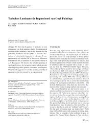
It is easy to remember how Chebyshev points are de ned: they are the
projections onto the interval [;11] of equally-spaced points (roots of unity)
along the unit circle jzj = 1 in the complex plane:
Figure 8.1.1. Chebyshev extreme points (N =8).
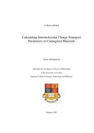
To the eye, Legendre points look much the same, although there is no
elementary geometrical de nition. Figure 8.1.2 illustrates the similarity:
Figure 8.1.2. Legendre vs. Chebyshev zeros.
As N !1, equispaced points are distributed with density
(x)= N
2
(a) N =5
(b) N =25
Equally spaced (8:1:2)

8.1. POLYNOMIAL INTERPOLATION TREFETHEN 1994 264
and Legendre or Chebyshev points|either zeros or extrema|have density
(x)=
N
p 1;x 2
Legendre, Chebyshev: (8:1:3)
Indeed, the density function (8.1.3) applies to point sets associated with any
Jacobi polynomials, of which Legendre and Chebyshev polynomials are special
cases.
Why is it a good idea to base spectral methods upon Chebyshev, Legendre,
and other irregular grids? We shall answer this question by addressing
a second, more fundamental question: why is it a good idea to interpolate a
function f(x) de ned on [;11] by a polynomial p N (x) rather than a trigonometric
polynomial, and why is it a good idea to use Chebyshev or Legendre
points rather than equally spaced points?
[The remainder of this section is just a sketch::: details to be supplied later.]
PHENOMENA
Trigonometric interpolation in equispaced points su ers from the Gibbs
phenomenon, due to Michelson and Gibbs at the turn of the twentieth century.
kf ; p N k = O(1) as N !1, even if f is analytic. One can try to get
around the Gibbs phenomenon by various tricks such as doubling the domain
and re ecting, but the price is high.
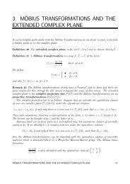
Polynomial interpolation in equally spaced points su ers from the Runge
phenomenon, due to Meray and Runge (Figure 8.1.3). kf ;p N k = O(2 N )|
much worse!
Polynomial interpolation in Legendre or Chebyshev points: kf ; p N k =
O(constant ;N ) if f is analytic (for some constant greater than 1). Even if
f is quite rough the errors will still go to zero provided f is, say, Lipschitz
continuous.

8.1. POLYNOMIAL INTERPOLATION TREFETHEN 1994 265
Figure 8.1.3. The Runge phenomenon.

8.1. POLYNOMIAL INTERPOLATION TREFETHEN 1994 266
FIRST EXPLANATION|EQUIPOTENTIAL CURVES
Think of the limiting point distribution (x), above, as a charge density
distribution a charge at position x is associated with a potential log jz ; xj.
Look at the equipotential curves of the resulting potential function (z)=
R 1;1 (x)logjz ;xjdx.
Theorem 8.1.
CONVERGENCE OF POLYNOMIAL INTERPOLANTS
In general, kf ; p N k!0 as N !1 in the largest region bounded by an
equipotential curve in which f is analytic. In particular:
For Chebyshev or Legendre points, or any other type of Gauss-Jacobi points,
convergence is guaranteed if f is analytic on [;11].
For equally spaced points, convergence is guaranteed if f is analytic in a
particular lens-shaped region containing (;11) (Figure 8.1.4).
Figure 8.1.4. Equipotential curves.

8.1. POLYNOMIAL INTERPOLATION TREFETHEN 1994 267
SECOND EXPLANATION|LEBESGUE CONSTANTS
De nition of Lebesgue constant:
N = kI Nk 1
where I N is the interpolation operator I N : f 7! p N . A small Lebesgue constant
means that the interpolation process is not much worse than best approximation:
kf ;p N k ( N +1)kf ;p N k (8:1:1)
where p N is the best (minimax, equiripple) approximation.
Theorem 8.2.
LEBESGUE CONSTANTS
Equispaced points: N 2N =eN log N.
p
Legendre points: N const N.
Chebyshev points: N const log N.
THIRD EXPLANATION|NUMBER OF POINTS PER WAVELENGTH
Consider approximation of, say, f N (x) = cos Nx as N !1. Thus f N
changes but the number of points per wavelength remains constant. Will the
error kf N ; p N k go to zero? The answer to this question tells us something
about the ability ofvarious kinds of spectral methods to resolve data.
Theorem 8.3.
POINTS PER WAVELENGTH
Equispaced points: convergence if there are at least 6 points per wavelength.
Chebyshev points: convergence if there are at least points per wavelength
on average.
We have to say \on average" because the grid is nonuniform. In fact, it
is =2 times less dense in the middle than the equally spaced grid with the
same number of points N (see (8.1.2) and (8.1.3)). Thus the second part of
the theorem says that we need at least 2 points per wavelength in the center
of the grid|the familiar Nyquist limit. See Figure 8.1.5. The rst part of
the theorem is mathematically valid, but of little value in practice because of
rounding errors.

8.2. CHEBYSHEV DIFFERENTIATION MATRICES TREFETHEN 1994 268
(a) Equally spaced points
(b) Chebyshev points
Figure 8.1.5. Error as a function of N in interpolation of cos Nx,
with ,hencethe number of points per wavelength, held xed.

8.2. CHEBYSHEV DIFFERENTIATION MATRICES TREFETHEN 1994 269
8.2. Chebyshev di erentiation matrices
[Just a sketch]
From now on \Chebyshev points" means Chebyshev extreme points.
Multiplication by the rst-order Chebyshev di erentiation matrix DN transforms a vector of data at the Chebyshev points into approximate derivatives
at those points:
2 3 2 3
v0 w0 D N
6
4
.
v N
7
5 =
6
4
.
w N
As usual, the implicit de nition of D N is as follows:
CHEBYSHEV SPECTRAL DIFFERENTIATION BY POLYNOMIAL INTERPOLA-
TION.
(1) Interpolate v by a polynomial q(x)=q N (x)
(2) Di erentiate the interpolant atthe grid points x j :
7
5 :
w j =(D Nv) j = q 0 (x j): (8:2:1)
Higher-order di erentiation matrices are de ned analogously. From this
de nition it is easy to work out the entries of D N in special cases. For N =1:
For N =2:
x =
2
3
7
x =
6
4 1
5 D1 =
;1
2
6
4
1
3
7
0
7
5
;1
D2 =
2
6
4
2 1
6 2 ;
4
1 2
1
2 ; 1 3
7
5:
2
3 2 ;2 1 2
3
7
1
2 0 ; 1 2
; 1 2 2 ; 3 7
5
2
:

8.2. CHEBYSHEV DIFFERENTIATION MATRICES TREFETHEN 1994 270
For N =3:
x =
2
6
4
1
1 2
; 1 2
3
7
5
D 3 =
2
6
4
19 6 ;4 4 3 ; 1 2
1 ; 1 3 ;1 1 3
; 1 3 1 1 3 ;1
1 ;1
2 ; 4 3 4 ; 19
6
These three examples illustrate an important fact, mentioned in the introduction
to this chapter: Chebyshev spectral di erentiation matrices are in general
not symmetric or skew-symmetric. A more general statement is that they are
not normal.* This is why stability analysis is di cult for spectral methods.
The reason they are not normal is that unlike nitedi erence di erentiation,
spectral di erentiation is not a translation-invariant process, but depends instead
on the same global interpolant atallpoints xj .
The general formula for D N is as follows. First, de ne
c i =
and of course analogously for c j . Then:
( 2 for i =0 or N,
1 for 1 i N ;1,
CHEBYSHEV SPECTRAL DIFFERENTIATION
3
7
5
:
(8:2:2)
Theorem 8.4. Let N 1 be any integer. The rst-order spectral di erentiation
matrix D N has entries
(D N) 00 = 2N 2 +1
6
(D N) jj = ;x j
2(1;x 2 j )
(D N) ij = c i
c j
(DN ) NN = ; 2N 2 +1
6
(;1) i+j
x i ;x j
for 1 j N ;1
for i 6= j:
Analogous formulas for D2 N can be found in Peyret (1986), Ehrenstein &
Peyret [ref?] and in Zang, Streett, and Hussaini, ICASE Report 89-13, 1989.
See also Canuto, Hussaini, Quarteroni &Zang.
*Recall that a normal matrix A is one that satis es AA T = A T A. Equivalently, A possesses an
orthogonal set of eigenvectors, which implies many desirable properties such as (A n )=kA n k =
kAk n for any n.

8.2. CHEBYSHEV DIFFERENTIATION MATRICES TREFETHEN 1994 271
A note of caution: D N is rarely used in exactly the form described in
Theorem 8.4, for boundary conditions will modify it slightly, and these depend
on the problem.
EXERCISES
. 8.2.1. Prove that for any N, DN is nilpotent: Dn N = 0 for a su ciently high integer n.

8.3. CHEBYSHEV DIFFERENTIATION BY THE FFT TREFETHEN 1994 272
8.3. Chebyshev di erentiation by the FFT
Polynomial interpolation in Chebyshev points is equivalent to trigonometric interpolation
in equally spaced points, and hence can be carried out by the FFT. The algorithm
described below has the optimal order O(N logN),* but we donotworry about achieving
the optimal constant factor. For more practical discussions, see Appendix B of the book by
Canuto, et al., and also P. N.Swarztrauber, \Symmetric FFTs," Math. Comp. 47 (1986),
323{346. Valuable additional references are the book The Chebyshev Polynomials by Rivlin
and Chapter 13 of P. Henrici, Applied and Computational Complex Analysis, 1986.
Consider three independent variables 2 R, x 2 [;11], and z 2 S, where S is the
complex unit circle fz : jzj =1g. They are related as follows:
which implies
z = e i x =Rez = 1 2 (z +z;1 ) = cos (8:3:1)
dx
d = ;sin = ;p 1;x 2 : (8:3:2)
See Figure 8.3.1. Note that there are two conjugate values z 2 S for each x 2 (;11), and
an in nite number of possible choices of .
;1 0 x
Figure 8.3.1. z, x, and .
*optimal, that is, so far as anyone knows as of 1994.
o*
o*
o*
z
z
1

8.3. CHEBYSHEV DIFFERENTIATION BY THE FFT TREFETHEN 1994 273
In generalization of the fact that the real part of z is x, the real part of z n (n 0)
is T n(x), the Chebyshev polynomial of degree n. This statement can be taken as a
de nitionofChebyshev polynomials:
T n (x)=Rez n = 1 2 (zn +z ;n ) = cos n (8:3:3)
where x and z and are, as always, implicitly related by (8.3.1).* It is clear that (8.3.3)
de nes T n (x) tobesome function of x, but it is not obvious that the function is a polynomial.
However, a calculation of the rst few cases makes it clear what is going on:
T0 (x) =1 2 (z0 +z ;0 )=1
T1 (x) =1 2 (z1 +z ;1 )=x
T2 (x) =1 2 (z2 +z ;2 )= 1 2 (z1 +z ;1 ) 2 ;1=2x 2 ;1
T3 (x) =1 2 (z3 +z ;3 )= 1 2 (z1 +z ;1 ) 3 ; 3 2 (z1 +z ;1 )=4x 3 ;3x:
In general, the Chebyshev polynomials are related by the three-term recurrence relation
T n+1 (x)= 1 2 (zn+1 +z ;n;1 )
= 1 2 (z1 +z ;1 )(z n +z ;n ); 1 2 (zn;1 +z ;n+1 )
=2xT n(x);T n;1(x):
By (8.3.2) and (8.3.3), the derivative ofT n(x) is
T 0
n(x)=;n sin n d n sin n
=
dx sin
(8:3:4)
(8:3:5)
: (8:3:6)
Thus just as x, z, and are equivalent, so are T n (x), z n , and cos n . By taking linear
combinations, we obtain three equivalent kinds of polynomials. A trigonometric polynomial
q( ) of degree N isa2 -periodic sum of complex exponentials in (or equivalently,
sines and cosines). Assuming that q( )isaneven function of , it can be written
NX
NX
q( )= 1 2 an (e
n=0
in +e ;in )= an cos n : (8:3:7)
n=0
A Laurent polynomial q(z) of degree N is a sum of negative and positive powers of z up
to degree N. Assuming q(z)=q(z) for z 2 S, it can be written
NX
q(z)= 1 2 an(z n=0
n +z ;n ): (8:3:8)
An algebraic polynomial q(x) of degree N is a polynomial in x of the usual kind, and we
can express it as a linear combination of Chebyshev polynomials:
NX
q(x)= anTn(x): (8:3:9)
n=0
*Equivalently, the Chebyshev polynomials can be de ned as a system of polynomials orthogonal on
[;1 1] with respect to the weight function (1;x 2 ) ;1=2 .

8.3. CHEBYSHEV DIFFERENTIATION BY THE FFT TREFETHEN 1994 274
The use of the same coe cients a n in (8.3.7){(8.3.9) is no accident, for all three of the
polynomials above are identical:
q( )=q(z)=q(x) (8:3:10)
where again, x and z and are implicitly related by (8.3.1). For this reason we hopetobe
forgiven the sloppy use of the same letter q in all three cases.
Finally, for any integer N 1, we de ne regular grids in the three variables as follows:
j
= j
N z j = ei j x j =Rez j = 1 2 (z j +z;1
j )=cos j (8:3:11)
for 0 j N. The points fx j g and fz j g were illustrated already in Figure 8.1.1. And now
we are ready to state the algorithm for Chebyshev di erentiation by the FFT.

8.3. CHEBYSHEV DIFFERENTIATION BY THE FFT TREFETHEN 1994 275
ALGORITHM FOR CHEBYSHEV DIFFERENTIATION
1. Given data fv j g de ned at the Chebyshev points fx j g, 0 j N, think of the same
data as being de ned at the equally spaced points f j g in [0 ].
2. (FFT) Find the coe cients fa ng of the trigonometric polynomial
that interpolates fv j g at f j g.
3. (FFT) Compute the derivative
dq
d
NX
q( )= an cos n (8:3:12)
n=0
NX
= ; nan sin n : (8:3:13)
n=0
4. Change variables to obtain the derivative with respect to x:
dq dq d
=
dx d dx =
NX
n=0
na n sin n
sin
NX
=
n=0
na n sin n
p 1;x 2
At x = 1, i.e. =0 , L'Hopital's rule gives the special values
NX
: (8:3:14)
dq
( 1) = ( 1)
dx
n=0
n n 2 an (8:3:15)
5. Evaluate the result at the Chebyshev points:
wj = dq
dx (xj ): (8:3:16)
Note that by (8.3.3), equation (8.3.12) can be interpreted as a linear combination of
Chebyshev polynomials, and by (8.3.6), equation (8.3.14) is the corresponding linear combination
of derivatives.* But of course the algorithmic content of the description above
relates to the variable, for in Steps 2 and 3, we have performed Fourier spectral di erentiation
exactly as in x7.3: discrete Fourier transform, multiply by i ,inverse discrete Fourier
transform. Only the use of sines and cosines rather than complex exponentials, and of n
instead of , has disguised the process somewhat.
*orofChebyshev polynomials Un(x) ofthe second kind.

8.3. CHEBYSHEV DIFFERENTIATION BY THE FFT TREFETHEN 1994 276
EXERCISES
. 8.3.1. Fourier and Chebyshev spectral di erentiation.
Write four brief, elegant Matlab programs for rst-order spectral di erentiation:
FDERIVM, CDERIVM: construct di erentiation matrices
FDERIV, CDERIV: di erentiate via FFT.
In the Fourier case, there are N equally spaced points x ;N=2 :::x N=2;1 (N even) in
[; ], and no boundary conditions. In the Chebyshev case, there are N Chebyshev points
x1:::x N in [;11) (N arbitrary), with a zero boundary condition at x =1. The e ect of
this boundary condition is that one removes the rst row and rst column from D N , leading
to a square matrix of dimension N instead of N +1.
You do not have toworry about computational e ciency (such as using an FFT of length
N rather than 2N in the Chebyshev case), but you are welcome to worry about it if you
like.
Experiment withyour programs to make suretheydi erentiate successfully. Of course, the
matrices can be used to check the FFT programs.
(a) Turn in a plot showing the function u(x) = cos(x=2) and its derivative computed by
FDERIV, for N = 32. Discuss the results.
(b) Turn in a plot showing the function u(x)=cos( x=2) and its derivative computed by
CDERIV, again for N = 32. Discuss the results.
(c) Plot the eigenvalues of D N for Fourier and Chebyshev spectral di erentiation with
N = 8, 16, 32, 64.

8.5. STABILITY TREFETHEN 1994 277
8.5. Stability
This section is not yet written. What follows is a copy of a paper of mine from K.
W. Morton and M. J. Baines, eds., Numerical Methods for Fluid Dynamics III, Clarendon
Press, Oxford, 1988.
Because of stability problems like those described in this paper, more and more attention
is currently being devoted to implicit time-stepping methods for spectral computations.
The associated linear algebra problems are generally solved by preconditioned matrix iterations,
sometimes including a multigrid iteration.
This paper was written before I was using the terminology of pseudospectra. Iwould
now summarize Section 5 of this paper bysaying that although the spectrum of the Legendre
spectral di erentiation matrix is of size (N)asN !1, the pseudospectra are of size (N 2 )
for any >0. The connection of pseudospectra with stability of the method of lines was
discussed in Sections 4.5{4.7.

8.5. STABILITY TREFETHEN 1994 278

8.5. STABILITY TREFETHEN 1994 279

8.5. STABILITY TREFETHEN 1994 280

8.5. STABILITY TREFETHEN 1994 281

8.5. STABILITY TREFETHEN 1994 282

8.5. STABILITY TREFETHEN 1994 283

8.5. STABILITY TREFETHEN 1994 284

8.5. STABILITY TREFETHEN 1994 285

8.5. STABILITY TREFETHEN 1994 286

8.5. STABILITY TREFETHEN 1994 287

8.5. STABILITY TREFETHEN 1994 288

8.5. STABILITY TREFETHEN 1994 289

8.5. STABILITY TREFETHEN 1994 290

8.5. STABILITY TREFETHEN 1994 291

8.5. STABILITY TREFETHEN 1994 292

8.5. STABILITY TREFETHEN 1994 293

8.5. STABILITY TREFETHEN 1994 294

8.5. STABILITY TREFETHEN 1994 295

8.5. STABILITY TREFETHEN 1994 296

8.5. STABILITY TREFETHEN 1994 297

8.6. SOME REVIEW PROBLEMS TREFETHEN 1994 297
8.6. Some review problems
EXERCISES
. 8.6.1. TRUE or FALSE? Give each answer together with at most two or three
sentences of explanation. The best possible explanation is a proof, a counterexample,
or the citation of a theorem in the text from which the answer follows. If you can't
do quite that well, try at least to give a convincing reason why the answer you have
chosen is the right one.In some cases a well-thought-out sketch will su ce.
(a) The Fourier transform of f(x) = exp(;x 4 ) has compact support.
(b) When you multiply a matrix by a vector on the right, i.e. Ax, the result is a
linear combination of the columns of that matrix.
(c) If an ODE initial-value problem with a smooth solution is solved by the fourthorder
Adams-Bashforth formula with step size k, and the missing starting values
v 1 , v 2 , v 3 are obtained by taking Euler steps with some step size k 0 , then in
general we will need k 0 = O(k 4 )tomaintain overall fourth-order accuracy.
(d) If a consistent nite di erence model of a well-posed linear initial-value problem
violates the CFL condition, it must be unstable.
(e) If you Fourier transform a function u 2 L 2 four times in a row, you end up with
u again, times a constant factor.
(f) If the function f(x)=(x 2 ;2x+26=25) ;1 is interpolated by a polynomial q N (x)
in N equally spaced points of [;11], then kf ;q N k 1 ! 0asN !1.
(g) e x = O(xe x=2 )asx !1.
(h) If a stable nite-di erence approximation to u t = u x with real coe cients has
order of accuracy 3, then the formula must be dissipative.
(i) If
A =
12 1
1
2
1
2
then kA n k

8.6. SOME REVIEW PROBLEMS TREFETHEN 1994 298
formula in t. For N =32, k =0:01 is a su ciently small time step to ensure
time-stability.
(l) The ODE initial-value problem u t = f(ut)=cos 2 u, u(0) = 1, 0 t 100, is
well-posed.
(m) In exact arithmetic and with exact starting values, the numerical approximations
computed by the linear multistep formula
v n+3 = 1 3 (vn+2 +v n+1 +v n )+ 2 3 k(f n+2 +f n+1 +f n )
are guaranteed to converge to the unique solution of a well-posed initial-value
problem in the limit k ! 0.
(n) If computers did not make rounding errors, wewould not need to study stability.
(o) The solution at time t =1 to u t = u x +u xx (x 2 R, initial data u(x0) = f(x)) is
the same as what you would get by rst di using the data f(x) according to the
equation u t = u xx, then translating the result leftward by one unit according to
the equation u t = u x.
(p) The discrete Fourier transform of a three-dimensional periodic set of data on an
N N N grid can be computed on a serial computer in O(N 3 logN) operations.
(q) The addition of numerical dissipation may sometimes increase the stability limit
of a nite di erence formula without a ecting the order of accuracy.
(r) For a nondissipative semidiscrete nite-di erence model (i.e., discrete space but
continuous time), phase velocity aswell as group velocity isawell-de ned quantity.
0 = vn 4 is a stable left-hand boundary condition for use with the leap frog
model of ut = ux with k=h =0:5.
(s) v n+1
(t) If a nite di erence model of a partial di erential equation is stable with k=h =
0 for some 0 > 0, then it is stable with k=h = for any 0.
(u) To solve the system of equations that results from a standard second-order
discretization of Laplace's equation on an N N N grid in three dimensions
by the obvious method of banded Gaussian elimination, without any clever
tricks, requires (N 7 ) operations on a serial computer.
(v) If u(xt) is a solution to u t = iu xx for x 2 R, then the 2-norm ku( t)k is independent
oft.
(w) In a method of lines discretization of a well-posed linear IVP, having the appropriate
eigenvalues t in the appropriate stability region is su cient but not
necessary for Lax-stability.
(x) Suppose a signal that's band-limited to frequencies in the range [;40kHz 40kHz]
is sampled 60,000 times a second, i.e., fast enough to resolve frequencies in the
range [;30kHz30kHz]. Then although some aliasing will occur, the information
in the range [;20kHz20kHz] remains uncorrupted.

8.7. TWO FINAL PROBLEMS TREFETHEN 1994 299
8.7. Two nal problems
EXERCISES
. 8.7.1. Equipotential curves. Write a short and elegant Matlab program to plot
equipotential curves in the plane corresponding to avector of point charges (interpolation
points) x 1 :::x N . Your program should simply sample N ;1P logjz ;x j j
on a grid, then produce a contour plot of the result. (See meshdom and contour.)
Turn in beautiful plots corresponding to (a) 6 equispaced points, (b) 6 Chebyshev
points, (c) 30 equispaced points, (d) 30 Chebyshev points. By all means play around
with 3D graphics, convergence and divergence of associated interpolation processes,
or other amusements if you're in the mood.
. 8.7.2. Fun with Chebyshev spectral methods. The starting point of this problem
is the Chebyshev di erentiation matrix of Exercise 8.3.1. It will be easiest to use
a program like CDERIVM from that exercise, which works with an explicit matrix
rather than the FFT. Be careful with boundary conditions you will want to square
the (N +1) (N +1) matrix rst before stripping o any rows or columns.
(a) Poisson equation in 1D. The function u(x)=(1;x 2 )e x satis es u( 1)=0 and
has second derivative u 00 (x)=;(1 + 4x + x 2 )e x . Thus it is the solution to the
boundary value problem
u xx = ;(1+4x+x 2 )e x x 2 [;11] u( 1)=0: (1)
Write a little Matlab program to solve (1) by aChebyshev spectral method and
produce a plot of the computed discrete solution values (N +1 discrete points in
[;11]) superimposed upon exact solution (a curve). Turn in the plot for N =6
and a table of the errors ucomputed(0);uexact(0) for N =2468. What can you
say about the rate of convergence?
(b) Poisson equation in 2D. Similarly, the function u(xy)=(1;x 2 )(1;y 2 )cos(x+y)
is the solution to the boundary value problem
u xx+u yy = xy 2 [;11] u(x 1) = u( 1y)=0: (2)
Write a Matlab program to solve (2) by aChebyshev spectral method involving
a grid of (N ; 1) 2 interior points. You may nd that the Matlab command
KRON comes in handy for this purpose. You don't have to produce a plot of
the computed solution, but do turn in a table of ucomputed(00);uexact(00) for
N =2468. How does the rate of convergence look?
(c) Heat equation in 1D. Back to1D now. Suppose you have the problem
u t = u xx u( 1t)=0 u(x0) = (1;x 2 )e x : (3)

8.7. TWO FINAL PROBLEMS TREFETHEN 1994 300
At what time t c does max x2[;11] u(xt) rst fall below1? Figure out the answer
to at least 2 digits of relative precision. Then describe what you would do if I
asked for 12 digits.