Download Chapters 3-6 (.PDF) - ODBMS

38 6. DISCUSSION—POWER LAWS AND DEVIATIONS
where μ and σ are parameters and A(μ, σ ) is a constant (used for normalization if y(x) is a
probability distribution). The DGX distribution has been used to fit the degree distribution of a
bipartite “clickstream” graph linking websites and users (Figure 2.2(c)), telecommunications, and
other data.
6.2.3 DOUBLY-PARETO LOGNORMAL (DPLN )
Another deviation is well modeled by the so-called Doubly Pareto Lognormal (dPln). Mitzenmacher
[210] obtained good fits for file size distributions using dPln. Seshadri et al. [245] studied
the distribution of phone calls per customer, and also found it to be a good fit. We will describe the
results of Seshadri et al. below.
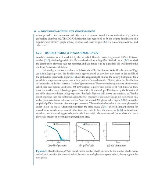
Informally, a random variable that follows the dPln distribution looks like the plots of Figure
6.1: in log-log scales, the distribution is approximated by two lines that meet in the middle of
the plot. More specifically, Figure 6.1 shows the empirical pdf (that is, the density histogram) for a
switch in a telephone company, over a time period of several months. Plot (a) gives the distribution
of the number of distinct partners (“callees”) per customer.The overwhelming majority of customers
called only one person; until about 80-100 “callees,” a power law seems to fit well; but after that,
there is a sudden drop, following a power-law with a different slope. This is exactly the behavior of
the dPln: piece-wise linear, in log-log scales. Similarly, Figure 6.1(b) shows the empirical pdf for the
count of phone calls per customer: again, the vast majority of customers make just one phone call,
with a piece-wise linear behavior, and the “knee” at around 200 phone calls. Figure 6.1(c) shows the
empirical pdf for the count of minutes per customer.The qualitative behavior is the same: piece-wise
linear, in log-log scales. Additional plots from the same source ([245]) showed similar behavior for
several other switches and several other time intervals. In fact, the dataset in [245] included four
switches, over month-long periods; each switch recorded calls made to and from callers who were
physically present in a contiguous geographical area.
PDF
10 -2
10 -4
10 -6
10 0
10 1
Data
Fitted DPLN[2.8, 0.01, 0.35, 3.8]
10 2
Partners
10 3
10 4
PDF
10 -2
10 -4
10 -6
10 0
10 2
Data
Fitted DPLN[2.8, 0.01, 0.55, 5.6]
10 3
Calls
10 4
10 5
PDF
10 -2
10 -4
10 -6
Data
Fitted DPLN[2.5, 0.01, 0.45, 6.5]
10 2
Duration
(a) pdf of partners (b) pdf of calls (c) pdf of minutes
Figure 6.1: Results of using dPln to model. (a) the number of call-partners, (b) the number of calls made,
and (c) total duration (in minutes) talked, by users at a telephone-company switch, during a given the
time period.
10 4