Download Chapters 3-6 (.PDF) - ODBMS

For each customer, the following counts were computed:
6.2. DEVIATIONS FROM POWER LAWS 39
Partners: The total number of unique callers and callees associated with every user. Note that
this is essentially the degree of nodes in the (undirected and unweighted) social graph, which
has an edge between two users if either called the other.
Calls: The total number of calls made or received by each user. In graph theoretic terms, this
is the weighted degree in the social graph where the weight of an edge between two users is
equal to the number of calls that involved them both.
Duration: The total duration of calls for each customer in minutes. This is the weighted
degree in the social graph where the weight of the edge between two users is the total duration
of the calls between them.
The dPln Distribution For the intuition and the fitting of the dPln distribution, see the work of
Reed [238]. Here, we mention only the highlights.
If a random variable X follows the four-parameter dPln distribution dPln(α, β, ν, τ), then
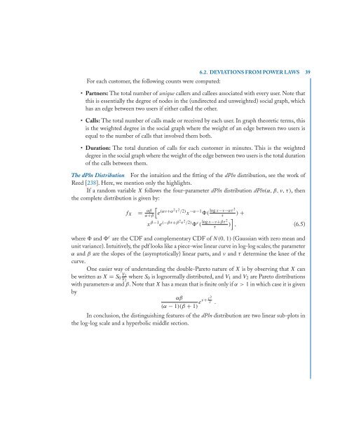
the complete distribution is given by:
fX = αβ
α+β e (αν+α2τ 2 /2) x−α−1 log x−ν−ατ
( 2
τ
xβ−1e (−βτ+β2τ 2 /2) c log x−ν+βτ
( 2
τ )
) +
, (6.5)
where and c are the CDF and complementary CDF of N(0, 1) (Gaussian with zero mean and
unit variance). Intuitively, the pdf looks like a piece-wise linear curve in log-log scales; the parameter
α and β are the slopes of the (asymptotically) linear parts, and ν and τ determine the knee of the
curve.
One easier way of understanding the double-Pareto nature of X is by observing that X can
be written as X = S0 V1
V2 where S0 is lognormally distributed, and V1 and V2 are Pareto distributions
with parameters α and β. Note that X has a mean that is finite only if α>1 in which case it is given
by
αβ
τ2
eν+ 2 .
(α − 1)(β + 1)
In conclusion, the distinguishing features of the dPln distribution are two linear sub-plots in
the log-log scale and a hyperbolic middle section.