Differential Equation Solving With DSolve - Wolfram Research
Differential Equation Solving With DSolve - Wolfram Research
Differential Equation Solving With DSolve - Wolfram Research

You also want an ePaper? Increase the reach of your titles
YUMPU automatically turns print PDFs into web optimized ePapers that Google loves.
<strong>Wolfram</strong><br />
Mathematica ® Tutorial Collection<br />
DIFFERENTIAL EQUATION<br />
SOLVING WITH DSOLVE
For use with <strong>Wolfram</strong> Mathematica ® 7.0 and later.<br />
For the latest updates and corrections to this manual:<br />
visit reference.wolfram.com<br />
For information on additional copies of this documentation:<br />
visit the Customer Service website at www.wolfram.com/services/customerservice<br />
or email Customer Service at info@wolfram.com<br />
Comments on this manual are welcomed at:<br />
comments@wolfram.com<br />
Content authored by:<br />
Devendra Kapadia<br />
Printed in the United States of America.<br />
15 14 13 12 11 10 9 8 7 6 5 4 3 2<br />
©2008 <strong>Wolfram</strong> <strong>Research</strong>, Inc.<br />
All rights reserved. No part of this document may be reproduced or transmitted, in any form or by any means,<br />
electronic, mechanical, photocopying, recording or otherwise, without the prior written permission of the copyright<br />
holder.<br />
<strong>Wolfram</strong> <strong>Research</strong> is the holder of the copyright to the <strong>Wolfram</strong> Mathematica software system ("Software") described<br />
in this document, including without limitation such aspects of the system as its code, structure, sequence,<br />
organization, “look and feel,” programming language, and compilation of command names. Use of the Software unless<br />
pursuant to the terms of a license granted by <strong>Wolfram</strong> <strong>Research</strong> or as otherwise authorized by law is an infringement<br />
of the copyright.<br />
<strong>Wolfram</strong> <strong>Research</strong>, Inc. and <strong>Wolfram</strong> Media, Inc. ("<strong>Wolfram</strong>") make no representations, express,<br />
statutory, or implied, with respect to the Software (or any aspect thereof), including, without limitation,<br />
any implied warranties of merchantability, interoperability, or fitness for a particular purpose, all of<br />
which are expressly disclaimed. <strong>Wolfram</strong> does not warrant that the functions of the Software will meet<br />
your requirements or that the operation of the Software will be uninterrupted or error free. As such,<br />
<strong>Wolfram</strong> does not recommend the use of the software described in this document for applications in<br />
which errors or omissions could threaten life, injury or significant loss.<br />
Mathematica, MathLink, and MathSource are registered trademarks of <strong>Wolfram</strong> <strong>Research</strong>, Inc. J/Link, MathLM,<br />
.NET/Link, and webMathematica are trademarks of <strong>Wolfram</strong> <strong>Research</strong>, Inc. Windows is a registered trademark of<br />
Microsoft Corporation in the United States and other countries. Macintosh is a registered trademark of Apple<br />
Computer, Inc. All other trademarks used herein are the property of their respective owners. Mathematica is not<br />
associated with Mathematica Policy <strong>Research</strong>, Inc.
Contents<br />
Introduction to <strong>Differential</strong> <strong>Equation</strong> <strong>Solving</strong> with <strong>DSolve</strong> . . . . . . . . . . . . . . . . . . . . . . 1<br />
Classification of <strong>Differential</strong> <strong>Equation</strong>s . . . . . . . . . . . . . . . . . . . . . . . . . . . . . . . . . . . . . . . . . . . 7<br />
Ordinary <strong>Differential</strong> <strong>Equation</strong>s (ODEs) . . . . . . . . . . . . . . . . . . . . . . . . . . . . . . . . . . . . . . . . . . 11<br />
Overview of ODEs . . . . . . . . . . . . . . . . . . . . . . . . . . . . . . . . . . . . . . . . . . . . . . . . . . . . . . . . . . . . . . 11<br />
First-Order ODEs . . . . . . . . . . . . . . . . . . . . . . . . . . . . . . . . . . . . . . . . . . . . . . . . . . . . . . . . . . . . . . . 12<br />
Linear Second-Order ODEs . . . . . . . . . . . . . . . . . . . . . . . . . . . . . . . . . . . . . . . . . . . . . . . . . . . . . . 24<br />
Nonlinear Second-Order ODEs . . . . . . . . . . . . . . . . . . . . . . . . . . . . . . . . . . . . . . . . . . . . . . . . . . 33<br />
Higher-Order ODEs . . . . . . . . . . . . . . . . . . . . . . . . . . . . . . . . . . . . . . . . . . . . . . . . . . . . . . . . . . . . . 36<br />
Systems of ODEs . . . . . . . . . . . . . . . . . . . . . . . . . . . . . . . . . . . . . . . . . . . . . . . . . . . . . . . . . . . . . . . 42<br />
Lie Symmetry Methods for <strong>Solving</strong> Nonlinear ODEs . . . . . . . . . . . . . . . . . . . . . . . . . . . . . 50<br />
Partial <strong>Differential</strong> <strong>Equation</strong>s (PDEs) . . . . . . . . . . . . . . . . . . . . . . . . . . . . . . . . . . . . . . . . . . . . . 55<br />
Introduction to PDEs . . . . . . . . . . . . . . . . . . . . . . . . . . . . . . . . . . . . . . . . . . . . . . . . . . . . . . . . . . . 55<br />
First-Order PDEs . . . . . . . . . . . . . . . . . . . . . . . . . . . . . . . . . . . . . . . . . . . . . . . . . . . . . . . . . . . . . . . . 56<br />
Second-Order PDEs . . . . . . . . . . . . . . . . . . . . . . . . . . . . . . . . . . . . . . . . . . . . . . . . . . . . . . . . . . . . . 66<br />
<strong>Differential</strong>-Algebraic <strong>Equation</strong>s (DAEs) . . . . . . . . . . . . . . . . . . . . . . . . . . . . . . . . . . . . . . . . . 70<br />
Introduction to DAEs . . . . . . . . . . . . . . . . . . . . . . . . . . . . . . . . . . . . . . . . . . . . . . . . . . . . . . . . . . . 70<br />
Examples of DAEs . . . . . . . . . . . . . . . . . . . . . . . . . . . . . . . . . . . . . . . . . . . . . . . . . . . . . . . . . . . . . . 71<br />
Initial and Boundary Value Problems . . . . . . . . . . . . . . . . . . . . . . . . . . . . . . . . . . . . . . . . . . . . . 76<br />
Introduction to Initial and Boundary Value Problems . . . . . . . . . . . . . . . . . . . . . . . . . . . 76<br />
Linear IVPs and BVPs . . . . . . . . . . . . . . . . . . . . . . . . . . . . . . . . . . . . . . . . . . . . . . . . . . . . . . . . . . . 77<br />
Nonlinear IVPs and BVPs . . . . . . . . . . . . . . . . . . . . . . . . . . . . . . . . . . . . . . . . . . . . . . . . . . . . . . . 82<br />
IVPs with Piecewise Coefficients . . . . . . . . . . . . . . . . . . . . . . . . . . . . . . . . . . . . . . . . . . . . . . . . 85<br />
Working with <strong>DSolve</strong>~A User’s Guide . . . . . . . . . . . . . . . . . . . . . . . . . . . . . . . . . . . . . . . . . . . . 89<br />
Introduction . . . . . . . . . . . . . . . . . . . . . . . . . . . . . . . . . . . . . . . . . . . . . . . . . . . . . . . . . . . . . . . . . . . . 89<br />
Setting Up the Problem . . . . . . . . . . . . . . . . . . . . . . . . . . . . . . . . . . . . . . . . . . . . . . . . . . . . . . . . . 90<br />
Verification of the Solution . . . . . . . . . . . . . . . . . . . . . . . . . . . . . . . . . . . . . . . . . . . . . . . . . . . . . 94<br />
Plotting the Solution . . . . . . . . . . . . . . . . . . . . . . . . . . . . . . . . . . . . . . . . . . . . . . . . . . . . . . . . . . . . 98<br />
The GenerateParameters Options . . . . . . . . . . . . . . . . . . . . . . . . . . . . . . . . . . . . . . . . . . . . . . . 102<br />
Symbolic Parameters and Inexact Quantities . . . . . . . . . . . . . . . . . . . . . . . . . . . . . . . . . . . 104<br />
Is the Problem Well-Posed? . . . . . . . . . . . . . . . . . . . . . . . . . . . . . . . . . . . . . . . . . . . . . . . . . . . . 108<br />
References . . . . . . . . . . . . . . . . . . . . . . . . . . . . . . . . . . . . . . . . . . . . . . . . . . . . . . . . . . . . . . . . . . . . . . . . . 111
Introduction to <strong>Differential</strong> <strong>Equation</strong><br />
<strong>Solving</strong> with <strong>DSolve</strong><br />
The Mathematica function <strong>DSolve</strong> finds symbolic solutions to differential equations. (The Mathe-<br />
matica function N<strong>DSolve</strong>, on the other hand, is a general numerical differential equation<br />
solver.) <strong>DSolve</strong> can handle the following types of equations:<br />
† Ordinary <strong>Differential</strong> <strong>Equation</strong>s (ODEs), in which there is a single independent variable t and<br />
one or more dependent variables xiHtL. <strong>DSolve</strong> is equipped with a wide variety of techniques<br />
for solving single ODEs as well as systems of ODEs.<br />
† Partial <strong>Differential</strong> <strong>Equation</strong>s (PDEs), in which there are two or more independent variables<br />
and one dependent variable. Finding exact symbolic solutions of PDEs is a difficult problem,<br />
but <strong>DSolve</strong> can solve most first-order PDEs and a limited number of the second-order PDEs<br />
found in standard reference books.<br />
† <strong>Differential</strong>-Algebraic <strong>Equation</strong>s (DAEs), in which some members of the system are differential<br />
equations and the others are purely algebraic, having no derivatives in them. As with<br />
PDEs, it is difficult to find exact solutions to DAEs, but <strong>DSolve</strong> can solve many examples of<br />
such systems that occur in applications.<br />
<strong>DSolve</strong>@eqn,y@xD,xD solve a differential equation for y@xD<br />
<strong>DSolve</strong>@8eqn 1 ,eqn 2 ,…
2 <strong>Differential</strong> <strong>Equation</strong> <strong>Solving</strong> with <strong>DSolve</strong><br />
You can pick out a specific solution by using ê. (ReplaceAll).<br />
In[2]:= y@xD ê. <strong>DSolve</strong>@8y'@xD ã y@xD
The solution to this differential equation is given as a pure function.<br />
In[5]:= eqn = 8y'@xD ã y@xD^2, y@0D ã 1<br />
1 - x<br />
This verifies the solution.<br />
In[7]:= eqn ê. sol<br />
Out[7]= 88True, True
4 <strong>Differential</strong> <strong>Equation</strong> <strong>Solving</strong> with <strong>DSolve</strong><br />
While general solutions to ordinary differential equations involve arbitrary constants, general<br />
solutions to partial differential equations involve arbitrary functions. <strong>DSolve</strong> labels these arbi-<br />
trary functions as C@iD.<br />
Here is the general solution to a linear first-order PDE. In the solution, C@1D labels an arbitrary<br />
function of -x+y<br />
x y .<br />
In[12]:= eqn = x^2 * D@u@x, yD, xD + y^2 * D@u@x, yD, yD - Hx + yL * u@x, yD;<br />
sol = <strong>DSolve</strong>@eqn ã 0, u, 8x, y<br />
x y<br />
This obtains a particular solution to the PDE for a specific choice of C@1D.<br />
In[14]:= fn = u@x, yD ê. sol@@1DD ê. 8C@1D@t_D Ø Sin@t^2D + Ht ê 10L<<br />
Out[14]= -x y<br />
-x + y H-x + yL2<br />
+ SinB F<br />
10 x y<br />
x 2 y 2<br />
Here is a plot of the surface for this solution.<br />
In[15]:= Plot3D@fn, 8x, -5, 5
This verifies the solutions.<br />
In[18]:= Simplify@eqns ê. solD<br />
Out[18]= 88True, True, True, True
6 <strong>Differential</strong> <strong>Equation</strong> <strong>Solving</strong> with <strong>DSolve</strong><br />
The author hopes that these <strong>Differential</strong> <strong>Equation</strong> <strong>Solving</strong> with <strong>DSolve</strong> tutorials will be useful in<br />
acquiring a basic knowledge of <strong>DSolve</strong> and also serve as a ready reference for information on<br />
more advanced topics.
Classification of <strong>Differential</strong> <strong>Equation</strong>s<br />
While differential equations have three basic types~ordinary (ODEs), partial (PDEs), or differen-<br />
tial-algebraic (DAEs), they can be further described by attributes such as order, linearity, and<br />
degree. The solution method used by <strong>DSolve</strong> and the nature of the solutions depend heavily on<br />
the class of equation being solved.<br />
The order of a differential equation is the order of the highest derivative in the equation.<br />
This is a first-order ODE because its highest derivative is of order 1.<br />
In[1]:= <strong>DSolve</strong>@x^2 H1 - x^2L * y'@xD ã Hx - 3 x^3 - y@xDL y@xD, y@xD, xD<br />
-x + x<br />
Out[1]= ::y@xD Ø<br />
3<br />
>><br />
C@1D - Log@xD<br />
Here is the general solution to a fourth-order ODE.<br />
In[2]:= <strong>DSolve</strong>@y''''@xD - 16 * y@xD ã x^2, y@xD, xD<br />
Out[2]= ::y@xD Ø - x2<br />
16<br />
+ ‰ 2 x C@1D + ‰ -2 x C@3D + C@2D Cos@2 xD + C@4D Sin@2 xD>><br />
A differential equation is linear if the equation is of the first degree in y and its derivatives, and<br />
if the coefficients are functions of the independent variable.<br />
This is a nonlinear second-order ODE that represents the motion of a circular pendulum. It is<br />
nonlinear because Sin@y@xDD is not a linear function of y@xD. The Solve::ifun warning<br />
message appears because Solve uses JacobiAmplitude (the inverse of EllipticF) to find<br />
an expression for y@xD.<br />
In[3]:= sol = <strong>DSolve</strong>@y''@xD + 3 * Sin@y@xDD ã 0, y, xD<br />
<strong>Differential</strong> <strong>Equation</strong> <strong>Solving</strong> with <strong>DSolve</strong> 7<br />
Solve::ifun :<br />
Inverse functions are being used by Solve, so some solutions may not be found; use Reduce for<br />
complete solution information. à<br />
Out[3]= ::y Ø FunctionB8x,<br />
6 + C@1D<br />
:y Ø FunctionB8x><br />
6 + C@1D
8 <strong>Differential</strong> <strong>Equation</strong> <strong>Solving</strong> with <strong>DSolve</strong><br />
This plots the solutions. The discontinuity in the graphs at x = -3 results from the choice of<br />
inverse functions used by Solve.<br />
In[4]:= Plot@8y@xD ê. sol@@1DD ê. 8C@1D Ø -1, C@2D Ø 3
Here, x 2 is added to the right-hand side of the previous equation, making the new equation<br />
inhomogeneous. The general solution to this new equation is the sum of the previous solution<br />
and a particular integral.<br />
In[8]:= sol2 = <strong>DSolve</strong>@eqn ã x^2, y@xD, xD<br />
1124 + 1050 x + 441 x2<br />
Out[8]= ::y@xD Ø<br />
9261<br />
+ ‰ -7 x C@1D + ‰ x C@2D + ‰ 3 x C@3D>><br />
When the coefficients of an ODE depend on x, the ODE is said to have variable coefficients.<br />
Since equations with variable coefficients that are rational functions of x have singularities that<br />
are easily classified, there are sophisticated algorithms available for solving them.<br />
The coefficients of this equation are rational functions of x.<br />
In[9]:= sol =<br />
<strong>DSolve</strong>@8y''@xD - HH1 ê xL - H3 ê H16 x^2LLL * y@xD ã 0, y@1D ã 1, y'@1D ã 4><br />
There is a close relationship between functions and differential equations. Starting with a function<br />
of almost any type, it is possible to construct a differential equation satisfied by that function.<br />
Conversely, any differential equation gives rise to one or more functions, in the form of<br />
solutions to that equation. In fact, many special functions from classical analysis have their<br />
origins in the solution of differential equations. Mathieu functions are one such class of special<br />
functions. Mathieu was interested in studying the vibrations of elliptical membranes. The eigenfunctions<br />
for the wave equation that describes this motion are given by products of Mathieu<br />
functions.<br />
This linear second-order ODE with rational coefficients has a general solution given by Mathieu<br />
functions.<br />
In[10]:= <strong>DSolve</strong>@Ht - 1L Ht + 1L * y''@tD + t * y'@tD + H-2 - 6 * t^2L * y@tD ã 0, y@tD, tD<br />
Out[10]= ::y@tD Ø C@1D MathieuCB5, - 3<br />
, ArcCos@tDF + C@2D MathieuSB5, -<br />
2<br />
3<br />
, ArcCos@tDF>><br />
2<br />
The presence of ArcCos@tD in the previous solution suggests that the equation can be given a<br />
simpler form using trigonometric functions. This is the form in which these equations were<br />
introduced by Mathieu in 1868.<br />
In[11]:= <strong>DSolve</strong>@y''@xD + H3 Cos@2 xD + 5L y@xD == 0, y, xD<br />
Out[11]= ::y Ø FunctionB8x><br />
2<br />
<strong>Differential</strong> <strong>Equation</strong> <strong>Solving</strong> with <strong>DSolve</strong> 9
10 <strong>Differential</strong> <strong>Equation</strong> <strong>Solving</strong> with <strong>DSolve</strong><br />
This plots the surface for a particular product of solutions to this equation.<br />
In[12]:= Plot3DBMathieuCB5, - 3<br />
3<br />
, xF * MathieuSB5, - , yF, 8x, -3, 3
Ordinary <strong>Differential</strong> <strong>Equation</strong>s (ODEs)<br />
Overview of Ordinary <strong>Differential</strong> <strong>Equation</strong>s (ODEs)<br />
There are four major areas in the study of ordinary differential equations that are of interest in<br />
pure and applied science.<br />
<strong>Differential</strong> <strong>Equation</strong> <strong>Solving</strong> with <strong>DSolve</strong> 11<br />
† Exact solutions, which are closed-form or implicit analytical expressions that satisfy the<br />
given problem.<br />
† Numerical solutions, which are available for a wider class of problems, but are typically only<br />
valid over a limited range of the independent variables.<br />
† Qualitative theory, which is concerned with the global properties of solutions and is particularly<br />
important in the modern approach to dynamical systems.<br />
† Existence and uniqueness theorems, which guarantee that there are solutions with certain<br />
desirable properties provided a set of conditions is fulfilled by the differential equation.<br />
Of these four areas, the study of exact solutions has the longest history, dating back to the<br />
period just after the discovery of calculus by Sir Isaac Newton and Gottfried Wilhelm von Leib-<br />
niz. The following table introduces the types of equations that can be solved by <strong>DSolve</strong>.
12 <strong>Differential</strong> <strong>Equation</strong> <strong>Solving</strong> with <strong>DSolve</strong><br />
name of equation general form date of discovery mathematician<br />
Separable y £ HxL f HxL gHyL 1691 G. Leibniz<br />
Homogeneous y £ HxL f J x<br />
N 1691 G. Leibniz<br />
yHxL<br />
Linear first-order ODE y £ HxL + PHxL yHxL QHxL 1694 G. Leibniz<br />
Bernoulli y £ HxL + PHxL yHxL QHxL 1695 James Bernoulli<br />
Riccati y £ HxL f HxL + gHxL yHxL + hHxL yHxL 2<br />
Exact first-order ODE M d x + N d y 0 with ∂M<br />
∂y<br />
= ∂N<br />
∂x<br />
1724 Count Riccati<br />
1734 L. Euler<br />
Clairaut yHxL x y £ HxL + f Hy £ HxLL 1734 A-C. Clairaut<br />
Linear with constant<br />
coefficients<br />
y HnL HxL + an-1 y Hn-1L HxL + … + a0 yHxL PHxL<br />
with a1 constant<br />
Hypergeometric xH1 - xL y ££ HxL + Hc - Ha + b + 1L xL y £ HxL -<br />
a b yHxL 0<br />
1743 L. Euler<br />
1769 L. Euler<br />
Legendre I1 - x 2 M y ££ HxL - 2 x y £ HxL + nHn + 1L yHxL = 0 1785 M. Legendre<br />
Bessel x 2 y ££ HxL + x y £ HxL + Ix 2 - n 2 M y HxL = 0 1824 F. Bessel<br />
Mathieu y ££ HxL + Ha - 2 q cosH2 xLL yHxL = 0 1868 E. Mathieu<br />
Abel y £ HxL f HxL + gHxL yHxL + hHxL yHxL 2 +<br />
k HxL yHxL 3<br />
Chini y £ HxL f HxL + g HxL y HxL + h HxL y HxL n<br />
1834 N. H. Abel<br />
1924 M. Chini<br />
Examples of ODEs belonging to each of these types are given in other tutorials (clicking a link in<br />
the table will bring up the relevant examples).<br />
First-Order ODEs<br />
Straight Integration<br />
This equation is solved by simply integrating the right-hand side with respect to x.<br />
In[1]:= sol = <strong>DSolve</strong>@y'@xD ã x^2 * Sin@xD + Sqrt@1 + x^2D, y, xD<br />
Out[1]= ::y Ø FunctionB8x>
Here is a plot of the integral curves for different values of the arbitrary constant C@1D.<br />
In[2]:= tab = Table@y@xD ê. sol@@1DD ê. 8C@1D -> k
14 <strong>Differential</strong> <strong>Equation</strong> <strong>Solving</strong> with <strong>DSolve</strong><br />
The solution to this equation is given as an InverseFunction object, in order to get an<br />
explicit expression for y@xD.<br />
In[3]:= sol = <strong>DSolve</strong>By £ @xD ã<br />
x 2<br />
9 - x 2 Log@y@xDD * Sin@y@xDD<br />
, y@xD, xF<br />
InverseFunction::ifun : Inverse functions are being used. Values may be lost for multivalued inverses. à<br />
InverseFunction::ifun : Inverse functions are being used. Values may be lost for multivalued inverses. à<br />
Solve::tdep :<br />
The equations appear to involve the variables to be solved for in an essentially non-algebraic way. à<br />
Out[3]= ::y@xD Ø InverseFunction@CosIntegral@Ò1D - Cos@Ò1D Log@Ò1D &DB<br />
-Â 1<br />
-3 + x x 3 + x + 9 ArcSinhB<br />
-3 + x<br />
F + C@1DF>><br />
2<br />
6<br />
Homogeneous <strong>Equation</strong>s<br />
Here is a homogeneous equation in which the total degree of both the numerator and the<br />
denominator of the right-hand side is 2. The two parts of the solution list give branches of the<br />
integral curves in the form y = f HxL.<br />
In[1]:= eqn = y'@xD ã -Hx^2 - 3 y@xD^2L ê Hx * y@xDL;<br />
sol = <strong>DSolve</strong>@eqn, y, xD<br />
Out[2]= ::y Ø FunctionB8x, :y Ø FunctionB8x><br />
This plots both branches together, showing the complete integral curves y 2 C@1D x 6 + x2<br />
2 for<br />
several values of C@1D.<br />
In[3]:= tab1 = Table@y@xD ê. sol@@1DD ê. C@1D Ø k, 8k, 0, 3, 0.5
If an initial condition is specified, <strong>DSolve</strong> picks the branch that passes through the initial point.<br />
The <strong>DSolve</strong>::bvnul message indicates that one branch of the general solution (the lower<br />
branch in the previous graph) did not give a solution satisfying the given initial condition<br />
y@1D ã 3.<br />
In[6]:= <strong>DSolve</strong>@8eqn, y@1D ã 3><br />
The following is a linear first-order ODE because both y@xD and y £ @xD occur in it with power 1 and<br />
y £ @xD is the highest derivative. Note that the solution contains the imaginary error function Erfi.<br />
In[1]:= <strong>DSolve</strong>@y'@xD + x * y@xD ã Exp@3 xD, y@xD, xD<br />
x2<br />
9 x2<br />
- - -<br />
Out[1]= ::y@xD Ø ‰ 2 C@1D + ‰ 2 2<br />
p<br />
2<br />
3 + x<br />
ErfiB F>><br />
2<br />
Here is the solution for a more general linear first-order ODE. The K variables are used as<br />
dummy variables for integration. The Erfi term in the previous example comes from the<br />
integral in the second term of the general solution as follows.<br />
In[2]:= sol = <strong>DSolve</strong>@y'@xD + y@xD ã Q@xD, y@xD, xD<br />
Out[2]= ::y@xD Ø ‰ -x C@1D + ‰ -x ‡ 1<br />
x<br />
‰ K@1D Q@K@1DD „ K@1D>><br />
A more traditional form of the solution can be obtained by replacing K@1D with a variable such<br />
as t.<br />
In[3]:= sol ê. 8K@1D Ø t<<br />
Out[3]= ::y@xD Ø ‰ -x C@1D + ‰ -x ‡ 1<br />
x<br />
‰ t Q@tD „ t>><br />
Inverse Linear <strong>Equation</strong>s<br />
It may happen that a given ODE is not linear in yHxL but can be viewed as a linear ODE in xHyL. In<br />
this case, it is said to be an inverse linear ODE.<br />
<strong>Differential</strong> <strong>Equation</strong> <strong>Solving</strong> with <strong>DSolve</strong> 15
16 <strong>Differential</strong> <strong>Equation</strong> <strong>Solving</strong> with <strong>DSolve</strong><br />
This is a inverse linear ODE. It is constructed by interchanging x and y in an earlier example.<br />
In[1]:= <strong>DSolve</strong>@y'@xD ã 1 ê H-x * y@xD + Exp@3 * y@xDDL, y@xD, xD<br />
Solve::tdep :<br />
The equations appear to involve the variables to be solved for in an essentially non-algebraic way. à<br />
1<br />
-<br />
Out[1]= SolveBx ã ‰ 2 y@xD2<br />
9 y@xD2<br />
- -<br />
C@1D + ‰ 2 2<br />
Bernoulli <strong>Equation</strong>s<br />
p<br />
2<br />
3 + y@xD<br />
ErfiB F, y@xDF<br />
2<br />
A Bernoulli equation is a first-order equation of the form<br />
y £ HxL + PHxL yHxL QHxLyHxL n .<br />
The problem of solving equations of this type was posed by James Bernoulli in 1695. A year<br />
later, in 1696, G. Leibniz showed that it can be reduced to a linear equation by a change of<br />
variable.<br />
Here is an example of a Bernoulli equation.<br />
In[1]:= eqn = y'@xD + 11 x * y@xD ã x^3 * y@xD^3<br />
Out[1]= 11 x y@xD + y £ @xD ã x 3 y@xD 3<br />
In[2]:= sol = <strong>DSolve</strong>@eqn, y, xD<br />
Out[2]= ::y Ø FunctionB8x, :y Ø FunctionB8x>
Here is an example of a Bernoulli equation with n = 5. The solution has four branches.<br />
In[4]:= <strong>DSolve</strong>@3 x * y'@xD - 7 x * Log@xD * y@xD^5 - y@xD ã 0, y@xD, xD<br />
Out[4]= ::y@xD Ø -<br />
:y@xD Ø<br />
Riccati <strong>Equation</strong>s<br />
7 1ë4 x 1ë3<br />
I12 x 7ë3 + 7 C@1D - 28 x 7ë3 Log@xDM 1ë4<br />
 7 1ë4 x 1ë3<br />
I12 x 7ë3 + 7 C@1D - 28 x 7ë3 Log@xDM 1ë4<br />
>, :y@xD Ø -<br />
>, :y@xD Ø<br />
A Riccati equation is a first-order equation of the form<br />
y £ HxL f HxL + gHxL yHxL + hHxL yHxL 2 .<br />
 7 1ë4 x 1ë3<br />
I12 x 7ë3 + 7 C@1D - 28 x 7ë3 Log@xDM 1ë4<br />
7 1ë4 x 1ë3<br />
I12 x 7ë3 + 7 C@1D - 28 x 7ë3 Log@xDM 1ë4<br />
This equation was used by Count Riccati of Venice (1676|1754) to help in solving second-order<br />
ordinary differential equations.<br />
<strong>Solving</strong> Riccati equations is considerably more difficult than solving linear ODEs.<br />
Here is a simple Riccati equation for which the solution is available in closed form.<br />
In[1]:= <strong>DSolve</strong>@y'@xD + H2 ê x^2L - 3 y@xD^2 ã 0, y@xD, xD êê Simplify<br />
Out[1]= ::y@xD Ø - 3 x5 - 2 C@1D<br />
3 x6 >><br />
+ 3 x C@1D<br />
Any Riccati equation can be transformed to a second-order linear ODE. If the latter can be<br />
solved explicitly, then a solution for the Riccati equation can be derived.<br />
Here is an example of a Riccati equation and the corresponding second-order ODE, which is<br />
Legendre’s equation.<br />
In[2]:= <strong>DSolve</strong>@u'@xD ã HH2 xL ê H1 - x^2LL * u@xD - HH15 ê 4L ê H1 - x^2LL - u@xD^2, u@xD, xD êê<br />
Simplify<br />
Out[2]= ::u@xD Ø 5 -x C@1D LegendrePB 3<br />
, xF + C@1D LegendrePB<br />
2<br />
5<br />
, xF - x LegendreQB<br />
2<br />
3<br />
, xF + LegendreQB<br />
2<br />
5<br />
, xF<br />
2<br />
ì<br />
2 I-1 + x 2 M C@1D LegendrePB 3<br />
, xF + LegendreQB<br />
2<br />
3<br />
, xF >><br />
2<br />
In[3]:= <strong>DSolve</strong>@H1 - x^2L * y''@xD - 2 x * y'@xD + H15 ê 4L * y@xD ã 0, y@xD, xD<br />
Out[3]= ::y@xD Ø C@1D LegendrePB 3<br />
, xF + C@2D LegendreQB<br />
2<br />
3<br />
, xF>><br />
2<br />
<strong>Differential</strong> <strong>Equation</strong> <strong>Solving</strong> with <strong>DSolve</strong> 17<br />
>><br />
>,
18 <strong>Differential</strong> <strong>Equation</strong> <strong>Solving</strong> with <strong>DSolve</strong><br />
Finally, consider the following Riccati equation. It is integrable because the sum of the coefficients<br />
of the terms on the right-hand side is 0.<br />
In[4]:= eqn = y'@xD ã 3 x + 5 * y@xD - H3 x + 5L * y@xD^2;<br />
In[5]:= RightHandSideCoeffs = 83 x, 5, -H3 x + 5L
This verifies the solution.<br />
In[6]:= Solve@D@sol@@1DD, xD, y'@xDD êê Simplify<br />
Out[6]= ::y £ 11 + 5 x<br />
@xD Ø<br />
2 - 2 y@xD2 >><br />
3 + Sin@y@xDD + 4 x y@xD<br />
Here is a contour plot of the solution.<br />
In[7]:= ContourPlot@Evaluate@sol@@1, 1DD ê. 8y@xD Ø y
20 <strong>Differential</strong> <strong>Equation</strong> <strong>Solving</strong> with <strong>DSolve</strong><br />
This is an example of a Clairaut equation. The warning message from Solve can be ignored. It<br />
is given because <strong>DSolve</strong> first tries to find an expression for y £ @xD from the given ODE.<br />
In[1]:= sol = <strong>DSolve</strong>@y@xD ã x * y'@xD + y'@xD^2 + Exp@y'@xDD , y@xD, xD<br />
Solve::tdep :<br />
The equations appear to involve the variables to be solved for in an essentially non-algebraic way. à<br />
Out[1]= 99y@xD Ø ‰ C@1D + x C@1D + C@1D 2 ==<br />
The general solution to Clairaut equations is simply a family of straight lines.<br />
This plots the solution for several values of C@1D.<br />
In[2]:= Plot@Evaluate@Table@y@xD ê. sol ê. 8C@1D Ø 1 ê k
Here is the construction of a particular invariant with value 0 and the solution of the corresponding<br />
Abel ODE.<br />
In[1]:= f0 = 0; f1 = 1<br />
; f2 = -3; f3 = x;<br />
x<br />
In[2]:= Invariant = f0 f3 2 + 1<br />
3<br />
2 f2 3<br />
9<br />
Out[2]= 0<br />
- f1 f3 f2 - ∂x f3 f2 + f3 ∂x f2<br />
In[3]:= AbelODE = y £ @xD ã f0 + f1 y@xD + f2 y@xD 2 + f3 y@xD 3<br />
Out[3]= y £ @xD ã y@xD<br />
- 3 y@xD<br />
x<br />
2 + x y@xD 3<br />
In[4]:= sol = <strong>DSolve</strong>@AbelODE, y, xD<br />
Out[4]= ::y Ø FunctionB8x, :y Ø FunctionB8x>
22 <strong>Differential</strong> <strong>Equation</strong> <strong>Solving</strong> with <strong>DSolve</strong><br />
This Abel ODE is solved by reducing it to an inverse Riccati equation.<br />
In[8]:= AbelODE = y £ @xD == y@xD3<br />
Out[8]= y £ @xD ã -y@xD 2 + y@xD3<br />
8 x 2<br />
- y@xD2<br />
2 8 x<br />
In[9]:= sol = <strong>DSolve</strong>@AbelODE, y@xD, xD<br />
Out[9]= SolveB<br />
InverseFunction::ifun : Inverse functions are being used. Values may be lost for multivalued inverses. à<br />
InverseFunction::ifun : Inverse functions are being used. Values may be lost for multivalued inverses. à<br />
InverseFunction::ifun : Inverse functions are being used. Values may be lost for multivalued inverses. à<br />
General::stop : Further output of InverseFunction::ifun will be suppressed during this calculation. à<br />
Solve::tdep :<br />
The equations appear to involve the variables to be solved for in an essentially non-algebraic way. à<br />
C@1D + AiryAiPrimeB- H-1L2ë3<br />
2 µ 21ë3 + -H-2L<br />
x<br />
1ë3 x + H-2L1ë3<br />
y@xD<br />
-H-2L 1ë3 x + H-2L1ë3<br />
y@xD<br />
AiryBiB- H-1L2ë3<br />
2 µ 21ë3 + -H-2L<br />
x<br />
1ë3 x + H-2L1ë3<br />
y@xD<br />
This verifies the solution.<br />
2<br />
F + AiryAiB- H-1L2ë3<br />
2 µ 21ë3 + -H-2L<br />
x<br />
1ë3 x + H-2L1ë3<br />
y@xD<br />
ì AiryBiPrimeB- H-1L2ë3<br />
2 µ 21ë3 + -H-2L<br />
x<br />
1ë3 x + H-2L1ë3<br />
y@xD<br />
In[10]:= Solve@D@sol@@1DD, xD, y'@xDD êê FullSimplify<br />
Out[10]= ::y £ @xD Ø 1<br />
y@xD<br />
8<br />
2 -8 + y@xD<br />
x2 >><br />
2<br />
F -H-2L 1ë3 x + H-2L1ë3<br />
y@xD<br />
2<br />
F +<br />
ã 0, y@xDF<br />
The Abel ODEs considered so far are said to be of the first kind. Abel ODEs of the second kind<br />
are given by the following general formula.<br />
y £ HxL f HxL + gHxL yHxL + hHxL yHxL2 + kHxL yHxL 3<br />
aHxL + bHxL yHxL<br />
An Abel ODE of the second kind can be converted to an equation of the first kind with a coordinate<br />
transformation. Thus, the solution methods for this kind of Abel ODE are identical to the<br />
methods for equations of the first kind.<br />
2<br />
F
Here is the solution for an Abel ODE of the second kind.<br />
In[11]:= sol = <strong>DSolve</strong>By £ @xD ã<br />
- 2 x<br />
9<br />
+ x^3 + y@xD<br />
, y@xD, xF<br />
y@xD<br />
Solve::tdep :<br />
The equations appear to involve the variables to be solved for in an essentially non-algebraic way. à<br />
Solve::tdep :<br />
The equations appear to involve the variables to be solved for in an essentially non-algebraic way. à<br />
Out[11]= SolveBC@1D ã -1 +<br />
2<br />
3 x<br />
-<br />
2 y@xD<br />
x 2<br />
- 3 x<br />
Hypergeometric2F1B<br />
-<br />
2<br />
1<br />
2<br />
2 1 -<br />
This verifies the solution.<br />
2 1ë4<br />
3 3<br />
, ,<br />
4 2 ,<br />
2<br />
3 x -<br />
2<br />
3 x -<br />
2 y@xD<br />
x2 2<br />
2 y@xD<br />
x2 2 1ë4<br />
In[12]:= Solve@D@sol@@1DD, xD, y'@xDD êê FullSimplify<br />
Out[12]= ::y £ @xD Ø 1 +<br />
Chini <strong>Equation</strong>s<br />
- 2 x<br />
+ x3<br />
9<br />
y@xD<br />
>><br />
F<br />
2<br />
3 x -<br />
Chini equations are a generalization of Abel and Riccati equations.<br />
This solves a Chini equation.<br />
In[1]:= <strong>DSolve</strong>@y'@xD ã 5 * y@xD^4 + 3 * x^H-4 ê 3L, y@xD, xD<br />
2 y@xD<br />
x2 , y@xDF<br />
Solve::tdep :<br />
The equations appear to involve the variables to be solved for in an essentially non-algebraic way. à<br />
Solve::tdep :<br />
The equations appear to involve the variables to be solved for in an essentially non-algebraic way. à<br />
Out[1]= SolveB-45 RootSumB-45 + 3 1ë4 5 3ë4 Ò1 - 45 Ò1 4 &,<br />
C@1D +<br />
3 3ë4 5 1ë4 Ix 4ë3 M 1ë4 Log@xD<br />
x 1ë3<br />
, y@xDF<br />
Linear Second-Order ODEs<br />
LogB-Ò1 + J 5<br />
3 N1ë4 Ix4ë3M 1ë4 y@xDF<br />
3 1ë4 5 3ë4 - 180 Ò1 3<br />
<strong>Differential</strong> <strong>Equation</strong> <strong>Solving</strong> with <strong>DSolve</strong> 23<br />
&F ã
24 <strong>Differential</strong> <strong>Equation</strong> <strong>Solving</strong> with <strong>DSolve</strong><br />
Linear Second-Order ODEs<br />
Overview of Linear Second-Order ODEs<br />
<strong>Solving</strong> linear first-order ODEs is straightforward and only requires the use of a suitable integrat-<br />
ing factor. In sharp contrast, there are a large number of methods available for handling linear<br />
second-order ODEs, but the solution to the general equation belonging to this class is still not<br />
available. Therefore the linear case is discussed in detail before moving on to nonlinear secondorder<br />
ODEs.<br />
The general linear second-order ODE has the form<br />
y ″ HxL + PHxL y £ HxL + QHxL yHxL RHxL.<br />
Here, PHxL, QHxL and RHxL are arbitrary functions of x. The term "linear" refers to the fact that the<br />
degree of each term in yHxL, y £ HxL and y ″ HxL is 1. (Thus, terms like yHxL 2 or yHxL y ″ HxL would make the<br />
equation nonlinear.)<br />
Linear Second-Order <strong>Equation</strong>s with Constant Coefficients<br />
The simplest type of linear second-order ODE is one with constant coefficients.<br />
This linear second-order ODE has constant coefficients.<br />
In[1]:= sol = <strong>DSolve</strong>@y''@xD + 5 * y'@xD - 6 y@xD ã 0, y, xD<br />
Out[1]= 99y Ø FunctionA8x
This solves the auxiliary equation.<br />
In[3]:= Solve@m^2 + 5 m - 6 ã 0, mD<br />
Out[3]= 88m Ø -6
26 <strong>Differential</strong> <strong>Equation</strong> <strong>Solving</strong> with <strong>DSolve</strong><br />
Euler and Legendre <strong>Equation</strong>s<br />
An Euler equation has the general form<br />
x 2 y ££ HxL + a x y £ HxL + b yHxL 0.<br />
Euler equations can be solved by transforming them to equations with constant coefficients.<br />
This is an example of an Euler equation.<br />
In[1]:= <strong>DSolve</strong>@x^2 * y''@xD + 5 * x * y'@xD + 6 * y@xD ã 0, y@xD, xD<br />
C@2D CosB 2 Log@xDF<br />
Out[1]= ::y@xD Ø<br />
x2 C@1D SinB 2 Log@xDF<br />
+<br />
x2 >><br />
The Legendre linear equation is a generalization of the Euler equation. It is an ODE of the form<br />
Hc x + dL 2 y ££ HxL + a Hc x + dL y £ HxL + b yHxL 0.<br />
Here is an example of a Legendre linear equation.<br />
In[2]:= <strong>DSolve</strong>@H3 x + 1L^2 * y''@xD + 5 * H3 x + 1L * y'@xD + 6 * y@xD ã 0, y@xD, xD<br />
C@2D CosB<br />
Out[2]= ::y@xD Ø<br />
1<br />
3<br />
5 Log@1 + 3 xDF<br />
H1 + 3 xL1ë3 C@1D SinB<br />
+<br />
1<br />
3<br />
5 Log@1 + 3 xDF<br />
H1 + 3 xL1ë3 >><br />
Exact Linear Second-Order <strong>Equation</strong>s<br />
A linear second-order ordinary differential equation<br />
a0HxL y ″ HxL + a1HxL y £ HxL + a2HxL yHxL 0<br />
is said to be exact if<br />
a0 ″ HxL - a1 £ HxL + a2HxL 0.<br />
An exact linear second-order ODE is solved by reduction to a linear first-order ODE.<br />
Here is an example. The appearance of the unevaluated integral in the solution is explained<br />
here.<br />
In[1]:= a0 = 1;<br />
In[2]:= a1 = Log@xD;
In[3]:= a2 = 1 ê x;<br />
In[4]:= eqn = a0 * y''@xD + a1 * y'@xD + a2 * y@xD ã 0;<br />
In[5]:= conditionforexactness = HD@a0, 8x, 2<br />
This verifies the solution.<br />
In[7]:= eqn ê. sol êê FullSimplify<br />
Out[7]= 8True<<br />
In[8]:= Clear@a0, a1, a2D<br />
Linear Second-Order <strong>Equation</strong>s with Solutions Involving Special<br />
Functions<br />
<strong>DSolve</strong> can find solutions for most of the standard linear second-order ODEs that occur in<br />
applied mathematics.<br />
Here is the solution for Airy’s equation.<br />
In[1]:= <strong>DSolve</strong>@y''@xD - x * y@xD ã 0, y@xD, xD<br />
Out[1]= 88y@xD Ø AiryAi@xD C@1D + AiryBi@xD C@2D
28 <strong>Differential</strong> <strong>Equation</strong> <strong>Solving</strong> with <strong>DSolve</strong><br />
The solution to this equation is given in terms of the derivatives of the Airy functions,<br />
AiryAiPrime and AiryBiPrime.<br />
In[3]:= <strong>DSolve</strong>@ HHa * x + b LL * y''@xD - a * y'@xD - Ha * Ha * x + bLL^2 * y@xD == 0, y, xD<br />
Out[3]= 88y Ø Function@8x<br />
4<br />
These special functions can be expressed in terms of elementary functions for certain values of<br />
their parameters. Mathematica performs this conversion automatically wherever it is possible.<br />
These are some of these expressions that are automatically converted.<br />
In[7]:= 8BesselJ@1 ê 2, xD, LegendreP@4, xD, HermiteH@5, xD<<br />
Out[7]= :<br />
2<br />
p Sin@xD<br />
x<br />
, 1<br />
8<br />
I3 - 30 x 2 + 35 x 4 M, 120 x - 160 x 3 + 32 x 5 ><br />
As a result of these conversions, the solutions of certain ODEs can be partially expressed in<br />
terms of elementary functions. Hermite’s equation is one such ODE.<br />
Here is the solution for Hermite’s equation with arbitrary n.
Here is the solution for Hermite’s equation with arbitrary n.<br />
In[8]:= <strong>DSolve</strong>@y''@xD - 2 x * y'@xD + 2 n * y@xD ã 0, y@xD, xD<br />
Out[8]= ::y@xD Ø C@1D HermiteH@n, xD + C@2D Hypergeometric1F1B- n<br />
,<br />
2<br />
1<br />
, x<br />
2<br />
2 F>><br />
<strong>With</strong> n set to 5, the solution is given in terms of polynomials, exponentials, and Erfi.<br />
In[9]:= Collect@Simplify@PowerExpand@<br />
y@xD ê. <strong>DSolve</strong>@y''@xD - 2 * x * y'@xD + 10 * y@xD ã 0, y@xD, xD@@1DDDD, 8C@1D, C@2D<br />
4<br />
This verifies the solution using numerical values.<br />
In[3]:= 64 x 2 Hx - 1L 2 y''@xD + 32 x Hx - 1L H3 x - 1L y'@xD + H5 x - 21L y@xD ê. sol@@1DD ê.<br />
8x Ø RandomComplex@D< êê Simplify êê Chop<br />
Out[3]= 0<br />
<strong>Differential</strong> <strong>Equation</strong> <strong>Solving</strong> with <strong>DSolve</strong> 29<br />
Solutions to this equation are returned in terms of HypergeometricU (the confluent hypergeometric<br />
function) and LaguerreL. This example appears on (equation 2.16, page 403 of [K59]).<br />
-
30 <strong>Differential</strong> <strong>Equation</strong> <strong>Solving</strong> with <strong>DSolve</strong><br />
Solutions to this equation are returned in terms of HypergeometricU (the confluent hypergeometric<br />
function) and LaguerreL. This example appears on (equation 2.16, page 403 of [K59]).<br />
In[4]:= sol = Simplify@PowerExpand@y@xD ê. <strong>DSolve</strong>@<br />
Derivative@2D@yD@xD + Ha * x^H2 * cL + b * x^Hc - 1LL * y@xD == 0, y, xD@@1DDDD<br />
Out[4]= 2<br />
c<br />
2+2 c ‰<br />
-<br />
a x 1+c<br />
-I1+cM 2<br />
C@1D HypergeometricUBa<br />
- c<br />
,<br />
c<br />
,<br />
2 + 2 c 1 + c<br />
2 a x1+c<br />
 b<br />
-H1 + cL 2<br />
 b<br />
F + C@2D LaguerreLB<br />
a<br />
- c<br />
, -<br />
2 + 2 c<br />
1<br />
,<br />
1 + c<br />
2 a x1+c<br />
-H1 + cL 2<br />
The ODEs for special functions have been studied since the eighteenth century. During the last<br />
thirty years, powerful algorithms have been developed for systematically solving ODEs with<br />
rational coefficients. An important algorithm of this type is Kovacic’s algorithm, a decision<br />
procedure that either generates a solution for the given ODE in terms of Liouvillian functions or<br />
proves that the given ODE does not have a Liouvillian solution.<br />
This equation is solved using Kovacic’s algorithm.<br />
In[5]:= <strong>DSolve</strong>@x * y''@xD + H10 x^3 - 1L * y'@xD + 5 x^2 H5 x^3 + 1L * y@xD ã 0, y@xD, xD<br />
5 x3<br />
-<br />
Out[5]= ::y@xD Ø ‰ 3 C@1D + 1<br />
‰<br />
2<br />
- 5 x3<br />
3 x 2 C@2D>><br />
The solution returned from Kovacic’s algorithm may occasionally include functions such as<br />
ExpIntegralEi or an unevaluated integral of elementary functions because, while it is easy to<br />
find a second solution for a second-order linear ODE once one solution is known, the integral<br />
involved in finding the second solution may be hard to evaluate explicitly.<br />
The solution to this equation is obtained using Kovacic’s algorithm. It includes ExpIntegralEi.<br />
In[6]:= <strong>DSolve</strong>@4 x * y''@xD + H7 x + 12L * y'@xD + 21 y@xD ã 0, y@xD, xD<br />
Out[6]= ::y@xD Ø ‰ -7 xë4 C@1D -<br />
‰ -7 xë4 C@2D J16 ‰ 7 xë4 + 28 ‰ 7 xë4 x - 49 x2 7 x<br />
ExpIntegralEiB<br />
32 x 2<br />
4 FN<br />
>><br />
In general, the solutions for linear ODEs with rational coefficients and order greater than one<br />
can be given in terms of <strong>Differential</strong>Root objects. This is similar to the representation for<br />
solutions of polynomial equations in terms of Root.<br />
F
The solution to this equation is given in terms of <strong>Differential</strong>Root.<br />
In[7]:= sol = <strong>DSolve</strong>Ay''@xD - x 2 y'@xD - y@xD - 1 ã 0 && y@0D ã 0 && y'@0D ã -1, y, xE<br />
Out[7]= 99y Ø FunctionA8x
32 <strong>Differential</strong> <strong>Equation</strong> <strong>Solving</strong> with <strong>DSolve</strong><br />
Here is an equation with a hyperbolic function in the coefficient of y@xD. The solution is given in<br />
terms of Legendre functions.<br />
In[3]:= <strong>DSolve</strong>@y''@xD + Hk^2 + 2 * Sech@xD^2L y@xD == 0, y@xD, xD<br />
Out[3]= 88y@xD Ø C@1D LegendreP@1, Â k, Tanh@xDD + C@2D LegendreQ@1, Â k, Tanh@xDD<br />
b<br />
In[6]:= expr ê. sol@@1DD ê. 8x Ø RandomComplex@D, b Ø RandomComplex@D,<br />
d Ø RandomComplex@D, l Ø RandomComplex@D< êê Simplify êê Chop<br />
Out[6]= 0<br />
Inhomogeneous Linear Second-Order <strong>Equation</strong>s<br />
F +<br />
b<br />
If the given second-order ODE is inhomogeneous, <strong>DSolve</strong> applies the method of variation of<br />
parameters to return a solution for the problem.<br />
This solves an inhomogeneous linear second-order ODE. The solution is composed of two parts:<br />
the first part is the general solution to the homogeneous equation, and the second part is a<br />
particular solution to the inhomogeneous equation.<br />
In[1]:= sol = <strong>DSolve</strong>@x^2 y''@xD + y@xD ã x^2, y@xD, xD<br />
Out[1]= ::y@xD Ø x C@1D CosB 1<br />
2<br />
3 Log@xDF +<br />
x C@2D SinB 1<br />
3 Log@xDF +<br />
2<br />
1<br />
x<br />
3<br />
2 CosB 1<br />
2<br />
2<br />
3 Log@xDF + x 2 SinB 1<br />
2<br />
This solves the homogeneous equation, which is an Euler equation.<br />
In[2]:= <strong>DSolve</strong>@x^2 y''@xD + y@xD ã 0, y@xD, xD<br />
Out[2]= ::y@xD Ø x C@1D CosB 1<br />
2<br />
3 Log@xDF + x C@2D SinB 1<br />
2<br />
3 Log@xDF>><br />
2<br />
3 Log@xDF<br />
Different particular solutions can be obtained by varying the constants C@1D and C@2D in the<br />
solution.<br />
>>
Different particular solutions can be obtained by varying the constants C@1D and C@2D in the<br />
solution.<br />
In[3]:= particularsolutions =<br />
Flatten@Table@y@xD ê. sol ê. 8C@1D Ø i, C@2D Ø j
34 <strong>Differential</strong> <strong>Equation</strong> <strong>Solving</strong> with <strong>DSolve</strong><br />
There are a few classes of nonlinear second-order ODEs for which solutions can be easily found.<br />
The first class consists of equations that do not explicitly depend on yHxL; that is, equations of<br />
the form y ££ HxL = f Hx, y £ HxLL. Such equations can be regarded as first-order ODEs in uHxL = y £ HxL.<br />
Here is an example of this type.<br />
In[1]:= eqn = y ££ @xD ã 5 x y £ @xD + y £ @xD 2 ; sol = <strong>DSolve</strong>@eqn, y, xD<br />
Out[1]= ::y Ø FunctionB8x><br />
As in the case of linear second-order ODEs, the solution depends on two arbitrary parameters<br />
C@1D and C@2D.<br />
Here is a plot of the solution for a specific choice of parameters.<br />
In[2]:= Plot@Evaluate@y@xD ê. sol ê. 8C@1D Ø -1 ê 2, C@2D Ø -1 ê 8
Here is an example of this type.<br />
In[4]:= <strong>DSolve</strong>@y''@xD == Exp@3 * y@xDD, y@xD, xD<br />
Solve::ifun : Inverse functions are being used by Solve, so some<br />
solutions may not be found; use Reduce for complete solution information. à<br />
1ë3<br />
Out[4]= ::y@xD Ø LogB- - 3<br />
-C@1D + C@1D TanhB<br />
2<br />
3<br />
2<br />
:y@xD Ø LogB 3 1ë3<br />
-C@1D + C@1D TanhB<br />
2<br />
3<br />
2<br />
:y@xD Ø LogBH-1L 2ë3<br />
3 1ë3<br />
-C@1D + C@1D TanhB<br />
2<br />
3<br />
2<br />
C@1D Hx + C@2DL 2 2<br />
F<br />
1ë3<br />
F>,<br />
C@1D Hx + C@2DL 2 2<br />
F<br />
1ë3<br />
F>,<br />
C@1D Hx + C@2DL 2 2<br />
F<br />
1ë3<br />
F>><br />
The third class consists of equations that do not depend explicitly on x; that is, equations of the<br />
form y ££ HxL = f HyHxL, y £ HxLL. Once again, these equations can be reduced to first-order ODEs with<br />
independent variable y.<br />
This example is based on (equation 6.40, page 550 of [K59]). The underlying first-order ODE is<br />
an Abel equation. The hyperbolic functions in the solution result from the automatic simplification<br />
of Bessel functions.<br />
In[5]:= sol =<br />
y@xD ê. <strong>DSolve</strong>@y''@xD == 3 * y@xD * y'@xD + H3 y@xD^2 + 4 * y@xD + 1L, y@xD, xD@@1DD êê<br />
Simplify<br />
-2 x<br />
Out[5]= Â 6 ‰<br />
-2 x<br />
-3 Â + 2 6 ‰<br />
6 C@2D CoshB<br />
C@1D - 6 C@2D CoshB<br />
3<br />
2<br />
‰ -2 x<br />
3<br />
2<br />
C@1D C@2D SinhB<br />
C@1D F + 3 Â SinhB<br />
‰ -2 x<br />
3<br />
2<br />
3<br />
2<br />
C@1D F +<br />
‰ -2 x<br />
‰ -2 x<br />
C@1D F ì<br />
C@1D F<br />
The fourth class consists of equations that are homogeneous in some or all of the variables x,<br />
yHxL, and y ££ HxL. There are several possibilities in this case, but here only the following simple<br />
example is considered.<br />
In this equation, each term has a total degree of 2 in the variables y@xD, y £ @xD, and y ££ @xD. This<br />
equation can be solved by transforming it to a first-order ODE.<br />
In[6]:= <strong>DSolve</strong>@7 * y@xD * y''@xD - 11 * y'@xD^2 ã 0, y@xD, xD<br />
C@2D<br />
Out[6]= ::y@xD Ø<br />
H4 x + 7 C@1DL7ë4 >><br />
The fifth and final class of easily solvable nonlinear second-order ODEs consists of equations<br />
that are exact or can be made to be exact using an integrating factor.<br />
<strong>Differential</strong> <strong>Equation</strong> <strong>Solving</strong> with <strong>DSolve</strong> 35
36 <strong>Differential</strong> <strong>Equation</strong> <strong>Solving</strong> with <strong>DSolve</strong><br />
The fifth and final class of easily solvable nonlinear second-order ODEs consists of equations<br />
that are exact or can be made to be exact using an integrating factor.<br />
Here is an example of this type, based on (equation 6.51, page 554 of [K59]).<br />
In[7]:= eqn = y''@xD + y@xD * y'@xD^2 - x^2 * y'@xD ã 0;<br />
In[8]:= sol = <strong>DSolve</strong>@eqn, y@xD, xD<br />
Solve::ifun : Inverse functions are being used by Solve, so some<br />
solutions may not be found; use Reduce for complete solution information. à<br />
Out[8]= ::y@xD Ø -Â 2 InverseErfB<br />
 3 2 p C@2D - 31ë3 2 p I-x3M 2ë3 C@1D GammaB 1 x3<br />
,-<br />
3 3 F<br />
x2 It is important to note that the solutions to fairly simple-looking nonlinear ODEs can be compli-<br />
cated. Verifying and applying the solutions in such cases is a difficult problem.<br />
Higher-Order ODEs<br />
Overview of Higher-Order ODEs<br />
The general form of an ODE with order n is<br />
FIx, yHxL, y £ HxL, y ″ HxL, …, y HnL HxLM = 0.<br />
As in the case of second-order ODEs, such an ODE can be classified as linear or nonlinear. The<br />
general form of a linear ODE of order n is<br />
a0HxL y HnL HxL + a1HxL y Hn-1L HxL + … + anHxL yHxL = bHxL.<br />
If bHxL is the zero function, the equation is said to be homogeneous. This discussion is primarily<br />
restricted to that case.<br />
Many methods for solving linear second-order ODEs can be generalized to linear ODEs of order<br />
n, where n is greater than 2. If the order of the ODE is not important, it is simply called a linear<br />
ODE.<br />
3 p<br />
F>>
Linear Higher-Order <strong>Equation</strong>s with Constant Coefficients<br />
A linear ODE with constant coefficients can be easily solved once the roots of the auxiliary<br />
equation (or characteristic equation) are known. Some examples of this type follow.<br />
The characteristic equation of this ODE has real and distinct roots: 4, 1, and 7. Hence the<br />
solution is composed entirely of exponential functions.<br />
In[1]:= <strong>DSolve</strong>@y'''@xD - 4 * y''@xD - 25 * y'@xD + 28 * y@xD ã 0, y@xD, xD<br />
Out[1]= 99y@xD Ø ‰ -4 x C@1D + ‰ x C@2D + ‰ 7 x C@3D==<br />
The characteristic equation of this ODE has two pairs of equal roots: -3 and -5. The repeated<br />
roots give rise to the basis of the solutions, 9‰ 3 x , x ‰ 3 x , ‰ 5 x , x ‰ 5 x =.<br />
In[2]:= <strong>DSolve</strong>@y''''@xD - 16 * y'''@xD + 94 * y''@xD - 240 * y'@xD + 225 * y@xD ã 0, y@xD, xD<br />
Out[2]= 99y@xD Ø ‰ 3 x C@1D + ‰ 3 x x C@2D + ‰ 5 x C@3D + ‰ 5 x x C@4D==<br />
The characteristic equation for this ODE has two pairs of roots with nonzero imaginary parts:<br />
3 + 4 Â, 3 - 4 Â, 2 + Â, and 2 - Â. Hence the solution basis can be expressed with trigonometric and<br />
exponential functions.<br />
In[3]:= <strong>DSolve</strong>@y''''@xD - 10 * y'''@xD + 54 * y''@xD - 130 * y'@xD + 125 * y@xD ã 0, y@xD, xD<br />
Out[3]= 99y@xD Ø ‰ 2 x C@2D Cos@xD + ‰ 3 x C@4D Cos@4 xD + ‰ 2 x C@1D Sin@xD + ‰ 3 x C@3D Sin@4 xD==<br />
Finally, here is an example that combines all the previous kinds of solutions.<br />
In[4]:= <strong>DSolve</strong>@y'''''@xD - 17 * y''''@xD +<br />
108 * y'''@xD - 330 * y''@xD + 488 * y'@xD - 280 * y@xD ã 0, y@xD, xD<br />
Out[4]= 99y@xD Ø ‰ 2 x C@3D + ‰ 2 x x C@4D + ‰ 7 x C@5D + ‰ 3 x C@2D Cos@xD + ‰ 3 x C@1D Sin@xD==<br />
Higher-Order Euler and Legendre <strong>Equation</strong>s<br />
An Euler equation is an ODE of the form<br />
x n y HnL HxL + a1 x n-1 y Hn-1L HxL + a2 x n-2 y Hn-2L HxL … + an yHxL 0.<br />
The following is an example of an Euler equation.<br />
In[1]:= <strong>DSolve</strong>@<br />
x^4 * y''''@xD - 2 * x^3 * y'''@xD - x^2 * y''@xD + 5 * x * y'@xD + y@xD ã 0, y@xD, xD<br />
Out[1]= ::y@xD Ø x RootA1-4 Ò1+16 Ò12 -8 Ò1 3 +Ò1 4 &,1E C@1D + x RootA1-4 Ò1+16 Ò1 2 -8 Ò1 3 +Ò1 4 &,2E C@2D +<br />
x RootA1-4 Ò1+16 Ò12 -8 Ò1 3 +Ò1 4 &,3E C@3D + x RootA1-4 Ò1+16 Ò1 2 -8 Ò1 3 +Ò1 4 &,4E C@4D>><br />
<strong>Differential</strong> <strong>Equation</strong> <strong>Solving</strong> with <strong>DSolve</strong> 37<br />
The Legendre linear equation is a generalization of the Euler equation. It has the form
38 <strong>Differential</strong> <strong>Equation</strong> <strong>Solving</strong> with <strong>DSolve</strong><br />
The Legendre linear equation is a generalization of the Euler equation. It has the form<br />
Hc x + dL n y HnL HxL + a1 Hc x + dL n-1 y Hn-1L HxL + a2 Hc x + dL n-2 y Hn-2L HxL … + an yHxL 0.<br />
This is a Legendre linear equation.<br />
In[2]:= <strong>DSolve</strong>@H3 x + 5L^4 * y''''@xD - 2 * H3 x + 5L^3 * y'''@xD -<br />
H3 x + 5L^2 * y''@xD + 5 * H3 x + 5L * y'@xD + y@xD ã 0, y@xD, xD<br />
Out[2]= ::y@xD Ø H5 + 3 xL RootA1-570 Ò1+1044 Ò12 -540 Ò1 3 +81 Ò1 4 &,1E C@1D + H5 + 3 xL RootA1-570 Ò1+1044 Ò1 2 -540 Ò1 3 +81 Ò1 4 &,2E C@2D +<br />
H5 + 3 xL RootA1-570 Ò1+1044 Ò12 -540 Ò1 3 +81 Ò1 4 &,3E C@3D + H5 + 3 xL RootA1-570 Ò1+1044 Ò1 2 -540 Ò1 3 +81 Ò1 4 &,4E C@4D>><br />
Exact Higher-Order <strong>Equation</strong>s<br />
A linear ordinary differential equation of order n<br />
a0HxL y HnL HxM + a1HxL y Hn-1L HxL + … + an-1HxL y £ HxL + anHxL yHxL 0<br />
is said to be exact if<br />
H-1L n a0 HnL HxM + H-1L Hn-1L a1 Hn-1L HxL + … - an-1 £ HxL + anHxL 0.<br />
The condition of exactness can be used to reduce the problem to that of solving an equation of<br />
order n - 1.<br />
This is an example of an exact ODE.<br />
In[1]:= a0 = 1;<br />
In[2]:= a1 = -1 ;<br />
In[3]:= a2 = 5 x;<br />
In[4]:= a3 = 5;<br />
In[5]:= ExactODE = a0 * y'''@xD + a1 * y''@xD + a2 * y'@xD + a3 * y@xD<br />
Out[5]= 5 y@xD + 5 x y £ @xD - y ££ @xD + y H3L @xD<br />
This verifies the condition for exactness.<br />
In[6]:= conditionforexactness = -D@a0, 8x, 3
This solves the equation.<br />
In[7]:= sol = <strong>DSolve</strong>@ExactODE ã 0, y, xD<br />
Out[7]= ::y Ø FunctionB8x><br />
In[8]:= ExactODE ê. sol@@1DD ê. 8x Ø RandomReal@D,<br />
C@1D Ø RandomReal@D, C@2D Ø RandomReal@D< êê N êê Simplify êê Chop<br />
Out[8]= 0<br />
In[9]:= Clear@a0, a1, a2, a3D<br />
Further Examples of Exactly Solvable Higher-Order <strong>Equation</strong>s<br />
The solutions to many second-order ODEs can be expressed in terms of special functions.<br />
Solutions to certain higher-order ODEs can also be expressed using AiryAi, BesselJ, and other<br />
special functions.<br />
The solution to this third-order ODE is given by products of Airy functions.<br />
In[1]:= sol1 = <strong>DSolve</strong>@y'''@xD - 4 * Hx + 2L * y'@xD - 2 * y@xD == 0, y, xD<br />
Out[1]= 99y Ø FunctionA8x
40 <strong>Differential</strong> <strong>Equation</strong> <strong>Solving</strong> with <strong>DSolve</strong><br />
This plot shows the oscillatory behavior of the solutions on different parts of the real line.<br />
In[3]:= Show@8Plot@y@xD ê. sol1 ê. 8C@1D Ø 2, C@2D Ø 3, C@3D Ø 1
The general solution to this equation has a rational term and terms that depend on Airy functions.<br />
The Airy functions come from reducing the order of the equation to 2.<br />
In[7]:= <strong>DSolve</strong>@HH6 - 24 * x + 4 * x^2 - 10 * x^3 + 9 * x^4 - 4 * x^5 + x^6L * y@xDL ê<br />
HH-1 + xL^4 * x^2L +<br />
HH-8 + 30 * x - 10 * x^2 + 10 * x^3 - 3 * x^4 - 2 * x^5 + x^6L *<br />
Derivative@1D@yD@xDL ê HH-1 + xL^3 * x^2L +<br />
HH4 - 16 * x + 5 * x^2 - 2 * x^3L * Derivative@2D@yD@xDL ê HH-1 + xL^2 * x^2L +<br />
HH4 - x^2L * Derivative@3D@yD@xDL ê HH-1 + xL * xL == 0, y, xD<br />
H-1 + xL C@1D<br />
Out[7]= ::y Ø FunctionB8x><br />
The equations considered so far have been homogeneous; that is, with no term free of yHxL or<br />
its derivatives. If the given ODE is inhomogeneous, <strong>DSolve</strong> applies the method of variation of<br />
parameters to obtain the solution.<br />
Here is an example of this type. The exponential terms in the solution come from the general<br />
solution to the homogeneous equation, and the remaining term is a particular solution (or<br />
particular integral) to the problem.<br />
In[8]:= sol = <strong>DSolve</strong>@y'''@xD - 13 * y''@xD + 19 * y'@xD + 33 * y@xD ã Cos@2 xD, y@xD, xD<br />
Out[8]= ::y@xD Ø ‰ -x C@1D + ‰ 3 x C@2D + ‰ 11 x C@3D +<br />
17 Cos@2 xD + 6 Sin@2 xD<br />
>><br />
1625<br />
This is the general solution to the homogeneous equation.<br />
In[9]:= generalsolution =<br />
y@xD ê. <strong>DSolve</strong>@y'''@xD - 13 * y''@xD + 19 * y'@xD + 33 * y@xD ã 0, y@xD, xD@@1DD<br />
Out[9]= ‰ -x C@1D + ‰ 3 x C@2D + ‰ 11 x C@3D<br />
This particular solution is part of the general solution to the inhomogeneous equation.<br />
In[10]:= particularsolution = Hy@xD ê. sol@@1DDL - generalsolution<br />
Out[10]=<br />
17 Cos@2 xD + 6 Sin@2 xD<br />
1625<br />
Thus, the general solution for the inhomogeneous equation is the sum of the general solution to<br />
the homogeneous equation and a particular integral of the ODE.<br />
<strong>Differential</strong> <strong>Equation</strong> <strong>Solving</strong> with <strong>DSolve</strong> 41<br />
The solution methods for nonlinear ODEs of higher order rely to a great extent on reducing the<br />
problem to one of lower order.
42 <strong>Differential</strong> <strong>Equation</strong> <strong>Solving</strong> with <strong>DSolve</strong><br />
Here is a nonlinear third-order ODE with no explicit dependence on x or y@xD. It is solved by<br />
reducing the order to 2 using a simple integration.<br />
In[11]:= <strong>DSolve</strong>@7 * y'@xD * y'''@xD - 11 * y''@xD^2 ã 0, y@xD, xD<br />
C@2D<br />
Out[11]= ::y@xD Ø -<br />
3 H4 x + 7 C@1DL3ë4 + C@3D>><br />
Systems of ODEs<br />
Introduction to Systems of ODEs<br />
Systems of ODEs are important in various fields of science, such as the study of electricity and<br />
population biology. Like single ODEs, systems of ODEs can classified as linear or nonlinear.<br />
A system of linear first-order ODEs can be represented in the form<br />
X £ HtL AHtL XHtL +BHtL.<br />
Here XHtL is a vector of unknown functions, AHtL is the matrix of the coefficients of the unknown<br />
functions, and BHtL is a vector representing the inhomogeneous part of the system.<br />
In the two-dimensional case, the system can be written more concretely as<br />
x £ HtL pHtL xHtL + qHtL yHtL + uHtL<br />
y £ HtL rHtL xHtL + sHtL yHtL + vHtL.<br />
If all the entries of the matrix AHtL are constants, then the system is said to be linear with con-<br />
stant coefficients. If BHtL is the zero vector, then the system is said to be homogeneous.<br />
The important global features of the solutions to linear systems can be clarified by considering<br />
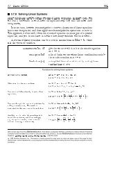
homogeneous systems of ODEs with constant coefficients.<br />
Linear Systems of ODEs<br />
Here is a system of two ODEs whose coefficient matrix has real and distinct eigenvalues.<br />
In[1]:= A = 884, -6
In[3]:= X@t_D = 8x@tD, y@tD
44 <strong>Differential</strong> <strong>Equation</strong> <strong>Solving</strong> with <strong>DSolve</strong><br />
This solves the system.<br />
In[12]:= sol = <strong>DSolve</strong>@system, 8x, y
In[16]:= sol = <strong>DSolve</strong>@8system@@1DD ã 0, system@@2DD ã 0
46 <strong>Differential</strong> <strong>Equation</strong> <strong>Solving</strong> with <strong>DSolve</strong><br />
In[21]:= X@t_D = 8x@tD, y@tD
In the following example, the algorithm finds one rational solution for x@tD and y@tD. (The equation<br />
for z@tD is uncoupled from the rest of the system.) Using the rational solution, <strong>DSolve</strong> is<br />
able to find the remaining exponential solution for x@tD and y@tD.<br />
In[31]:= system = 8x'@tD ã H2 * HH-9 + t + t^2L * x@tD + H-6 + t^2L * y@tDLL ê HH-2 + tL * tL,<br />
y'@tD ã H-3 * H-12 + 2 * t + t^2L * x@tD + H24 - 2 * t - 3 * t^2L * y@tDL ê HH-2 + tL * tL,<br />
z'@tD ã t * z@tD
48 <strong>Differential</strong> <strong>Equation</strong> <strong>Solving</strong> with <strong>DSolve</strong><br />
In[38]:= sol = <strong>DSolve</strong>@system, 8x, y
In[2]:= sol = <strong>DSolve</strong>@system, 8p, q, r, s
50 <strong>Differential</strong> <strong>Equation</strong> <strong>Solving</strong> with <strong>DSolve</strong><br />
The previous two examples demonstrate that the solutions to fairly simple systems are usually<br />
complicated expressions of the independent variable. In fact, the solution is often available only<br />
in implicit form and may thus contain InverseFunction objects or unevaluated Solve objects.<br />
Lie Symmetry Methods for <strong>Solving</strong> Nonlinear ODEs<br />
Around 1870, Marius Sophus Lie realized that many of the methods for solving differential<br />
equations could be unified using group theory. Lie symmetry methods are central to the mod-<br />
ern approach for studying nonlinear ODEs. They use the notion of symmetry to generate solutions<br />
in a systematic manner. Here is a brief introduction to Lie’s approach that provides some<br />
examples that are solved in this way by <strong>DSolve</strong>.<br />
A key notion in Lie’s method is that of an infinitesimal generator for a symmetry group. This<br />
concept is illustrated in the following example.<br />
Here is the well-known transformation for rotations in the x-y plane. This is a one-parameter<br />
group of transformations with parameter t.<br />
In[1]:= m = x * Cos@tD + y * Sin@tD;<br />
In[2]:= n = -x * Sin@tD + y * Cos@tD;<br />
For a fixed value of t, the point Hm, nL (in blue) can be obtained by rotating the line joining Hx, yL<br />
(in red) to the origin through an angle of t in the counterclockwise direction.<br />
In[3]:= Show@<br />
8Graphics@88Red, PointSize@0.04D, Point@83 * Cos@1 ê 4D, 3 * Sin@1 ê 4D
A rotation through t can be represented by the matrix<br />
Mt =<br />
cosHtL sinHtL<br />
-sinHtL cosHtL<br />
.<br />
This shows that the set of all rotations in the plane satisfies the properties for forming a group.<br />
In[3]:= M@t_D := 88Cos@tD, Sin@tD
52 <strong>Differential</strong> <strong>Equation</strong> <strong>Solving</strong> with <strong>DSolve</strong><br />
The rotation group arises in the study of symmetries of geometrical objects; it is an example of<br />
a symmetry group. The infinitesimal generator, a differential operator, is a convenient local<br />
representation for this symmetric group, which is a set of matrices.<br />
An expression that reduces to 0 under the action of the infinitesimal generator is called an<br />
invariant of the group.<br />
Here is an invariant for this group.<br />
In[12]:= invariant = x^2 + y^2;<br />
This states that the distance from the origin to Hx, yL, x 2 + y 2 , is preserved under rotation.<br />
In[13]:= v@invariantD<br />
Out[13]= 0<br />
In the following examples, these ideas are applied to differential equations.<br />
This is an example of a Riccati equation, from page 103 of [I99].<br />
In[14]:= Riccatiequation = y'@xD + y@xD^2 - 1 ê x^2 ã 0;<br />
The equation is invariant under the following scaling transformation.<br />
In[15]:= m = x * E^t;<br />
In[16]:= n = y * E^H-tL;<br />
The infinitesimal generator for this one-parameter group of transformations is found as before.<br />
In[17]:= Series@m, 8t, 0, 1
This shows that the expression for the Riccati equation in the Hx, y, pL coordinates is indeed<br />
invariant under prolongedv.<br />
In[21]:= Riccatiexpression = p + y^2 - H1 ê x^2L;<br />
In[22]:= prolongedv@RiccatiexpressionD ê. 8p Ø H1 ê x^2L - y^2< êê Together<br />
Out[22]= 0<br />
Depending on the order of the given equation, the knowledge of a symmetry (in the form of an<br />
infinitesimal generator) can be used in three ways.<br />
† If the order of the equation is 1, it gives an integrating factor for the ODE that makes the<br />
equation exact and hence solvable.<br />
† It gives a set of canonical coordinates in which the equation has a simple (integrable) form.<br />
† It reduces the problem of solving an ODE of order n to that of solving an ODE of order n - 1,<br />
which is typically a simpler problem.<br />
The <strong>DSolve</strong> function checks for certain standard types of symmetries in the given ODE and uses<br />
them to return a solution. Following are three examples of ODEs for which <strong>DSolve</strong> uses such a<br />
symmetry method.<br />
Here is a nonlinear first-order ODE (equation 1.120, page 315 of [K59]).<br />
In[23]:= FirstOrderODE = x * y'@xD ã y@xD * Hx * Log@x^2 ê y@xDD + 2L;<br />
This ODE has a symmetry with the following infinitesimal generator.<br />
In[24]:= v = H-2 * Exp@-xD * yL * D@Ò, yD &;<br />
The presence of this symmetry allows <strong>DSolve</strong> to calculate an integrating factor and return the<br />
solution.<br />
In[25]:= sol = <strong>DSolve</strong>@FirstOrderODE, y, xD<br />
Out[25]= 99y Ø FunctionA8x
54 <strong>Differential</strong> <strong>Equation</strong> <strong>Solving</strong> with <strong>DSolve</strong><br />
This equation is invariant under the following scaling transformation.<br />
In[28]:= m = x * E^t;<br />
In[29]:= n = y * E^t;<br />
The presence of this scaling symmetry allows <strong>DSolve</strong> to find new coordinates in which the<br />
independent variable is not explicitly present. Hence the problem is solved easily.<br />
In[30]:= sol = <strong>DSolve</strong>@SecondOrderODE, y, xD<br />
Solve::ifun : Inverse functions are being used by Solve, so some<br />
solutions may not be found; use Reduce for complete solution information. à<br />
Out[30]= ::y Ø FunctionB8x><br />
x<br />
This verifies the solution.<br />
In[31]:= SecondOrderODE ê. sol êê Simplify<br />
Out[31]= 8True<<br />
Finally, here is a system of two nonlinear first-order ODEs that can be solved by using a shift:<br />
u@xD Ø u@xD - x. After the shift, the system becomes autonomous (it does not depend explicitly on<br />
x) and hence it can be solved by reduction to a first-order ODE for v as a function of u. The<br />
Solve::ifun message can be ignored; it is generated while inverting the expression for<br />
Exp@vD to give an expression in terms of Log.<br />
In[32]:= Clear@u, vD<br />
In[33]:= NonlinearSystem = 8u'@xD ã Exp@v@xDD + 1, v'@xD ã u@xD - x
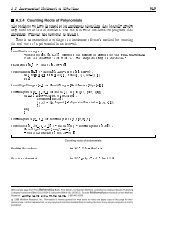
Partial <strong>Differential</strong> <strong>Equation</strong>s (PDEs)<br />
Introduction to Partial <strong>Differential</strong> <strong>Equation</strong>s (PDEs)<br />
A partial differential equation (PDE) is a relationship between an unknown function uHx1, x2, …, xnL<br />
and its derivatives with respect to the variables x1, x2, …, xn.<br />
Here is an example of a PDE.<br />
∂uHx, yL ∂uHx, yL<br />
In[1]:= equation1 = + x sinHxL;<br />
∂ x ∂ y<br />
PDEs occur naturally in applications; they model the rate of change of a physical quantity with<br />
respect to both space variables and time variables. At this stage of development, <strong>DSolve</strong> typi-<br />
cally only works with PDEs having two independent variables.<br />
The order of a PDE is the order of the highest derivative that occurs in it. The previous equation<br />
is a first-order PDE.<br />
A function uHx, yL is a solution to a given PDE if u and its derivatives satisfy the equation.<br />
Here is one solution to the previous equation.<br />
In[2]:= sol = u ê. <strong>DSolve</strong>@equation1, u, 8x, y
56 <strong>Differential</strong> <strong>Equation</strong> <strong>Solving</strong> with <strong>DSolve</strong><br />
name of equation general form classification<br />
transport equation<br />
Burgers’ equation<br />
∂u<br />
∂x<br />
∂u<br />
∂t<br />
∂u<br />
+ c 0 with c constant linear first-order PDE<br />
∂y<br />
∂u<br />
+ u 0 quasilinear first-order PDE<br />
∂x<br />
eikonal equation J ∂u<br />
∂x N2 + J ∂u<br />
∂y N2 1 nonlinear first-order PDE<br />
Laplace’s equation<br />
wave equation<br />
heat equation<br />
∂ 2 u<br />
∂x2 + ∂2u 0 elliptic linear second-order PDE<br />
2 ∂y<br />
∂ 2 u<br />
∂x2 = c2 ∂2u where c is the speed of light hyperbolic linear second-order<br />
2 ∂t<br />
PDE<br />
∂2u ∂u<br />
= k where k is the thermal<br />
2 ∂x ∂t<br />
diffusivity<br />
parabolic linear second-order PDE<br />
Recall that the general solutions to PDEs involve arbitrary functions rather than arbitrary con-<br />
stants. The reason for this can be seen from the following example.<br />
The partial derivative with respect to y does not appear in this example, so an arbitrary function<br />
C@1D@yD can be added to the solution, since the partial derivative of C@1D@yD with respect to x<br />
is 0.<br />
In[4]:= <strong>DSolve</strong>@D@u@x, yD, xD ã 1, u@x, yD, 8x, y
The PDE is said to be quasilinear if it can be expressed in the form<br />
∂uHx, yL<br />
∂uHx, yL<br />
aHx, y, uHx, yLL + bHx, y, uHx, yLL cHx, y, uHx, yLL.<br />
∂ x<br />
∂ y<br />
A PDE which is neither linear nor quasi-linear is said to nonlinear.<br />
For convenience, the symbols z, p, and q are used throughout this tutorial to denote the<br />
unknown function and its partial derivatives.<br />
∂uHx, yL ∂uHx, yL<br />
z = uHx, yL; p = ; q =<br />
∂ x<br />
∂ y<br />
Here is a linear homogeneous first-order PDE with constant coefficients.<br />
In[1]:= z := u@x, yD<br />
In[2]:= p := D@u@x, yD, xD<br />
In[3]:= q := D@u@x, yD, yD<br />
In[4]:= eqn = 2 * p + 3 * q + z ã 0;<br />
The equation is linear because the left-hand side is a linear polynomial in z, p, and q. Since<br />
there is no term free of z, p, or q, the PDE is also homogeneous.<br />
As mentioned earlier, the general solution contains an arbitrary function C@1D of the argument<br />
1<br />
H2 y - 3 xL.<br />
2<br />
In[5]:= sol = <strong>DSolve</strong>@eqn, u, 8x, y<br />
2<br />
This verifies that the solution is correct.<br />
In[6]:= eqn ê. sol@@1DD êê Simplify<br />
Out[6]= True<br />
Particular solutions of the homogeneous PDE are obtained by specifying the function C@1D.<br />
In[7]:= particularsolution = u@x, yD ê. sol@@1DD ê. C@1D@a_D Ø Sin@aD<br />
Out[7]= ‰ -xë2 SinB 1<br />
H-3 x + 2 yLF<br />
2<br />
<strong>Differential</strong> <strong>Equation</strong> <strong>Solving</strong> with <strong>DSolve</strong> 57
58 <strong>Differential</strong> <strong>Equation</strong> <strong>Solving</strong> with <strong>DSolve</strong><br />
Here is a plot of the surface for this particular solution.<br />
In[8]:= Plot3D@particularsolution, 8x, -2, 2
The first part of the solution, -10 + x + y, is the particular solution to the inhomogeneous PDE.<br />
The rest of the solution is the general solution to the homogenous equation.<br />
In[11]:= sol = u@x, yD ê. <strong>DSolve</strong>@eqn, u@x, yD, 8x, y
60 <strong>Differential</strong> <strong>Equation</strong> <strong>Solving</strong> with <strong>DSolve</strong><br />
Burgers’ equation is an important example of a quasi-linear PDE.<br />
∂uHx, yL ∂uHx, yL<br />
+ uHx, yL 0<br />
∂ x<br />
∂ y<br />
It can be written using the notation introduced earlier.<br />
In[20]:= Burgers<strong>Equation</strong> = p + z q ã 0;<br />
The term z q makes this equation quasi-linear.<br />
This solves the equation.<br />
In[21]:= sol = <strong>DSolve</strong>@Burgers<strong>Equation</strong>, u, 8x, y
The general solution to a first-order linear or quasi-linear PDE involves an arbitrary function. If<br />
the PDE is nonlinear, a very useful solution is given by the complete integral. This is a function<br />
of uHx, y, C@1D, C@2DL, where C@1D and C@2D are independent parameters and u satisfies the<br />
PDE for all values of HC@1D, C@2DL in an open subset of the plane. The complete integral can be<br />
used to find a general solution for the PDE as well as to solve initial value problems for it.<br />
Here is a simple nonlinear PDE.<br />
In[1]:= z := u@x, yD<br />
In[2]:= p := D@u@x, yD, xD<br />
In[3]:= q := D@u@x, yD, yD<br />
In[4]:= eqn = p * q ã 1;<br />
The complete integral depends on the parameters C@1D and C@2D. Since <strong>DSolve</strong> returns a<br />
general solution for linear and quasi-linear PDEs, a warning message appears before a complete<br />
integral is returned.<br />
In[5]:= sol = <strong>DSolve</strong>@eqn, u, 8x, y<br />
C@2D<br />
This verifies the solution.<br />
In[6]:= eqn ê. sol<br />
Out[6]= 8True<<br />
If the values of C@1D and C@2D are fixed, the previous solution represents a plane in three<br />
dimensions. Thus, the complete integral for this PDE is a two-parameter family of planes, each<br />
of which is a solution surface for the equation.<br />
Next, the envelope of a one-parameter family of surfaces is a surface that touches each mem-<br />
ber of the family. If the complete integral is restricted to a one-parameter family of planes, for<br />
example by setting C@2D = 5 C@1D, the envelope of this family is also a solution to the PDE<br />
called a general integral.<br />
<strong>Differential</strong> <strong>Equation</strong> <strong>Solving</strong> with <strong>DSolve</strong> 61
62 <strong>Differential</strong> <strong>Equation</strong> <strong>Solving</strong> with <strong>DSolve</strong><br />
This finds the envelope of the one-parameter family given by setting C@2D = 5 C@1D in the<br />
complete integral for the preceding PDE p * q == 1.<br />
In[7]:= oneparametersol = u@x, yD ã Hu@x, yD ê. sol@@1DD ê. C@2D Ø 5 * C@1DL<br />
x<br />
Out[7]= u@x, yD ã + C@1D + 5 y C@1D<br />
5 C@1D<br />
In[8]:= oneparameterenvelope =<br />
Eliminate@8oneparametersol, D@oneparametersol, C@1DD
Thus, the singular integral for this PDE is a plane parallel to the x-y plane.<br />
To summarize, the complete integral for a nonlinear PDE includes a rich variety of solutions.<br />
† Every member of the two-parameter family gives a particular solution to the PDE.<br />
† The envelope of any one-parameter family is a solution called a general integral of the PDE.<br />
† The envelope of the entire two-parameter family is a solution called the singular integral of<br />
the PDE.<br />
† The complete integral is not unique, but any other complete integral for the PDE can be<br />
obtained from it by the process of envelope formation.<br />
These remarkable properties account for the usefulness of the complete integral in geometrical<br />
optics, dynamics, and other areas of application. Following are various examples of nonlinear<br />
PDEs that show different kinds of complete integrals.<br />
Here is the complete integral for the eikonal equation.<br />
In[15]:= Eikonal = D@u@x, yD, xD^2 + D@u@x, yD, yD^2 == 1;<br />
In[16]:= sol = <strong>DSolve</strong>@Eikonal, u, 8x, y<br />
This complete integral is a two-parameter family of planes. This type of solution arises when-<br />
ever the PDE depends explicitly only on p and q, but not on u@x, yD, x, or y. For a fixed value of<br />
u@x, yD, it is a line in the plane at a distance of C@1D units from the origin that makes an angle of<br />
ArcCos@C@2DD with the x axis. This is the familiar picture of wave-front propagation from geo-<br />
metrical optics.<br />
This verifies the solution for the eikonal equation.<br />
In[17]:= Eikonal ê. sol<br />
Out[17]= 8True, True<<br />
This is an example of a Clairaut equation (z = p x + q y + f Hp, qL).<br />
In[18]:= Clairaut = z ã x * p + y * q + 2 p * q * Sqrt@1 - p^2D;<br />
<strong>Differential</strong> <strong>Equation</strong> <strong>Solving</strong> with <strong>DSolve</strong> 63
64 <strong>Differential</strong> <strong>Equation</strong> <strong>Solving</strong> with <strong>DSolve</strong><br />
Once again, the complete integral is a family of planes.<br />
In[19]:= sol = <strong>DSolve</strong>@Clairaut, u, 8x, y<br />
This verifies the solution.<br />
In[20]:= Clairaut ê. sol<br />
Out[20]= 8True<<br />
In the following equation, the variables can be separated; that is, the PDE can be written in the<br />
form f Hx, pL gHy, qL. Hence, the equation can be integrated easily.<br />
In[21]:= Separable = p^2 + a * q ã x + 3 y;<br />
In[22]:= sol = <strong>DSolve</strong>@Separable, u, 8x, y<br />
a<br />
This verifies the solution.<br />
In[23]:= Separable ê. sol êê Simplify<br />
Out[23]= 8True, True<<br />
In this example (equation 6.49, page 202 of [K74]), the independent variables x and y are not<br />
explicitly present.<br />
In[24]:= MissingIndependentVariables = a * p^2 + b * p * q ã c * z^2;<br />
In[25]:= sol = <strong>DSolve</strong>@MissingIndependentVariables, u, 8x, y
This verifies the solution.<br />
In[26]:= MissingIndependentVariables ê. sol êê Simplify<br />
Out[26]= 8True<<br />
Often a coordinate transformation can be used to cast a given PDE into one of the previous<br />
types. The expression for the complete integral will then have the same form as for the stan-<br />
dard types. Here are some examples of nonlinear PDEs for which <strong>DSolve</strong> applies a coordinate<br />
transformation to find the complete integral.<br />
This PDE (equation 6.47, page 201 of [K74]) can be reduced to the form f Hp, qL 0 using the<br />
transformation X = logHxL and Y = logHyL.<br />
In[27]:= <strong>DSolve</strong>@x * y * p * q ã 1, u@x, yD, 8x, y><br />
C@1D<br />
This PDE (equation 6.93, page 213 of [K74]) can be solved easily in a polar coordinate system,<br />
in which the variables are separable.<br />
In[28]:= <strong>DSolve</strong>@Hy * p - x * qL^2 + a * Hx * p + y * qL ã b, z, 8x, y>
66 <strong>Differential</strong> <strong>Equation</strong> <strong>Solving</strong> with <strong>DSolve</strong><br />
This verifies the solution.<br />
In[31]:= LegendreTransformable ê. sol êê Simplify<br />
Out[31]= 8True, True<<br />
It should be noted that there is no general practical algorithm for finding complete integrals,<br />
and that the answers are often available only in implicit form.<br />
The solution to this example (problem 2, page 66 of [S57]) is in implicit form.<br />
In[32]:= sol = <strong>DSolve</strong>@H1 + q^2L * z ã p * x, u, 8x, y
Here u = uHx, yL, and a, b, c, d, e, f , and g are functions of x and y only~they do not depend on u.<br />
If g = 0, the equation is said to be homogeneous.<br />
The first three terms containing the second derivatives are called the principal part of the PDE.<br />
They determine the nature of the general solution to the equation. In fact, the coefficients of<br />
the principal part can be used to classify the PDE as follows.<br />
The PDE is said to be elliptic if b 2 - 4 a c < 0. The Laplace equation has a = 1, b = 0, and c = 1 and is<br />
therefore an elliptic PDE.<br />
The PDE is said to be hyperbolic if b 2 - 4 a c > 0. The wave equation has a = 1, b = 0, and c = -1 and<br />
is therefore a hyperbolic PDE.<br />
The PDE is said to be parabolic if b 2 - 4 a c = 0. The heat equation has a = 1, b = 0, and c = 0 and is<br />
therefore a parabolic PDE.<br />
<strong>DSolve</strong> can find the general solution for a restricted type of homogeneous linear second-order<br />
PDEs; namely, equations of the form<br />
a ∂2 u<br />
∂ x2 + b ∂2 u<br />
∂ x ∂ y + c ∂2 u<br />
= 0.<br />
2 ∂ y<br />
Here a, b, and c are constants. Thus, <strong>DSolve</strong> assumes that the equation has constant coeffi-<br />
cients and a vanishing non-principal part.<br />
Following are some examples of the three basic types (elliptic, hyperbolic, and parabolic) and<br />
an explanation of their significance.<br />
Here is the general solution for Laplace’s equation, an elliptic PDE.<br />
In[1]:= Laplace<strong>Equation</strong> = D@u@x, yD, 8x, 2
68 <strong>Differential</strong> <strong>Equation</strong> <strong>Solving</strong> with <strong>DSolve</strong><br />
Here is another elliptic PDE.<br />
In[3]:= a = 3; b = 1; c = 5; b^2 - 4 a * c<br />
Out[3]= -59<br />
In[4]:= eqn = a * D@u@x, yD, 8x, 2
The solution can be verified as follows.<br />
In[12]:= eqn ê. sol êê Simplify<br />
Out[12]= 8True<<br />
Finally, here is an example of a parabolic PDE.<br />
In[13]:= a = 3; b = 30; c = 75; b^2 - 4 a * c<br />
Out[13]= 0<br />
In[14]:= eqn = a * D@u@x, yD, 8x, 2
70 <strong>Differential</strong> <strong>Equation</strong> <strong>Solving</strong> with <strong>DSolve</strong><br />
<strong>Differential</strong>-Algebraic <strong>Equation</strong>s (DAEs)<br />
Introduction to <strong>Differential</strong>-Algebraic <strong>Equation</strong>s<br />
(DAEs)<br />
The systems of equations that govern certain phenomena (in electrical circuits, chemical kinet-<br />
ics, etc.) contain a combination of differential equations and algebraic equations. The differential<br />
equations are responsible for the dynamical evolution of the system, while the algebraic<br />
equations serve to constrain the solutions to certain manifolds. It is therefore of some interest<br />
to study the solutions of such differential-algebraic equations (DAEs).<br />
Here is a simple example of a DAE. The first equation is an ODE for the function x@tD, while the<br />
second equation constrains the functions x@tD and y@tD to lie in a submanifold (a straight line) in<br />
8x, y< space.<br />
In[1]:= dae = 8x'@tD ã y@tD, x@tD + y@tD ã 1
It is important to realize that the initial values for a DAE must be prescribed carefully to guarantee<br />
a solution for the problem. This can be seen by considering the following system of<br />
equations.<br />
This gives<br />
8x1HtL + x2 £ HtL 0, x2HtL 0, x1H0L 1, x2H0L 0<<br />
x2HtL 0ï x2 £ HtL 0ï x1HtL 0.<br />
Hence the only solution is<br />
x1HtL 0 and x2HtL 0.<br />
But this solution is inconsistent with the initial condition x1H0L 1.<br />
<strong>DSolve</strong> can solve DAEs with constant coefficients; see "Examples of DAEs".<br />
Examples of DAEs<br />
This is a simple homogeneous DAE with constant coefficients.<br />
In[1]:= eqns = 8x'@tD - y@tD ã 0, x@tD + y@tD == 0
72 <strong>Differential</strong> <strong>Equation</strong> <strong>Solving</strong> with <strong>DSolve</strong><br />
The general solution is composed of the general solution to the corresponding homogeneous<br />
system and a particular solution to the inhomogeneous equation.<br />
In[5]:= sol = 8x@tD, y@tD< ê. <strong>DSolve</strong>@eqns, 8x@tD, y@tD<br />
2<br />
This solves an initial value problem for the previous equation.<br />
In[6]:= eqns = 8x'@tD - y@tD ã Sin@tD, x@tD + y@tD == 1, x@PiD == 1 ê 2
In this example, the algebraic constraint is present only implicitly: all three equations contain<br />
derivatives of the unknown functions.<br />
In[13]:= Clear@x1, x2, x3, t, eqnsD<br />
In[14]:= eqns = 8x2@tD + 2 x3@tD + x1 £ @tD - 2 x3 £ @tD == 0,<br />
-27 x1@tD - 22 x2@tD - 17 x3@tD - x1 £ @tD + 2 x3 £ @tD == 0,<br />
18 x1@tD + 14 x2@tD + 10 x3@tD + 2 x1 £ @tD + 3 x2 £ @tD + 2 x3 £ @tD == 0
74 <strong>Differential</strong> <strong>Equation</strong> <strong>Solving</strong> with <strong>DSolve</strong><br />
In[22]:= sol = <strong>DSolve</strong>@eqns, 8x, y
In[29]:=<br />
Out[29]= :9.156,<br />
Timing@sol = <strong>DSolve</strong>@HÒ1 == 0 &L êü eqns, 8p, q, r
76 <strong>Differential</strong> <strong>Equation</strong> <strong>Solving</strong> with <strong>DSolve</strong><br />
Initial and Boundary Value Problems<br />
Introduction to Initial and Boundary Value Problems<br />
<strong>DSolve</strong> can be used for finding the general solution to a differential equation or system of<br />
differential equations. The general solution gives information about the structure of the com-<br />
plete solution space for the problem. However, in practice, one is often interested only in particu-<br />
lar solutions that satisfy some conditions related to the area of application. These conditions are<br />
usually of two types.<br />
† The solution xHtL and/or its derivatives are required to have specific values at a single point,<br />
for example, xH0L 1 and x £ H0L 2. Such problems are traditionally called initial value problems<br />
(IVPs) because the system is assumed to start evolving from the fixed initial point (in<br />
this case, 0).<br />
† The solution xHtL is required to have specific values at a pair of points, for example, xH0L 3<br />
and xH1L 5. These problems are known as boundary value problems (BVPs) because the<br />
points 0 and 1 are regarded as boundary points (or edges) of the domain of interest in the<br />
application.<br />
The symbolic solution of both IVPs and BVPs requires knowledge of the general solution for the<br />
problem. The final step, in which the particular solution is obtained using the initial or boundary<br />
values, involves mostly algebraic operations, and is similar for IVPs and for BVPs.<br />
IVPs and BVPs for linear differential equations are solved rather easily since the final algebraic<br />
step involves the solution of linear equations. However, if the underlying equations are nonlinear,<br />
the solution could have several branches, or the arbitrary constants from the general<br />
solution could occur in different arguments of transcendental functions. As a result, it is not<br />
always possible to complete the final algebraic step for nonlinear problems. Finally, if the underlying<br />
equations have piecewise (that is, discontinuous) coefficients, an IVP naturally breaks up<br />
into simpler IVPs over the regions in which the coefficients are continuous.
Linear IVPs and BVPs<br />
To begin, consider an initial value problem for a linear first-order ODE.<br />
This is a linear first-order ODE.<br />
In[1]:= linearequation = y'@tD - 3 * t * y@tD ã 1;<br />
Notice that the general solution is a linear function of the arbitrary constant C@1D.<br />
In[2]:= generalsolution = <strong>DSolve</strong>@linearequation, y@tD, tD<br />
3 t<br />
Out[2]= ::y@tD Ø ‰<br />
2<br />
3 t<br />
2 C@1D + ‰<br />
2<br />
2<br />
p<br />
6<br />
ErfB<br />
3<br />
2<br />
tF>><br />
This finds a particular solution for the initial condition y@0D == 4.<br />
In[3]:= particularsolution = <strong>DSolve</strong>@8linearequation, y@0D ã 4<br />
This verifies that the solution satisfies both the equation and the initial condition.<br />
In[4]:= linearequation ê. particularsolution@@1DD<br />
Out[4]= True<br />
In[5]:= y@0D ê. particularsolution@@1DD<br />
Out[5]= 4<br />
Here is the solution to the same problem with the general initial condition y@0D == a.<br />
In[6]:= particularsolution = <strong>DSolve</strong>@8linearequation, y@0D ã a<br />
<strong>Differential</strong> <strong>Equation</strong> <strong>Solving</strong> with <strong>DSolve</strong> 77
78 <strong>Differential</strong> <strong>Equation</strong> <strong>Solving</strong> with <strong>DSolve</strong><br />
This plots several integral curves of the equation for different values of a. The plot shows that<br />
the solutions have an inflection point if the parameter a lies between -1 and 1, while a global<br />
maximum or minimum arises for other values of a.<br />
In[7]:= Plot@Evaluate@Table@y@tD ê. particularsolution@@1DD ê. a Ø i, 8i, -2, 2, 0.6
Here is a plot of the solution.<br />
In[14]:= Plot@x@tD ê. particularsolution, 8t, -1 ê 3, 2
80 <strong>Differential</strong> <strong>Equation</strong> <strong>Solving</strong> with <strong>DSolve</strong><br />
In[19]:= <strong>DSolve</strong>@8inhomogeneousequation, y@0D ã 1, y@1D ã 1 ê 2<br />
It should be noted that, in contrast to initial value problems, there are no general existence or<br />
uniqueness theorems when boundary values are prescribed, and there may be no solution in<br />
some cases.<br />
This problem has no solution because the term with C@2D in the general solution vanishes at<br />
both x 0 and x p. Hence there are two inconsistent conditions for the parameter C@1D and<br />
the solution is an empty set.<br />
In[20]:= <strong>DSolve</strong>@8inhomogeneousequation, y@0D ã 1, y@PiD ã 6
Finally, here is the solution of an IVP for a linear system of ODEs.<br />
In[25]:= Clear@x, y, z, tD<br />
In[26]:= linearsystem = 8x'@tD ã x@tD - 4 * y@tD + 1, y'@tD ã 4 * x@tD + y@tD, z'@tD ã z@tD
82 <strong>Differential</strong> <strong>Equation</strong> <strong>Solving</strong> with <strong>DSolve</strong><br />
In[31]:= ParametricPlot3D@Evaluate@8x@tD, y@tD, z@tD< ê. solD,<br />
8t, -7, -3
This solves the initial value problem for the logistic equation with symbolic parameters r and K.<br />
In[4]:= sol = <strong>DSolve</strong>@8Logistic<strong>Equation</strong>, y@0D ã a * K<br />
This verifies that the solution satisfies the equation and the initial condition.<br />
In[5]:= 8Logistic<strong>Equation</strong>, y@0D< ê. sol@@1DD êê Simplify<br />
Out[5]= 8True, a K<<br />
Here is a plot of the solution for different values of r and K.<br />
In[6]:= Plot@Evaluate@Table@y@tD ê. sol@@1DD ê. 8K Ø 4, a Ø i, r Ø H1 ê 3L
84 <strong>Differential</strong> <strong>Equation</strong> <strong>Solving</strong> with <strong>DSolve</strong><br />
Finally, here is a boundary value problem for a nonlinear second-order ODE. The solution is<br />
required to satisfy boundary conditions at 0 and infinity. The Solve::ifun message is generated<br />
while finding the general solution in terms of JacobiSN, the inverse of EllipticF. The<br />
<strong>DSolve</strong>::bvlim messages are given because the limit required for satisfying the condition<br />
y £ @InfinityD ã 0 cannot be calculated for either branch of the general solution. However, the<br />
solution for the boundary value problem is found using an alternative method to determine the<br />
values of the constants C@1D and C@2D in the general solution.<br />
In[10]:= generalsolution = <strong>DSolve</strong>@8y''@xD ê 2 ã y@xD^3 - y@xD, :y@xD Ø -Â -<br />
1<br />
1 + 1 - C@1D<br />
1 - 1 - C@1D<br />
JacobiSNB x 2 + x 2<br />
1 - 1 - C@1D<br />
F + Â -<br />
1<br />
1 + 1 - C@1D<br />
1 - 1 - C@1D<br />
x 2 + x 2<br />
1 - C@1D + 2 x C@2D + 2 x 1 - C@1D C@2D + C@2D 2 + 1 - C@1D C@2D 2 ,<br />
1 - C@1D JacobiSNB<br />
1 - C@1D + 2 x C@2D + 2 x 1 - C@1D C@2D + C@2D 2 + 1 - C@1D C@2D 2 ,<br />
1 - 1 - C@1D<br />
F>><br />
1 + 1 - C@1D<br />
In[11]:= sol =<br />
<strong>DSolve</strong>@8y''@xD ê 2 == y@xD^3 - y@xD, y@0D == 0, y'@InfinityD == 0, :y@xD Ø TanhB x 2 F>>
In[12]:= Plot@8y@xD ê. sol@@2DD, 1
86 <strong>Differential</strong> <strong>Equation</strong> <strong>Solving</strong> with <strong>DSolve</strong><br />
The solution can be plotted in the usual way. Note that the solution is continuous but not<br />
differentiable at x = 0.<br />
In[5]:= Plot@y@xD ê. sol, 8x, -3, 3 0 »» x < 0D<br />
Out[6]= 8True, True<<br />
Here is a piecewise ODE that has Max in its coefficients.<br />
In[7]:= sol = <strong>DSolve</strong>@ 8y'@xD + Max@x, 1D y@xD ã 0, y@0D ã 1><br />
True<br />
In[8]:= Plot@y@xD ê. sol, 8x, -3, 3
For this piecewise ODE, the expression for FinalSol is obtained by patching together<br />
SolFromMinusInfinityToTwo and SolFromTwoToInfinity. The boundary condition for<br />
the interval H-Infinity, 2D is simply y@0D = 1, while the initial condition for the interval<br />
@2, InfinityL is y@2D ‰ 2 (given by the final value for the solution over the first interval).<br />
In[9]:= FinalSol = <strong>DSolve</strong>@ 8y'@tD ã If@ t § 2, y@tD, -y@tD ê 2D , y@0D ã 1<br />
‰ 3- t<br />
2 True<br />
In[10]:= SolFromMinusInfinityToTwo = <strong>DSolve</strong>@8y'@tD ã y@tD, y@0D ã 1
88 <strong>Differential</strong> <strong>Equation</strong> <strong>Solving</strong> with <strong>DSolve</strong><br />
In[15]:= <strong>DSolve</strong>@eqn, y, xD<br />
Out[15]= ::y Ø FunctionB8x><br />
F +<br />
F Sin@1D Sin@xD +<br />
x §<br />
FN -1 <<br />
3 ‰ 2 AiryAiPrime@1D - 3 ‰ 2 x AiryAiPrime@1D + 3 ‰ 2 AiryBi@1D +<br />
3 ‰ 2 x AiryBi@1D - 3 ‰ 2 AiryBiPrime@1D + 3 ‰ 2 x AiryBiPrime@1DN GammaB 1<br />
3 F<br />
True
Working with <strong>DSolve</strong>~A User’s Guide<br />
Introduction to Working with <strong>DSolve</strong><br />
The aim of these tutorials is to provide a self-contained working guide for solving different types<br />
of problems with <strong>DSolve</strong>.<br />
The first step in using <strong>DSolve</strong> is to set up the problem correctly. The next step is to use <strong>DSolve</strong><br />
to get an expression for the solution. Once the solution has been found, it can be verified using<br />
symbolic or numerical techniques, or it can be plotted using a Mathematica function such as<br />
Plot, Plot3D, or ContourPlot. Plots often reveal information about the solution that might not<br />
be evident from its closed-form expression.<br />
If no boundary conditions are specified for a problem, the output from <strong>DSolve</strong> is some form of a<br />
general solution containing arbitrary parameters. The GeneratedParameters option can be<br />
used to label these arbitrary parameters.<br />
In many applications, differential equations contain symbolic parameters, such as the rate of<br />
growth in the logistic equation. A differential equation can also contain inexact quantities, such<br />
as machine numbers arising from previous calculations. Both symbolic parameters and inexact<br />
quantities are allowed by <strong>DSolve</strong>, but it is good to be aware of their presence and interpret the<br />
solution correctly.<br />
When <strong>DSolve</strong> makes any assumptions or encounters difficulty during a calculation, it issues a<br />
warning message outlining the problem. These messages can usually be ignored, but sometimes<br />
they point to serious limitations in the answer given for the problem.<br />
It is helpful to analyze the statement of the problem for possible ambiguities~in other words,<br />
to make sure that the problem is well posed~so that meaningful answers can be obtained from<br />
<strong>DSolve</strong>.<br />
<strong>Differential</strong> <strong>Equation</strong> <strong>Solving</strong> with <strong>DSolve</strong> 89
90 <strong>Differential</strong> <strong>Equation</strong> <strong>Solving</strong> with <strong>DSolve</strong><br />
Setting Up the Problem<br />
The first argument given to <strong>DSolve</strong> is the differential equation, the second argument is the<br />
unknown function, and the last argument identifies the independent variable.<br />
Here is the input for solving for a first-order linear ODE using <strong>DSolve</strong>. The variable sol identifies<br />
the solution for use in further work.<br />
In[1]:= sol = <strong>DSolve</strong>@y'@xD + 5 y@xD ã 1, y@xD, xD<br />
Out[1]= ::y@xD Ø 1<br />
5<br />
+ ‰ -5 x C@1D>><br />
The output of <strong>DSolve</strong> is a list of solutions for the differential equation. The extra list is required<br />
since some equations have multiple solutions. Here, since the equation is of order 1 and is<br />
linear, there is only one solution: y@xD Ø 1<br />
5 + ‰-5 x C@1D. The solution has an undetermined<br />
constant C@1D because no initial condition was specified. The solution can be extracted from the<br />
list of solutions using a part specification.<br />
This extracts the solution.<br />
In[2]:= m = sol@@1DD<br />
Out[2]= :y@xD Ø 1<br />
5<br />
+ ‰ -5 x C@1D><br />
This form of the solution is useful for finding y@xD itself, but not for finding derivatives of y@xD or<br />
the value of y@xD at a point.<br />
This shows the value of y@xD given by the solution.<br />
In[3]:= y@xD ê. m<br />
Out[3]=<br />
1<br />
5<br />
+ ‰ -5 x C@1D<br />
The solution does not apply to y £ @xD or y@1D because the solution is a rule for y@xD only.<br />
In[4]:= y'@xD ê. m<br />
Out[4]= y £ @xD<br />
In[5]:= y@1D ê. m<br />
Out[5]= y@1D<br />
If the solution will be used in further work, it is best to specify the unknown function using y<br />
rather than y@xD. This gives the solution using pure functions of the type Function@x, exprD.
If the solution will be used in further work, it is best to specify the unknown function using y<br />
rather than y@xD. This gives the solution using pure functions of the type Function@x, exprD.<br />
Here, the unknown function is specified as y. The solution is a pure function.<br />
In[6]:= sol = <strong>DSolve</strong>@y'@xD + 5 y@xD ã 1, y, xD<br />
Out[6]= ::y Ø FunctionB8x><br />
When the solution is in the form of pure functions, expressions can be found for derivatives of y<br />
and for the values of y at specific points.<br />
This gives expressions for y@xD, y £ @xD, and y@1D.<br />
In[7]:= m = sol@@1DD<br />
Out[7]= :y Ø FunctionB8x<br />
The solutions can be extracted using part specifications.<br />
In[12]:= y@xD ê. sol@@1DD<br />
Out[12]= - 2<br />
H11 + xL<br />
3<br />
3ë2 + C@1D<br />
<strong>Differential</strong> <strong>Equation</strong> <strong>Solving</strong> with <strong>DSolve</strong> 91
92 <strong>Differential</strong> <strong>Equation</strong> <strong>Solving</strong> with <strong>DSolve</strong><br />
In[13]:= y@xD ê. sol@@2DD<br />
Out[13]=<br />
2<br />
H11 + xL<br />
3<br />
3ë2 + C@1D<br />
This returns a list of both expressions.<br />
In[14]:= y@xD ê. sol<br />
Out[14]= :- 2<br />
H11 + xL<br />
3<br />
3ë2 + C@1D, 2<br />
H11 + xL<br />
3<br />
3ë2 + C@1D><br />
To solve a system of equations, the first argument to <strong>DSolve</strong> must be a list of the equations<br />
and the second argument must be a list of the unknown functions.<br />
Here is an example of a system of first-order linear equations with three unknowns. Because<br />
this system is linear, there is only one solution.<br />
In[15]:= sol = <strong>DSolve</strong>@<br />
8x'@tD ã y@tD + z@tD, y'@tD + z@tD - x@tD ã 0, z'@tD + y@tD ã x@tD
If only the initial value is specified, then the solution still contains an arbitrary constant.<br />
In[18]:= <strong>DSolve</strong>@8y''@xD + y@xD ã 5, y@0D ã 1
94 <strong>Differential</strong> <strong>Equation</strong> <strong>Solving</strong> with <strong>DSolve</strong><br />
The solutions to this equation are given as InverseFunction objects.<br />
In[23]:= sol = <strong>DSolve</strong>@Derivative@2D@yD@xD + y@xD * Derivative@1D@yD@xD^4 == 0, y, xD<br />
Solve::tdep :<br />
The equations appear to involve the variables to be solved for in an essentially non-algebraic way. à<br />
Solve::tdep :<br />
The equations appear to involve the variables to be solved for in an essentially non-algebraic way. à<br />
Out[23]= ::y Ø FunctionB8x, :y Ø<br />
FunctionB8x><br />
Each solution can be rewritten as an implicit equation by eliminating the InverseFunction<br />
object as follows.<br />
In[24]:= soly = y@xD ê. sol@@1DD<br />
Out[24]= InverseFunctionBC@1D LogBÒ1 + -2 C@1D + Ò1 2 F - 1<br />
Ò1<br />
2<br />
-2 C@1D + Ò1 2 &F@x + C@2DD<br />
In[25]:= implicitequation = H Head@solyD@@1DD@y@xDD == soly@@1DD L<br />
Out[25]= C@1D LogBy@xD + -2 C@1D + y@xD 2 F - 1<br />
y@xD<br />
2<br />
-2 C@1D + y@xD 2 ã x + C@2D<br />
Verification of the Solution<br />
The solution given by <strong>DSolve</strong> can be verified using various methods. The easiest method<br />
involves substituting the solution back into the equation. If the result is True, the solution is<br />
valid.<br />
In this simple example, the solution is verified by substitution. Note that the first argument to<br />
<strong>DSolve</strong> is assigned to eqn for convenience in later work.<br />
In[1]:= eqn = y'@xD ã x;<br />
In[2]:= sol = <strong>DSolve</strong>@eqn, y, xD<br />
Out[2]= ::y Ø FunctionB8x><br />
2<br />
In[3]:= eqn ê. sol<br />
Out[3]= 8True
In this example, the equation and an initial condition are verified by substitution.<br />
In[4]:= eqn = 8y'@xD ã x, y@0D ã 1<br />
In[6]:= eqn ê. sol<br />
Out[6]= 88True, True
96 <strong>Differential</strong> <strong>Equation</strong> <strong>Solving</strong> with <strong>DSolve</strong><br />
If the equation involves special functions, it may be necessary to use FullSimplify to verify<br />
the solution.<br />
Here is an example of this type involving Bessel’s functions.<br />
In[14]:= eqn = x * y''@xD + y'@xD - y@xD ã 1;<br />
In[15]:= sol = <strong>DSolve</strong>@eqn, y, xD<br />
Out[15]= ::y Ø FunctionB8x><br />
In[16]:= FullSimplify@eqn ê. solD<br />
Out[16]= 8True<<br />
If the solution is large or if Simplify and FullSimplify do not succeed in verifying the solu-<br />
tion, a numerical check can be made by using RandomReal or RandomComplex to generate<br />
values for all the variables and parameters in the problem. It is advisable in such cases to<br />
repeat the check with several sets of random values.<br />
Here is an example where numerical verification is useful.<br />
In[17]:= Clear@a, y, x, rD<br />
In[18]:= eqn = y''@xD - Ha * x^6 + x^2L * y@xD;<br />
In[19]:= sol = <strong>DSolve</strong>@eqn ã 0, y, xD<br />
Out[19]= ::y Ø FunctionB8x><br />
, 3 1<br />
, -<br />
4 2<br />
a x4F +<br />
In[20]:= Union@Flatten@Table@Chop@eqn ê. sol ê. 8x Ø RandomReal@D, a Ø RandomReal@D,<br />
C@1D Ø RandomReal@D, C@2D Ø RandomReal@D
This uses complex random values to verify the previous solution.<br />
In[22]:= r := RandomComplex@D<br />
In[23]:= Chop@N@eqn ê. sol ê. 8x Ø r, a Ø r , C@1D Ø r , C@2D Ø r
98 <strong>Differential</strong> <strong>Equation</strong> <strong>Solving</strong> with <strong>DSolve</strong><br />
Plotting the Solution<br />
A plot of the solution given by <strong>DSolve</strong> can give useful information about the nature of the<br />
solution, for instance, whether it is oscillatory in nature. It can also serve as a means of solu-<br />
tion verification if the shape of the graph is known from theory or from plotting the vector field<br />
associated with the differential equation. A few examples that use different Mathematica graph-<br />
ics functions follow.<br />
Here is the general solution to a linear first-order equation.<br />
In[1]:= sol = <strong>DSolve</strong>@y'@xD + x * y@xD ã Cos@x^2D, y, xD<br />
x2<br />
-<br />
Out[1]= ::y Ø FunctionB8x><br />
2<br />
The solution can be plotted for specific values of the constant C@1D using Plot. The use of<br />
Evaluate reduces the time taken by Plot and can also help in cases where the solution has<br />
discontinuities.<br />
In[2]:= Plot@Evaluate@y@xD ê. sol ê. 8C@1D Ø 1
This nonlinear equation has two solutions that can be plotted on the same graph.<br />
In[5]:= sol = <strong>DSolve</strong>@8y'@xD^2 ã x - x^3, y@0D ã 1<br />
In[6]:= Plot@Evaluate@y@xD ê. solD, 8x, 1 ê 100, 9 ê 10
100 <strong>Differential</strong> <strong>Equation</strong> <strong>Solving</strong> with <strong>DSolve</strong><br />
In[9]:= ContourPlot@expr, 8x, -0.4, -0.1
The ParametricPlot function can be used to trace the solution curve 8x@tD, y@tD< in the plane.<br />
In[12]:= ParametricPlot@Evaluate@8x@tD, y@tD< ê. solD, 8t, -1, 7
102 <strong>Differential</strong> <strong>Equation</strong> <strong>Solving</strong> with <strong>DSolve</strong><br />
Here is the general solution to a linear PDE.<br />
In[15]:= sol = <strong>DSolve</strong>@D@u@x, yD, xD + x^2 * D@u@x, yD, yD ã Exp@xD, u, 8x, y<br />
Here is a plot of the solution surface for a particular choice of the arbitrary function C@1D.<br />
In[16]:= Plot3D@Evaluate@u@x, yD ê. sol ê. 8C@1D@t_D Ø Sin@3 * tD
This shows the behavior of C.<br />
In[3]:= parameter = C@ÒD &;<br />
In[4]:= indexset = 81, 2, 3, 4
104 <strong>Differential</strong> <strong>Equation</strong> <strong>Solving</strong> with <strong>DSolve</strong><br />
In[11]:= <strong>DSolve</strong>@y''@xD + y@xD ã 1, y@xD, x, GeneratedParameters Ø Module@8C
It should be noted that the presence of symbolic parameters can lead to fairly complicated<br />
output.<br />
This is seen in the following example (equation 2.14, page 401 of [K59]).<br />
In[4]:= eqn = y''@xD - c * x^a * y@xD ;<br />
In[5]:= sol = <strong>DSolve</strong>@eqn ã 0, y, xD<br />
Out[5]= ::y Ø FunctionB8x><br />
2 + a 2 + a<br />
2+a<br />
2<br />
However, for some special values of the parameters, the solution might be significantly simpler.<br />
For these values of a and c, the solution is much more simple.<br />
In[6]:= sol1 = y@xD ê. sol@@1DD ê. 8a Ø 0, c Ø 4<<br />
Out[6]= C@1D Cosh@2 xD + 1<br />
 C@2D Sinh@2 xD<br />
2<br />
Occasionally, a solution is valid for most, but not all, values of the parameters.<br />
Since the input in this example is not valid at a = 0, the solution has the same limitation.<br />
In[7]:= sol = <strong>DSolve</strong>@8y'@xD ã x, y@0D ã 1 ê a<br />
2 a<br />
Of course, there is a simple remedy in this case: setting k = 1<br />
a .<br />
In[8]:= sol = <strong>DSolve</strong>@8y'@xD ã x, y@0D ã k<br />
In summary, the ability to solve differential equations with symbolic parameters is a powerful<br />
and essential feature of any symbolic solver such as <strong>DSolve</strong>. However, the following points<br />
should be noted.<br />
<strong>Differential</strong> <strong>Equation</strong> <strong>Solving</strong> with <strong>DSolve</strong> 105<br />
† The solution might be complicated, and such calculations often require significant time and<br />
memory.<br />
† The answer might not be valid for certain exceptional values of the parameters.<br />
† The solution might be easy to verify symbolically for some special values of the parameters,<br />
but in the general case a numerical verification method is preferable.
106 <strong>Differential</strong> <strong>Equation</strong> <strong>Solving</strong> with <strong>DSolve</strong><br />
†<br />
†<br />
The solution might be easy to verify symbolically for some special values of the parameters,<br />
but in the general case a numerical verification method is preferable.<br />
Numerical quantities in Mathematica can be of three types: infinite precision, machine preci-<br />
sion, or arbitrary precision. The first type of number is referred to as “exact”, while the remain-<br />
ing two types represent incomplete information and are therefore called “inexact”.<br />
Here is a simple example showing all three kinds of numbers.<br />
In[9]:= exactpi = Pi;<br />
In[10]:= Precision@exactpiD<br />
Out[10]= <br />
In[11]:= Hmachinepi = N@PiDL êê InputForm<br />
Out[11]//InputForm= 3.141592653589793<br />
In[12]:= Precision@machinepiD<br />
Out[12]= MachinePrecision<br />
In[13]:= highprecisionpi = N@Pi, 30D<br />
Out[13]= 3.14159265358979323846264338328<br />
In[14]:= Precision@highprecisionpiD<br />
Out[14]= 30.<br />
Since <strong>DSolve</strong> is a symbolic solver, the algorithms used by it are primarily based on the assump-<br />
tion of exact input. However, equations that contain inexact quantities are handled by <strong>DSolve</strong><br />
in the usual way.<br />
These equations contain the inexact number 3. and 3.`40, respectively.<br />
In[15]:= <strong>DSolve</strong>@x'@tD ã 3. x@tD, x, tD<br />
Out[15]= 99x Ø FunctionA8t
Here is a system of linear ODEs that all have exact coefficients. Note that even with a fairly<br />
small value of n, the calculation takes a long time to finish.<br />
In[17]:= n = 8;<br />
x0@t_D := 0;<br />
xn@t_D := 1;<br />
eqns = Table@8x i '@tD - H x i+1@tD - 2 x i@tD + x i-1@tDL, x i@0D - H1 ê nL
108 <strong>Differential</strong> <strong>Equation</strong> <strong>Solving</strong> with <strong>DSolve</strong><br />
Here the equation is converted to exact form before being solved.<br />
In[24]:= <strong>DSolve</strong>@Rationalize@8x'@tD ã 0.0001 * x@tD, x@0D ã 3.07><br />
<strong>DSolve</strong> returns a general solution for a problem if no initial or boundary conditions are specified.<br />
The general solution to this equation is returned.<br />
In[1]:= <strong>DSolve</strong>@y'@xD ã 1 - y@xD, y, xD<br />
Out[1]= 99y Ø FunctionA8x
Most problems that arise in practice are well-posed since they are derived from sound theoreti-<br />
cal principles. However, as a note of caution, the following are examples where <strong>DSolve</strong> might<br />
have difficulty finding a satisfactory solution to the problem.<br />
Here is the solution to a first-order ODE in which the right-hand side fails to satisfy the Lipschitz<br />
condition around 0.<br />
In[5]:= generalsol = <strong>DSolve</strong>@8y'@xD ã 1 ê y@xD<br />
The general solution has two branches.<br />
In[6]:= Plot@Evaluate@y@xD ê. generalsol ê. 8C@1D Ø 1
110 <strong>Differential</strong> <strong>Equation</strong> <strong>Solving</strong> with <strong>DSolve</strong><br />
In[10]:= sol = <strong>DSolve</strong>@8eqn, y@0D ã 1<br />
In[11]:= Table@eqn ê. sol ê. 8x Ø i
References<br />
[AB04] Abell, M. L. and J. P. Braselton. <strong>Differential</strong> <strong>Equation</strong>s with Mathematica, 3rd ed.<br />
Elsevier Academic Press, 2004.<br />
[A89] Abramov, S. A. "Rational Solutions of Linear <strong>Differential</strong> and Difference <strong>Equation</strong>s with<br />
Polynomial Coefficients." USSR Comput. Maths. Math. Phys. 29 (1989): 7|12.<br />
[A96] Abramov, S. A. "Symbolic Search Algorithms for Partial d'Alembertian Solutions of Linear<br />
<strong>Equation</strong>s." Programming and Computer Software 22, no. 1 (1996): 26.<br />
[AB01] Abramov, S. A. and M. Bronstein. "On Solutions of Linear Functional Systems." In Proc.<br />
ISSAC'01, 1|6, 2001.<br />
[AK91] Abramov, S. A. and K. Yu. Kvansenko. "Fast Algorithms to Search for the Rational<br />
Solutions of Linear <strong>Differential</strong> <strong>Equation</strong>s with Polynomial Coefficients." In Proc. ISSAC'91,<br />
267|270, 1991.<br />
[AP94] Abramov, S. A. and M. Petkovsek. "D'Alembertian Solutions of Linear <strong>Differential</strong> and<br />
Difference <strong>Equation</strong>s." In Proc. ISSAC'94, 169|174, 1994.<br />
[ABP95] Abramov, S. A., M. Bronstein, and M. Petkovsek. "On Polynomial Solutions of Linear<br />
Operator <strong>Equation</strong>s." In Proc. ISSAC'95, 290|296, 1995.<br />
[B93] Bocharov, A. "Symbolic Solvers for Nonlinear <strong>Differential</strong> <strong>Equation</strong>s." The Mathematica<br />
Journal 3, no. 2 (1993): 63|69.<br />
[BD97] Boyce, W. F. and R. C. DiPrima, Elementary <strong>Differential</strong> <strong>Equation</strong>s. John Wiley and<br />
Sons, 1997.<br />
[BM91] Boyer, C. B. and U. C. Merzbach, A History of Mathematics, 2nd ed. John Wiley, 1991.<br />
[B91] Bronstein, M. "The Risch <strong>Differential</strong> <strong>Equation</strong> on an Algebraic Curve." In Proc. ISSAC'91,<br />
241|246, 1991.<br />
[B92] Bronstein, M. "On Solutions of Linear Ordinary <strong>Differential</strong> <strong>Equation</strong>s in Their Coefficient<br />
Field." J. Symbolic Computation 13 (1992): 413|439.<br />
[B92a] Bronstein, M. "Integration and <strong>Differential</strong> <strong>Equation</strong>s in Computer Algebra."<br />
Programming and Computer Software 18, no.5 (1992): 201|217.<br />
[B92b] Bronstein, M. "Linear Ordinary <strong>Differential</strong> <strong>Equation</strong>s: Breaking Through the Order 2<br />
Barrier." In Proc. ISSAC'92, 42|48, 1992.<br />
<strong>Differential</strong> <strong>Equation</strong> <strong>Solving</strong> with <strong>DSolve</strong> 111
112 <strong>Differential</strong> <strong>Equation</strong> <strong>Solving</strong> with <strong>DSolve</strong><br />
[B92b] Bronstein, M. "Linear Ordinary <strong>Differential</strong> <strong>Equation</strong>s: Breaking through the Order 2<br />
Barrier." In Proc. ISSAC'92, 42|48, 1992.<br />
[C80] Campbell, S. L. Singular Systems of <strong>Differential</strong> <strong>Equation</strong>s I. Pitman, 1980.<br />
[C82] Campbell, S. L. Singular Systems of <strong>Differential</strong> <strong>Equation</strong>s II. Pitman, 1982.<br />
[CC04] Chan, L. and E. S. Cheb-Terrab. "Non-Liouvillian Solutions for Second Order Linear<br />
ODEs." In Proc. ISSAC'04, 80|86, 2004.<br />
[CDM97] Cheb-Terrab, E. S., L. G. S. Duarte, and L. A. C. P. da Mota. "Computer Algebra<br />
<strong>Solving</strong> of First Order ODEs Using Symmetry Methods." Comp. Phys. Comm. 101 (1997): 254.<br />
[CR99] Cheb-Terrab, E. S. and A. D. Roche. "Integrating Factors for Second Order ODEs." J.<br />
Symbolic Computation 27 (1999): 501.<br />
[CR00] Cheb-Terrab, E. S. and A. D. Roche. "Abel ODEs: Equivalence and Integrable Classes."<br />
Comp. Phys. Comm. 130 (2000): 204.<br />
[D58] Drazin, M. P. "Pseudo Inverses in Associative Rays and Semigroups" American<br />
Mathematical Monthly 65 (1958): 506|514.<br />
[F59] Forsyth, A. R. Theory of <strong>Differential</strong> <strong>Equation</strong>s. Dover, 1959.<br />
[I99] Ibragimov, N. H. Elementary Lie Group Analysis and Ordinary <strong>Differential</strong> <strong>Equation</strong>s. John<br />
Wiley & Sons, 1999.<br />
[I44] Ince, E. L. Ordinary <strong>Differential</strong> <strong>Equation</strong>s. Dover, 1944.<br />
[K59] Kamke, E. <strong>Differential</strong>gleichungen: Losungsmethoden und Losungen. Akademische<br />
Verlagsgesellschaft, 1959.<br />
[K74] Kamke, E. <strong>Differential</strong>gleichungen Losungsmethoden und Losungen, Bd. II: Partielle<br />
differentialgleichungen. Chelsea Publishing Co., 1974.<br />
[K00] Kevorkian, J. Partial <strong>Differential</strong> <strong>Equation</strong>s: Analytical Solution Techniques. Springer-<br />
Verlag, 2000.<br />
[K72] Kline, M. Mathematical Thought from Ancient to Modern Times, Vol. 2. Oxford University<br />
Press, 1972.<br />
[K86] Kovacic, J. J. "An Algorithm for <strong>Solving</strong> Second Order Linear Homogeneous <strong>Differential</strong><br />
<strong>Equation</strong>s." J. Symbolic Computation 2 (1986): 3|43.<br />
[L01] Kovacic, J. J. "An Algorithm for <strong>Solving</strong> Second Order Linear Homogeneous <strong>Differential</strong><br />
<strong>Equation</strong>s." Lecture, City College of New York, 2001.
[L01] Kovacic, J. J. "An Algorithm for <strong>Solving</strong> Second Order Linear Homogeneous <strong>Differential</strong><br />
<strong>Equation</strong>s." Lecture, City College of New York, 2001.<br />
[KPS03] Kythe, P. K., P. Puri, and M. R. Schäferkotter, Partial <strong>Differential</strong> <strong>Equation</strong>s and<br />
Boundary Value Problems with Mathematica, 2nd ed. Chapman and Hall/CRC, 2003.<br />
[L65] Lebedev, N. N. Special Functions and Their Applications. Prentice-Hall, 1965.<br />
[M00] Meyer, C. D. Matrix Analysis and Applied Linear Algebra. SIAM, 2000.<br />
[M60] Murphy, G. M. Ordinary <strong>Differential</strong> <strong>Equation</strong>s and Their Solutions. Van Nostrand, 1960.<br />
[M47] McLachlan, N. W. Theory and Application of Mathieu Functions. Oxford University Press,<br />
1947.<br />
[O95] Olver, P. J. Equivalence, Invariants and Symmetry. Cambridge University Press, 1995.<br />
[PZ95] Polynanin, A. D. and V. F. Zaitsev, Handbook of Exact Solutions for Ordinary <strong>Differential</strong><br />
<strong>Equation</strong>s. CRC Press, 1995.<br />
[S81] Saunders, B. D. "An Implementation of Kovacic's Algorithm for <strong>Solving</strong> Second Order<br />
Linear Homogeneous <strong>Differential</strong> <strong>Equation</strong>s." In Proc. SYMSAC'81 (P. Wang, ed.), 105, 1981.<br />
[S85] Schlesinger, L. Handbuch der Theorie der Linearen <strong>Differential</strong>gleichungen. Teubner,<br />
1985.<br />
[SS98] Shirvani, M. and J. W.-H. So. "Solutions of Linear <strong>Differential</strong> Algebraic <strong>Equation</strong>s."<br />
SIAM Review 40, no. 2 (1998): 344|346.<br />
[S57] Sneddon, I. Elements of Partial <strong>Differential</strong> <strong>Equation</strong>s. McGraw-Hill, 1957.<br />
[T05] Trott, M. The Mathematica GuideBook for Symbolics. Springer-Verlag, 2005.<br />
[UW96] Ulmer, F. and J-A. Weil. "Note on Kovacic's Algorithm." J. Symbolic Computation 22<br />
(1996): 179|200.<br />
[WW27] Whittaker, E. T. and G. N. Watson. A Course of Modern Analysis, 4th ed. Cambridge<br />
University Press, 1927.<br />
[W02] <strong>Wolfram</strong>, S. A New Kind of Science. <strong>Wolfram</strong> Media, Inc., 2002.<br />
[W04] <strong>Wolfram</strong>, S. The Mathematica Book, 5th ed. <strong>Wolfram</strong> Media, Inc., 2004.<br />
[Z89] Zwillinger, D. Handbook of <strong>Differential</strong> <strong>Equation</strong>s. Academic Press, 1989<br />
<strong>Differential</strong> <strong>Equation</strong> <strong>Solving</strong> with <strong>DSolve</strong> 113