Advanced Numerical Differential Equation Solving in Mathematica
Advanced Numerical Differential Equation Solving in Mathematica
Advanced Numerical Differential Equation Solving in Mathematica

Create successful ePaper yourself
Turn your PDF publications into a flip-book with our unique Google optimized e-Paper software.
Wolfram <strong>Mathematica</strong> ® Tutorial Collection<br />
ADVANCED NUMERICAL DIFFERENTIAL<br />
EQUATION SOLVING IN MATHEMATICA
For use with Wolfram <strong>Mathematica</strong> ® 7.0 and later.<br />
For the latest updates and corrections to this manual:<br />
visit reference.wolfram.com<br />
For <strong>in</strong>formation on additional copies of this documentation:<br />
visit the Customer Service website at www.wolfram.com/services/customerservice<br />
or email Customer Service at <strong>in</strong>fo@wolfram.com<br />
Comments on this manual are welcomed at:<br />
comments@wolfram.com<br />
Content authored by:<br />
Mark Sofroniou and Rob Knapp<br />
Pr<strong>in</strong>ted <strong>in</strong> the United States of America.<br />
15 14 13 12 11 10 9 8 7 6 5 4 3 2<br />
©2008 Wolfram Research, Inc.<br />
All rights reserved. No part of this document may be reproduced or transmitted, <strong>in</strong> any form or by any means,<br />
electronic, mechanical, photocopy<strong>in</strong>g, record<strong>in</strong>g or otherwise, without the prior written permission of the copyright<br />
holder.<br />
Wolfram Research is the holder of the copyright to the Wolfram <strong>Mathematica</strong> software system ("Software") described<br />
<strong>in</strong> this document, <strong>in</strong>clud<strong>in</strong>g without limitation such aspects of the system as its code, structure, sequence,<br />
organization, “look and feel,” programm<strong>in</strong>g language, and compilation of command names. Use of the Software unless<br />
pursuant to the terms of a license granted by Wolfram Research or as otherwise authorized by law is an <strong>in</strong>fr<strong>in</strong>gement<br />
of the copyright.<br />
Wolfram Research, Inc. and Wolfram Media, Inc. ("Wolfram") make no representations, express,<br />
statutory, or implied, with respect to the Software (or any aspect thereof), <strong>in</strong>clud<strong>in</strong>g, without limitation,<br />
any implied warranties of merchantability, <strong>in</strong>teroperability, or fitness for a particular purpose, all of<br />
which are expressly disclaimed. Wolfram does not warrant that the functions of the Software will meet<br />
your requirements or that the operation of the Software will be un<strong>in</strong>terrupted or error free. As such,<br />
Wolfram does not recommend the use of the software described <strong>in</strong> this document for applications <strong>in</strong><br />
which errors or omissions could threaten life, <strong>in</strong>jury or significant loss.<br />
<strong>Mathematica</strong>, MathL<strong>in</strong>k, and MathSource are registered trademarks of Wolfram Research, Inc. J/L<strong>in</strong>k, MathLM,<br />
.NET/L<strong>in</strong>k, and web<strong>Mathematica</strong> are trademarks of Wolfram Research, Inc. W<strong>in</strong>dows is a registered trademark of<br />
Microsoft Corporation <strong>in</strong> the United States and other countries. Mac<strong>in</strong>tosh is a registered trademark of Apple<br />
Computer, Inc. All other trademarks used here<strong>in</strong> are the property of their respective owners. <strong>Mathematica</strong> is not<br />
associated with <strong>Mathematica</strong> Policy Research, Inc.
Contents<br />
Introduction . . . . . . . . . . . . . . . . . . . . . . . . . . . . . . . . . . . . . . . . . . . . . . . . . . . . . . . . . . . . . . . . . . . . . . . . 1<br />
Overview . . . . . . . . . . . . . . . . . . . . . . . . . . . . . . . . . . . . . . . . . . . . . . . . . . . . . . . . . . . . . . . . . . . . . . . 1<br />
The Design of the NDSolve Framework . . . . . . . . . . . . . . . . . . . . . . . . . . . . . . . . . . . . . . . . . . 11<br />
ODE Integration Methods . . . . . . . . . . . . . . . . . . . . . . . . . . . . . . . . . . . . . . . . . . . . . . . . . . . . . . . . . 17<br />
Methods . . . . . . . . . . . . . . . . . . . . . . . . . . . . . . . . . . . . . . . . . . . . . . . . . . . . . . . . . . . . . . . . . . . . . . . . 17<br />
Controller Methods . . . . . . . . . . . . . . . . . . . . . . . . . . . . . . . . . . . . . . . . . . . . . . . . . . . . . . . . . . . . . 66<br />
Extensions . . . . . . . . . . . . . . . . . . . . . . . . . . . . . . . . . . . . . . . . . . . . . . . . . . . . . . . . . . . . . . . . . . . . . . 162<br />
Partial <strong>Differential</strong> <strong>Equation</strong>s . . . . . . . . . . . . . . . . . . . . . . . . . . . . . . . . . . . . . . . . . . . . . . . . . . . . . 174<br />
The <strong>Numerical</strong> Method of L<strong>in</strong>es . . . . . . . . . . . . . . . . . . . . . . . . . . . . . . . . . . . . . . . . . . . . . . . . . 174<br />
Boundary Value Problems . . . . . . . . . . . . . . . . . . . . . . . . . . . . . . . . . . . . . . . . . . . . . . . . . . . . . . . . . 243<br />
Shoot<strong>in</strong>g Method . . . . . . . . . . . . . . . . . . . . . . . . . . . . . . . . . . . . . . . . . . . . . . . . . . . . . . . . . . . . . . . 243<br />
Chas<strong>in</strong>g Method . . . . . . . . . . . . . . . . . . . . . . . . . . . . . . . . . . . . . . . . . . . . . . . . . . . . . . . . . . . . . . . . 248<br />
Boundary Value Problems with Parameters . . . . . . . . . . . . . . . . . . . . . . . . . . . . . . . . . . . . . 255<br />
<strong>Differential</strong>-Algebraic <strong>Equation</strong>s . . . . . . . . . . . . . . . . . . . . . . . . . . . . . . . . . . . . . . . . . . . . . . . . . . 256<br />
Introduction . . . . . . . . . . . . . . . . . . . . . . . . . . . . . . . . . . . . . . . . . . . . . . . . . . . . . . . . . . . . . . . . . . . . 256<br />
IDA Method . . . . . . . . . . . . . . . . . . . . . . . . . . . . . . . . . . . . . . . . . . . . . . . . . . . . . . . . . . . . . . . . . . . . . 264<br />
Delay <strong>Differential</strong> <strong>Equation</strong>s . . . . . . . . . . . . . . . . . . . . . . . . . . . . . . . . . . . . . . . . . . . . . . . . . . . . . . 274<br />
Comparison and Contrast with ODEs . . . . . . . . . . . . . . . . . . . . . . . . . . . . . . . . . . . . . . . . . . . . 275<br />
Propagation and Smooth<strong>in</strong>g of Discont<strong>in</strong>uities . . . . . . . . . . . . . . . . . . . . . . . . . . . . . . . . . . 280<br />
Stor<strong>in</strong>g History Data . . . . . . . . . . . . . . . . . . . . . . . . . . . . . . . . . . . . . . . . . . . . . . . . . . . . . . . . . . . . 284<br />
The Method of Steps . . . . . . . . . . . . . . . . . . . . . . . . . . . . . . . . . . . . . . . . . . . . . . . . . . . . . . . . . . . . 285<br />
Examples . . . . . . . . . . . . . . . . . . . . . . . . . . . . . . . . . . . . . . . . . . . . . . . . . . . . . . . . . . . . . . . . . . . . . . . 290<br />
Norms <strong>in</strong> NDSolve . . . . . . . . . . . . . . . . . . . . . . . . . . . . . . . . . . . . . . . . . . . . . . . . . . . . . . . . . . . . . . . . . . 294<br />
ScaledVectorNorm . . . . . . . . . . . . . . . . . . . . . . . . . . . . . . . . . . . . . . . . . . . . . . . . . . . . . . . . . . . . . . 296<br />
Stiffness Detection . . . . . . . . . . . . . . . . . . . . . . . . . . . . . . . . . . . . . . . . . . . . . . . . . . . . . . . . . . . . . . . . . 298<br />
Overview . . . . . . . . . . . . . . . . . . . . . . . . . . . . . . . . . . . . . . . . . . . . . . . . . . . . . . . . . . . . . . . . . . . . . . . 298<br />
Introduction . . . . . . . . . . . . . . . . . . . . . . . . . . . . . . . . . . . . . . . . . . . . . . . . . . . . . . . . . . . . . . . . . . . . 299<br />
L<strong>in</strong>ear Stability . . . . . . . . . . . . . . . . . . . . . . . . . . . . . . . . . . . . . . . . . . . . . . . . . . . . . . . . . . . . . . . . . 301<br />
"StiffnessTest" Method Option . . . . . . . . . . . . . . . . . . . . . . . . . . . . . . . . . . . . . . . . . . . . . . . . . . 304<br />
"NonstiffTest" Method Option . . . . . . . . . . . . . . . . . . . . . . . . . . . . . . . . . . . . . . . . . . . . . . . . . . . 305<br />
Examples . . . . . . . . . . . . . . . . . . . . . . . . . . . . . . . . . . . . . . . . . . . . . . . . . . . . . . . . . . . . . . . . . . . . . . . 315<br />
Option Summary . . . . . . . . . . . . . . . . . . . . . . . . . . . . . . . . . . . . . . . . . . . . . . . . . . . . . . . . . . . . . . . . 323<br />
Structured Systems . . . . . . . . . . . . . . . . . . . . . . . . . . . . . . . . . . . . . . . . . . . . . . . . . . . . . . . . . . . . . . . . 324
Structured Systems . . . . . . . . . . . . . . . . . . . . . . . . . . . . . . . . . . . . . . . . . . . . . . . . . . . . . . . . . . . . . . . . 324<br />
<strong>Numerical</strong> Methods for <strong>Solv<strong>in</strong>g</strong> the Lotka|Volterra <strong>Equation</strong>s . . . . . . . . . . . . . . . . . . . . 324<br />
Rigid Body Solvers . . . . . . . . . . . . . . . . . . . . . . . . . . . . . . . . . . . . . . . . . . . . . . . . . . . . . . . . . . . . . . 329<br />
Components and Data Structures . . . . . . . . . . . . . . . . . . . . . . . . . . . . . . . . . . . . . . . . . . . . . . . . . 339<br />
Introduction . . . . . . . . . . . . . . . . . . . . . . . . . . . . . . . . . . . . . . . . . . . . . . . . . . . . . . . . . . . . . . . . . . . . 339<br />
Example . . . . . . . . . . . . . . . . . . . . . . . . . . . . . . . . . . . . . . . . . . . . . . . . . . . . . . . . . . . . . . . . . . . . . . . . 340<br />
Creat<strong>in</strong>g NDSolve`StateData Objects . . . . . . . . . . . . . . . . . . . . . . . . . . . . . . . . . . . . . . . . . . . 341<br />
Iterat<strong>in</strong>g Solutions . . . . . . . . . . . . . . . . . . . . . . . . . . . . . . . . . . . . . . . . . . . . . . . . . . . . . . . . . . . . . 343<br />
Gett<strong>in</strong>g Solution Functions . . . . . . . . . . . . . . . . . . . . . . . . . . . . . . . . . . . . . . . . . . . . . . . . . . . . . . 344<br />
NDSolve`StateData methods . . . . . . . . . . . . . . . . . . . . . . . . . . . . . . . . . . . . . . . . . . . . . . . . . . . 348<br />
<strong>Differential</strong><strong>Equation</strong>s Utility Packages . . . . . . . . . . . . . . . . . . . . . . . . . . . . . . . . . . . . . . . . . . . 351<br />
Interpolat<strong>in</strong>gFunctionAnatomy . . . . . . . . . . . . . . . . . . . . . . . . . . . . . . . . . . . . . . . . . . . . . . . . . 351<br />
NDSolveUtilities . . . . . . . . . . . . . . . . . . . . . . . . . . . . . . . . . . . . . . . . . . . . . . . . . . . . . . . . . . . . . . . . 356<br />
References . . . . . . . . . . . . . . . . . . . . . . . . . . . . . . . . . . . . . . . . . . . . . . . . . . . . . . . . . . . . . . . . . . . . . . . . . 358
Introduction to <strong>Advanced</strong> <strong>Numerical</strong><br />
<strong>Differential</strong> <strong>Equation</strong> <strong>Solv<strong>in</strong>g</strong> <strong>in</strong><br />
<strong>Mathematica</strong><br />
Overview<br />
The <strong>Mathematica</strong> function NDSolve is a general numerical differential equation solver. It can<br />
handle a wide range of ord<strong>in</strong>ary differential equations (ODEs) as well as some partial differential<br />
equations (PDEs). In a system of ord<strong>in</strong>ary differential equations there can be any number of<br />
unknown functions xi, but all of these functions must depend on a s<strong>in</strong>gle “<strong>in</strong>dependent variable”<br />
t, which is the same for each function. Partial differential equations <strong>in</strong>volve two or more <strong>in</strong>depen-<br />
dent variables. NDSolve can also solve some differential-algebraic equations (DAEs), which are<br />
typically a mix of differential and algebraic equations.<br />
NDSolve@8eqn 1 ,eqn 2 ,…
2 <strong>Advanced</strong> <strong>Numerical</strong> <strong>Differential</strong> <strong>Equation</strong> <strong>Solv<strong>in</strong>g</strong> <strong>in</strong> <strong>Mathematica</strong><br />
can solve nearly all <strong>in</strong>itial value prob-<br />
lems that can symbolically be put <strong>in</strong> normal form (i.e. are solvable for the highest derivative<br />
order), but only l<strong>in</strong>ear boundary value problems.<br />
This f<strong>in</strong>ds a solution for x with t <strong>in</strong> the range 0 to 2, us<strong>in</strong>g an <strong>in</strong>itial condition for x at t ã 1.<br />
In[1]:= NDSolve@8x‘@tD == x@tD, x@1D == 3
Here is a simple boundary value problem.<br />
In[4]:= NDSolve@8y‘‘@xD + x y@xD == 0, y@0D == 1, y@1D == -1
4 <strong>Advanced</strong> <strong>Numerical</strong> <strong>Differential</strong> <strong>Equation</strong> <strong>Solv<strong>in</strong>g</strong> <strong>in</strong> <strong>Mathematica</strong><br />
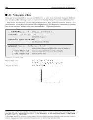
This shows the real part of the solutions that NDSolve was able to f<strong>in</strong>d. (The upper two solutions<br />
are strictly real.)<br />
In[8]:= Plot@Evaluate@Part@Re@y@xD ê. %D, 81, 2, 4
This shows a plot of the solutions.<br />
In[10]:= Plot@Evaluate@8x@tD, y@tD< ê. %D, 8t, 0, 1.66
6 <strong>Advanced</strong> <strong>Numerical</strong> <strong>Differential</strong> <strong>Equation</strong> <strong>Solv<strong>in</strong>g</strong> <strong>in</strong> <strong>Mathematica</strong><br />
This actually computes an approximate solution of the heat equation for a rod with constant<br />
temperatures at either end of the rod. (For more accurate solutions, you can <strong>in</strong>crease n.)<br />
The result is an approximate solution to the heat equation for a 1-dimensional rod of length 1<br />
with constant temperature ma<strong>in</strong>ta<strong>in</strong>ed at either end. This shows the solutions considered as<br />
spatial values as a function of time.<br />
In[17]:= ListPlot3D@Table@vars ê. First@%D, 8t, 0, .25, .025
NDSolve@8eqn 1 ,eqn 2 ,…
8 <strong>Advanced</strong> <strong>Numerical</strong> <strong>Differential</strong> <strong>Equation</strong> <strong>Solv<strong>in</strong>g</strong> <strong>in</strong> <strong>Mathematica</strong><br />
This f<strong>in</strong>ds a numerical solution to a generalization of the nonl<strong>in</strong>ear s<strong>in</strong>e-Gordon equation to two<br />
spatial dimensions with periodic boundary conditions.<br />
In[22]:= NDSolveA9D@u@t, x, yD, t, tD ã<br />
D@u@t, x, yD, x, xD + D@u@t, x, yD, y, yD - S<strong>in</strong>@u@t, x, yDD,<br />
u@0, x, yD ã ExpA-Ix 2 + y 2 ME, Derivative@1, 0, 0D@uD@0, x, yD ã 0,<br />
u@t, -5, yD ã u@t, 5, yD ã 0, u@t, x, -5D ã u@t, x, 5D ã 0=,<br />
u, 8t, 0, 3
NDSolve uses the sett<strong>in</strong>g you give for Work<strong>in</strong>gPrecision to determ<strong>in</strong>e the precision to use <strong>in</strong><br />
its <strong>in</strong>ternal computations. If you specify large values for AccuracyGoal or PrecisionGoal, then<br />
you typically need to give a somewhat larger value for Work<strong>in</strong>gPrecision. With the default<br />
sett<strong>in</strong>g of Automatic, both AccuracyGoal and PrecisionGoal are equal to half of the sett<strong>in</strong>g<br />
for Work<strong>in</strong>gPrecision.<br />
NDSolve uses error estimates for determ<strong>in</strong><strong>in</strong>g whether it is meet<strong>in</strong>g the specified tolerances.<br />
When work<strong>in</strong>g with systems of equations, it uses the sett<strong>in</strong>g of the option NormFunction -> f to<br />
comb<strong>in</strong>e errors <strong>in</strong> different components. The norm is scaled <strong>in</strong> terms of the tolerances, given so<br />
that NDSolve tries to take steps such that<br />
f<br />
err1<br />
err2<br />
,<br />
, … § 1<br />
tolr Abs@x1D + tola tolr Abs@x2D + tola<br />
where erri is the i th component of the error and xi is the i th component of the current solution.<br />
This generates a high-precision solution to a differential equation.<br />
In[24]:= NDSolve@8x‘‘‘@tD == x@tD, x@0D == 1, x‘@0D == x‘‘@0D == 0 20, Work<strong>in</strong>gPrecision -> 25D<br />
Out[24]= 88x Ø Interpolat<strong>in</strong>gFunction@880, 1.000000000000000000000000
10 <strong>Advanced</strong> <strong>Numerical</strong> <strong>Differential</strong> <strong>Equation</strong> <strong>Solv<strong>in</strong>g</strong> <strong>in</strong> <strong>Mathematica</strong><br />
NDSolve stops after tak<strong>in</strong>g 10,000 steps.<br />
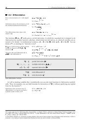
In[26]:= NDSolve@8y‘@xD == 1 ê x^2, y@-1D == 1 Automatic, NDSolve will<br />
choose a method which should be appropriate for the differential equations. For example, if the<br />
equations have stiffness, implicit methods will be used as needed, or if the equations make a<br />
DAE, a special DAE method will be used. In general, it is not possible to determ<strong>in</strong>e the nature of<br />
solutions to differential equations without actually solv<strong>in</strong>g them: thus, the default Automatic<br />
methods are good for solv<strong>in</strong>g as wide variety of problems, but the one chosen may not be the<br />
best one available for your particular problem. Also, you may want to choose methods, such as<br />
symplectic <strong>in</strong>tegrators, which preserve certa<strong>in</strong> properties of the solution.<br />
Choos<strong>in</strong>g an appropriate method for a particular system can be quite difficult. To complicate it<br />
further, many methods have their own sett<strong>in</strong>gs, which can greatly affect solution efficiency and<br />
accuracy. Much of this documentation consists of descriptions of methods to give you an idea of<br />
when they should be used and how to adjust them to solve particular problems. Furthermore,<br />
NDSolve has a mechanism that allows you to def<strong>in</strong>e your own methods and still have the<br />
equations and results processed by NDSolve just as for the built-<strong>in</strong> methods.
When NDSolve computes a solution, there are typically three phases. First, the equations are<br />
processed, usually <strong>in</strong>to a function that represents the right-hand side of the equations <strong>in</strong> normal<br />
form. Next, the function is used to iterate the solution from the <strong>in</strong>itial conditions. F<strong>in</strong>ally, data<br />
saved dur<strong>in</strong>g the iteration procedure is processed <strong>in</strong>to one or more Interpolat<strong>in</strong>gFunction<br />
objects. Us<strong>in</strong>g functions <strong>in</strong> the NDSolve` context, you can run these steps separately and, more<br />
importantly, have more control over the iteration process. The steps are tied by an<br />
NDSolve`StateData object, which keeps all of the data necessary for solv<strong>in</strong>g the differential<br />
equations.<br />
The Design of the NDSolve Framework<br />
Features<br />
Support<strong>in</strong>g a large number of numerical <strong>in</strong>tegration methods for differential equations is a lot of<br />
work.<br />
In order to cut down on ma<strong>in</strong>tenance and duplication of code, common components are shared<br />
between methods.<br />
This approach also allows code optimization to be carried out <strong>in</strong> just a few central rout<strong>in</strong>es.<br />
The pr<strong>in</strong>cipal features of the NDSolve framework are:<br />
† Uniform design and <strong>in</strong>terface<br />
† Code reuse (common code base)<br />
† Objection orientation (method property specification and communication)<br />
† Data hid<strong>in</strong>g<br />
† Separation of method <strong>in</strong>itialization phase and run-time computation<br />
† Hierarchical and reentrant numerical methods<br />
<strong>Advanced</strong> <strong>Numerical</strong> <strong>Differential</strong> <strong>Equation</strong> <strong>Solv<strong>in</strong>g</strong> <strong>in</strong> <strong>Mathematica</strong> 11<br />
† Uniform treatment of round<strong>in</strong>g errors (see [HLW02], [SS03] and the references there<strong>in</strong>)<br />
† Vectorized framework based on a generalization of the BLAS model [LAPACK99] us<strong>in</strong>g<br />
optimized <strong>in</strong>-place arithmetic
12 <strong>Advanced</strong> <strong>Numerical</strong> <strong>Differential</strong> <strong>Equation</strong> <strong>Solv<strong>in</strong>g</strong> <strong>in</strong> <strong>Mathematica</strong><br />
† Tensor framework that allows families of methods to share one implementation<br />
† Type and precision dynamic for all methods<br />
† Plug-<strong>in</strong> capabilities that allow user extensibility and prototyp<strong>in</strong>g<br />
† Specialized data structures<br />
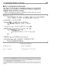
Common Time Stepp<strong>in</strong>g<br />
A common time-stepp<strong>in</strong>g mechanism is used for all one-step methods. The rout<strong>in</strong>e handles a<br />
number of different criteria <strong>in</strong>clud<strong>in</strong>g:<br />
† Step sizes <strong>in</strong> a numerical <strong>in</strong>tegration do not become too small <strong>in</strong> value, which may happen<br />
<strong>in</strong> solv<strong>in</strong>g stiff systems<br />
† Step sizes do not change sign unexpectedly, which may be a consequence of user programm<strong>in</strong>g<br />
error<br />
† Step sizes are not <strong>in</strong>creased after a step rejection<br />
† Step sizes are not decreased drastically toward the end of an <strong>in</strong>tegration<br />
† Specified (or detected) s<strong>in</strong>gularities are handled by restart<strong>in</strong>g the <strong>in</strong>tegration<br />
† Divergence of iterations <strong>in</strong> implicit methods (e.g. us<strong>in</strong>g fixed, large step sizes)<br />
† Unrecoverable <strong>in</strong>tegration errors (e.g. numerical exceptions)<br />
† Round<strong>in</strong>g error feedback (compensated summation) is particularly advantageous for highorder<br />
methods or methods that conserve specific quantities dur<strong>in</strong>g the numerical <strong>in</strong>tegration<br />
Data Encapsulation<br />
Each method has its own data object that conta<strong>in</strong>s <strong>in</strong>formation that is needed for the <strong>in</strong>vocation<br />
of the method. This <strong>in</strong>cludes, but is not limited to, coefficients, workspaces, step-size control<br />
parameters, step-size acceptance/rejection <strong>in</strong>formation, and Jacobian matrices. This is a general -<br />
ization of the ideas used <strong>in</strong> codes like LSODA ([H83], [P83]).
Method Hierarchy<br />
Methods are reentrant and hierarchical, mean<strong>in</strong>g that one method can call another. This is a<br />
generalization of the ideas used <strong>in</strong> the Generic ODE <strong>Solv<strong>in</strong>g</strong> System, Godess (see [O95], [O98]<br />
and the references there<strong>in</strong>), which is implemented <strong>in</strong> C++.<br />
Initial Design<br />
The orig<strong>in</strong>al method framework design allowed a number of methods to be <strong>in</strong>voked <strong>in</strong> the solver.<br />
NDSolve ö “ExplicitRungeKutta“<br />
NDSolve ö “ImplicitRungeKutta“<br />
First Revision<br />
This was later extended to allow one method to call another <strong>in</strong> a sequential fashion, with an<br />
arbitrary number of levels of nest<strong>in</strong>g.<br />
NDSolve ö “Extrapolation“ ö “ExplicitMidpo<strong>in</strong>t“<br />
The construction of compound <strong>in</strong>tegration methods is particularly useful <strong>in</strong> geometric numerical<br />
<strong>in</strong>tegration.<br />
NDSolve ö “Projection“ ö “ExplicitRungeKutta“<br />
Second Revision<br />
A more general tree <strong>in</strong>vocation process was required to implement composition methods.<br />
NDSolve ö “Composition“<br />
ç “ExplicitEuler“<br />
ª ª<br />
ö “ImplicitEuler“<br />
ª ª<br />
é “ExplicitEuler“<br />
This is an example of a method composed with its adjo<strong>in</strong>t.<br />
<strong>Advanced</strong> <strong>Numerical</strong> <strong>Differential</strong> <strong>Equation</strong> <strong>Solv<strong>in</strong>g</strong> <strong>in</strong> <strong>Mathematica</strong> 13
14 <strong>Advanced</strong> <strong>Numerical</strong> <strong>Differential</strong> <strong>Equation</strong> <strong>Solv<strong>in</strong>g</strong> <strong>in</strong> <strong>Mathematica</strong><br />
Current State<br />
The tree <strong>in</strong>vocation process was extended to allow for a subfield to be solved by each method,<br />
<strong>in</strong>stead of the entire vector field.<br />
This example turns up <strong>in</strong> the ABC Flow subsection of "Composition and Splitt<strong>in</strong>g Methods for<br />
NDSolve".<br />
NDSolve ö “Splitt<strong>in</strong>g“ f = f1 + f2<br />
User Extensibility<br />
ç “LocallyExact“ f1<br />
ö “ImplicitMidpo<strong>in</strong>t“ f2<br />
é “LocallyExact“ f1<br />
Built-<strong>in</strong> methods can be used as build<strong>in</strong>g blocks for the efficient construction of special-purpose<br />
(compound) <strong>in</strong>tegrators. User-def<strong>in</strong>ed methods can also be added.<br />
Method Classes<br />
Methods such as “ExplicitRungeKutta“ <strong>in</strong>clude a number of schemes of different orders.<br />
Moreover, alternative coefficient choices can be specified by the user. This is a generalization of<br />
the ideas found <strong>in</strong> RKSUITE [BGS93].<br />
Automatic Selection and User Controllability<br />
The framework provides automatic step-size selection and method-order selection. Methods are<br />
user-configurable via method options.<br />
For example a user can select the class of “ExplicitRungeKutta“ methods, and the code will<br />
automatically attempt to ascerta<strong>in</strong> the "optimal" order accord<strong>in</strong>g to the problem, the relative<br />
and absolute local error tolerances, and the <strong>in</strong>itial step-size estimate.
Here is a list of options appropriate for “ExplicitRungeKutta“.<br />
In[1]:= Options@NDSolve`ExplicitRungeKuttaD<br />
Out[1]= :Coefficients Ø EmbeddedExplicitRungeKuttaCoefficients, DifferenceOrder Ø Automatic,<br />
EmbeddedDifferenceOrder Ø Automatic, StepSizeControlParameters Ø Automatic,<br />
StepSizeRatioBounds Ø : 1<br />
, 4>, StepSizeSafetyFactors Ø Automatic, StiffnessTest Ø Automatic><br />
8<br />
MethodMonitor<br />
In order to illustrate the low-level behaviour of some methods, such as stiffness switch<strong>in</strong>g or<br />
order variation that occurs at run time , a new “MethodMonitor“ has been added.<br />
This fits between the relatively coarse resolution of “StepMonitor“ and the f<strong>in</strong>e resolution of<br />
“EvaluationMonitor“ .<br />
StepMonitor<br />
MethodMonitor<br />
EvaluationMonitor<br />
This feature is not officially documented and the functionality may change <strong>in</strong> future versions.<br />
Shared Features<br />
These features are not necessarily restricted to NDSolve s<strong>in</strong>ce they can also be used for other<br />
types of numerical methods.<br />
<strong>Advanced</strong> <strong>Numerical</strong> <strong>Differential</strong> <strong>Equation</strong> <strong>Solv<strong>in</strong>g</strong> <strong>in</strong> <strong>Mathematica</strong> 15<br />
† Function evaluation is performed us<strong>in</strong>g a <strong>Numerical</strong>Function that dynamically changes<br />
type as needed, such as when IEEE float<strong>in</strong>g-po<strong>in</strong>t overflow or underflow occurs. It also calls<br />
<strong>Mathematica</strong>'s compiler Compile for efficiency when appropriate.<br />
† Jacobian evaluation uses symbolic differentiation or f<strong>in</strong>ite difference approximations, <strong>in</strong>clud<strong>in</strong>g<br />
automatic or user-specifiable sparsity detection.<br />
† Dense l<strong>in</strong>ear algebra is based on LAPACK, and sparse l<strong>in</strong>ear algebra uses special-purpose<br />
packages such as UMFPACK.
16 <strong>Advanced</strong> <strong>Numerical</strong> <strong>Differential</strong> <strong>Equation</strong> <strong>Solv<strong>in</strong>g</strong> <strong>in</strong> <strong>Mathematica</strong><br />
† Common subexpressions <strong>in</strong> the numerical evaluation of the function represent<strong>in</strong>g a differential<br />
system are detected and collected to avoid repeated work.<br />
† Other support<strong>in</strong>g functionality that has been implemented is described <strong>in</strong> "Norms <strong>in</strong><br />
NDSolve".<br />
This system dynamically switches type from real to complex dur<strong>in</strong>g the numerical <strong>in</strong>tegration,<br />
automatically recompil<strong>in</strong>g as needed.<br />
In[2]:= y@1 ê 2D ê. NDSolve@8y‘@tD ã Sqrt@y@tDD - 1, y@0D ã 1 ê 10
ODE Integration Methods<br />
Methods<br />
"ExplicitRungeKutta" Method for NDSolve<br />
Introduction<br />
This loads packages conta<strong>in</strong><strong>in</strong>g some test problems and utility functions.<br />
In[3]:= Needs@“<strong>Differential</strong><strong>Equation</strong>s`NDSolveProblems`“D;<br />
Needs@“<strong>Differential</strong><strong>Equation</strong>s`NDSolveUtilities`“D;<br />
Euler's Method<br />
One of the first and simplest methods for solv<strong>in</strong>g <strong>in</strong>itial value problems was proposed by Euler:<br />
yn+1 = yn + h f Htn, ynL.<br />
Euler's method is not very accurate.<br />
Local accuracy is measured by how high terms are matched with the Taylor expansion of the<br />
solution. Euler's method is first-order accurate, so that errors occur one order higher start<strong>in</strong>g at<br />
powers of h2 .<br />
Euler's method is implemented <strong>in</strong> NDSolve as “ExplicitEuler“.<br />
In[5]:= NDSolve@8y‘@tD ã -y@tD, y@0D ã 1
18 <strong>Advanced</strong> <strong>Numerical</strong> <strong>Differential</strong> <strong>Equation</strong> <strong>Solv<strong>in</strong>g</strong> <strong>in</strong> <strong>Mathematica</strong><br />
For example, consider the one-step formulation of the midpo<strong>in</strong>t method.<br />
k1 = f Htn, ynL<br />
k2 = f Jtn + 1<br />
2 h, yn + 1<br />
h k1N<br />
2<br />
yn+1 = yn + h k2<br />
The midpo<strong>in</strong>t method can be shown to have a local error of OIh 3 M, so it is second-order accurate.<br />
The midpo<strong>in</strong>t method is implemented <strong>in</strong> NDSolve as “ExplicitMidpo<strong>in</strong>t“.<br />
In[6]:= NDSolve@8y‘@tD ã -y@tD, y@0D ã 1
It has become customary to denote the method coefficients c = @ciD T , b = @biD T , and A = Aai,jE us<strong>in</strong>g a<br />
Butcher table, which has the follow<strong>in</strong>g form for explicit Runge|Kutta methods:<br />
0 0 0 0 0<br />
c2 a2,1 0 0 0<br />
ª ª ª ª ª<br />
cs as,1 as,2 as,s-1 0<br />
b1 b2 bs-1 bs<br />
The row-sum conditions can be visualized as summ<strong>in</strong>g across the rows of the table.<br />
Notice that a consequence of explicitness is c1 = 0, so that the function is sampled at the beg<strong>in</strong>-<br />
n<strong>in</strong>g of the current <strong>in</strong>tegration step.<br />
Example<br />
The Butcher table for the explicit midpo<strong>in</strong>t method (1) is given by:<br />
0 0 0<br />
1<br />
2<br />
1<br />
2 0<br />
0 1<br />
FSAL Schemes<br />
A particularly <strong>in</strong>terest<strong>in</strong>g special class of explicit Runge|Kutta methods, used <strong>in</strong> most modern<br />
codes, are those for which the coefficients have a special structure known as First Same As Last<br />
(FSAL):<br />
as,i = bi, i = 1, …, s - 1 and bs = 0.<br />
For consistent FSAL schemes the Butcher table (3) has the form:<br />
0 0 0 0 0<br />
c2 a2,1 0 0 0<br />
ª ª ª ª ª<br />
cs-1 as-1,1 as-1,2 0 0<br />
1 b1 b2 bs-1 0<br />
b1 b2 bs-1 0<br />
The advantage of FSAL methods is that the function value ks at the end of one <strong>in</strong>tegration step<br />
is the same as the first function value k1 at the next <strong>in</strong>tegration step.<br />
<strong>Advanced</strong> <strong>Numerical</strong> <strong>Differential</strong> <strong>Equation</strong> <strong>Solv<strong>in</strong>g</strong> <strong>in</strong> <strong>Mathematica</strong> 19<br />
(3)<br />
(1)<br />
(1)<br />
(2)
20 <strong>Advanced</strong> <strong>Numerical</strong> <strong>Differential</strong> <strong>Equation</strong> <strong>Solv<strong>in</strong>g</strong> <strong>in</strong> <strong>Mathematica</strong><br />
The function values at the beg<strong>in</strong>n<strong>in</strong>g and end of each <strong>in</strong>tegration step are required anyway<br />
when construct<strong>in</strong>g the Interpolat<strong>in</strong>gFunction that is used for dense output <strong>in</strong> NDSolve.<br />
Embedded Pairs and Local Error Estimation<br />
An efficient means of obta<strong>in</strong><strong>in</strong>g local error estimates for adaptive step-size control is to consider<br />
two methods of different orders p and p ` that share the same coefficient matrix (and hence<br />
function values).<br />
0 0 0 0 0<br />
c2 a2,1 0 0 0<br />
ª ª ª 0 ª<br />
cs-1 as-1,1 as-1,2 0 0<br />
cs as,1 as,2 as,s-1 0<br />
b1 b2 bs-1 bs<br />
b ` 1 b ` 2 b ` s-1 b ` s<br />
These give two solutions:<br />
s<br />
yn+1 = yn + h ⁄ i=1 bi ki<br />
y ` n+1 = yn<br />
s `<br />
+ h ⁄ i=1 bi ki<br />
A commonly used notation is pHp ` L, typically with p ` = p - 1 or p ` = p + 1.<br />
In most modern codes, <strong>in</strong>clud<strong>in</strong>g the default choice <strong>in</strong> NDSolve, the solution is advanced with<br />
the more accurate formula so that p ` = p - 1, which is known as local extrapolation.<br />
The vector of coefficients e = Bb1 - b ` 1, b2 - b ` 2, …, bs - b ` sF T<br />
(1)<br />
(2)<br />
(3)<br />
gives an error estimator avoid<strong>in</strong>g subtrac-<br />
tive cancellation of yn <strong>in</strong> float<strong>in</strong>g-po<strong>in</strong>t arithmetic when form<strong>in</strong>g the difference between (2) and<br />
(3).<br />
s<br />
errn = h ‚<br />
i=1<br />
ei ki<br />
The quantity °errn¥ gives a scalar measure of the error that can be used for step size selection.
Step Control<br />
The classical Integral (or I) step-size controller uses the formula:<br />
hn+1 = hn K Tol<br />
±err nµ O1íp~<br />
where p ~<br />
= m<strong>in</strong>Ip ` , pM + 1.<br />
The error estimate is therefore used to determ<strong>in</strong>e the next step size to use from the current<br />
step size.<br />
The notation Tolê°errn¥ is expla<strong>in</strong>ed with<strong>in</strong> "Norms <strong>in</strong> NDSolve".<br />
Overview<br />
Explicit Runge|Kutta pairs of orders 2(1) through 9(8) have been implemented.<br />
Formula pairs have the follow<strong>in</strong>g properties:<br />
† First Same As Last strategy.<br />
† Local extrapolation mode, that is, the higher-order formula is used to propagate the<br />
solution.<br />
† Stiffness detection capability (see "StiffnessTest Method Option for NDSolve").<br />
† Proportional-Integral step-size controller for stiff and quasi-stiff systems [G91].<br />
Optimal formula pairs of orders 2(1), 3(2), and 4(3) subject to the already stated requirements<br />
have been derived us<strong>in</strong>g <strong>Mathematica</strong>, and are described <strong>in</strong> [SS04].<br />
The 5(4) pair selected is due to Bogacki and Shamp<strong>in</strong>e [BS89b, S94] and the 6(5), 7(6), 8(7),<br />
and 9(8) pairs are due to Verner.<br />
For the selection of higher-order pairs, issues such as local truncation error ratio and stability<br />
region compatibility should be considered (see [S94]). Various tools have been written to<br />
assess these qualitative features.<br />
<strong>Advanced</strong> <strong>Numerical</strong> <strong>Differential</strong> <strong>Equation</strong> <strong>Solv<strong>in</strong>g</strong> <strong>in</strong> <strong>Mathematica</strong> 21<br />
Methods are <strong>in</strong>terchangeable so that, for example, it is possible to substitute the 5(4) method<br />
of Bogacki and Shamp<strong>in</strong>e with a method of Dormand and Pr<strong>in</strong>ce.<br />
Summation of the method stages is implemented us<strong>in</strong>g level 2 BLAS which is often highly<br />
optimized for particular processors and can also take advantage of multiple cores.<br />
(1)
22 <strong>Advanced</strong> <strong>Numerical</strong> <strong>Differential</strong> <strong>Equation</strong> <strong>Solv<strong>in</strong>g</strong> <strong>in</strong> <strong>Mathematica</strong><br />
Example<br />
Def<strong>in</strong>e the Brusselator ODE problem, which models a chemical reaction.<br />
In[7]:= system = GetNDSolveProblem@“BrusselatorODE“D<br />
Out[7]= NDSolveProblemB:9HY1L £ @TD ã 1 - 4 Y1@TD + Y1@TD 2 Y2@TD, HY2L £ @TD ã 3 Y1@TD - Y1@TD 2 Y2@TD=, :Y1@0D ã 3<br />
, Y2@0D ã 3>, 8Y1@TD, Y2@TD
You also may want to compare some of the different methods to see how they perform for a<br />
specific problem.<br />
Utilities<br />
You will make use of a utility function CompareMethods for compar<strong>in</strong>g various methods. Some<br />
useful NDSolve features of this function for compar<strong>in</strong>g methods are:<br />
† The option EvaluationMonitor, which is used to count the number of function evaluations<br />
† The option StepMonitor, which is used to count the number of accepted and rejected<br />
<strong>in</strong>tegration steps<br />
This displays the results of the method comparison us<strong>in</strong>g a GridBox.<br />
In[12]:= TabulateResults@labels_List, names_List, data_ListD :=<br />
DisplayForm@<br />
FrameBox@<br />
GridBox@<br />
Apply@8labels, ÒÒ< &, MapThread@Prepend, 8data, names Automatic, the code will automatically attempt to<br />
choose the optimal order method for the <strong>in</strong>tegration.<br />
<strong>Advanced</strong> <strong>Numerical</strong> <strong>Differential</strong> <strong>Equation</strong> <strong>Solv<strong>in</strong>g</strong> <strong>in</strong> <strong>Mathematica</strong> 23<br />
Two algorithms have been implemented for this purpose and are described with<strong>in</strong><br />
"SymplecticPartitionedRungeKutta Method for NDSolve".
24 <strong>Advanced</strong> <strong>Numerical</strong> <strong>Differential</strong> <strong>Equation</strong> <strong>Solv<strong>in</strong>g</strong> <strong>in</strong> <strong>Mathematica</strong><br />
Example 1<br />
Here is an example that compares built-<strong>in</strong> methods of various orders, together with the method<br />
that is selected automatically.<br />
This selects the order of the methods to choose between and makes a list of method options to<br />
pass to NDSolve.<br />
In[15]:= orders = Jo<strong>in</strong>@Range@2, 9D, 8Automatic
This selects the order of the methods to choose between and makes a list of method options to<br />
pass to NDSolve.<br />
In[20]:= orders = Jo<strong>in</strong>@Range@4, 9D, 8Automatic
26 <strong>Advanced</strong> <strong>Numerical</strong> <strong>Differential</strong> <strong>Equation</strong> <strong>Solv<strong>in</strong>g</strong> <strong>in</strong> <strong>Mathematica</strong><br />
The Classical Runge|Kutta Method<br />
This shows how to def<strong>in</strong>e the coefficients of the classical explicit Runge|Kutta method of order<br />
four, approximated to precision p.<br />
In[24]:= crkamat = 881 ê 2
This def<strong>in</strong>es the function for comput<strong>in</strong>g the coefficients to a desired precision.<br />
In[33]:= Fehlbergamat = 8<br />
81 ê 4
28 <strong>Advanced</strong> <strong>Numerical</strong> <strong>Differential</strong> <strong>Equation</strong> <strong>Solv<strong>in</strong>g</strong> <strong>in</strong> <strong>Mathematica</strong><br />
Method Comparison<br />
Here you solve a system us<strong>in</strong>g several explicit Runge|Kutta pairs.<br />
For the Fehlberg 4(5) pair, the option “EmbeddedDifferenceOrder“ is used to specify the<br />
order of the embedded method.<br />
In[44]:= Fehlberg45 = 8“ExplicitRungeKutta“, “Coefficients“ Ø FehlbergCoefficients,<br />
“DifferenceOrder“ Ø 4, “EmbeddedDifferenceOrder“ Ø 5, “StiffnessTest“ Ø False
This def<strong>in</strong>ition is optional s<strong>in</strong>ce the method <strong>in</strong> fact has no data. However, any expression can be<br />
stored <strong>in</strong>side the data object. For example, the coefficients could be approximated here to avoid<br />
coercion from rational to float<strong>in</strong>g-po<strong>in</strong>t numbers at each <strong>in</strong>tegration step.<br />
In[52]:= ClassicalRungeKutta ê:<br />
NDSolve`InitializeMethod@ClassicalRungeKutta, __D := ClassicalRungeKutta@D;<br />
The actual method implementation is written us<strong>in</strong>g a stepp<strong>in</strong>g procedure.<br />
In[53]:= ClassicalRungeKutta@___D@“Step“@f_, t_, h_, y_, yp_DD :=<br />
Block@8deltay, k1, k2, k3, k4
30 <strong>Advanced</strong> <strong>Numerical</strong> <strong>Differential</strong> <strong>Equation</strong> <strong>Solv<strong>in</strong>g</strong> <strong>in</strong> <strong>Mathematica</strong><br />
L<strong>in</strong>ear Stability<br />
Consider apply<strong>in</strong>g a Runge|Kutta method to a l<strong>in</strong>ear scalar equation known as Dahlquist's<br />
equation:<br />
The result is a rational function of polynomials RHzL where z = h l (see for example [L87]).<br />
This utility function f<strong>in</strong>ds the l<strong>in</strong>ear stability function RHzL for Runge|Kutta methods. The form<br />
depends on the coefficients and is a polynomial if the Runge|Kutta method is explicit.<br />
Here is the stability function for the fifth-order scheme <strong>in</strong> the Dormand|Pr<strong>in</strong>ce 5(4) pair.<br />
In[55]:= DOPRIsf = RungeKuttaL<strong>in</strong>earStabilityFunction@DOPRIamat, DOPRIbvec, zD<br />
Out[55]= 1 + z + z2<br />
2<br />
+ z3<br />
6<br />
+ z4<br />
+<br />
24<br />
z5<br />
+<br />
120<br />
z6<br />
600<br />
This function f<strong>in</strong>ds the l<strong>in</strong>ear stability function RHzL for Runge|Kutta methods. The form depends<br />
on the coefficients and is a polynomial if the Runge|Kutta method is explicit.<br />
The follow<strong>in</strong>g package is useful for visualiz<strong>in</strong>g l<strong>in</strong>ear stability regions for numerical methods for<br />
differential equations.<br />
In[56]:= Needs@“FunctionApproximations`“D;<br />
You can now visualize the absolute stability region †RHzL§ = 1.<br />
In[57]:= OrderStarPlot@DOPRIsf, 1, zD<br />
Out[57]=<br />
y £ HtL = l yHtL, l œ , ReHlL < 0.<br />
(1)
Depend<strong>in</strong>g on the magnitude of l <strong>in</strong> (1), if you choose the step size h such that †RHh lL§ < 1, then<br />
errors <strong>in</strong> successive steps will be damped, and the method is said to be absolutely stable.<br />
If †RHh lL§ > 1, then step-size selection will be restricted by stability and not by local accuracy.<br />
Stiffness Detection<br />
The device for stiffness detection that is used with the option “StiffnessTest“ is described<br />
with<strong>in</strong> "StiffnessTest Method Option for NDSolve".<br />
Recast <strong>in</strong> terms of explicit Runge|Kutta methods, the condition for stiffness detection can be<br />
formulated as:<br />
l ~<br />
= ±ks-k s-1µ<br />
±gs-g s-1µ<br />
with gi and ki def<strong>in</strong>ed <strong>in</strong> (1).<br />
The difference gs - gs-1 can be shown to correspond to a number of applications of the power<br />
method applied to h J.<br />
The difference is therefore a good approximation of the eigenvector correspond<strong>in</strong>g to the lead-<br />
<strong>in</strong>g eigenvalue.<br />
The product £h l ~<br />
ß gives an estimate that can be compared to the stability boundary <strong>in</strong> order to<br />
detect stiffness.<br />
An s-stage explicit Runge|Kutta has a form suitable for (2) if cs-1 = cs = 1.<br />
0 0 0 0 0<br />
c2 a2,1 0 0 0<br />
ª ª ª ª ª<br />
1 as-1,1 as-1,2 0 0<br />
1 as,1 as,2 as,s-1 0<br />
b1 b2 bs-1 bs<br />
The default embedded pairs used <strong>in</strong> “ExplicitRungeKutta“ all have the form (3).<br />
An important po<strong>in</strong>t is that (2) is very cheap and convenient; it uses already available <strong>in</strong>forma-<br />
tion from the <strong>in</strong>tegration and requires no additional function evaluations.<br />
Another advantage of (3) is that it is straightforward to make use of consistent FSAL<br />
methods (1).<br />
<strong>Advanced</strong> <strong>Numerical</strong> <strong>Differential</strong> <strong>Equation</strong> <strong>Solv<strong>in</strong>g</strong> <strong>in</strong> <strong>Mathematica</strong> 31<br />
(2)<br />
(3)
32 <strong>Advanced</strong> <strong>Numerical</strong> <strong>Differential</strong> <strong>Equation</strong> <strong>Solv<strong>in</strong>g</strong> <strong>in</strong> <strong>Mathematica</strong><br />
Another advantage of (3) is that it is straightforward to make use of consistent FSAL<br />
methods (1).<br />
Examples<br />
Select a stiff system model<strong>in</strong>g a chemical reaction.<br />
In[58]:= system = GetNDSolveProblem@“Robertson“D;<br />
This applies a built-<strong>in</strong> explicit Runge|Kutta method to the stiff system.<br />
By default stiffness detection is enabled, s<strong>in</strong>ce it only has a small impact on the runn<strong>in</strong>g time.<br />
In[59]:= NDSolve@system, Method Ø “ExplicitRungeKutta“D;<br />
NDSolve::ndstf :<br />
At T == 0.012555829610695773`, system appears to be stiff. Methods Automatic, BDF or<br />
StiffnessSwitch<strong>in</strong>g may be more appropriate. à<br />
The coefficients of the Dormand|Pr<strong>in</strong>ce 5(4) pair are of the form (3) so stiffness detection is<br />
enabled.<br />
In[60]:= NDSolve@system, Method Ø 8“ExplicitRungeKutta“,<br />
“DifferenceOrder“ Ø 5, “Coefficients“ Ø DOPRICoefficients
The follow<strong>in</strong>g def<strong>in</strong>ition sets the value of the l<strong>in</strong>ear stability boundary.<br />
In[64]:= DOPRICoefficients@5D@“L<strong>in</strong>earStabilityBoundary“D =<br />
Root@600 + 300 * Ò1 + 100 * Ò1^2 + 25 * Ò1^3 + 5 * Ò1^4 + Ò1^5 &, 1, 0D;<br />
Us<strong>in</strong>g the new value for this example does not affect the time at which stiffness is detected.<br />
In[65]:= NDSolve@system, Method Ø 8“ExplicitRungeKutta“,<br />
“DifferenceOrder“ Ø 5, “Coefficients“ Ø DOPRICoefficients Automatic checks to see if the method coefficients<br />
provide a stiffness detection capability; if they do, then stiffness detection is enabled.<br />
Step Control Revisited<br />
There are some reasons to look at alternatives to the standard Integral step controller (1) when<br />
consider<strong>in</strong>g mildly stiff problems.<br />
This system models a chemical reaction.<br />
In[66]:= system = GetNDSolveProblem@“Robertson“D;<br />
This def<strong>in</strong>es an explicit Runge|Kutta method based on the Dormand|Pr<strong>in</strong>ce coefficients that does<br />
not use stiffness detection.<br />
In[67]:= IERK = 8“ExplicitRungeKutta“, “Coefficients“ Ø DOPRICoefficients,<br />
“DifferenceOrder“ Ø 5, “StiffnessTest“ Ø False
34 <strong>Advanced</strong> <strong>Numerical</strong> <strong>Differential</strong> <strong>Equation</strong> <strong>Solv<strong>in</strong>g</strong> <strong>in</strong> <strong>Mathematica</strong><br />
It can be studied by match<strong>in</strong>g the l<strong>in</strong>ear stability regions for the high- and low-order methods <strong>in</strong><br />
an embedded pair.<br />
One approach to address<strong>in</strong>g the oscillation is to derive special methods, but this compromises<br />
the local accuracy.<br />
PI Step Control<br />
An appeal<strong>in</strong>g alternative to Integral step control (1) is Proportional-Integral or PI step control.<br />
In this case the step size is selected us<strong>in</strong>g the local error <strong>in</strong> two successive <strong>in</strong>tegration steps<br />
accord<strong>in</strong>g to the formula:<br />
hn+1 = hn K Tol<br />
±errnµ Ok 1íp ~<br />
K ±errn-1µ ±errnµ O<br />
k2íp ~<br />
This has the effect of damp<strong>in</strong>g and hence gives a smoother step-size sequence.<br />
Note that Integral step control (1) is a special case of (1) and is used if a step is rejected:<br />
k1 = 1, k2 = 0 .<br />
The option “StepSizeControlParameters“ -> 8k1, k2< can be used to specify the values of k1<br />
and k2.<br />
The scaled error estimate <strong>in</strong> (1) is taken to be °errn-1¥ = °errn¥ for the first <strong>in</strong>tegration step.<br />
Examples<br />
Stiff Problem<br />
This def<strong>in</strong>es a method similar to IERK that uses the option “StepSizeControlParameters“ to<br />
specify a PI controller.<br />
Here you use generic control parameters suggested by Gustafsson:<br />
k1 = 3ê10, k2 = 2ê5<br />
This specifies the step-control parameters.<br />
In[70]:= PIERK = 8“ExplicitRungeKutta“,<br />
“Coefficients“ Ø DOPRICoefficients, “DifferenceOrder“ Ø 5,<br />
“StiffnessTest“ Ø False, “StepSizeControlParameters“ Ø 83 ê 10, 2 ê 5
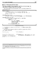
<strong>Solv<strong>in</strong>g</strong> the system aga<strong>in</strong>, it can be observed that the step-size sequence is now much<br />
smoother.<br />
In[71]:= pisol = NDSolve@system, Method Ø PIERKD;<br />
StepDataPlot@pisolD<br />
Out[72]=<br />
0.0015<br />
0.0010<br />
Nonstiff Problem<br />
0.00 0.05 0.10 0.15 0.20 0.25 0.30<br />
In general the I step controller (1) is able to take larger steps for a nonstiff problem than the PI<br />
step controller (1) as the follow<strong>in</strong>g example illustrates.<br />
Select and solve a nonstiff system us<strong>in</strong>g the I step controller.<br />
In[73]:= system = GetNDSolveProblem@“BrusselatorODE“D;<br />
In[74]:= isol = NDSolve@system, Method Ø IERKD;<br />
StepDataPlot@isolD<br />
Out[75]=<br />
0.200<br />
0.150<br />
0.100<br />
0.070<br />
0.050<br />
0.030<br />
0.020<br />
0.015<br />
0 5 10 15 20<br />
Us<strong>in</strong>g the PI step controller the step sizes are slightly smaller.<br />
In[76]:= pisol = NDSolve@system, Method Ø PIERKD;<br />
StepDataPlot@pisolD<br />
Out[77]=<br />
0.150<br />
0.100<br />
0.070<br />
0.050<br />
0.030<br />
0.020<br />
0.015<br />
0.010<br />
0 5 10 15 20<br />
For this reason, the default sett<strong>in</strong>g for “StepSizeControlParameters“ is Automatic , which is<br />
<strong>in</strong>terpreted as:<br />
† Use the I step controller (1) if “StiffnessTest“ -> False.<br />
† Use the PI step controller (1) if “StiffnessTest“ -> True.<br />
<strong>Advanced</strong> <strong>Numerical</strong> <strong>Differential</strong> <strong>Equation</strong> <strong>Solv<strong>in</strong>g</strong> <strong>in</strong> <strong>Mathematica</strong> 35
36 <strong>Advanced</strong> <strong>Numerical</strong> <strong>Differential</strong> <strong>Equation</strong> <strong>Solv<strong>in</strong>g</strong> <strong>in</strong> <strong>Mathematica</strong><br />
F<strong>in</strong>e-Tun<strong>in</strong>g<br />
Instead of us<strong>in</strong>g (1) directly, it is common practice to use safety factors to ensure that the error<br />
is acceptable at the next step with high probability, thereby prevent<strong>in</strong>g unwanted step<br />
rejections.<br />
The option “StepSizeSafetyFactors“ -> 8s1, s2< specifies the safety factors to use <strong>in</strong> the step-<br />
size estimate so that (1) becomes:<br />
hn+1 = hn s1 K s2 Tol<br />
±errnµ Ok 1íp ~<br />
K ±errn-1µ ±errnµ O<br />
k2íp ~<br />
.<br />
Here s1 is an absolute factor and s2 typically scales with the order of the method.<br />
The option “StepSizeRatioBounds“ -> 8srm<strong>in</strong>, srmax< specifies bounds on the next step size to<br />
take such that:<br />
srm<strong>in</strong> § ¢ h n+1<br />
hn<br />
§ srmax.<br />
Option summary<br />
option name default value<br />
"Coefficients" EmbeddedExplicÖ<br />
itRungeKuttaÖ<br />
Coefficients<br />
Options of the method “ExplicitRungeKutta“.<br />
specify the coefficients of the explicit<br />
Runge|Kutta method<br />
"DifferenceOrder" Automatic specify the order of local accuracy<br />
"EmbeddedDifferenceOrder" Automatic specify the order of the embedded method<br />
<strong>in</strong> a pair of explicit Runge|Kutta methods<br />
"StepSizeControlParameters<br />
"<br />
Automatic specify the PI step-control parameters (see<br />
(1))<br />
"StepSizeRatioBounds" : 1<br />
,4> specify the bounds on a relative change <strong>in</strong><br />
8<br />
the new step size (see (2))<br />
"StepSizeSafetyFactors" Automatic specify the safety factors to use <strong>in</strong> the step-<br />
size estimate (see (1))<br />
"StiffnessTest" Automatic specify whether to use the stiffness detec -<br />
tion capability<br />
(1)<br />
(2)
The default sett<strong>in</strong>g of Automatic for the option “DifferenceOrder“ selects the default coeffi-<br />
cient order based on the problem, <strong>in</strong>itial values-and local error tolerances, balanced aga<strong>in</strong>st the<br />
work of the method for each coefficient set.<br />
The default sett<strong>in</strong>g of Automatic for the option “EmbeddedDifferenceOrder“ specifies that the<br />
default order of the embedded method is one lower than the method order. This depends on<br />
the value of the “DifferenceOrder“ option.<br />
The default sett<strong>in</strong>g of Automatic for the option “StepSizeControlParameters“ uses the values<br />
81, 0< if stiffness detection is active and 83 ê 10, 2 ê 5< otherwise.<br />
The default sett<strong>in</strong>g of Automatic for the option “StepSizeSafetyFactors“ uses the values<br />
817 ê 20, 9 ê 10< if the I step controller (1) is used and 89 ê 10, 9 ê 10< if the PI step controller<br />
(1) is used. The step controller used depends on the values of the options<br />
“StepSizeControlParameters“ and “StiffnessTest“.<br />
The default sett<strong>in</strong>g of Automatic for the option “StiffnessTest“ will activate the stiffness test<br />
if if the coefficients have the form (3).<br />
"ImplicitRungeKutta" Method for NDSolve<br />
Introduction<br />
Implicit Runge|Kutta methods have a number of desirable properties.<br />
The Gauss|Legendre methods, for example, are self-adjo<strong>in</strong>t, mean<strong>in</strong>g that they provide the<br />
same solution when <strong>in</strong>tegrat<strong>in</strong>g forward or backward <strong>in</strong> time.<br />
This loads packages def<strong>in</strong><strong>in</strong>g some example problems and utility functions.<br />
In[3]:= Needs@“<strong>Differential</strong><strong>Equation</strong>s`NDSolveProblems`“D;<br />
Needs@“<strong>Differential</strong><strong>Equation</strong>s`NDSolveUtilities`“D;<br />
Coefficients<br />
A generic framework for implicit Runge|Kutta methods has been implemented. The focus so far<br />
is on methods with <strong>in</strong>terest<strong>in</strong>g geometric properties and currently covers the follow<strong>in</strong>g schemes:<br />
† “ImplicitRungeKuttaGaussCoefficients“<br />
† “ImplicitRungeKuttaLobattoIIIACoefficients“<br />
<strong>Advanced</strong> <strong>Numerical</strong> <strong>Differential</strong> <strong>Equation</strong> <strong>Solv<strong>in</strong>g</strong> <strong>in</strong> <strong>Mathematica</strong> 37
38 <strong>Advanced</strong> <strong>Numerical</strong> <strong>Differential</strong> <strong>Equation</strong> <strong>Solv<strong>in</strong>g</strong> <strong>in</strong> <strong>Mathematica</strong><br />
† “ImplicitRungeKuttaLobattoIIIBCoefficients“<br />
† “ImplicitRungeKuttaLobattoIIICCoefficients“<br />
† “ImplicitRungeKuttaRadauIACoefficients“<br />
† “ImplicitRungeKuttaRadauIIACoefficients“<br />
The derivation of the method coefficients can be carried out to arbitrary order and arbitrary<br />
precision.<br />
Coefficient Generation<br />
† Start with the def<strong>in</strong>ition of the polynomial, def<strong>in</strong><strong>in</strong>g the abscissas of the s stage coefficients.<br />
For example, the abscissas for Gauss|Legendre methods are def<strong>in</strong>ed as ds<br />
dx s x s H1 - xL s .<br />
† Univariate polynomial factorization gives the underly<strong>in</strong>g irreducible polynomials def<strong>in</strong><strong>in</strong>g the<br />
roots of the polynomials.<br />
† Root objects are constructed to represent the solutions (us<strong>in</strong>g unique root isolation and<br />
Jenk<strong>in</strong>s|Traub for the numerical approximation).<br />
† Root objects are then approximated numerically for precision coefficients.<br />
† Condition estimates for Vandermonde systems govern<strong>in</strong>g the coefficients yield the precision<br />
to take <strong>in</strong> approximat<strong>in</strong>g the roots numerically.<br />
† Specialized solvers for nonconfluent Vandermonde systems are then used to solve equations<br />
for the coefficients (see [GVL96]).<br />
† One step of iterative ref<strong>in</strong>ement is used to polish the approximate solutions and to check<br />
that the coefficients are obta<strong>in</strong>ed to the requested precision.<br />
This generates the coefficients for the two-stage fourth-order Gauss|Legendre method to 50<br />
decimal digits of precision.<br />
In[5]:= NDSolve`ImplicitRungeKuttaGaussCoefficients@4, 50D<br />
Out[5]= 8880.25000000000000000000000000000000000000000000000000,<br />
-0.038675134594812882254574390250978727823800875635063
In[6]:=<br />
This generates the coefficients for the two-stage fourth-order Gauss|Legendre method exactly.<br />
For high-order methods, generat<strong>in</strong>g the coefficients exactly can often take a very long time.<br />
NDSolve`ImplicitRungeKuttaGaussCoefficients@4, Inf<strong>in</strong>ityD<br />
Out[6]= ::: 1<br />
,<br />
4<br />
1<br />
3 - 2 3 >, :<br />
12<br />
1<br />
3 + 2 3 ,<br />
12<br />
1<br />
>>, :<br />
4<br />
1<br />
,<br />
2<br />
1<br />
>, :<br />
2<br />
1<br />
3 - 3 ,<br />
6<br />
1<br />
3 + 3 >><br />
6<br />
This generates the coefficients for the six-stage tenth-order RaduaIA implicit Runge|Kutta<br />
method to 20 decimal digits of precision.<br />
In[7]:= NDSolve`ImplicitRungeKuttaRadauIACoefficients@10, 20D<br />
Out[7]= 8880.040000000000000000000, -0.087618018725274235050,<br />
0.085317987638600293760, -0.055818078483298114837, 0.018118109569972056127
40 <strong>Advanced</strong> <strong>Numerical</strong> <strong>Differential</strong> <strong>Equation</strong> <strong>Solv<strong>in</strong>g</strong> <strong>in</strong> <strong>Mathematica</strong><br />
A plot of the error <strong>in</strong> the <strong>in</strong>variants shows an <strong>in</strong>crease as the <strong>in</strong>tegration proceeds.<br />
In[12]:= InvariantErrorPlot@<strong>in</strong>vs, vars, T, sol,<br />
PlotStyle Ø 8Red, Blue
The second <strong>in</strong>variant is conserved exactly (up to roundoff) s<strong>in</strong>ce the Gauss implicit Runge|Kutta<br />
method conserves quadratic <strong>in</strong>variants.<br />
In[14]:= InvariantErrorPlot@<strong>in</strong>vs, vars, T, sol,<br />
PlotStyle Ø 8Red, Blue<br />
“ImplicitRungeKuttaGaussCoefficients“, “DifferenceOrder“ Ø 2,<br />
“ImplicitSolver“ Ø 8“FixedPo<strong>in</strong>t“, “AccuracyGoal“ Ø Mach<strong>in</strong>ePrecision,<br />
“PrecisionGoal“ Ø Mach<strong>in</strong>ePrecision, “IterationSafetyFactor“ Ø 1
42 <strong>Advanced</strong> <strong>Numerical</strong> <strong>Differential</strong> <strong>Equation</strong> <strong>Solv<strong>in</strong>g</strong> <strong>in</strong> <strong>Mathematica</strong><br />
Option Summary<br />
"ImplicitRungeKutta" Options<br />
option name default value<br />
"Coefficients" "ImplicitRungeÖ<br />
KuttaGausÖ<br />
sCoefficiÖ<br />
ents"<br />
Options of the method “ImplicitRungeKutta“.<br />
The default sett<strong>in</strong>g of Automatic for the option “StepSizeSafetyFactors“ uses the values<br />
89 ê 10, 9 ê 10 specify the bounds on a relative change <strong>in</strong><br />
8<br />
the new step size<br />
"StepSizeSafetyFactors" Automatic specify the safety factors to use <strong>in</strong> the step<br />
size estimate
option name default value<br />
"JacobianEvaluationParameÖ<br />
ter"<br />
Options specific to the “Newton“ method of “ImplicitSolver“.<br />
"SymplecticPartitionedRungeKutta" Method for NDSolve<br />
Introduction<br />
When numerically solv<strong>in</strong>g Hamiltonian dynamical systems it is advantageous if the numerical<br />
method yields a symplectic map.<br />
† The phase space of a Hamiltonian system is a symplectic manifold on which there exists a<br />
natural symplectic structure <strong>in</strong> the canonically conjugate coord<strong>in</strong>ates.<br />
† The time evolution of a Hamiltonian system is such that the Po<strong>in</strong>caré <strong>in</strong>tegral <strong>in</strong>variants<br />
associated with the symplectic structure are preserved.<br />
† A symplectic <strong>in</strong>tegrator computes exactly, assum<strong>in</strong>g <strong>in</strong>f<strong>in</strong>ite precision arithmetic, the evolution<br />
of a nearby Hamiltonian, whose phase space structure is close to that of the orig<strong>in</strong>al<br />
system.<br />
If the Hamiltonian can be written <strong>in</strong> separable form, H Hp, qL = T HpL + V HqL, there exists an efficient<br />
class of explicit symplectic numerical <strong>in</strong>tegration methods.<br />
An important property of symplectic numerical methods when applied to Hamiltonian systems is<br />
that a nearby Hamiltonian is approximately conserved for exponentially long times (see [BG94],<br />
[HL97], and [R99]).<br />
Hamiltonian Systems<br />
Consider a differential equation<br />
dy<br />
dt = FHt, yL, yHt0L = y0.<br />
1<br />
1000<br />
<strong>Advanced</strong> <strong>Numerical</strong> <strong>Differential</strong> <strong>Equation</strong> <strong>Solv<strong>in</strong>g</strong> <strong>in</strong> <strong>Mathematica</strong> 43<br />
specify when to recompute the Jacobian<br />
matrix <strong>in</strong> Newton iterations<br />
"L<strong>in</strong>earSolveMethod" Automatic specify the l<strong>in</strong>ear solver to use <strong>in</strong> Newton<br />
iterations<br />
"LUDecompositionEvaluatioÖ<br />
nParameter"<br />
6<br />
5<br />
specify when to compute LU decomposi-<br />
tions <strong>in</strong> Newton iterations<br />
(1)
44 <strong>Advanced</strong> <strong>Numerical</strong> <strong>Differential</strong> <strong>Equation</strong> <strong>Solv<strong>in</strong>g</strong> <strong>in</strong> <strong>Mathematica</strong><br />
A d-degree of freedom Hamiltonian system is a particular <strong>in</strong>stance of (1) with<br />
y = Hp1, …, pd, q1 …, qdL T , where<br />
dy<br />
dt = J-1 “ H.<br />
Here “ represents the gradient operator:<br />
“= H∂ ê∂ p1, …, ∂ ê∂ pd, ∂ ê∂q1, … ∂ ê∂qdL T<br />
and J is the skew symmetric matrix:<br />
J =<br />
0 I<br />
-I 0<br />
where I and 0 are the identity and zero d×d matrices.<br />
The components of q are often referred to as position or coord<strong>in</strong>ate variables and the compo-<br />
nents of p as the momenta.<br />
If H is autonomous, dH êdt = 0. Then H is a conserved quantity that rema<strong>in</strong>s constant along<br />
solutions of the system. In applications, this usually corresponds to conservation of energy.<br />
A numerical method applied to a Hamiltonian system (2) is said to be symplectic if it produces a<br />
symplectic map. That is, let Hp * , q * L = yHp, qL be a C 1 transformation def<strong>in</strong>ed <strong>in</strong> a doma<strong>in</strong> W.:<br />
" Hp, qL œ W, y £ T J y £ = ∂Hp* , q * L T<br />
∂Hp, qL<br />
J ∂Hp* , q * L<br />
∂Hp, qL<br />
where the Jacobian of the transformation is:<br />
y £ = ∂Hp* , q * L<br />
∂Hp, qL =<br />
∂p *<br />
∂p<br />
∂q *<br />
∂p<br />
∂p *<br />
∂q<br />
∂q *<br />
∂q<br />
.<br />
= J<br />
The flow of a Hamiltonian system is depicted together with the projection onto the planes<br />
formed by canonically conjugate coord<strong>in</strong>ate and momenta pairs. The sum of the oriented areas<br />
rema<strong>in</strong>s constant as the flow evolves <strong>in</strong> time.<br />
(2)
q2<br />
pdq <br />
A2<br />
q1<br />
p2<br />
Partitioned Runge|Kutta Methods<br />
A1<br />
Ct<br />
pdq <br />
It is sometimes possible to <strong>in</strong>tegrate certa<strong>in</strong> components of (1) us<strong>in</strong>g one Runge|Kutta method<br />
and other components us<strong>in</strong>g a different Runge|Kutta method. The overall s-stage scheme is<br />
called a partitioned Runge|Kutta method and the free parameters are represented by two<br />
Butcher tableaux:<br />
a11 a1 s<br />
ª ª<br />
as1 ass<br />
b1 bs<br />
A11 A1 s<br />
ª ª<br />
As1 Ass<br />
B1 Bs<br />
Symplectic Partitioned Runge|Kutta (SPRK) Methods<br />
.<br />
For general Hamiltonian systems, symplectic Runge|Kutta methods are necessarily implicit.<br />
However, for separable Hamiltonians HHp, q, tL = THpL + VHq, tL there exist explicit schemes<br />
correspond<strong>in</strong>g to symplectic partitioned Runge|Kutta methods.<br />
<strong>Advanced</strong> <strong>Numerical</strong> <strong>Differential</strong> <strong>Equation</strong> <strong>Solv<strong>in</strong>g</strong> <strong>in</strong> <strong>Mathematica</strong> 45<br />
p1<br />
(1)
46 <strong>Advanced</strong> <strong>Numerical</strong> <strong>Differential</strong> <strong>Equation</strong> <strong>Solv<strong>in</strong>g</strong> <strong>in</strong> <strong>Mathematica</strong><br />
Instead of (1) the free parameters now take either the form:<br />
or the form:<br />
0 0 0<br />
b1 0 ª<br />
ª ª<br />
b1 bs-1 0<br />
b1 bs-1 bs<br />
b1 0 0<br />
b1 b2 ª<br />
ª ª ª<br />
b1 b2 bs<br />
b1 b2 bs<br />
B1 0 0<br />
B1 B2 ª<br />
ª ª ª<br />
B1 B2 Bs<br />
B1 B2 Bs<br />
0 0 0<br />
B1 0 ª<br />
ª ª<br />
B1 Bs-1 0<br />
B1 Bs-1 Bs<br />
.<br />
The 2 d free parameters of (2) are sometimes represented us<strong>in</strong>g the shorthand notation<br />
@b1, …, bsD HB1, …BsL.<br />
The differential system for a separable Hamiltonian system can be written as:<br />
dpi ∂VHq, tL<br />
= f Hq, tL = - ,<br />
dt ∂qi<br />
dqi ∂THpL<br />
= gHpL = , i = 1, …, d.<br />
dt<br />
∂ pi<br />
In general the force evaluations -∂VHq, tLê∂q are computationally dom<strong>in</strong>ant and (2) is preferred<br />
over (1) s<strong>in</strong>ce it is possible to save one force evaluation per time step when dense output is<br />
required.<br />
Standard Algorithm<br />
The structure of (2) permits a particularly simple implementation (see for example [SC94]).<br />
Algorithm 1 (Standard SPRK)<br />
P0 = pn<br />
Q1 = qn<br />
for i = 1, …, s<br />
(1)<br />
(2)
Pi = Pi-1 + hn+1 bi f HQi, tn + Ci hn+1L<br />
Qi+1 = Qi + hn+1 Bi gHPiL<br />
Return pn+1 = Ps and qn+1 = Qs+1.<br />
j-1<br />
The time-weights are given by: Cj = ⁄ i=1 Bi, j = 1, …, s.<br />
If Bs = 0 then Algorithm 1 effectively reduces to an s - 1 stage scheme s<strong>in</strong>ce it has the First Same<br />
As Last (FSAL) property.<br />
Example<br />
This loads some useful packages.<br />
In[1]:= Needs@“<strong>Differential</strong><strong>Equation</strong>s`NDSolveProblems`“D;<br />
Needs@“<strong>Differential</strong><strong>Equation</strong>s`NDSolveUtilities`“D;<br />
The Harmonic Oscillator<br />
The Harmonic oscillator is a simple Hamiltonian problem that models a material po<strong>in</strong>t attached<br />
to a spr<strong>in</strong>g. For simplicity consider the unit mass and spr<strong>in</strong>g constant for which the Hamiltonian<br />
is given <strong>in</strong> separable form:<br />
HHp, qL = THpL + VHqL = p 2 ë2 + q 2 ë2.<br />
The equations of motion are given by:<br />
Input<br />
dp<br />
dt<br />
∂H<br />
= - = -q,<br />
∂q<br />
dq<br />
dt<br />
∂H<br />
= = p, qH0L = 1, pH0L = 0.<br />
∂p<br />
In[3]:= system = GetNDSolveProblem@“HarmonicOscillator“D;<br />
eqs = 8system@“System“D, system@“InitialConditions“D
48 <strong>Advanced</strong> <strong>Numerical</strong> <strong>Differential</strong> <strong>Equation</strong> <strong>Solv<strong>in</strong>g</strong> <strong>in</strong> <strong>Mathematica</strong><br />
S<strong>in</strong>ce the method is dissipative, the trajectory spirals <strong>in</strong>to or away from the fixed po<strong>in</strong>t at the<br />
orig<strong>in</strong>.<br />
In[10]:= ParametricPlot@Evaluate@vars ê. First@soleeDD, Evaluate@timeD, PlotPo<strong>in</strong>ts Ø 100D<br />
Out[10]=<br />
6<br />
4<br />
2<br />
-6 -4 -2 2 4 6<br />
-2<br />
-4<br />
-6<br />
A dissipative method typically exhibits l<strong>in</strong>ear error growth <strong>in</strong> the value of the Hamiltonian.<br />
In[11]:= InvariantErrorPlot@H, vars, T, solee, PlotStyle Ø GreenD<br />
Out[11]=<br />
25<br />
20<br />
15<br />
10<br />
5<br />
0<br />
0 20 40 60 80 100<br />
Symplectic Method<br />
<strong>Numerical</strong>ly <strong>in</strong>tegrate the equations of motion for the Harmonic oscillator us<strong>in</strong>g a symplectic<br />
partitioned Runge|Kutta method.<br />
In[12]:= sol = NDSolve@eqs, vars, time, Method Ø 8“SymplecticPartitionedRungeKutta“,<br />
“DifferenceOrder“ Ø 2, “PositionVariables“ Ø 8Y1@TD
The solution is now a closed curve.<br />
In[13]:= ParametricPlot@Evaluate@vars ê. First@solDD, Evaluate@timeDD<br />
Out[13]= -1.0 -0.5 0.5 1.0<br />
1.0<br />
0.5<br />
-0.5<br />
-1.0<br />
In contrast to dissipative methods, symplectic <strong>in</strong>tegrators yield an error <strong>in</strong> the Hamiltonian that<br />
rema<strong>in</strong>s bounded.<br />
In[14]:= InvariantErrorPlot@H, vars, T, sol, PlotStyle Ø BlueD<br />
Out[14]=<br />
0.00020<br />
0.00015<br />
0.00010<br />
0.00005<br />
0.00000<br />
0 20 40 60 80 100<br />
Round<strong>in</strong>g Error Reduction<br />
<strong>Advanced</strong> <strong>Numerical</strong> <strong>Differential</strong> <strong>Equation</strong> <strong>Solv<strong>in</strong>g</strong> <strong>in</strong> <strong>Mathematica</strong> 49<br />
In certa<strong>in</strong> cases, lattice symplectic methods exist and can avoid step-by-step roundoff accumulation,<br />
but such an approach is not always possible [ET92].
50 <strong>Advanced</strong> <strong>Numerical</strong> <strong>Differential</strong> <strong>Equation</strong> <strong>Solv<strong>in</strong>g</strong> <strong>in</strong> <strong>Mathematica</strong><br />
Consider the previous example where the comb<strong>in</strong>ation of step size and order of the method is<br />
now chosen such that the error <strong>in</strong> the Hamiltonian is around the order of unit roundoff <strong>in</strong> IEEE<br />
double-precision arithmetic.<br />
In[15]:= solnoca = NDSolve@eqs, vars, time, Method Ø 8“SymplecticPartitionedRungeKutta“,<br />
“DifferenceOrder“ Ø 10, “PositionVariables“ Ø 8Y1@TD
yH,h<br />
et<br />
y ` H,h<br />
ey<br />
Many numerical methods for ord<strong>in</strong>ary differential equations <strong>in</strong>volve computations of the form:<br />
yn+1 = yn + dn<br />
where the <strong>in</strong>crements dn are usually smaller <strong>in</strong> magnitude than the approximations yn.<br />
Let eHxL denote the exponent and mHxL, 1 > mHxL ¥ 1ê b, the mantissa of a number x <strong>in</strong> precision p<br />
radix b arithmetic: x = mHxLä b eHxL .<br />
Then you can write:<br />
and<br />
yn = mHynLä b eHynL = yn h + yn l ä b eHdnL<br />
dn = mHdnLä b eHdnL = dn h + dn l ä b eHynL-p .<br />
Align<strong>in</strong>g accord<strong>in</strong>g to exponents these quantities can be represented pictorially as:<br />
d n l d n h<br />
y n l y n h<br />
where numbers on the left have a smaller scale than numbers on the right.<br />
Of <strong>in</strong>terest is an efficient way of comput<strong>in</strong>g the quantities d n l that effectively represent the radix<br />
b digits discarded due to the difference <strong>in</strong> the exponents of yn and dn.<br />
<strong>Advanced</strong> <strong>Numerical</strong> <strong>Differential</strong> <strong>Equation</strong> <strong>Solv<strong>in</strong>g</strong> <strong>in</strong> <strong>Mathematica</strong> 51
52 <strong>Advanced</strong> <strong>Numerical</strong> <strong>Differential</strong> <strong>Equation</strong> <strong>Solv<strong>in</strong>g</strong> <strong>in</strong> <strong>Mathematica</strong><br />
Compensated Summation<br />
The basic motivation for compensated summation is to simulate 2 n bit addition us<strong>in</strong>g only n bit<br />
arithmetic.<br />
Example<br />
This repeatedly adds a fixed amount to a start<strong>in</strong>g value. Cumulative roundoff error has a significant<br />
<strong>in</strong>fluence on the result.<br />
In[17]:= reps = 10 6 ;<br />
base = 0.;<br />
<strong>in</strong>c = 0.1;<br />
Do@base = base + <strong>in</strong>c, 8reps
By repeatedly feed<strong>in</strong>g back the round<strong>in</strong>g error from one sum <strong>in</strong>to the next, the effect of round<strong>in</strong>g<br />
errors is significantly reduced.<br />
In[22]:= err = 0.;<br />
base = 0.;<br />
<strong>in</strong>c = 0.1;<br />
Do@<br />
8base, err< =<br />
Developer`CompensatedPlus@base , <strong>in</strong>c, errD,<br />
8reps
54 <strong>Advanced</strong> <strong>Numerical</strong> <strong>Differential</strong> <strong>Equation</strong> <strong>Solv<strong>in</strong>g</strong> <strong>in</strong> <strong>Mathematica</strong><br />
<strong>Numerical</strong> Illustration<br />
Round<strong>in</strong>g Error Model<br />
The amount of expected roundoff error <strong>in</strong> the relative error of the Hamiltonian for the harmonic<br />
oscillator (1) will now be quantified. A probabilistic average case analysis is considered <strong>in</strong> prefer-<br />
ence to a worst case upper bound.<br />
For a one-dimensional random walk with equal probability of a deviation, the expected absolute<br />
distance after N steps is OI n M.<br />
The relative error for a float<strong>in</strong>g-po<strong>in</strong>t operation +, -, *, ê us<strong>in</strong>g IEEE round to nearest mode<br />
satisfies the follow<strong>in</strong>g bound [K93]:<br />
eround § 1ê2 b -p+1 º 1.11022ä10 -16<br />
where the base b = 2 is used for represent<strong>in</strong>g float<strong>in</strong>g-po<strong>in</strong>t numbers on the mach<strong>in</strong>e and p = 53<br />
for IEEE double-precision.<br />
Therefore the roundoff error after n steps is expected to be approximately:<br />
k e n<br />
for some constant k.<br />
In the examples that follow a constant step size of 1/25 is used and the <strong>in</strong>tegration is<br />
performed over the <strong>in</strong>terval [0, 80000] for a total of 2µ10 6 <strong>in</strong>tegration steps. The error <strong>in</strong> the<br />
Hamiltonian is sampled every 200 <strong>in</strong>tegration steps.<br />
The 8 th -order 15-stage (FSAL) method D of Yoshida is used. Similar results have been obta<strong>in</strong>ed<br />
for the 6 th -order 7-stage (FSAL) method A of Yoshida with the same number of <strong>in</strong>tegration<br />
steps and a step size of 1/160.<br />
Without Compensated Summation<br />
The relative error <strong>in</strong> the Hamiltonian is displayed here for the standard formulation <strong>in</strong> Algorithm<br />
1 (green) and for the <strong>in</strong>crement formulation <strong>in</strong> Algorithm 3 (red) for the Harmonic oscillator (1).
Algorithm 1 for a 15-stage method corresponds to n = 15µ2µ10 6 = 3µ10 7 .<br />
In the <strong>in</strong>cremental Algorithm 3 the <strong>in</strong>ternal stages are all of the order of the step size and the<br />
only significant round<strong>in</strong>g error occurs at the end of each <strong>in</strong>tegration step; thus n = 2µ10 6 , which<br />
is <strong>in</strong> good agreement with the observed improvement.<br />
This shows that for Algorithm 3, with sufficiently small step sizes, the round<strong>in</strong>g error growth is<br />
<strong>in</strong>dependent of the number of stages of the method, which is particularly advantageous for high<br />
order.<br />
With Compensated Summation<br />
The relative error <strong>in</strong> the Hamiltonian is displayed here for the <strong>in</strong>crement formulation <strong>in</strong> Algo-<br />
rithm 3 without compensated summation (red) and with compensated summation (blue) for the<br />
Harmonic oscillator (1).<br />
<strong>Advanced</strong> <strong>Numerical</strong> <strong>Differential</strong> <strong>Equation</strong> <strong>Solv<strong>in</strong>g</strong> <strong>in</strong> <strong>Mathematica</strong> 55<br />
Us<strong>in</strong>g compensated summation with Algorithm 3, the error growth appears to satisfy a random<br />
walk with deviation h e so that it has been reduced by a factor proportional to the step size.
56 <strong>Advanced</strong> <strong>Numerical</strong> <strong>Differential</strong> <strong>Equation</strong> <strong>Solv<strong>in</strong>g</strong> <strong>in</strong> <strong>Mathematica</strong><br />
Arbitrary Precision<br />
The relative error <strong>in</strong> the Hamiltonian is displayed here for the <strong>in</strong>crement formulation <strong>in</strong> Algo-<br />
rithm 3 with compensated summation us<strong>in</strong>g IEEE double-precision arithmetic (blue) and with<br />
32-decimal-digit software arithmetic (purple) for the Harmonic oscillator (1).<br />
However, the solution obta<strong>in</strong>ed us<strong>in</strong>g software arithmetic is around an order of magnitude<br />
slower than mach<strong>in</strong>e arithmetic, so strategies to reduce the effect of roundoff error are<br />
worthwhile.<br />
Examples<br />
Electrostatic Wave<br />
Here is a non-autonomous Hamiltonian (it has a time-dependent potential) that models n per-<br />
turb<strong>in</strong>g electrostatic waves, each with the same wave number and amplitude, but different<br />
temporal frequencies wi (see [CR91]).<br />
HHp, qL = p2<br />
2<br />
+ q2<br />
n<br />
2 + e ⁄ i=1 HcosHq - wiLL.<br />
This def<strong>in</strong>es a differential system from the Hamiltonian (1) for dimension n = 3 with frequencies<br />
w1 = 7, w2 = 14, w3 = 21.<br />
In[27]:= H = p@tD^2 ê 2 + q@tD^2 ê 2 + Sum@Cos@q@tD - 7 i tD, 8i, 3
A general technique for comput<strong>in</strong>g Po<strong>in</strong>caré sections is described with<strong>in</strong> "EventLocator Method<br />
for NDSolve". Specify<strong>in</strong>g an empty list for the variables avoids stor<strong>in</strong>g all the data of the numeri-<br />
cal <strong>in</strong>tegration.<br />
The <strong>in</strong>tegration is carried out with a symplectic method with a relatively large number of steps<br />
and the solutions are collected us<strong>in</strong>g Sow and Reap when the time is a multiple of 2 p.<br />
The “Direction“ option of “EventLocator“ is used to control the sign <strong>in</strong> the detection of<br />
the event.<br />
In[33]:= sprkmethod = 8“SymplecticPartitionedRungeKutta“,<br />
“DifferenceOrder“ Ø 4, “PositionVariables“ -> 8q@tD
58 <strong>Advanced</strong> <strong>Numerical</strong> <strong>Differential</strong> <strong>Equation</strong> <strong>Solv<strong>in</strong>g</strong> <strong>in</strong> <strong>Mathematica</strong><br />
For comparison a Po<strong>in</strong>caré section is also computed us<strong>in</strong>g an explicit Runge|Kutta method of the<br />
same order.<br />
In[36]:= rkmethod = 8“FixedStep“, Method Ø 8“ExplicitRungeKutta“, “DifferenceOrder“ Ø 4
then the eigenvalues of the follow<strong>in</strong>g matrix are conserved quantities of the flow:<br />
L =<br />
In[39]:= n = 3;<br />
a1 b1 bn<br />
b1 a2 b2 0<br />
b2 a3 b3<br />
<br />
0 bn-2 an-1 bn-1<br />
bn bn-1 an<br />
Def<strong>in</strong>e the <strong>in</strong>put for the Toda lattice problem for n = 3.<br />
periodicRule = 8qn+1@tD Ø q1@tD
60 <strong>Advanced</strong> <strong>Numerical</strong> <strong>Differential</strong> <strong>Equation</strong> <strong>Solv<strong>in</strong>g</strong> <strong>in</strong> <strong>Mathematica</strong><br />
The eigenvalues are clearly not conserved by the “ExplicitMidpo<strong>in</strong>t“ method.<br />
In[52]:= InvariantErrorPlot@NumberEigenvalues@LD,<br />
vars, t, emsol, InvariantErrorFunction Ø HÒ1 - Ò2 &L,<br />
InvariantDimensions Ø 8n
Available Methods<br />
Default Methods<br />
The follow<strong>in</strong>g table lists the current default choice of SPRK methods.<br />
Order f evaluations Method Symmetric FSAL<br />
1 1 Symplectic Euler No No<br />
2 1 Symplectic pseudo Leapfrog Yes Yes<br />
3 3 McLachlan and Atela AMA92E No No<br />
4 5 Suzuki AS90E Yes Yes<br />
6 11 Sofroniou and Spaletta ASS05E Yes Yes<br />
8 19 Sofroniou and Spaletta ASS05E Yes Yes<br />
10 35 Sofroniou and Spaletta ASS05E Yes Yes<br />
Unlike the situation for explicit Runge|Kutta methods, the coefficients for high-order SPRK<br />
methods are only given numerically <strong>in</strong> the literature. Yoshida [Y90] only gives coefficients<br />
accurate to 14 decimal digits of accuracy for example.<br />
S<strong>in</strong>ce NDSolve also works for arbitrary precision, you need a process for obta<strong>in</strong><strong>in</strong>g the coeffi-<br />
cients to the same precision as that to be used <strong>in</strong> the solver.<br />
When the closed form of the coefficients is not available, the order equations for the symmetric<br />
composition coefficients can be ref<strong>in</strong>ed <strong>in</strong> arbitrary precision us<strong>in</strong>g F<strong>in</strong>dRoot, start<strong>in</strong>g from the<br />
known mach<strong>in</strong>e-precision solution.<br />
Alternative Methods<br />
Due to the modular design of the new NDSolve framework it is straightforward to add an alterna-<br />
tive method and use that <strong>in</strong>stead of one of the default methods.<br />
Several checks are made before any <strong>in</strong>tegration is carried out:<br />
<strong>Advanced</strong> <strong>Numerical</strong> <strong>Differential</strong> <strong>Equation</strong> <strong>Solv<strong>in</strong>g</strong> <strong>in</strong> <strong>Mathematica</strong> 61<br />
† The two vectors of coefficients should be nonempty, the same length, and numerical approximations<br />
should yield number entries of the correct precision.<br />
† Both coefficient vectors should sum to unity so that they yield a consistent (order 1)<br />
method.
62 <strong>Advanced</strong> <strong>Numerical</strong> <strong>Differential</strong> <strong>Equation</strong> <strong>Solv<strong>in</strong>g</strong> <strong>in</strong> <strong>Mathematica</strong><br />
Example<br />
Select the perturbed Kepler problem.<br />
In[55]:= system = GetNDSolveProblem@“PerturbedKepler“D;<br />
time = 8T, 0, 290
Automatic Order Selection<br />
Given that a variety of methods of different orders are available, it is useful to have a means of<br />
automatically select<strong>in</strong>g an appropriate method. In order to accomplish this we need a measure<br />
of work for each method.<br />
A reasonable measure of work for an SPRK method is the number of stages s (or s - 1 if the<br />
method is FSAL).<br />
Def<strong>in</strong>ition (Work per unit step)<br />
Given a step size hk and a work estimate k for one <strong>in</strong>tegration step with a method of order k,<br />
the work per unit step is given by k = k êhk.<br />
Let P be a nonempty set of method orders, Pk denote the k th element of P, and †P§ denote the<br />
card<strong>in</strong>ality (number of elements).<br />
A comparison of work for the default SPRK methods gives P = 82, 3, 4, 6, 8, 10 P k ëhP k set = P k ëhP k<br />
else if k = †P§ return Pk<br />
else return Pk-1.<br />
The second case to be considered is when the start<strong>in</strong>g step estimate h is given. The follow<strong>in</strong>g<br />
algorithm then gives the order of the method that m<strong>in</strong>imizes the computational cost while<br />
satisfy<strong>in</strong>g given absolute and relative local error tolerances.<br />
<strong>Advanced</strong> <strong>Numerical</strong> <strong>Differential</strong> <strong>Equation</strong> <strong>Solv<strong>in</strong>g</strong> <strong>in</strong> <strong>Mathematica</strong> 63
64 <strong>Advanced</strong> <strong>Numerical</strong> <strong>Differential</strong> <strong>Equation</strong> <strong>Solv<strong>in</strong>g</strong> <strong>in</strong> <strong>Mathematica</strong><br />
Algorithm 5 (h specified)<br />
for k = 1, …, †P§<br />
compute hP k<br />
if hP k > h or k = †P§ return Pk.<br />
Algorithms 4 and 5 are heuristic s<strong>in</strong>ce the optimal step size and order may change through the<br />
<strong>in</strong>tegration, although symplectic <strong>in</strong>tegration often <strong>in</strong>volves fixed choices. Despite this, both<br />
algorithms <strong>in</strong>corporate salient <strong>in</strong>tegration <strong>in</strong>formation, such as local error tolerances, system<br />
dimension, and <strong>in</strong>itial conditions, to avoid poor choices.<br />
Examples<br />
Consider Kepler's problem that describes the motion <strong>in</strong> the configuration plane of a material<br />
po<strong>in</strong>t that is attracted toward the orig<strong>in</strong> with a force <strong>in</strong>versely proportional to the square of the<br />
distance:<br />
HHp, qL = 1<br />
2 Ip1 2 + p2 2 M -<br />
For <strong>in</strong>itial conditions take<br />
p1H0L = 0, p2H0L =<br />
with eccentricity e = 3ê5.<br />
Algorithm 4<br />
1 + e<br />
1<br />
q 1 2 +q2 2<br />
.<br />
1 - e , q1H0L = 1 - e, q2H0L = 0<br />
The follow<strong>in</strong>g figure shows the methods chosen automatically at various tolerances for the<br />
Kepler problem (1) accord<strong>in</strong>g to Algorithm 4 on a log-log scale of maximum absolute phase<br />
error versus work.<br />
(1)
It can be observed that the algorithm does a reasonable job of stay<strong>in</strong>g near the optimal<br />
method, although it switches over to the 8 th -order method slightly earlier than necessary.<br />
This can be expla<strong>in</strong>ed by the fact that the start<strong>in</strong>g step size rout<strong>in</strong>e is based on low-order derivative<br />
estimation and this may not be ideal for select<strong>in</strong>g high-order methods.<br />
Algorithm 5<br />
The follow<strong>in</strong>g figure shows the methods chosen automatically with absolute local error tolerance<br />
of 10 -9 and step sizes 1/16, 1/32, 1/64, 1/128 for the Kepler problem (1) accord<strong>in</strong>g to Algo-<br />
rithm 5 on a log-log scale of maximum absolute phase error versus work.<br />
With the local tolerance and step size fixed the code can only choose the order of the method.<br />
For large step sizes a high-order method is selected, whereas for small step sizes a low-order<br />
method is selected. In each case the method chosen m<strong>in</strong>imizes the work to achieve the given<br />
tolerance.<br />
<strong>Advanced</strong> <strong>Numerical</strong> <strong>Differential</strong> <strong>Equation</strong> <strong>Solv<strong>in</strong>g</strong> <strong>in</strong> <strong>Mathematica</strong> 65
66 <strong>Advanced</strong> <strong>Numerical</strong> <strong>Differential</strong> <strong>Equation</strong> <strong>Solv<strong>in</strong>g</strong> <strong>in</strong> <strong>Mathematica</strong><br />
Option Summary<br />
option name default value<br />
"Coefficients" "SymplecticParÖ<br />
titionedRÖ<br />
ungeKuttaÖ<br />
CoefficieÖ<br />
nts"<br />
Options of the method “SymplecticPartitionedRungeKutta“.<br />
Controller Methods<br />
"Composition" and "Splitt<strong>in</strong>g" Methods for NDSolve<br />
Introduction<br />
In some cases it is useful to split the differential system <strong>in</strong>to subsystems and solve each<br />
subsystem us<strong>in</strong>g appropriate <strong>in</strong>tegration methods. Recomb<strong>in</strong><strong>in</strong>g the <strong>in</strong>dividual solutions often<br />
allows certa<strong>in</strong> dynamical properties, such as volume, to be conserved. More <strong>in</strong>formation on<br />
splitt<strong>in</strong>g and composition can be found <strong>in</strong> [MQ02, HLW02], and specific aspects related to<br />
NDSolve are discussed <strong>in</strong> [SS05, SS06].<br />
Def<strong>in</strong>itions<br />
Of concern are <strong>in</strong>itial value problems y‘ HtL = f HyHtLL, where yH0L = y0 œ n .<br />
"Composition"<br />
specify the coefficients of the symplectic<br />
partitioned Runge|Kutta method<br />
"DifferenceOrder" Automatic specify the order of local accuracy of the<br />
method<br />
"PositionVariables" 8< specify a list of the position variables <strong>in</strong> the<br />
Hamiltonian formulation<br />
Composition is a useful device for rais<strong>in</strong>g the order of a numerical <strong>in</strong>tegration scheme.<br />
In contrast to the Aitken|Neville algorithm used <strong>in</strong> extrapolation, composition can conserve<br />
geometric properties of the base <strong>in</strong>tegration method (e.g. symplecticity).
HiL<br />
Let F f, gi h<br />
numbers.<br />
be a basic <strong>in</strong>tegration method that takes a step of size gi h with g1, …, gs given real<br />
Then the s-stage composition method Y f ,h is given by<br />
HsL<br />
Y f ,h = F f ,gs h<br />
H1L<br />
È È F f ,g1 h.<br />
Often <strong>in</strong>terest is <strong>in</strong> composition methods Y f ,h that <strong>in</strong>volve the same base method<br />
F = F HiL , i = 1, …, s.<br />
An <strong>in</strong>terest<strong>in</strong>g special case is symmetric composition: gi = gs-i+1, i = 1, …, dsê2t.<br />
The most common types of composition are:<br />
† Symmetric composition of symmetric second-order methods<br />
† Symmetric composition of first-order methods (e.g. a method F with its adjo<strong>in</strong>t F * )<br />
† Composition of first-order methods<br />
"Splitt<strong>in</strong>g"<br />
An s-stage splitt<strong>in</strong>g method is a generalization of a composition method <strong>in</strong> which f is broken up<br />
<strong>in</strong> an additive fashion:<br />
f = f1 + + fk, k § s.<br />
The essential po<strong>in</strong>t is that there can often be computational advantages <strong>in</strong> solv<strong>in</strong>g problems<br />
<strong>in</strong>volv<strong>in</strong>g fi <strong>in</strong>stead of f .<br />
An s-stage splitt<strong>in</strong>g method is a composition of the form<br />
HsL<br />
Y f ,h = F fs,gs h<br />
H1L<br />
È È F f1,g1 h,<br />
with f1, …, fs not necessarily dist<strong>in</strong>ct.<br />
Each base <strong>in</strong>tegration method now only solves part of the problem, but a suitable composition<br />
can still give rise to a numerical scheme with advantageous properties.<br />
If the vector field fi is <strong>in</strong>tegrable, then the exact solution or flow j f i,h can be used <strong>in</strong> place of a<br />
numerical <strong>in</strong>tegration method.<br />
<strong>Advanced</strong> <strong>Numerical</strong> <strong>Differential</strong> <strong>Equation</strong> <strong>Solv<strong>in</strong>g</strong> <strong>in</strong> <strong>Mathematica</strong> 67
68 <strong>Advanced</strong> <strong>Numerical</strong> <strong>Differential</strong> <strong>Equation</strong> <strong>Solv<strong>in</strong>g</strong> <strong>in</strong> <strong>Mathematica</strong><br />
A splitt<strong>in</strong>g method may also use a mixture of flows and numerical methods.<br />
An example is Lie|Trotter splitt<strong>in</strong>g [T59]:<br />
H2L H1L<br />
Split f = f1 + f2 with g1 = g2 = 1; then Y f ,h = j f2,h È j f1,h yields a first-order <strong>in</strong>tegration method.<br />
Computationally it can be advantageous to comb<strong>in</strong>e flows us<strong>in</strong>g the group property<br />
j f i,h 1+h 2 = j f i,h 2 È j f i,h 1 .<br />
Implementation<br />
Several changes to the new NDSolve framework were needed <strong>in</strong> order to implement splitt<strong>in</strong>g<br />
and composition methods.<br />
† Allow a method to call an arbitrary number of submethods.<br />
† Add the ability to pass around a function for numerically evaluat<strong>in</strong>g a subfield, <strong>in</strong>stead of<br />
the entire vector field.<br />
† Add a “LocallyExact“ method to compute the flow; analytically solve a subsystem and<br />
advance the (local) solution numerically.<br />
† Add cache data for identical methods to avoid repeated <strong>in</strong>itialization. Data for numerically<br />
evaluat<strong>in</strong>g identical subfields is also cached.<br />
A simplified <strong>in</strong>put syntax allows omitted vector fields and methods to be filled <strong>in</strong> cyclically.<br />
These must be def<strong>in</strong>ed unambiguously:<br />
8 f1, f2, f1, f2< can be <strong>in</strong>put as 8 f1, f2
Nested Methods<br />
The follow<strong>in</strong>g example constructs a high-order splitt<strong>in</strong>g method from a low-order splitt<strong>in</strong>g us<strong>in</strong>g<br />
“Composition“.<br />
NDSolve ö “Composition“<br />
Simplification<br />
ç “Splitt<strong>in</strong>g“ f = f1 + f2<br />
ª ª<br />
ö “Splitt<strong>in</strong>g“ f = f1 + f2<br />
ª ª<br />
é “Splitt<strong>in</strong>g“ f = f1 + f2<br />
ç “LocallyExact“ f1<br />
ö ImplicitMidpo<strong>in</strong>t f2<br />
é “LocallyExact“ f1<br />
ç “LocallyExact“ f1<br />
ö ImplicitMidpo<strong>in</strong>t f2<br />
é “LocallyExact“ f1<br />
ç “LocallyExact“ f1<br />
ö ImplicitMidpo<strong>in</strong>t f2<br />
é “LocallyExact“ f1<br />
A more efficient <strong>in</strong>tegrator can be obta<strong>in</strong>ed <strong>in</strong> the previous example us<strong>in</strong>g the group property of<br />
flows and call<strong>in</strong>g the “Splitt<strong>in</strong>g“ method directly.<br />
NDSolve ö “Splitt<strong>in</strong>g“ f = f1 + f2<br />
Examples<br />
ç<br />
“LocallyExact“ f1<br />
ImplicitMidpo<strong>in</strong>t f2<br />
ª ª<br />
ö<br />
“LocallyExact“ f1<br />
ImplicitMidpo<strong>in</strong>t f2<br />
“LocallyExact“ f1<br />
ª ª<br />
é<br />
<strong>Advanced</strong> <strong>Numerical</strong> <strong>Differential</strong> <strong>Equation</strong> <strong>Solv<strong>in</strong>g</strong> <strong>in</strong> <strong>Mathematica</strong> 69<br />
ImplicitMidpo<strong>in</strong>t f2<br />
“LocallyExact“ f1<br />
The follow<strong>in</strong>g examples will use a second-order symmetric splitt<strong>in</strong>g known as the Strang splitt<strong>in</strong>g<br />
[S68], [M68]. The splitt<strong>in</strong>g coefficients are automatically determ<strong>in</strong>ed from the structure of<br />
the equations.
70 <strong>Advanced</strong> <strong>Numerical</strong> <strong>Differential</strong> <strong>Equation</strong> <strong>Solv<strong>in</strong>g</strong> <strong>in</strong> <strong>Mathematica</strong><br />
This def<strong>in</strong>es a method known as symplectic leapfrog <strong>in</strong> terms of the method<br />
“SymplecticPartitionedRungeKutta“.<br />
In[2]:= SymplecticLeapfrog = 8“SymplecticPartitionedRungeKutta“,<br />
“DifferenceOrder“ Ø 2, “PositionVariables“ :> qvars
The method “ExplicitEuler“ could only have been specified once, s<strong>in</strong>ce the second and third<br />
<strong>in</strong>stances would have been filled <strong>in</strong> cyclically.<br />
This is the result at the end of the <strong>in</strong>tegration step.<br />
In[15]:= InputForm@splitt<strong>in</strong>gsol ê. T Ø tf<strong>in</strong>alD<br />
Out[15]//InputForm= {{Subscript[Y, 1][1] -> 0.5399512509335085, Subscript[Y, 2][1] -> -0.8406435124348495}}<br />
This <strong>in</strong>vokes the built-<strong>in</strong> <strong>in</strong>tegration method correspond<strong>in</strong>g to the symplectic leapfrog <strong>in</strong>tegrator.<br />
In[16]:= sprksol =<br />
NDSolve@system, time, Start<strong>in</strong>gStepSize Ø 1 ê 10, Method Ø SymplecticLeapfrogD<br />
Out[16]= 88Y 1@TD Ø Interpolat<strong>in</strong>gFunction@880., 1.
72 <strong>Advanced</strong> <strong>Numerical</strong> <strong>Differential</strong> <strong>Equation</strong> <strong>Solv<strong>in</strong>g</strong> <strong>in</strong> <strong>Mathematica</strong><br />
This <strong>in</strong>vokes the built-<strong>in</strong> symplectic <strong>in</strong>tegration method us<strong>in</strong>g coefficients for the fourth-order<br />
methods of Ruth and Yoshida.<br />
In[22]:= SPRK4@4, prec_D := N@88Root@-1 + 12 * Ò1 - 48 * Ò1^2 + 48 * Ò1^3 &, 1, 0D,<br />
Root@1 - 24 * Ò1^2 + 48 * Ò1^3 &, 1, 0D, Root@1 - 24 * Ò1^2 + 48 * Ò1^3 &, 1, 0D,<br />
Root@-1 + 12 * Ò1 - 48 * Ò1^2 + 48 * Ò1^3 &, 1, 0D
In[37]:= soleuler = NDSolve@system, time, Start<strong>in</strong>gStepSize Ø 1 ê 10,<br />
Method Ø 8NDSolve`Splitt<strong>in</strong>g, “DifferenceOrder“ Ø 2,<br />
“<strong>Equation</strong>s“ Ø 8Y1, Y2, Y1, 4<br />
:Y1@0D ã 1<br />
, Y2@0D ã<br />
4<br />
1<br />
, Y3@0D ã<br />
3<br />
1<br />
>, 8Y1@TD, Y2@TD, Y3@TD
74 <strong>Advanced</strong> <strong>Numerical</strong> <strong>Differential</strong> <strong>Equation</strong> <strong>Solv<strong>in</strong>g</strong> <strong>in</strong> <strong>Mathematica</strong><br />
This def<strong>in</strong>es a method for comput<strong>in</strong>g the implicit midpo<strong>in</strong>t rule <strong>in</strong> terms of the built-<strong>in</strong><br />
“ImplicitRungeKutta“ method.<br />
In[47]:= ImplicitMidpo<strong>in</strong>t = 8“FixedStep“, Method Ø 8“ImplicitRungeKutta“, “Coefficients“ Ø<br />
“ImplicitRungeKuttaGaussCoefficients“, “DifferenceOrder“ Ø 2,<br />
ImplicitSolver Ø 8FixedPo<strong>in</strong>t, AccuracyGoal Ø Mach<strong>in</strong>ePrecision,<br />
PrecisionGoal Ø Mach<strong>in</strong>ePrecision, “IterationSafetyFactor“ Ø 1
The splitt<strong>in</strong>g of the time component among the vector fields is ambiguous, so the method issues<br />
an error message.<br />
In[52]:= splitt<strong>in</strong>gsol = NDSolve@system, Start<strong>in</strong>gStepSize Ø 1 ê 10,<br />
Method Ø 8“Splitt<strong>in</strong>g“, “DifferenceOrder“ Ø 2,<br />
“<strong>Equation</strong>s“ Ø 8Y2, Y1, Y1
76 <strong>Advanced</strong> <strong>Numerical</strong> <strong>Differential</strong> <strong>Equation</strong> <strong>Solv<strong>in</strong>g</strong> <strong>in</strong> <strong>Mathematica</strong><br />
Here is a plot of the solution.<br />
In[60]:= ParametricPlot@Evaluate@system@“DependentVariables“@DD ê. First@splitt<strong>in</strong>gsolDD,<br />
Evaluate@timeD, AspectRatio -> 1D<br />
Out[60]=<br />
Option Summary<br />
5<br />
-3 -2 -1 1 2 3<br />
-5<br />
The default coefficient choice <strong>in</strong> “Composition“ tries to automatically select between<br />
“SymmetricCompositionCoefficients“ and “SymmetricCompositionSymmetricMethodÖ<br />
Coefficients “ depend<strong>in</strong>g on the properties of the methods specified us<strong>in</strong>g the Method option.<br />
option name default value<br />
“Coefficients“ Automatic specify the coefficients to use <strong>in</strong> the composition<br />
method<br />
“DifferenceOrder“ Automatic specify the order of local accuracy of the<br />
method<br />
Method None specify the base methods to use <strong>in</strong> the<br />
numerical <strong>in</strong>tegration<br />
Options of the method “Composition“.
option name default value<br />
“Coefficients“ 8< specify the coefficients to use <strong>in</strong> the splitt<strong>in</strong>g<br />
method<br />
“DifferenceOrder“ Automatic specify the order of local accuracy of the<br />
method<br />
“<strong>Equation</strong>s“ 8< specify the way <strong>in</strong> which the equations<br />
should be split<br />
Method None specify the base methods to use <strong>in</strong> the<br />
numerical <strong>in</strong>tegration<br />
Options of the method “Splitt<strong>in</strong>g“.<br />
Submethods<br />
"LocallyExact" Method for NDSolve<br />
Introduction<br />
A differential system can sometimes be solved by analytic means. The function DSolve imple-<br />
ments many of the known algorithmic techniques.<br />
However, differential systems that can be solved <strong>in</strong> closed form constitute only a small subset.<br />
Despite this fact, when a closed-form solution does not exist for the entire vector field, it is<br />
often possible to analytically solve a system of differential equations for part of the vector field.<br />
An example of this is the method “Splitt<strong>in</strong>g“, which breaks up a vector field f <strong>in</strong>to sub-<br />
fields f1, …, fn such that f = f1 + + fn.<br />
The idea underly<strong>in</strong>g the method “LocallyExact“ is that rather than us<strong>in</strong>g a standard numerical<br />
<strong>in</strong>tegration scheme, when a solution can be found by DSolve direct numerical evaluation can be<br />
used to locally advance the solution.<br />
S<strong>in</strong>ce the method “LocallyExact“ makes no attempt to adaptively adjust step sizes, it is<br />
primarily <strong>in</strong>tended for use as a submethod between <strong>in</strong>tegration steps.<br />
Examples<br />
Load a package with some predef<strong>in</strong>ed problems.<br />
In[1]:= Needs@“<strong>Differential</strong><strong>Equation</strong>s`NDSolveProblems`“D;<br />
<strong>Advanced</strong> <strong>Numerical</strong> <strong>Differential</strong> <strong>Equation</strong> <strong>Solv<strong>in</strong>g</strong> <strong>in</strong> <strong>Mathematica</strong> 77
78 <strong>Advanced</strong> <strong>Numerical</strong> <strong>Differential</strong> <strong>Equation</strong> <strong>Solv<strong>in</strong>g</strong> <strong>in</strong> <strong>Mathematica</strong><br />
Harmonic Oscillator<br />
<strong>Numerical</strong>ly solve the equations of motion for a harmonic oscillator us<strong>in</strong>g the method<br />
“LocallyExact“. The result is two <strong>in</strong>terpolat<strong>in</strong>g functions that approximate the solution and<br />
the first derivative.<br />
In[2]:= system = GetNDSolveProblem@“HarmonicOscillator“D;<br />
vars = system@“DependentVariables“D;<br />
tdata = system@“TimeData“D;<br />
sols =<br />
vars ê. First@NDSolve@system, Start<strong>in</strong>gStepSize Ø 1 ê 10, Method Ø “LocallyExact“DD<br />
Out[5]= 8Interpolat<strong>in</strong>gFunction@880., 10.
Plot the error <strong>in</strong> the first solution component of the harmonic oscillator and compare it with the<br />
exact flow.<br />
In[7]:= Plot@Evaluate@First@solsD - Cos@TDD, Evaluate@tdataDD<br />
Out[7]=<br />
2. µ 10 -7<br />
1. µ 10 -7<br />
-1. µ 10 -7<br />
-2. µ 10 -7<br />
Simplification<br />
2 4 6 8 10<br />
The method “LocallyExact“ has an option “SimplificationFunction“ that can be used to<br />
simplify the results of DSolve.<br />
<strong>Advanced</strong> <strong>Numerical</strong> <strong>Differential</strong> <strong>Equation</strong> <strong>Solv<strong>in</strong>g</strong> <strong>in</strong> <strong>Mathematica</strong> 79<br />
Here is the l<strong>in</strong>earized component of the differential system that turns up <strong>in</strong> the splitt<strong>in</strong>g of the<br />
Lorenz equations us<strong>in</strong>g standard values for the parameters.<br />
In[8]:= eqs = 8Y1 ‘@TD ã s HY2@TD - Y1@TDL, Y2 ‘@TD ã r Y1@TD - Y2@TD, Y3 ‘@TD ã -b Y3@TD< ê.<br />
8s Ø 10, r Ø 28, b Ø 8 ê 3
80 <strong>Advanced</strong> <strong>Numerical</strong> <strong>Differential</strong> <strong>Equation</strong> <strong>Solv<strong>in</strong>g</strong> <strong>in</strong> <strong>Mathematica</strong><br />
This subsystem is exactly solvable by DSolve.<br />
In[11]:= DSolve@eqs, vars, TD<br />
Out[11]= ::Y 1@TD Ø<br />
1<br />
2402<br />
1<br />
2 1201 ‰<br />
C@1D -<br />
Y 2@TD Ø -<br />
1<br />
2 10 ‰<br />
1<br />
2 28 ‰<br />
1<br />
2 1201 ‰<br />
-11- 1201 T<br />
-11- 1201 T<br />
-11- 1201 T<br />
-11+ 1201 T<br />
1<br />
2 + 9 1201 ‰<br />
1<br />
2 - ‰<br />
1201<br />
1<br />
2 - ‰<br />
1201<br />
-11+ 1201 T<br />
-11+ 1201 T<br />
1<br />
2 + 9 1201 ‰<br />
-11- 1201 T<br />
C@2D<br />
,<br />
C@1D<br />
1<br />
+<br />
2402<br />
-11+ 1201 T<br />
1<br />
2 + 1201 ‰<br />
1<br />
2 1201 ‰<br />
-11+ 1201 T<br />
-11- 1201 T<br />
C@2D, Y 3@TD Ø ‰ -8 Të3 C@3D>><br />
1<br />
2 - 9 1201 ‰<br />
1<br />
2 - 9 1201 ‰<br />
-11+ 1201 T<br />
-11- 1201 T<br />
+<br />
Often the results of DSolve can be simplified. This def<strong>in</strong>es a function to simplify an expression<br />
and also pr<strong>in</strong>ts out the <strong>in</strong>put and the result.<br />
In[12]:= myfun@x_D :=<br />
Module@8simpx
Before simplification<br />
: 1<br />
2402<br />
-<br />
1<br />
10 ‰<br />
1<br />
28 ‰<br />
1<br />
1201 ‰<br />
1<br />
1201 ‰<br />
2 J-11- 1201 N T + 9 1201 ‰ 2 J-11- 1201 N T +<br />
2 J-11+ 1201 N T - 9 1201 ‰ 2 J-11+ 1201 N T Y1@TD -<br />
1<br />
2 J-11- 1201 N T - ‰ 2 J-11+ 1201 N T Y2@TD<br />
1201<br />
1<br />
2 J-11- 1201 N T - ‰ 2 J-11+ 1201 N T Y1@TD<br />
1<br />
1<br />
1201 ‰<br />
2402<br />
1<br />
1201 ‰<br />
1201<br />
After simplification<br />
: 1<br />
1201 ‰-11 Tê2 1201 CoshB<br />
2 J-11- 1201 N T - 9 1201 ‰ 2 J-11- 1201 N T +<br />
1<br />
1<br />
1<br />
1<br />
2 J-11+ 1201 N T + 9 1201 ‰ 2 J-11+ 1201 N T Y2@TD, ‰ -8 Tê3 Y3@TD><br />
1201 T<br />
F Y1@TD + 1201 S<strong>in</strong>hB<br />
2<br />
H-9 Y1@TD + 20 Y2@TDL , ‰ -11 Tê2 CoshB<br />
‰ -11 Tê2 S<strong>in</strong>hB<br />
1201 T<br />
2<br />
F H56 Y1@TD + 9 Y2@TDL<br />
1201<br />
Out[13]= 88Y 1@TD Ø Interpolat<strong>in</strong>gFunction@880., 1.
82 <strong>Advanced</strong> <strong>Numerical</strong> <strong>Differential</strong> <strong>Equation</strong> <strong>Solv<strong>in</strong>g</strong> <strong>in</strong> <strong>Mathematica</strong><br />
"DoubleStep" Method for NDSolve<br />
Introduction<br />
The method “DoubleStep“ performs a s<strong>in</strong>gle application of Richardson's extrapolation for any<br />
one-step <strong>in</strong>tegration method.<br />
Although it is not always optimal, it is a general scheme for equipp<strong>in</strong>g a method with an error<br />
estimate (hence adaptivity <strong>in</strong> the step size) and extrapolat<strong>in</strong>g to <strong>in</strong>crease the order of local<br />
accuracy.<br />
“DoubleStep“ is a special case of extrapolation but has been implemented as a separate<br />
method for efficiency.<br />
Given a method of order p:<br />
† Take a step of size h to get a solution y1.<br />
† Take two steps of size hê2 to get a solution y2.<br />
† F<strong>in</strong>d an error estimate of order p as:<br />
e = y 2- y 1<br />
2 p - 1 .<br />
† The correction term e can be used for error estimation enabl<strong>in</strong>g an adaptive step-size<br />
scheme for any base method.<br />
† Either use y2 for the new solution, or form an improved approximation us<strong>in</strong>g local extrapolation<br />
as:<br />
y ` 2 = y2 + e.<br />
† If the base numerical <strong>in</strong>tegration method is symmetric, then the improved approximation<br />
has order p + 2; otherwise it has order p + 1.<br />
Examples<br />
Load some package with example problems and utility functions.<br />
In[5]:= Needs@“<strong>Differential</strong><strong>Equation</strong>s`NDSolveProblems`“D;<br />
Needs@“<strong>Differential</strong><strong>Equation</strong>s`NDSolveUtilities`“D;<br />
Select a nonstiff problem from the package.<br />
In[7]:= nonstiffsystem = GetNDSolveProblem@“BrusselatorODE“D;<br />
(1)<br />
(2)
Select a stiff problem from the package.<br />
In[8]:= stiffsystem = GetNDSolveProblem@“Robertson“D;<br />
Extend<strong>in</strong>g Built-<strong>in</strong> Methods<br />
The method “ExplicitEuler“ carries out one <strong>in</strong>tegration step us<strong>in</strong>g Euler's method. It has no<br />
local error control and hence uses fixed step sizes.<br />
This <strong>in</strong>tegrates a differential system us<strong>in</strong>g one application of Richardson's extrapolation (see<br />
(2)) with the base method “ExplicitEuler“.<br />
The local error estimate (1) is used to dynamically adjust the step size throughout the<br />
<strong>in</strong>tegration.<br />
In[9]:= eesol = NDSolve@nonstiffsystem, 8T, 0, 1
84 <strong>Advanced</strong> <strong>Numerical</strong> <strong>Differential</strong> <strong>Equation</strong> <strong>Solv<strong>in</strong>g</strong> <strong>in</strong> <strong>Mathematica</strong><br />
An alternative base method is more appropriate for this problem.<br />
In[12]:= liesol =<br />
NDSolve@stiffsystem, Method Ø 8“DoubleStep“, Method Ø “L<strong>in</strong>earlyImplicitEuler“
The method “DoubleStep“ is now able to ascerta<strong>in</strong> that ClassicalRungeKutta is of order<br />
four and can use this <strong>in</strong>formation when ref<strong>in</strong><strong>in</strong>g the solution and estimat<strong>in</strong>g the local error.<br />
In[16]:= NDSolve@nonstiffsystem, Method Ø 8“DoubleStep“, Method Ø ClassicalRungeKutta
86 <strong>Advanced</strong> <strong>Numerical</strong> <strong>Differential</strong> <strong>Equation</strong> <strong>Solv<strong>in</strong>g</strong> <strong>in</strong> <strong>Mathematica</strong><br />
A default value for the “L<strong>in</strong>earStabilityBoundary“ property is used.<br />
In[19]:= NDSolve@stiffsystem,<br />
Method Ø 8“DoubleStep“, Method Ø ClassicalRungeKutta, “StiffnessTest“ Ø True ClassicalRungeKutta
Option Summary<br />
option name default value<br />
“LocalExtrapolation“ True specify whether to advance the solution<br />
us<strong>in</strong>g local extrapolation accord<strong>in</strong>g to (2)<br />
Method None specify the method to use as the base<br />
<strong>in</strong>tegration scheme<br />
“StepSizeRatioBounds“ : 1<br />
,4> specify the bounds on a relative change <strong>in</strong><br />
8<br />
the new step size hn+1 from the current<br />
step size hn as low § hn+1êhn § high<br />
“StepSizeSafetyFactors“ Automatic specify the safety factors to <strong>in</strong>corporate<br />
<strong>in</strong>to the error estimate (1) used for adaptive<br />
step sizes<br />
“StiffnessTest“ Automatic specify whether to use the stiffness detec-<br />
tion capability<br />
Options of the method “DoubleStep“.<br />
The default sett<strong>in</strong>g of Automatic for the option “StiffnessTest“ <strong>in</strong>dicates that the stiffness<br />
test is activated if a nonstiff base method is used.<br />
The default sett<strong>in</strong>g of Automatic for the option “StepSizeSafetyFactors“ uses the values<br />
89 ê 10, 4 ê 5< for a stiff base method and 89 ê 10, 13 ê 20< for a nonstiff base method.<br />
"EventLocator" Method for NDSolve<br />
Introduction<br />
It is often useful to be able to detect and precisely locate a change <strong>in</strong> a differential system. For<br />
example, with the detection of a s<strong>in</strong>gularity or state change, the appropriate action can be<br />
taken, such as restart<strong>in</strong>g the <strong>in</strong>tegration.<br />
An event for a differential system:<br />
Y ‘ HtL = f Ht, YHtLL<br />
is a po<strong>in</strong>t along the solution at which a real-valued event function is zero:<br />
gHt, YHtLL = 0<br />
<strong>Advanced</strong> <strong>Numerical</strong> <strong>Differential</strong> <strong>Equation</strong> <strong>Solv<strong>in</strong>g</strong> <strong>in</strong> <strong>Mathematica</strong> 87<br />
It is also possible to consider Boolean-valued event functions, <strong>in</strong> which case the event occurs<br />
when the function changes from True to False or vice versa.
88 <strong>Advanced</strong> <strong>Numerical</strong> <strong>Differential</strong> <strong>Equation</strong> <strong>Solv<strong>in</strong>g</strong> <strong>in</strong> <strong>Mathematica</strong><br />
The “EventLocator“ method that is built <strong>in</strong>to NDSolve works effectively as a controller<br />
method; it handles check<strong>in</strong>g for events and tak<strong>in</strong>g the appropriate action, but the <strong>in</strong>tegration of<br />
the differential system is otherwise left completely to an underly<strong>in</strong>g method.<br />
In this section, examples are given to demonstrate the basic use of the “EventLocator“<br />
method and options. Subsequent sections show more <strong>in</strong>volved applications of event location,<br />
such as period detection, Po<strong>in</strong>caré sections, and discont<strong>in</strong>uity handl<strong>in</strong>g.<br />
These <strong>in</strong>itialization commands load some useful packages that have some differential equations<br />
to solve and def<strong>in</strong>e some utility functions.<br />
In[1]:= Needs@“<strong>Differential</strong><strong>Equation</strong>s`NDSolveProblems`“D;<br />
Needs@“<strong>Differential</strong><strong>Equation</strong>s`NDSolveUtilities`“D;<br />
Needs@“<strong>Differential</strong><strong>Equation</strong>s`Interpolat<strong>in</strong>gFunctionAnatomy`“D;<br />
Needs@“GUIKit`“D;<br />
A simple example is locat<strong>in</strong>g an event, such as when a pendulum started at a non-equilibrium<br />
position will sw<strong>in</strong>g through its lowest po<strong>in</strong>t and stopp<strong>in</strong>g the <strong>in</strong>tegration at that po<strong>in</strong>t.<br />
This <strong>in</strong>tegrates the pendulum equation up to the first po<strong>in</strong>t at which the solution y@tD crosses<br />
the axis.<br />
In[5]:= sol = NDSolve@8y‘‘@tD + S<strong>in</strong>@y@tDD ã 0, y‘@0D ã 0, y@0D ã 1
The default action on detect<strong>in</strong>g an event is to stop the <strong>in</strong>tegration as demonstrated earlier. The<br />
event action can be any expression. It is evaluated with numerical values substituted for the<br />
problem variables whenever an event is detected.<br />
This pr<strong>in</strong>ts the time and values each time the event y‘@tD = y@tD is detected for a damped<br />
pendulum.<br />
In[8]:= NDSolve@8y‘‘@tD + .1 y‘@tD + S<strong>in</strong>@y@tDD ã 0, y‘@0D ã 0, y@0D ã 1
You may notice from the output of the previous example that the events are detected when the<br />
derivative is only approximately zero. When the method detects the presence of an event <strong>in</strong> a<br />
90 <strong>Advanced</strong> <strong>Numerical</strong> <strong>Differential</strong> <strong>Equation</strong> <strong>Solv<strong>in</strong>g</strong> <strong>in</strong> <strong>Mathematica</strong><br />
numerical method to approximately f<strong>in</strong>d the position of the root. S<strong>in</strong>ce the location process is<br />
numerical, you should expect only approximate results. Location method options<br />
AccuracyGoal, PrecisionGoal, and MaxIterations can be given to those location methods<br />
that use F<strong>in</strong>dRoot to control tolerances for f<strong>in</strong>d<strong>in</strong>g the root.<br />
For Boolean valued event functions, an event occurs when the function switches from True to<br />
False or vice versa. The “Direction“ option can be used to restrict the event only from<br />
changes from True to False (“Direction“ -> -1) or only from changes from False to True<br />
(“Direction“ -> 1).<br />
This opens up a small w<strong>in</strong>dow with a button, which when clicked changes the value of the<br />
variable stop to True from its <strong>in</strong>itialized value of False.<br />
In[10]:= NDSolve`stop = False;<br />
GUIRun@Widget@“Panel“, 8Widget@“Button“, 8<br />
“label“ Ø “Stop“,<br />
B<strong>in</strong>dEvent@“action“,<br />
Script@NDSolve`stop = TrueDD
As you can see from the previous example, it is possible to mix real- and Boolean-valued event<br />
functions. The expected number of components and type of each component are based on the<br />
values at the <strong>in</strong>itial condition and needs to be consistent throughout the <strong>in</strong>tegration.<br />
The “EventCondition“ option of “EventLocator“ allows you to specify additional Boolean<br />
conditions that need to be satisfied for an event to be tested. It is advantageous to use this<br />
<strong>in</strong>stead of a Boolean event when possible because the root f<strong>in</strong>d<strong>in</strong>g process can be done more<br />
efficiently.<br />
This stops the <strong>in</strong>tegration of a damped pendulum at the first time that y HtL = 0 once the decay<br />
has reduced the energy <strong>in</strong>tegral to -0.9.<br />
In[14]:= sol = NDSolve@8y‘‘@tD + .1 y‘@tD + S<strong>in</strong>@y@tDD ã 0, y‘@0D ã 1, y@0D ã 0
92 <strong>Advanced</strong> <strong>Numerical</strong> <strong>Differential</strong> <strong>Equation</strong> <strong>Solv<strong>in</strong>g</strong> <strong>in</strong> <strong>Mathematica</strong><br />
If the event action is to stop the <strong>in</strong>tegration then the particular value at which the <strong>in</strong>tegration is<br />
stopped depends on the value obta<strong>in</strong>ed from the “EventLocationMethod“ option of<br />
“EventLocator“.<br />
Location of a s<strong>in</strong>gle event is usually fast enough so that the method used will not significantly<br />
<strong>in</strong>fluence the overall computation time. However, when an event is detected multiple times, the<br />
location ref<strong>in</strong>ement method can have a substantial effect.<br />
"StepBeg<strong>in</strong>" and "StepEnd" Methods<br />
The crudest methods are appropriate for when the exact position of the event location does not<br />
really matter or does not reflect anyth<strong>in</strong>g with precision <strong>in</strong> the underly<strong>in</strong>g calculation. The stop<br />
button example from the previous section is such a case: time steps are computed so quickly<br />
that there is no way that you can time the click of a button to be with<strong>in</strong> a particular time step,<br />
much less at a particular po<strong>in</strong>t with<strong>in</strong> a time step. Thus, based on the <strong>in</strong>herent accuracy of the<br />
event, there is no po<strong>in</strong>t <strong>in</strong> ref<strong>in</strong><strong>in</strong>g at all. You can specify this by us<strong>in</strong>g the “StepBeg<strong>in</strong>“ or<br />
“StepEnd“ location methods. In any example where the def<strong>in</strong>ition of the event is heuristic or<br />
somewhat imprecise, this can be an appropriate choice.<br />
"L<strong>in</strong>earInterpolation" Method<br />
When event results are needed for the purpose of po<strong>in</strong>ts to plot <strong>in</strong> a graph, you only need to<br />
locate the event to the resolution of the graph. While just us<strong>in</strong>g the step end is usually too<br />
crude for this, a s<strong>in</strong>gle l<strong>in</strong>ear <strong>in</strong>terpolation based on the event function values suffices.<br />
Denote the event function values at successive mesh po<strong>in</strong>ts of the numerical <strong>in</strong>tegration:<br />
wn = gHtn, ynL, wn+1 = gHtn+1, yn+1L<br />
L<strong>in</strong>ear <strong>in</strong>terpolation gives:<br />
we =<br />
wn<br />
wn+1 - wn<br />
A l<strong>in</strong>ear approximation of the event time is then:<br />
te = tn + we hn
L<strong>in</strong>ear <strong>in</strong>terpolation could also be used to approximate the solution at the event time. However,<br />
s<strong>in</strong>ce derivative values fn = f Htn, ynL and fn+1 = f Htn+1, yn+1L are available at the mesh po<strong>in</strong>ts, a<br />
better approximation of the solution at the event can be computed cheaply us<strong>in</strong>g cubic Hermite<br />
<strong>in</strong>terpolation as:<br />
ye = kn yn + kn+1 yn+1 + ln fn + ln+1 fn+1<br />
for suitably def<strong>in</strong>ed <strong>in</strong>terpolation weights:<br />
kn = Hwe - 1L 2 H2 we + 1L<br />
kn+1 = H3 - 2 weL we 2<br />
ln = hn Hwe - 1L 2 we<br />
ln+1 = hn Hwe - 1L we 2<br />
You can specify ref<strong>in</strong>ement based on a s<strong>in</strong>gle l<strong>in</strong>ear <strong>in</strong>terpolation with the sett<strong>in</strong>g<br />
“L<strong>in</strong>earInterpolation“.<br />
This computes the solution for a s<strong>in</strong>gle period of the pendulum equation and plots the solution<br />
for that period.<br />
In[16]:= sol = First@NDSolve@8y‘‘@tD + S<strong>in</strong>@y@tDD ã 0, y@0D ã 3, y‘@0D ã 0 “ExplicitRungeKutta“
94 <strong>Advanced</strong> <strong>Numerical</strong> <strong>Differential</strong> <strong>Equation</strong> <strong>Solv<strong>in</strong>g</strong> <strong>in</strong> <strong>Mathematica</strong><br />
This shows a plot just near the endpo<strong>in</strong>t.<br />
In[18]:= Plot@Evaluate@y‘@tD ê. solD, 8t, end * H1 - .001L, end
Comparison<br />
This example <strong>in</strong>tegrates the pendulum equation for a number of different event location meth-<br />
ods and compares the time when the event is found.<br />
This def<strong>in</strong>es the event location methods to use.<br />
In[19]:= eventmethods = 8“StepBeg<strong>in</strong>“, “StepEnd“, “L<strong>in</strong>earInterpolation“, Automatic
96 <strong>Advanced</strong> <strong>Numerical</strong> <strong>Differential</strong> <strong>Equation</strong> <strong>Solv<strong>in</strong>g</strong> <strong>in</strong> <strong>Mathematica</strong><br />
This plots the solution and highlights the <strong>in</strong>itial and f<strong>in</strong>al po<strong>in</strong>ts (green and red) by encircl<strong>in</strong>g<br />
them.<br />
In[22]:= plt = Plot@sol, 8t, 0, tend
This def<strong>in</strong>es a function that returns the period as a function of m.<br />
In[26]:= vper@m_D := ModuleB8vsol
98 <strong>Advanced</strong> <strong>Numerical</strong> <strong>Differential</strong> <strong>Equation</strong> <strong>Solv<strong>in</strong>g</strong> <strong>in</strong> <strong>Mathematica</strong><br />
The l<strong>in</strong>ear <strong>in</strong>terpolation event location method is used because the purpose of the computation<br />
here is to view the results <strong>in</strong> a graph with relatively low resolution. If you were do<strong>in</strong>g an exam-<br />
ple where you needed to zoom <strong>in</strong> on the graph to great detail or to f<strong>in</strong>d a feature, such as a<br />
fixed po<strong>in</strong>t of the Po<strong>in</strong>caré map, it would be more appropriate to use the default location<br />
method.<br />
This turns off the message warn<strong>in</strong>g about no output.<br />
In[30]:= Off@NDSolve::nooutD;<br />
This <strong>in</strong>tegrates the Hénon|Heiles system us<strong>in</strong>g a fourth-order explicit Runge|Kutta method with<br />
fixed step size of 0.25. The event action is to use Sow on the values of Y2 and Y4.<br />
In[31]:= data =<br />
Reap@<br />
NDSolve@eqns, 8
This <strong>in</strong>tegrates the Hénon|Heiles system us<strong>in</strong>g a fourth-order symplectic partitioned Runge|<br />
Kutta method with fixed step size of 0.25. The event action is to use Sow on the values of Y2<br />
and Y4.<br />
In[34]:= sdata =<br />
Reap@<br />
NDSolve@eqns, 8
100 <strong>Advanced</strong> <strong>Numerical</strong> <strong>Differential</strong> <strong>Equation</strong> <strong>Solv<strong>in</strong>g</strong> <strong>in</strong> <strong>Mathematica</strong><br />
This def<strong>in</strong>es the implicit midpo<strong>in</strong>t method.<br />
In[43]:= ImplicitMidpo<strong>in</strong>t =<br />
8“ImplicitRungeKutta“, “Coefficients“ Ø “ImplicitRungeKuttaGaussCoefficients“,<br />
“DifferenceOrder“ Ø 2, “ImplicitSolver“ Ø 8“FixedPo<strong>in</strong>t“,<br />
AccuracyGoal Ø 10, PrecisionGoal Ø 10, “IterationSafetyFactor“ Ø 1
This f<strong>in</strong>ds the Po<strong>in</strong>caré sections for several different <strong>in</strong>itial conditions and flattens them together<br />
<strong>in</strong>to a s<strong>in</strong>gle list of po<strong>in</strong>ts.<br />
In[46]:= data =<br />
Mod@Map@psect, 884.267682454609692, 0, 0.9952906114885919
102 <strong>Advanced</strong> <strong>Numerical</strong> <strong>Differential</strong> <strong>Equation</strong> <strong>Solv<strong>in</strong>g</strong> <strong>in</strong> <strong>Mathematica</strong><br />
This def<strong>in</strong>es the function for the bounce when the ball hits the ramp. The formula is based on<br />
reflection about the normal to the ramp assum<strong>in</strong>g only the fraction k of energy is left after a<br />
bounce.<br />
In[49]:= Reflection@k_, ramp_D@8x_, xp_, y_, yp_
The ramp is now def<strong>in</strong>ed to be a quarter circle.<br />
In[53]:= circle@x_D := If@x < 1, Sqrt@1 - x^2D, 0D;<br />
Bounc<strong>in</strong>gBall@.7, circle, 8.1, 1.25
104 <strong>Advanced</strong> <strong>Numerical</strong> <strong>Differential</strong> <strong>Equation</strong> <strong>Solv<strong>in</strong>g</strong> <strong>in</strong> <strong>Mathematica</strong><br />
The <strong>in</strong>itial conditions have been chosen to make the orbit periodic. The value of m corresponds<br />
to a spaceship travel<strong>in</strong>g around the moon and the earth.<br />
1<br />
In[57]:= m =<br />
82.45 ;<br />
m * = 1 - m;<br />
r1 = Hy1@tD + mL 2 + y2@tD 2 ;<br />
r2 = Hy1@tD - m * L 2 + y2@tD 2 ;<br />
eqns = :8y1 £ @tD ã y3@tD, y1@0D ã 1.2>;<br />
r 1 3<br />
r 1 3<br />
r 2 3<br />
The event function is the derivative of the distance from the <strong>in</strong>itial conditions. A local maximum<br />
or m<strong>in</strong>imum occurs when the value crosses zero.<br />
In[62]:= ddist = 2 Hy3@tD Hy1@tD - 1.2L + y4@tD y2@tDL;<br />
There are two events, which for this example are the same. The first event (with Direction 1)<br />
corresponds to the po<strong>in</strong>t where the distance from the <strong>in</strong>itial po<strong>in</strong>t is a local m<strong>in</strong>imum, so that<br />
the spaceship returns to its orig<strong>in</strong>al position. The event action is to store the time of the event<br />
<strong>in</strong> the variable tf<strong>in</strong>al and to stop the <strong>in</strong>tegration. The second event corresponds to a local<br />
maximum. The event action is to store the time that the spaceship is farthest from the start<strong>in</strong>g<br />
position <strong>in</strong> the variable tfar.<br />
In[63]:= sol = First@NDSolve@eqns, 8y1, y2, y3, y4
This displays one complete orbit when the spaceship returns to the <strong>in</strong>itial position.<br />
In[65]:= ParametricPlot@8y1@tD, y2@tD< ê. sol, 8t, 0, tf<strong>in</strong>al
106 <strong>Advanced</strong> <strong>Numerical</strong> <strong>Differential</strong> <strong>Equation</strong> <strong>Solv<strong>in</strong>g</strong> <strong>in</strong> <strong>Mathematica</strong><br />
Discont<strong>in</strong>uous <strong>Equation</strong>s and Switch<strong>in</strong>g Functions<br />
In many applications the function <strong>in</strong> a differential system may not be analytic or cont<strong>in</strong>uous<br />
everywhere.<br />
A common discont<strong>in</strong>uous problem that arises <strong>in</strong> practice <strong>in</strong>volves a switch<strong>in</strong>g function g:<br />
y £ =<br />
fI Ht, yL if g Ht, yL > 0<br />
fII Ht, yL if g Ht, yL < 0<br />
In order to illustrate the difficulty <strong>in</strong> cross<strong>in</strong>g a discont<strong>in</strong>uity, consider the follow<strong>in</strong>g example<br />
[GØ84] (see also [HNW93]):<br />
y £ =<br />
t2 + 2 y2 if Jt + 1<br />
20 N2 + Jy + 3<br />
20 N2 § 1<br />
2 t ^2 + 3 y@tD^2 - 2 if Jt + 1<br />
20 N2 + Jy + 3<br />
20 N2 > 1<br />
Here is the <strong>in</strong>put for the entire system. The switch<strong>in</strong>g function is assigned to the symbol event,<br />
and the function def<strong>in</strong><strong>in</strong>g the system depends on the sign of the switch<strong>in</strong>g function.<br />
In[73]:= t0 = 0;<br />
ics0 = 3<br />
10 ;<br />
event = t + 1<br />
20<br />
2<br />
+ y@tD + 3<br />
20<br />
2<br />
- 1;<br />
system = 9y‘@tD ã IfAevent
Here is a plot of the solution.<br />
In[80]:= dirsol = Plot@sol, 8t, t0, 1
108 <strong>Advanced</strong> <strong>Numerical</strong> <strong>Differential</strong> <strong>Equation</strong> <strong>Solv<strong>in</strong>g</strong> <strong>in</strong> <strong>Mathematica</strong><br />
This numerically <strong>in</strong>tegrates the first part of the system up to the po<strong>in</strong>t of discont<strong>in</strong>uity. The<br />
switch<strong>in</strong>g function is given as the event. The direction of the event is restricted to a change<br />
from negative to positive. When the event is found, the solution and the time of the event are<br />
stored by the event action.<br />
In[83]:= system1 = 9y‘@tD ã t 2 + 2 y@tD 2 , y@t0D ã ics0=;<br />
data1 = Reap@sol1 = y@tD ê. First@NDSolve@system1, y, 8t, t0, 1 event, Direction Ø 1,<br />
EventAction ß Throw@t1 = t; ics1 = y@tD; , “StopIntegration“D,<br />
Method Ø odemethod
Exam<strong>in</strong><strong>in</strong>g the mesh po<strong>in</strong>ts, it is clear that far fewer steps were taken by the method and that<br />
the problematic behavior encountered near the discont<strong>in</strong>uity has been elim<strong>in</strong>ated.<br />
In[90]:= StepPlot@Jo<strong>in</strong>@data1, data2DD<br />
Out[90]=<br />
60<br />
50<br />
40<br />
30<br />
20<br />
10<br />
0<br />
0.0 0.2 0.4 0.6 0.8 1.0<br />
The value of the discont<strong>in</strong>uity is given as 0.6234 <strong>in</strong> [HNW93], which co<strong>in</strong>cides with the value<br />
found by the “EventLocator“ method.<br />
In this example it is possible to analytically solve the system and use a numerical method to<br />
check the value.<br />
The solution of the system up to the discont<strong>in</strong>uity can be represented <strong>in</strong> terms of Bessel and<br />
gamma functions.<br />
In[91]:= dsol = FullSimplify@First@DSolve@system1, y@tD, tDDD<br />
Out[91]= :y@tD Ø t 3 BesselJB- 3<br />
4<br />
2 -3 BesselJB 1<br />
4<br />
F GammaB<br />
2<br />
1<br />
F + 10 µ 2<br />
4<br />
1ë4 BesselJB 3<br />
4<br />
F GammaB<br />
2<br />
1<br />
F + 10 µ 2<br />
4<br />
1ë4 BesselJB- 1<br />
4<br />
, t2<br />
, t2<br />
, t2<br />
, t2<br />
F GammaB<br />
2<br />
3<br />
F ì<br />
4<br />
F GammaB<br />
2<br />
3<br />
F ><br />
4<br />
Substitut<strong>in</strong>g <strong>in</strong> the solution <strong>in</strong>to the switch<strong>in</strong>g function, a local m<strong>in</strong>imization confirms the value<br />
of the discont<strong>in</strong>uity.<br />
In[92]:= F<strong>in</strong>dRoot@event ê. dsol, 8t, 3 ê 5
110 <strong>Advanced</strong> <strong>Numerical</strong> <strong>Differential</strong> <strong>Equation</strong> <strong>Solv<strong>in</strong>g</strong> <strong>in</strong> <strong>Mathematica</strong><br />
In situations where the boundaries of the computational doma<strong>in</strong> are imposed by practical consid-<br />
erations rather than the actual model be<strong>in</strong>g studied, it is possible to pick boundary conditions<br />
appropriately. Us<strong>in</strong>g a pseudospectral method with periodic boundary conditions can make it<br />
possible to <strong>in</strong>crease the extent of the computational doma<strong>in</strong> because of the superb resolution of<br />
the periodic pseudospectral approximation. The drawback of periodic boundary conditions is<br />
that signals that propagate past the boundary persist on the other side of the doma<strong>in</strong>, affect<strong>in</strong>g<br />
the solution through wraparound. It is possible to use an absorb<strong>in</strong>g layer near the boundary to<br />
m<strong>in</strong>imize these effects, but it is not always possible to completely elim<strong>in</strong>ate them.<br />
The s<strong>in</strong>e-Gordon equation turns up <strong>in</strong> differential geometry and relativistic field theory. This<br />
example <strong>in</strong>tegrates the equation, start<strong>in</strong>g with a localized <strong>in</strong>itial condition that spreads out. The<br />
periodic pseudospectral method is used for the <strong>in</strong>tegration. S<strong>in</strong>ce no absorb<strong>in</strong>g layer has been<br />
<strong>in</strong>stituted near the boundaries, it is most appropriate to stop the <strong>in</strong>tegration once wraparound<br />
becomes significant. This condition is easily detected with event location us<strong>in</strong>g the<br />
“EventLocator“ method.<br />
The <strong>in</strong>tegration is stopped when the size of the solution at the periodic wraparound po<strong>in</strong>t<br />
crosses a threshold of 0.01, beyond which the form of the wave would be affected by periodicity.<br />
In[93]:= Tim<strong>in</strong>gAsgsol = FirstANDSolveA9∂t,t u@t, xD ã ∂x,x u@t, xD - S<strong>in</strong>@u@t, xDD,<br />
+ ‰ -Hx+5L2 ë2 , u H1,0L @0, xD ã 0, u@t, -50D ã u@t, 50D=,<br />
u@0, xD ã ‰ -Hx-5L2<br />
u, 8t, 0, 1000
The “DiscretizedMonitorVariables“ option affects the way the event is <strong>in</strong>terpreted for<br />
PDEs; with the sett<strong>in</strong>g True, u@t, xD is replaced by a vector of discretized values. This is much<br />
more efficient because it avoids explicitly construct<strong>in</strong>g the Interpolat<strong>in</strong>gFunction to<br />
evaluate the event.<br />
In[96]:= Tim<strong>in</strong>gAsgsol = FirstANDSolveA9∂t,t u@t, xD ã ∂x,x u@t, xD - S<strong>in</strong>@u@t, xDD,<br />
+ ‰ -Hx+5L2 ë2 , u H1,0L @0, xD ã 0, u@t, -50D ã u@t, 50D=,<br />
u@0, xD ã ‰ -Hx-5L2<br />
u, 8t, 0, 1000
112 <strong>Advanced</strong> <strong>Numerical</strong> <strong>Differential</strong> <strong>Equation</strong> <strong>Solv<strong>in</strong>g</strong> <strong>in</strong> <strong>Mathematica</strong><br />
While simple step beg<strong>in</strong>/end and l<strong>in</strong>ear <strong>in</strong>terpolation location are essentially the same low cost,<br />
the better location methods are more expensive. The default location method is particularly<br />
expensive for the explicit Runge|Kutta method because it does not yet support a cont<strong>in</strong>uous<br />
output formula~it therefore needs to repeatedly <strong>in</strong>voke the method with different step sizes<br />
dur<strong>in</strong>g the local m<strong>in</strong>imization.<br />
It is worth not<strong>in</strong>g that, often, a significant part of the extra time for comput<strong>in</strong>g events arises<br />
from the need to evaluate the event functions at each time step to check for the possibility of a<br />
sign change.<br />
In[101]:= TableFormB<br />
:MapB<br />
Out[101]//TableForm=<br />
BlockB8Second = 1, y, t, p = 0, y, 8t, end,<br />
TableHead<strong>in</strong>gs Ø 8None, odemethods
This should compute the number of positive <strong>in</strong>tegers less than ‰ 5 (there are 148). However,<br />
most are missed because the method is tak<strong>in</strong>g large time steps because the solution x@tD is so<br />
simple.<br />
In[102]:= BlockA8n = 0
114 <strong>Advanced</strong> <strong>Numerical</strong> <strong>Differential</strong> <strong>Equation</strong> <strong>Solv<strong>in</strong>g</strong> <strong>in</strong> <strong>Mathematica</strong><br />
Option Summary<br />
"EventLocator" Options<br />
option name default value<br />
“Direction“ All the direction of zero cross<strong>in</strong>g to allow for<br />
the event; 1 means from negative to<br />
positive, -1 means from positive to negative,<br />
and All <strong>in</strong>cludes both directions<br />
“Event“ None an expression that def<strong>in</strong>es the event; an<br />
event occurs at po<strong>in</strong>ts where substitut<strong>in</strong>g<br />
the numerical values of the problem<br />
variables makes the expression equal to<br />
zero<br />
“EventAction“ Throw[Null, what to do when an event occurs: problem<br />
“StopIntegratioÖ<br />
variables are substituted with their numeri-<br />
n“]<br />
cal values at the event; <strong>in</strong> general, you<br />
need to use RuleDelayed (ß) to prevent<br />
the option from be<strong>in</strong>g evaluated except<br />
with numerical values<br />
“EventLocationMethod“ Automatic the method to use for ref<strong>in</strong><strong>in</strong>g the location<br />
of a given event<br />
“Method“ Automatic the method to use for <strong>in</strong>tegrat<strong>in</strong>g the<br />
system of ODEs<br />
“EventLocator“ method options.<br />
"EventLocationMethod" Options<br />
“Brent“ use F<strong>in</strong>dRoot with Method -> “Brent“ to locate the<br />
event; this is the default with the sett<strong>in</strong>g Automatic<br />
“L<strong>in</strong>earInterpolation“ locate the event time us<strong>in</strong>g l<strong>in</strong>ear <strong>in</strong>terpolation; cubic<br />
Hermite <strong>in</strong>terpolation is then used to f<strong>in</strong>d the solution at<br />
the event time<br />
“StepBeg<strong>in</strong>“ the event is given by the solution at the beg<strong>in</strong>n<strong>in</strong>g of the<br />
step<br />
“StepEnd“ the event is given by the solution at the end of the step<br />
Sett<strong>in</strong>gs for the “EventLocationMethod“ option.
"Brent" Options<br />
option name default value<br />
“MaxIterations“ 100 the maximum number of iterations to use<br />
for locat<strong>in</strong>g an event with<strong>in</strong> a step of the<br />
method<br />
“AccuracyGoal“ Automatic accuracy goal sett<strong>in</strong>g passed to F<strong>in</strong>dRoot;<br />
if Automatic, the value passed to<br />
F<strong>in</strong>dRoot is based on the local error<br />
sett<strong>in</strong>g for NDSolve<br />
“PrecisionGoal“ Automatic precision goal sett<strong>in</strong>g passed to<br />
F<strong>in</strong>dRoot; if Automatic, the value<br />
passed to F<strong>in</strong>dRoot is based on the local<br />
error sett<strong>in</strong>g for NDSolve<br />
“SolutionApproximation“ Automatic how to approximate the solution for evaluat-<br />
<strong>in</strong>g the event function dur<strong>in</strong>g the ref<strong>in</strong>e-<br />
ment process; can be Automatic or<br />
“CubicHermiteInterpolation“<br />
Options for event location method “Brent“.<br />
"Extrapolation" Method for NDSolve<br />
Introduction<br />
Extrapolation methods are a class of arbitrary-order methods with automatic order and stepsize<br />
control. The error estimate comes from comput<strong>in</strong>g a solution over an <strong>in</strong>terval us<strong>in</strong>g the<br />
same method with a vary<strong>in</strong>g number of steps and us<strong>in</strong>g extrapolation on the polynomial that<br />
fits through the computed solutions, giv<strong>in</strong>g a composite higher-order method [BS64]. At the<br />
same time, the polynomials give a means of error estimation.<br />
Typically, for low precision, the extrapolation methods have not been competitive with Runge|<br />
Kutta-type methods. For high precision, however, the arbitrary order means that they can be<br />
arbitrarily faster than fixed-order methods for very precise tolerances.<br />
The order and step-size control are based on the codes odex.f and seulex.f described <strong>in</strong><br />
[HNW93] and [HW96].<br />
<strong>Advanced</strong> <strong>Numerical</strong> <strong>Differential</strong> <strong>Equation</strong> <strong>Solv<strong>in</strong>g</strong> <strong>in</strong> <strong>Mathematica</strong> 115<br />
This loads packages that conta<strong>in</strong> some utility functions for plott<strong>in</strong>g step sequences and some<br />
predef<strong>in</strong>ed problems.<br />
In[3]:= Needs@“<strong>Differential</strong><strong>Equation</strong>s`NDSolveProblems`“D;<br />
Needs@“<strong>Differential</strong><strong>Equation</strong>s`NDSolveUtilities`“D;
116 <strong>Advanced</strong> <strong>Numerical</strong> <strong>Differential</strong> <strong>Equation</strong> <strong>Solv<strong>in</strong>g</strong> <strong>in</strong> <strong>Mathematica</strong><br />
"Extrapolation"<br />
The method “DoubleStep“ performs a s<strong>in</strong>gle application of Richardson's extrapolation for any<br />
one-step <strong>in</strong>tegration method and is described with<strong>in</strong> "DoubleStep Method for NDSolve".<br />
“Extrapolation“ generalizes the idea of Richardson's extrapolation to a sequence of ref<strong>in</strong>e-<br />
ments.<br />
Consider a differential system<br />
y £ HtL = f Ht, yHtLL, yHt0L = y0.<br />
Let H > 0 be a basic step size; choose a monotonically <strong>in</strong>creas<strong>in</strong>g sequence of positive <strong>in</strong>tegers<br />
n1 < n2 < n3 < < nk<br />
and def<strong>in</strong>e the correspond<strong>in</strong>g step sizes<br />
by<br />
h1 > h2 > h3 > > hk<br />
hi = H<br />
, i = 1, 2, …, k.<br />
ni<br />
Choose a numerical method of order p and compute the solution of the <strong>in</strong>itial value problem by<br />
carry<strong>in</strong>g out ni steps with step size hi to obta<strong>in</strong>:<br />
Ti,1 = yh i Hto + HL, i = 1, 2, …, k.<br />
Extrapolation is performed us<strong>in</strong>g the Aitken|Neville algorithm by build<strong>in</strong>g up a table of values:<br />
Ti,j = Ti,j-1 + Ti,j-1-Ti-1,j-1 n w<br />
i<br />
-1<br />
n<br />
i-j+1<br />
, i = 2, …, k, j = 2, …, i,<br />
where w is either 1 or 2 depend<strong>in</strong>g on whether the base method is symmetric under<br />
extrapolation.<br />
(1)<br />
(2)
A dependency graph of the values <strong>in</strong> (2) illustrates the relationship:<br />
T11<br />
å<br />
T21 ô T22<br />
å å<br />
T31 ô T32 ô T33<br />
å å å<br />
T41 ô T42 ô T43 ô T44<br />
<br />
Consider<strong>in</strong>g k = 2, n1 = 1, n2 = 2 is equivalent to Richardson's extrapolation.<br />
For non-stiff problems the order of Tk,k <strong>in</strong> (2) is p + Hk - 1L w. For stiff problems the analysis is<br />
more complicated and <strong>in</strong>volves the <strong>in</strong>vestigation of perturbation terms that arise <strong>in</strong> s<strong>in</strong>gular<br />
perturbation problems [HNW93, HW96].<br />
Extrapolation Sequences<br />
Any extrapolation sequence can be specified <strong>in</strong> the implementation. Some common choices are<br />
as follows.<br />
This is the Romberg sequence.<br />
In[5]:= NDSolve`RombergSequenceFunction@1, 10D<br />
Out[5]= 81, 2, 4, 8, 16, 32, 64, 128, 256, 512<<br />
This is the Bulirsch sequence.<br />
In[6]:= NDSolve`BulirschSequenceFunction@1, 10D<br />
Out[6]= 81, 2, 3, 4, 6, 8, 12, 16, 24, 32<<br />
This is the harmonic sequence.<br />
In[7]:= NDSolve`HarmonicSequenceFunction@1, 10D<br />
Out[7]= 81, 2, 3, 4, 5, 6, 7, 8, 9, 10<<br />
A sequence that satisfies Ini ëni-j+1M w ¥ 2 has the effect of m<strong>in</strong>imiz<strong>in</strong>g the roundoff errors for an<br />
order-p base <strong>in</strong>tegration method.<br />
<strong>Advanced</strong> <strong>Numerical</strong> <strong>Differential</strong> <strong>Equation</strong> <strong>Solv<strong>in</strong>g</strong> <strong>in</strong> <strong>Mathematica</strong> 117
118 <strong>Advanced</strong> <strong>Numerical</strong> <strong>Differential</strong> <strong>Equation</strong> <strong>Solv<strong>in</strong>g</strong> <strong>in</strong> <strong>Mathematica</strong><br />
For a base method of order two, the first entries <strong>in</strong> the sequence are given by the follow<strong>in</strong>g.<br />
In[8]:= NDSolve`OptimalRound<strong>in</strong>gSequenceFunction@1, 10, 2D<br />
Out[8]= 81, 2, 3, 5, 8, 12, 17, 25, 36, 51<<br />
Here is an example of add<strong>in</strong>g a function to def<strong>in</strong>e the harmonic sequence where the method<br />
order is an optional pattern.<br />
In[9]:= Default@myseqfun, 3D = 1;<br />
myseqfun@n1_, n2_, p_.D := Range@n1, n2D<br />
The sequence with lowest cost is the Harmonic sequence, but this is not without problems s<strong>in</strong>ce<br />
round<strong>in</strong>g errors are not damped.<br />
Round<strong>in</strong>g Error Accumulation<br />
For high-order extrapolation an important consideration is the accumulation of round<strong>in</strong>g errors<br />
<strong>in</strong> the Aitken|Neville algorithm (2).<br />
As an example consider Exercise 5 of Section II.9 <strong>in</strong> [HNW93].<br />
Suppose that the entries T11, T21, T31, … are disturbed with round<strong>in</strong>g errors e, -e, e, … and com-<br />
pute the propagation of these errors <strong>in</strong>to the extrapolation table.<br />
Due to the l<strong>in</strong>earity of the extrapolation process (2), suppose that the Ti,j are equal to zero and<br />
take e = 1.<br />
This shows the evolution of the Aitken|Neville algorithm (2) on the <strong>in</strong>itial data us<strong>in</strong>g the har-<br />
monic sequence and a symmetric order-two base <strong>in</strong>tegration method, w = p = 2.<br />
1.<br />
-1. -1.66667<br />
1. 2.6 3.13333<br />
-1. -3.57143 -5.62857 -6.2127<br />
1. 4.55556 9.12698 11.9376 12.6938<br />
-1. -5.54545 -13.6263 -21.2107 -25.3542 -26.4413<br />
1. 6.53846 19.1259 35.0057 47.6544 54.144 55.8229<br />
-1. -7.53333 -25.6256 -54.3125 -84.0852 -105.643 -116.295 -119.027<br />
Hence, for an order-sixteen method approximately two decimal digits are lost due to round<strong>in</strong>g<br />
error accumulation.
This model is somewhat crude because, as you will see later, it is more likely that round<strong>in</strong>g<br />
errors are made <strong>in</strong> Ti+1,1 than <strong>in</strong> Ti,1 for i ¥ 1.<br />
Round<strong>in</strong>g Error Reduction<br />
It seems worthwhile to look for approaches that can reduce the effect of round<strong>in</strong>g errors <strong>in</strong> high-<br />
order extrapolation.<br />
Select<strong>in</strong>g a different step sequence to dim<strong>in</strong>ish round<strong>in</strong>g errors is one approach, although the<br />
drawback is that the number of <strong>in</strong>tegration steps needed to form the Ti,1 <strong>in</strong> the first column of<br />
the extrapolation table requires more work.<br />
Some codes, such as STEP, take active measures to reduce the effect of round<strong>in</strong>g errors for<br />
str<strong>in</strong>gent tolerances [SG75].<br />
An alternative strategy, which does not appear to have received a great deal of attention <strong>in</strong> the<br />
context of extrapolation, is to modify the base-<strong>in</strong>tegration method <strong>in</strong> order to reduce the magnitude<br />
of the round<strong>in</strong>g errors <strong>in</strong> float<strong>in</strong>g-po<strong>in</strong>t operations. This approach, based on ideas that<br />
dated back to [G51], and used to good effect for the two-body problem <strong>in</strong> [F96b] (for background<br />
see also [K65], [M65a], [M65b], [V79]), is expla<strong>in</strong>ed next.<br />
Base Methods<br />
The follow<strong>in</strong>g methods are the most common choices for base <strong>in</strong>tegrators <strong>in</strong> extrapolation.<br />
† “ExplicitEuler“<br />
† “ExplicitMidpo<strong>in</strong>t“<br />
† “ExplicitModifiedMidpo<strong>in</strong>t“ (Gragg smooth<strong>in</strong>g step (1))<br />
† “L<strong>in</strong>earlyImplicitEuler“<br />
† “L<strong>in</strong>earlyImplicitMidpo<strong>in</strong>t“ (Bader|Deuflhard formulation without smooth<strong>in</strong>g step (1))<br />
† “L<strong>in</strong>earlyImplicitModifiedMidpo<strong>in</strong>t“ (Bader|Deuflhard formulation with smooth<strong>in</strong>g step<br />
(1))<br />
For efficiency, these have been built <strong>in</strong>to NDSolve and can be called via the Method option as<br />
<strong>in</strong>dividual methods.<br />
The implementation of these methods has a special <strong>in</strong>terpretation for multiple substeps with<strong>in</strong><br />
“DoubleStep“ and “Extrapolation“.<br />
<strong>Advanced</strong> <strong>Numerical</strong> <strong>Differential</strong> <strong>Equation</strong> <strong>Solv<strong>in</strong>g</strong> <strong>in</strong> <strong>Mathematica</strong> 119
120 <strong>Advanced</strong> <strong>Numerical</strong> <strong>Differential</strong> <strong>Equation</strong> <strong>Solv<strong>in</strong>g</strong> <strong>in</strong> <strong>Mathematica</strong><br />
The NDSolve. framework for one step methods uses a formulation that returns the <strong>in</strong>crement or<br />
update to the solution. This is advantageous for geometric numerical <strong>in</strong>tegration where numeri-<br />
cal errors are not damped over long time <strong>in</strong>tegrations. It also allows the application of efficient<br />
correction strategies such as compensated summation. This formulation is also useful <strong>in</strong> the<br />
context of extrapolation.<br />
The methods are now described together with the <strong>in</strong>crement reformulation that is used to<br />
reduce round<strong>in</strong>g error accumulation.<br />
Multiple Euler Steps<br />
Given t0, y0 and H, consider a succession of n = nk <strong>in</strong>tegration steps with step size h = H ên carried<br />
out us<strong>in</strong>g Euler's method:<br />
y1 = y0 + h f Ht0, y0L<br />
y2 = y1 + h f Ht1, y1L<br />
y3 = y2 + h f Ht2, y2L<br />
ª ª ª<br />
yn = yn-1 + h f Htn-1, yn-1L<br />
where ti = t0 + i h.<br />
Correspondence with Explicit Runge|Kutta Methods<br />
It is well-known that, for certa<strong>in</strong> base <strong>in</strong>tegration schemes, the entries Ti,j <strong>in</strong> the extrapolation<br />
table produced from (2) correspond to explicit Runge|Kutta methods (see Exercise 1, Section<br />
II.9 <strong>in</strong> [HNW93]).<br />
For example, (1) is equivalent to an n-stage explicit Runge|Kutta method:<br />
n<br />
ki = f It0 + ci H, y0 + H ⁄ j=1 ai,j kjM, i = 1, …, n,<br />
n<br />
yn = y0 + H ⁄ i=1 bi ki<br />
where the coefficients are represented by the Butcher table:<br />
0<br />
1ên 1ên<br />
ª ª <br />
Hn - 1Lên 1ên 1ên<br />
1ên 1ên 1ên<br />
(1)<br />
(1)<br />
(2)
Reformulation<br />
Let D yn = yn+1 - yn. Then the <strong>in</strong>tegration (1) can be rewritten to reflect the correspondence with<br />
an explicit Runge|Kutta method (1, 2) as:<br />
D y0 = h f Ht0, y0L<br />
D y1 = h f Ht1, y0 + D y0L<br />
D y2 = h f Ht2, y0 + HD y0 + D y1LL<br />
ª ª ª<br />
D yn-1 = h f Itn-1, y0 + ID y0 + D y1 + + Dy n-2 MM<br />
where terms <strong>in</strong> the right-hand side of (1) are now considered as departures from the same<br />
value y0.<br />
The D yi <strong>in</strong> (1) correspond to the h ki <strong>in</strong> (1).<br />
n-1<br />
Let SD yn = ⁄ i=0 D yi; then the required result can be recovered as:<br />
yn = y0 + SD yn<br />
<strong>Mathematica</strong>lly the formulations (1) and (1, 2) are equivalent. For n > 1, however, the computa-<br />
tions <strong>in</strong> (1) have the advantage of accumulat<strong>in</strong>g a sum of smaller OHhL quantities, or <strong>in</strong>crements,<br />
which reduces round<strong>in</strong>g error accumulation <strong>in</strong> f<strong>in</strong>ite-precision float<strong>in</strong>g-po<strong>in</strong>t arithmetic.<br />
Multiple Explicit Midpo<strong>in</strong>t Steps<br />
Expansions <strong>in</strong> even powers of h are extremely important for an efficient implementation of<br />
Richardson's extrapolation and an elegant proof is given <strong>in</strong> [S70].<br />
Consider a succession of <strong>in</strong>tegration steps n = 2 nk with step size h = H ên carried out us<strong>in</strong>g one<br />
Euler step followed by multiple explicit midpo<strong>in</strong>t steps:<br />
y1 = y0 + h f Ht0, y0L<br />
y2 = y0 + 2 h f Ht1, y1L<br />
y3 = y1 + 2 h f Ht2, y2L<br />
ª ª ª<br />
yn = yn-2 + 2 h f Htn-1, yn-1L<br />
<strong>Advanced</strong> <strong>Numerical</strong> <strong>Differential</strong> <strong>Equation</strong> <strong>Solv<strong>in</strong>g</strong> <strong>in</strong> <strong>Mathematica</strong> 121<br />
(1)<br />
(2)<br />
(1)
122 <strong>Advanced</strong> <strong>Numerical</strong> <strong>Differential</strong> <strong>Equation</strong> <strong>Solv<strong>in</strong>g</strong> <strong>in</strong> <strong>Mathematica</strong><br />
If (1) is computed with 2 nk - 1 midpo<strong>in</strong>t steps, then the method has a symmetric error expan-<br />
sion ([G65], [S70]).<br />
Reformulation<br />
Reformulation of (1) can be accomplished <strong>in</strong> terms of <strong>in</strong>crements as:<br />
D y0 = h f Ht0, y0L<br />
D y1 = 2 h f Ht1, y0 + D y0L - D y0<br />
D y2 = 2 h f Ht2, y0 + HD y0 + D y1LL - D y1<br />
ª ª ª<br />
D yn-1 = 2 h f Htn-1, y0 + HD y0 + D y1 + + D yn-2LL - D yn-2<br />
Gragg's Smooth<strong>in</strong>g Step<br />
The smooth<strong>in</strong>g step of Gragg has its historical orig<strong>in</strong>s <strong>in</strong> the weak stability of the explicit mid-<br />
po<strong>in</strong>t rule:<br />
S yhHnL = 1ê4 Hyn-1 + 2 yn + yn+1L<br />
In order to make use of (1), the formulation (1) is computed with 2 nk steps. This has the advan-<br />
tage of <strong>in</strong>creas<strong>in</strong>g the stability doma<strong>in</strong> and evaluat<strong>in</strong>g the function at the end of the basic step<br />
[HNW93].<br />
Notice that because of the construction, a sum of <strong>in</strong>crements is available at the end of the<br />
algorithm together with two consecutive <strong>in</strong>crements. This leads to the follow<strong>in</strong>g formulation:<br />
S D yhHnL = S yhHnL - y0 = SD yn + 1ê4 HD yn - D yn-1L.<br />
Moreover (2) has an advantage over (1) <strong>in</strong> f<strong>in</strong>ite-precision arithmetic because the values yi,<br />
which typically have a larger magnitude than the <strong>in</strong>crements D yi, do not contribute to the<br />
computation.<br />
Gragg's smooth<strong>in</strong>g step is not of great importance if the method is followed by extrapolation,<br />
and Shamp<strong>in</strong>e proposes an alternative smooth<strong>in</strong>g procedure that is slightly more efficient<br />
[SB83].<br />
The method “ExplicitMidpo<strong>in</strong>t“ uses 2 nk - 1 steps and “ExplicitModifiedMidpo<strong>in</strong>t“ uses<br />
2 nk steps followed by the smooth<strong>in</strong>g step (2).<br />
(1)<br />
(1)<br />
(2)
Stability Regions<br />
The follow<strong>in</strong>g figures illustrate the effect of the smooth<strong>in</strong>g step on the l<strong>in</strong>ear stability doma<strong>in</strong><br />
(carried out us<strong>in</strong>g the package FunctionApproximations.m).<br />
In[11]:=<br />
Out[11]=<br />
L<strong>in</strong>ear stability regions for Ti,i, i = 1, …, 5 for the explicit midpo<strong>in</strong>t rule (left) and the explicit<br />
midpo<strong>in</strong>t rule with smooth<strong>in</strong>g (right).<br />
6<br />
4<br />
2<br />
0<br />
-2<br />
-4<br />
-6<br />
6<br />
4<br />
2<br />
0<br />
-2<br />
-4<br />
-6<br />
-6 -4 -2 0 2 4 6<br />
-6 -4 -2 0 2 4 6<br />
6<br />
4<br />
2<br />
0<br />
-2<br />
-4<br />
-6<br />
6<br />
4<br />
2<br />
0<br />
-2<br />
-4<br />
-6<br />
-6 -4 -2 0 2 4 6<br />
-6 -4 -2 0 2 4 6<br />
S<strong>in</strong>ce the precise stability boundary can be complicated to compute for an arbitrary base<br />
method, a simpler approximation is used. For an extrapolation method of order p, the <strong>in</strong>tersec-<br />
tion with the negative real axis is considered to be the po<strong>in</strong>t at which:<br />
p z i<br />
‚<br />
i!<br />
i=1<br />
= 1<br />
The stabillity region is approximated as a disk with this radius and orig<strong>in</strong> (0,0) for the negative<br />
half-plane.<br />
<strong>Advanced</strong> <strong>Numerical</strong> <strong>Differential</strong> <strong>Equation</strong> <strong>Solv<strong>in</strong>g</strong> <strong>in</strong> <strong>Mathematica</strong> 123
124 <strong>Advanced</strong> <strong>Numerical</strong> <strong>Differential</strong> <strong>Equation</strong> <strong>Solv<strong>in</strong>g</strong> <strong>in</strong> <strong>Mathematica</strong><br />
Implicit <strong>Differential</strong> <strong>Equation</strong>s<br />
A generalization of the differential system (1) arises <strong>in</strong> many situations such as the spatial<br />
discretization of parabolic partial differential equations:<br />
M y £ HtL = f Ht, yHtLL, yHt0L = y0.<br />
where M is a constant matrix that is often referred to as the mass matrix.<br />
Base methods <strong>in</strong> extrapolation that <strong>in</strong>volve the solution of l<strong>in</strong>ear systems of equations can<br />
easily be modified to solve problems of the form (1).<br />
Multiple L<strong>in</strong>early Implicit Euler Steps<br />
Increments arise naturally <strong>in</strong> the description of many semi-implicit and implicit methods. Consider<br />
a succession of <strong>in</strong>tegration steps carried out us<strong>in</strong>g the l<strong>in</strong>early implicit Euler method for<br />
the system (1) with n = nk and h = H ên.<br />
HM - h JL D y0 = h f Ht0, y0L<br />
y1 = y0 + D y0<br />
HM - h JL D y1 = h f Ht1, y1L<br />
y2 = y1 + D y1<br />
HM - h JL D y2 = h f Ht2, y2L<br />
y3 = y2 + D y2<br />
ª ª ª<br />
HM - h JL D yn-1 = h f Htn-1, yn-1L<br />
Here M denotes the mass matrix and J denotes the Jacobian of f :<br />
∂ f<br />
J =<br />
∂ y Ht0, y0L.<br />
The solution of the equations for the <strong>in</strong>crements <strong>in</strong> (1) is accomplished us<strong>in</strong>g a s<strong>in</strong>gle LU decom-<br />
position of the matrix M - h J followed by the solution of triangular l<strong>in</strong>ear systems for each right-<br />
hand side.<br />
The desired result is obta<strong>in</strong>ed from (1) as:<br />
yn = yn-1 + D yn-1.<br />
(1)<br />
(1)
Reformulation<br />
Reformulation <strong>in</strong> terms of <strong>in</strong>crements as departures from y0 can be accomplished as follows:<br />
HM - h JL D y0 = h f Ht0, y0L<br />
HM - h JL D y1 = h f Ht1, y0 + D y0L<br />
HM - h JL D y2 = h f Ht2, y0 + HD y0 + D y1LL<br />
ª ª ª<br />
HM - h JL D yn-1 = h f Htn-1, y0 + HD y0 + D y1 + + D yn-2LL<br />
The result for yn us<strong>in</strong>g (1) is obta<strong>in</strong>ed from (2).<br />
Notice that (1) and (1) are equivalent when J = 0, M = I.<br />
Multiple L<strong>in</strong>early Implicit Midpo<strong>in</strong>t Steps<br />
Consider one step of the l<strong>in</strong>early implicit Euler method followed by multiple l<strong>in</strong>early implicit<br />
midpo<strong>in</strong>t steps with n = 2 nk and h = H ên, us<strong>in</strong>g the formulation of Bader and Deuflhard [BD83]:<br />
HM - h JL D y0 = h f Ht0, y0L<br />
y1 = y0 + D y0<br />
HM - h JL HD y1 - D y0L = 2 Hh f Ht1, y1L - D y0L<br />
y2 = y1 + D y1<br />
HM - h JL HD y2 - D y1L = 2 Hh f Ht2, y2L - D y1L<br />
y3 = y2 + D y2<br />
ª ª ª<br />
HM - h JL HD yn-1 - D yn-2L = 2 Hh f Htn-1, yn-1L - D yn-2L<br />
If (1) is computed for 2 nk - 1 l<strong>in</strong>early implicit midpo<strong>in</strong>t steps, then the method has a symmetric<br />
error expansion [BD83].<br />
Reformulation<br />
Reformulation of (1) <strong>in</strong> terms of <strong>in</strong>crements can be accomplished as follows:<br />
HM - h JL D y0 = h f Ht0, y0L<br />
HM - h JL HD y1 - D y0L = 2 Hh f Ht1, y0 + D y0L - D y0L<br />
HM - h JL HD y2 - D y1L = 2 Hh f Ht2, y0 + HD y0 + D y1LL - D y1L<br />
ª ª ª<br />
<strong>Advanced</strong> <strong>Numerical</strong> <strong>Differential</strong> <strong>Equation</strong> <strong>Solv<strong>in</strong>g</strong> <strong>in</strong> <strong>Mathematica</strong> 125<br />
HM - h JL HD yn-1 - D yn-2L = 2 Hh f Htn-1, y0 + HD y0 + D y1 + + D yn-2LL - D yn-2L<br />
(1)<br />
(1)<br />
(1)
126 <strong>Advanced</strong> <strong>Numerical</strong> <strong>Differential</strong> <strong>Equation</strong> <strong>Solv<strong>in</strong>g</strong> <strong>in</strong> <strong>Mathematica</strong><br />
Smooth<strong>in</strong>g Step<br />
An appropriate smooth<strong>in</strong>g step for the l<strong>in</strong>early implicit midpo<strong>in</strong>t rule is [BD83]:<br />
S yh HnL = 1<br />
2 Hyn-1 + yn+1L.<br />
Bader's smooth<strong>in</strong>g step (1) rewritten <strong>in</strong> terms of <strong>in</strong>crements becomes:<br />
S D yh HnL = S yh HnL - y0 = SD yn + 1<br />
2 HD yn - D yn-1L.<br />
The required quantities are obta<strong>in</strong>ed when (1) is run with 2 nk steps.<br />
The smooth<strong>in</strong>g step for the l<strong>in</strong>early implicit midpo<strong>in</strong>t rule has a different role from Gragg's<br />
smooth<strong>in</strong>g for the explicit midpo<strong>in</strong>t rule (see [BD83] and [SB83]). S<strong>in</strong>ce there is no weakly<br />
stable term to elim<strong>in</strong>ate, the aim is to improve the asymptotic stability.<br />
The method “L<strong>in</strong>earlyImplicitMidpo<strong>in</strong>t“ uses 2 nk - 1 steps and “L<strong>in</strong>earlyImplicitÖ<br />
ModifiedMidpo<strong>in</strong>t “ uses 2 nk steps followed by the smooth<strong>in</strong>g step (2).<br />
Polynomial Extrapolation <strong>in</strong> Terms of Increments<br />
You have seen how to modify Ti,1, the entries <strong>in</strong> the first column of the extrapolation table, <strong>in</strong><br />
terms of <strong>in</strong>crements.<br />
However, for certa<strong>in</strong> base <strong>in</strong>tegration methods, each of the Ti,j corresponds to an explicit Runge|<br />
Kutta method.<br />
Therefore, it appears that the correspondence has not yet been fully exploited and further<br />
ref<strong>in</strong>ement is possible.<br />
S<strong>in</strong>ce the Aitken|Neville algorithm (2) <strong>in</strong>volves l<strong>in</strong>ear differences, the entire extrapolation pro-<br />
cess can be carried out us<strong>in</strong>g <strong>in</strong>crements.<br />
This leads to the follow<strong>in</strong>g modification of the Aitken|Neville algorithm:<br />
D Ti,j = D Ti,j-1 + D Ti,j-1-D Ti-1,j-1 n p<br />
i<br />
-1<br />
n<br />
i-j+1<br />
, i = 2, …, k, j = 2, …, i.<br />
(1)<br />
(2)<br />
(1)
The quantities D Ti,j = Ti,j - y0 <strong>in</strong> (1) can be computed iteratively, start<strong>in</strong>g from the <strong>in</strong>itial quanti-<br />
ties Ti,1 that are obta<strong>in</strong>ed from the modified base <strong>in</strong>tegration schemes without add<strong>in</strong>g the contri-<br />
bution from y0.<br />
The f<strong>in</strong>al desired value Tk,k can be recovered as D Tk,k + y0.<br />
The advantage is that the extrapolation table is built up us<strong>in</strong>g smaller quantities, and so the<br />
effect of round<strong>in</strong>g errors from subtractive cancellation is reduced.<br />
Implementation Issues<br />
There are a number of important implementation issues that should be considered, some of<br />
which are mentioned here.<br />
Jacobian Reuse<br />
The Jacobian is evaluated only once for all entries Ti,1 at each time step by stor<strong>in</strong>g it together<br />
with the associated time that it is evaluated. This also has the advantage that the Jacobian<br />
does not need to be recomputed for rejected steps.<br />
Dense L<strong>in</strong>ear Algebra<br />
For dense systems, the LAPACK rout<strong>in</strong>es xyyTRF can be used for the LU decomposition and the<br />
rout<strong>in</strong>es xyyTRS for solv<strong>in</strong>g the result<strong>in</strong>g triangular systems [LAPACK99].<br />
Adaptive Order and Work Estimation<br />
In order to adaptively change the order of the extrapolation throughout the <strong>in</strong>tegration, it is<br />
important to have a measure of the amount of work required by the base scheme and extrapolation<br />
sequence.<br />
A measure of the relative cost of function evaluations is advantageous.<br />
<strong>Advanced</strong> <strong>Numerical</strong> <strong>Differential</strong> <strong>Equation</strong> <strong>Solv<strong>in</strong>g</strong> <strong>in</strong> <strong>Mathematica</strong> 127<br />
The dimension of the system, preferably with a weight<strong>in</strong>g accord<strong>in</strong>g to structure, needs to be<br />
<strong>in</strong>corporated for l<strong>in</strong>early implicit schemes <strong>in</strong> order to take account of the expense of solv<strong>in</strong>g<br />
each l<strong>in</strong>ear system.
128 <strong>Advanced</strong> <strong>Numerical</strong> <strong>Differential</strong> <strong>Equation</strong> <strong>Solv<strong>in</strong>g</strong> <strong>in</strong> <strong>Mathematica</strong><br />
Stability Check<br />
Extrapolation methods use a large basic step size that can give rise to some difficulties.<br />
"Neither code can solve the van der Pol equation problem <strong>in</strong> a straightforward way because of<br />
overflow..." [S87].<br />
Two forms of stability check are used for the l<strong>in</strong>early implicit base schemes (for further discus-<br />
sion, see [HW96]).<br />
One check is performed dur<strong>in</strong>g the extrapolation process. Let errj = ±Tj,j-1 - Tj,jµ.<br />
If errj ¥ errj-1 for some j ¥ 3, then recompute the step with H = H ê2.<br />
In order to <strong>in</strong>terrupt computations <strong>in</strong> the computation of T1,1, Deuflhard suggests check<strong>in</strong>g if the<br />
Newton iteration applied to a fully implicit scheme would converge.<br />
For the implicit Euler method this leads to consideration of:<br />
HM - h JL D0 = h f Ht0, y0L<br />
HM - h JL D1 = h f Ht0, y0 + D0L - D0<br />
Notice that (1) differs from (1) only <strong>in</strong> the second equation. It requires f<strong>in</strong>d<strong>in</strong>g the solution for a<br />
different right-hand side but no extra function evaluation.<br />
For the implicit midpo<strong>in</strong>t method, D0 = D y0 and D1 = 1ê2 HD y1 - D y0L, which simply requires a few<br />
basic arithmetic operations.<br />
If °D1¥ ¥ °D0¥ then the implicit iteration diverges, so recompute the step with H = H ê2.<br />
Increments are a more accurate formulation for the implementation of both forms of stability<br />
check.<br />
(1)
Examples<br />
Work-Error Comparison<br />
For compar<strong>in</strong>g different extrapolation schemes, consider an example from [HW96].<br />
In[12]:= t0 = p ê 6;<br />
h0 = 1 ê 10;<br />
y0 = :2 í 3 >;<br />
eqs = 8y‘@tD ã H-y@tD S<strong>in</strong>@tD + 2 Tan@tDL y@tD, y@t0D ã y0
130 <strong>Advanced</strong> <strong>Numerical</strong> <strong>Differential</strong> <strong>Equation</strong> <strong>Solv<strong>in</strong>g</strong> <strong>in</strong> <strong>Mathematica</strong><br />
This compares the relative error <strong>in</strong> the <strong>in</strong>tegration data that forms the <strong>in</strong>itial column of the<br />
extrapolation table for the previous example.<br />
Reference values were computed us<strong>in</strong>g software arithmetic with 32 decimal digits and con-<br />
verted to the nearest IEEE double-precision float<strong>in</strong>g-po<strong>in</strong>t numbers, where an ULP signifies a<br />
Unit <strong>in</strong> the Last Place or Unit <strong>in</strong> the Last Position.<br />
T11 T21 T31 T41 T51 T61 T71 T81<br />
Standard formulation 0 -1 ULP 0 1 ULP 0 1.5 ULPs 0 1 ULP<br />
Increment formulation<br />
applied to the base method<br />
0 0 0 0 1 ULP 0 0 1 ULP<br />
Notice that the round<strong>in</strong>g-error model that was used to motivate the study of round<strong>in</strong>g-error<br />
growth is limited because <strong>in</strong> practice, errors <strong>in</strong> Ti,1 can exceed 1 ULP.<br />
The <strong>in</strong>crement formulation used throughout the extrapolation process produces round<strong>in</strong>g errors<br />
<strong>in</strong> Ti,1 that are smaller than 1 ULP.<br />
Method Comparison<br />
This compares the work required for extrapolation based on “ExplicitEuler“ (red), the<br />
“ExplicitMidpo<strong>in</strong>t“ (blue), and “ExplicitModifiedMidpo<strong>in</strong>t“ (green).<br />
All computations are carried out us<strong>in</strong>g software arithmetic with 32 decimal digits.<br />
50<br />
20<br />
10<br />
5<br />
2<br />
1<br />
Plot of work vs error on a log-log scale<br />
1. × 10 23 1. × 10 19 1. × 10 15 1. × 10 11 1. × 10 7<br />
1. × 10 23 1. × 10 19 1. × 10 15 1. × 10 11 1. × 10 7<br />
0.001<br />
0.001<br />
50<br />
20<br />
10<br />
5<br />
2<br />
1
Order Selection<br />
Select a problem to solve.<br />
In[32]:= system = GetNDSolveProblem@“Pleiades“D;<br />
Def<strong>in</strong>e a monitor function to store the order and the time of evaluation.<br />
In[33]:= OrderMonitor@t_, method_NDSolve`ExtrapolationD :=<br />
Sow@8t, method@“DifferenceOrder“D “ExplicitModifiedMidpo<strong>in</strong>t“ OrderMonitor@T, NDSolve`SelfDD<br />
D@@<br />
-1,<br />
1DD;<br />
Display how the order varies dur<strong>in</strong>g the <strong>in</strong>tegration.<br />
In[35]:= ListL<strong>in</strong>ePlot@dataD<br />
Out[35]=<br />
14<br />
13<br />
12<br />
11<br />
10<br />
9<br />
Method Comparison<br />
0.5 1.0 1.5 2.0 2.5<br />
Select the problem to solve.<br />
In[67]:= system = GetNDSolveProblem@“Arenstorf“D;<br />
A reference solution is computed with a method that switches between a pair of<br />
“Extrapolation“ methods, depend<strong>in</strong>g on whether the problem appears to be stiff.<br />
In[68]:= sol = NDSolve@system, Method Ø “StiffnessSwitch<strong>in</strong>g“, Work<strong>in</strong>gPrecision Ø 32D;<br />
refsol = First@F<strong>in</strong>alSolutions@system, solDD;<br />
<strong>Advanced</strong> <strong>Numerical</strong> <strong>Differential</strong> <strong>Equation</strong> <strong>Solv<strong>in</strong>g</strong> <strong>in</strong> <strong>Mathematica</strong> 131
132 <strong>Advanced</strong> <strong>Numerical</strong> <strong>Differential</strong> <strong>Equation</strong> <strong>Solv<strong>in</strong>g</strong> <strong>in</strong> <strong>Mathematica</strong><br />
Def<strong>in</strong>e a list of methods to compare.<br />
In[70]:= methods = 88“ExplicitRungeKutta“, “StiffnessTest“ Ø False “ExplicitModifiedMidpo<strong>in</strong>t“, “StiffnessTest“ Ø False
This solves the equations us<strong>in</strong>g “Extrapolation“ with the “L<strong>in</strong>earlyImplicitEuler“<br />
base method with the default sub-harmonic sequence 2, 3, 4, ….<br />
In[22]:= vdpsol = Flatten@vars ê.<br />
NDSolve@system, Method Ø 8“Extrapolation“, Method Ø “L<strong>in</strong>earlyImplicitEuler“
134 <strong>Advanced</strong> <strong>Numerical</strong> <strong>Differential</strong> <strong>Equation</strong> <strong>Solv<strong>in</strong>g</strong> <strong>in</strong> <strong>Mathematica</strong><br />
This <strong>in</strong>vokes a bigfloat, or software float<strong>in</strong>g-po<strong>in</strong>t number, embedded explicit Runge|Kutta<br />
method of order 9(8) [V78].<br />
In[26]:= Tim<strong>in</strong>g@<br />
erksol = NDSolve@system, Method Ø 8“ExplicitRungeKutta“, “DifferenceOrder“ Ø 9 “ExplicitModifiedMidpo<strong>in</strong>t“
Given an <strong>in</strong>teger n def<strong>in</strong>e h = pêHn + 1L and approximate at xk = k h with k = 0, …, n + 1 us<strong>in</strong>g the<br />
Galerk<strong>in</strong> discretization:<br />
n<br />
uHt, xkL º ⁄ k=1 ckHtL fkHxL<br />
where fkHxL is a piecewise l<strong>in</strong>ear function that is 1 at xk and 0 at xj ≠ xk.<br />
The discretization (2) applied to (1) gives rise to a system of ord<strong>in</strong>ary differential equations<br />
with constant mass matrix formulation as <strong>in</strong> (1). The ODE system is the fem2ex problem <strong>in</strong><br />
[SR97] and is also found <strong>in</strong> the IMSL library.<br />
The problem is set up to use sparse arrays for matrices which is not necessary for the small<br />
dimension be<strong>in</strong>g considered, but will scale well if the number of discretization po<strong>in</strong>ts is<br />
<strong>in</strong>creased. A vector-valued variable is used for the <strong>in</strong>itial conditions. The system will be solved<br />
over the <strong>in</strong>terval @0, pD.<br />
In[35]:= n = 9;<br />
h = N@p ê Hn + 1LD;<br />
amat = SparseArray@<br />
88i_, i_< Ø 2 h ê 3, 8i_, j_< ê; Abs@i - jD ã 1 Ø h ê 6
136 <strong>Advanced</strong> <strong>Numerical</strong> <strong>Differential</strong> <strong>Equation</strong> <strong>Solv<strong>in</strong>g</strong> <strong>in</strong> <strong>Mathematica</strong><br />
The follow<strong>in</strong>g plot clearly shows that a much larger number of steps are taken by the DAE<br />
solver.<br />
In[47]:= StepDataPlot@soldaeD<br />
Out[47]=<br />
0.010<br />
0.005<br />
5 µ 10-4 0.001<br />
5 µ 10-5 1 µ 10-4 1 µ 10<br />
0.0 0.5 1.0 1.5 2.0 2.5 3.0<br />
-5<br />
Def<strong>in</strong>e a function that can be used to plot the solutions on a grid.<br />
In[48]:= PlotSolutionsOn3DGrid@8ndsol_
F<strong>in</strong>e-Tun<strong>in</strong>g<br />
"StepSizeSafetyFactors"<br />
As with most methods, there is a balance between tak<strong>in</strong>g too small a step and try<strong>in</strong>g to take<br />
too big a step that will be frequently rejected. The option “StepSizeSafetyFactors“ -> 8s1, s2<<br />
constra<strong>in</strong>s the choice of step size as follows. The step size chosen by the method for order p<br />
satisfies:<br />
hn+1 = hn s1 Ks2<br />
Tol<br />
±errnµ O<br />
1<br />
p+1<br />
.<br />
This <strong>in</strong>cludes both an order-dependent factor and an order-<strong>in</strong>dependent factor.<br />
"StepSizeRatioBounds"<br />
The option “StepSizeRatioBounds“ -> 8srm<strong>in</strong>, srmax< specifies bounds on the next step size to<br />
take such that:<br />
srm<strong>in</strong> § hn+1<br />
hn<br />
§ srmax.<br />
"OrderSafetyFactors"<br />
An important aspect <strong>in</strong> “Extrapolation“ is the choice of order.<br />
Each extrapolation step k has an associated work estimate k.<br />
The work estimate for explicit base methods is based on the number of function evaluations<br />
and the step sequence used.<br />
The work estimate for l<strong>in</strong>early implicit base methods also <strong>in</strong>cludes an estimate of the cost of<br />
evaluat<strong>in</strong>g the Jacobian, the cost of an LU decomposition, and the cost of backsolv<strong>in</strong>g the l<strong>in</strong>ear<br />
equations.<br />
Estimates for the work per unit step are formed from the work estimate k and the expected<br />
k<br />
new step size to take for a method of order k (computed from (1)): k = k ëhn+1. Compar<strong>in</strong>g consecutive estimates, k allows a decision about when a different order method<br />
will be more efficient.<br />
<strong>Advanced</strong> <strong>Numerical</strong> <strong>Differential</strong> <strong>Equation</strong> <strong>Solv<strong>in</strong>g</strong> <strong>in</strong> <strong>Mathematica</strong> 137<br />
(1)
138 <strong>Advanced</strong> <strong>Numerical</strong> <strong>Differential</strong> <strong>Equation</strong> <strong>Solv<strong>in</strong>g</strong> <strong>in</strong> <strong>Mathematica</strong><br />
The option “OrderSafetyFactors“ -> 8 f1, f2< specifies safety factors to be <strong>in</strong>cluded <strong>in</strong> the<br />
comparison of estimates k.<br />
An order decrease is made when k-1 < f1 k.<br />
An order <strong>in</strong>crease is made when k+1 < f2 k.<br />
There are some additional restrictions, such as when the maximal order <strong>in</strong>crease per step is one<br />
(two for symmetric methods), and when an <strong>in</strong>crease <strong>in</strong> order is prevented immediately after a<br />
rejected step.<br />
For a nonstiff base method the default values are 84 ê 5, 9 ê 10< whereas for a stiff method<br />
they are 87 ê 10, 9 ê 10
The default sett<strong>in</strong>g of Automatic for the option “M<strong>in</strong>DifferenceOrder“ selects the m<strong>in</strong>imum<br />
number of two extrapolations start<strong>in</strong>g from the order of the base method. This also depends on<br />
whether the base method is symmetric.<br />
The default sett<strong>in</strong>g of Automatic for the option “OrderSafetyFactors“ uses the values<br />
87 ê 10, 9 ê 10< for a stiff base method and 84 ê 5, 9 ê 10< for a nonstiff base method.<br />
The default sett<strong>in</strong>g of Automatic for the option “Start<strong>in</strong>gDifferenceOrder“ depends on the<br />
sett<strong>in</strong>g of “M<strong>in</strong>DifferenceOrder“ pm<strong>in</strong>. It is set to pm<strong>in</strong> + 1 or pm<strong>in</strong> + 2 depend<strong>in</strong>g on whether the<br />
base method is symmetric.<br />
The default sett<strong>in</strong>g of Automatic for the option “StepSizeRatioBounds“ uses the values<br />
81 ê 10, 4< for a stiff base method and 81 ê 50, 4< for a nonstiff base method.<br />
The default sett<strong>in</strong>g of Automatic for the option “StepSizeSafetyFactors“ uses the values<br />
89 ê 10, 4 ê 5< for a stiff base method and 89 ê 10, 13 ê 20< for a nonstiff base method.<br />
The default sett<strong>in</strong>g of Automatic for the option “StiffnessTest“ <strong>in</strong>dicates that the stiffness<br />
test is activated if a nonstiff base method is used.<br />
option name default value<br />
“StabilityCheck“ True specify whether to carry out a stability<br />
check on consecutive implicit solutions (see<br />
e.g. (1))<br />
Option of the method “L<strong>in</strong>earlyImplicitEuler“, “L<strong>in</strong>earlyImplicitMidpo<strong>in</strong>t“, and<br />
“L<strong>in</strong>earlyImplicitModifiedMidpo<strong>in</strong>t“.<br />
"FixedStep" Method for NDSolve<br />
Introduction<br />
It is often useful to carry out a numerical <strong>in</strong>tegration us<strong>in</strong>g fixed step sizes.<br />
For example, certa<strong>in</strong> methods such as “DoubleStep“ and “Extrapolation“ carry out a<br />
sequence of fixed-step <strong>in</strong>tegrations before comb<strong>in</strong><strong>in</strong>g the solutions to obta<strong>in</strong> a more accurate<br />
method with an error estimate that allows adaptive step sizes to be taken.<br />
The method “FixedStep“ allows any one-step <strong>in</strong>tegration method to be <strong>in</strong>voked us<strong>in</strong>g fixed<br />
step sizes.<br />
<strong>Advanced</strong> <strong>Numerical</strong> <strong>Differential</strong> <strong>Equation</strong> <strong>Solv<strong>in</strong>g</strong> <strong>in</strong> <strong>Mathematica</strong> 139
140 <strong>Advanced</strong> <strong>Numerical</strong> <strong>Differential</strong> <strong>Equation</strong> <strong>Solv<strong>in</strong>g</strong> <strong>in</strong> <strong>Mathematica</strong><br />
This loads a package with some example problems and a package with some utility functions.<br />
In[3]:= Needs@“<strong>Differential</strong><strong>Equation</strong>s`NDSolveProblems`“D;<br />
Needs@“<strong>Differential</strong><strong>Equation</strong>s`NDSolveUtilities`“D;<br />
Examples<br />
Def<strong>in</strong>e an example problem.<br />
In[5]:= system = GetNDSolveProblem@“BrusselatorODE“D<br />
Out[5]= NDSolveProblemB:9HY1L £ @TD ã 1 - 4 Y1@TD + Y1@TD 2 Y2@TD, HY2L £ @TD ã 3 Y1@TD - Y1@TD 2 Y2@TD=, :Y1@0D ã 3<br />
, Y2@0D ã 3>, 8Y1@TD, Y2@TD
Here are the step sizes taken by the method “ExplicitRungeKutta“ for this problem.<br />
In[9]:= sol = NDSolve@system, Start<strong>in</strong>gStepSize Ø 1 ê 10, Method Ø “ExplicitRungeKutta“D;<br />
StepDataPlot@solD<br />
Out[10]=<br />
0.30<br />
0.20<br />
0.15<br />
0.10<br />
0 5 10 15 20<br />
This specifies that fixed step sizes should be used for the method “ExplicitRungeKutta“.<br />
In[11]:= sol = NDSolve@system, Start<strong>in</strong>gStepSize Ø 1 ê 10,<br />
Method Ø 8“FixedStep“, Method Ø “ExplicitRungeKutta“
142 <strong>Advanced</strong> <strong>Numerical</strong> <strong>Differential</strong> <strong>Equation</strong> <strong>Solv<strong>in</strong>g</strong> <strong>in</strong> <strong>Mathematica</strong><br />
By sett<strong>in</strong>g the value of MaxStepFraction to a different value, the dependence of the step size<br />
on the <strong>in</strong>tegration <strong>in</strong>terval can be relaxed or removed entirely.<br />
In[16]:= sol = NDSolve@system, time, Start<strong>in</strong>gStepSize Ø 1 ê 10, MaxStepFraction Ø Inf<strong>in</strong>ity,<br />
Method Ø 8“FixedStep“, Method Ø “ExplicitRungeKutta“
An important feature of this implementation is that the basic <strong>in</strong>tegration method can be any<br />
built-<strong>in</strong> numerical method, or even a user-def<strong>in</strong>ed procedure. In the follow<strong>in</strong>g examples an<br />
explicit Runge|Kutta method is used for the basic time stepp<strong>in</strong>g. However, if greater accuracy is<br />
required an extrapolation method could easily be used, for example, by simply sett<strong>in</strong>g the<br />
appropriate Method option.<br />
Projection Step<br />
At the end of each numerical <strong>in</strong>tegration step you need to transform the approximate solution<br />
matrix of the differential system to obta<strong>in</strong> an orthogonal matrix. This can be carried out <strong>in</strong><br />
several ways (see for example [DRV94] and [H97]):<br />
† Newton or Schulz iteration<br />
† QR decomposition<br />
† S<strong>in</strong>gular value decomposition<br />
The Newton and Schulz methods are quadratically convergent, and the number of iterations<br />
may vary depend<strong>in</strong>g on the error tolerances used <strong>in</strong> the numerical <strong>in</strong>tegration. One or two<br />
iterations are usually sufficient for convergence to the orthonormal polar factor (see the follow-<br />
<strong>in</strong>g) <strong>in</strong> IEEE double-precision arithmetic.<br />
QR decomposition is cheaper than s<strong>in</strong>gular value decomposition (roughly by a factor of two),<br />
but it does not give the closest possible projection.<br />
Def<strong>in</strong>ition (Th<strong>in</strong> s<strong>in</strong>gular value decomposition [GVL96]): Given a matrix A œ mµp with m ¥ p<br />
there exist two matrices U œ mµp and V œ pµp such that U T A V is the diagonal matrix of s<strong>in</strong>gular<br />
values of A, S = diagIs1, …, spM œ pµp , where s1 ¥ ¥ sp ¥ 0. U has orthonormal columns and V is<br />
orthogonal.<br />
Def<strong>in</strong>ition (Polar decomposition): Given a matrix A and its s<strong>in</strong>gular value decomposition U S V T ,<br />
the polar decomposition of A is given by the product of two matrices Z and P where Z = U V T and<br />
P = V S V T . Z has orthonormal columns and P is symmetric positive semidef<strong>in</strong>ite.<br />
The orthonormal polar factor Z of A is the matrix that solves:<br />
m<strong>in</strong><br />
Zœmµp 9 »» A - Z »» : Z T Z = I=<br />
for the 2 and Frobenius norms [H96].<br />
<strong>Advanced</strong> <strong>Numerical</strong> <strong>Differential</strong> <strong>Equation</strong> <strong>Solv<strong>in</strong>g</strong> <strong>in</strong> <strong>Mathematica</strong> 143
144 <strong>Advanced</strong> <strong>Numerical</strong> <strong>Differential</strong> <strong>Equation</strong> <strong>Solv<strong>in</strong>g</strong> <strong>in</strong> <strong>Mathematica</strong><br />
Schulz Iteration<br />
The approach chosen is based on the Schulz iteration, which works directly for m ¥ p. In<br />
contrast, Newton iteration for m > p needs to be preceded by QR decomposition.<br />
Comparison with direct computation based on the s<strong>in</strong>gular value decomposition is also given.<br />
The Schulz iteration is given by:<br />
Yi+1 = Yi + YiII - Y i T YiMë2, Y0 = A.<br />
The Schulz iteration has an arithmetic operation count per iteration of 2 m 2 p + 2 m p 2 float<strong>in</strong>g-<br />
po<strong>in</strong>t operations, but is rich <strong>in</strong> matrix multiplication [H97].<br />
In a practical implementation, GEMM-based level 3 BLAS of LAPACK [LAPACK99] can be used <strong>in</strong><br />
conjunction with architecture-specific optimizations via the Automatically Tuned L<strong>in</strong>ear Algebra<br />
Software [ATLAS00]. Such considerations mean that the arithmetic operation count of the<br />
Schulz iteration is not necessarily an accurate reflection of the observed computational cost. A<br />
useful bound on the departure from orthonormality of A is <strong>in</strong> [H89]: »» A T A - I »» F . Comparison<br />
with the Schulz iteration gives the stopp<strong>in</strong>g criterion »» A T A - I »» F < t for some tolerance t.<br />
Standard Formulation<br />
Assume that an <strong>in</strong>itial value yn for the current solution of the ODE is given, together with a<br />
solution yn+1 = yn + D yn from a one-step numerical <strong>in</strong>tegration method. Assume that an absolute<br />
tolerance t for controll<strong>in</strong>g the Schulz iteration is also prescribed.<br />
The follow<strong>in</strong>g algorithm can be used for implementation.<br />
Step 1. Set Y0 = yn+1 and i = 0.<br />
Step 2. Compute E = I - Y i T Yi.<br />
Step 3. Compute Yi+1 = Yi + Yi E ê2.<br />
Step 4. If »» E »» F § t or i = imax, then return Yi+1.<br />
Step 5. Set i = i + 1 and go to step 2.<br />
(1)
Increment Formulation<br />
NDSolve uses compensated summation to reduce the effect of round<strong>in</strong>g errors made by<br />
repeatedly add<strong>in</strong>g the contribution of small quantities D yn to yn at each <strong>in</strong>tegration step [H96].<br />
Therefore, the <strong>in</strong>crement D yn is returned by the base <strong>in</strong>tegrator.<br />
An appropriate orthogonal correction D Yi for the projective iteration can be determ<strong>in</strong>ed us<strong>in</strong>g<br />
the follow<strong>in</strong>g algorithm.<br />
Step 1. Set D Y0 = 0 and i = 0.<br />
Step 2. Set Yi = D Yi + yn+1.<br />
Step 3. Compute E = I - Y i T Yi.<br />
Step 4. Compute D Yi+1 = D Yi + Yi E ê2.<br />
Step 5. If »» E »» F § t or i = imax, then return D Yi+1 + D yn.<br />
Step 6. Set i = i + 1 and go to step 2.<br />
This modified algorithm is used <strong>in</strong> “OrthogonalProjection“ and shows an advantage of us<strong>in</strong>g<br />
an iterative process over a direct process, s<strong>in</strong>ce it is not obvious how an orthogonal correction<br />
can be derived for direct methods.<br />
Examples<br />
Orthogonal Error Measurement<br />
A function to compute the Frobenius norm »» A »» F of a matrix A can be def<strong>in</strong>ed <strong>in</strong> terms of the<br />
Norm function as follows.<br />
In[1]:= FrobeniusNorm@a_ ? MatrixQD := Norm@a, FrobeniusD;<br />
<strong>Advanced</strong> <strong>Numerical</strong> <strong>Differential</strong> <strong>Equation</strong> <strong>Solv<strong>in</strong>g</strong> <strong>in</strong> <strong>Mathematica</strong> 145<br />
An upper bound on the departure from orthonormality of A can then be measured us<strong>in</strong>g this<br />
function [H97].<br />
In[2]:= OrthogonalError@a_ ? MatrixQD :=<br />
FrobeniusNorm@Transpose@aD.a - IdentityMatrix@Last@Dimensions@aDDDD;
146 <strong>Advanced</strong> <strong>Numerical</strong> <strong>Differential</strong> <strong>Equation</strong> <strong>Solv<strong>in</strong>g</strong> <strong>in</strong> <strong>Mathematica</strong><br />
This def<strong>in</strong>es the utility function for visualiz<strong>in</strong>g the orthogonal error dur<strong>in</strong>g a numerical<br />
<strong>in</strong>tegration.<br />
In[4]:= H* Utility function for extract<strong>in</strong>g a list of values of the<br />
<strong>in</strong>dependent variable at which the <strong>in</strong>tegration method has sampled *L<br />
TimeData@8v_ ?VectorQ, ___ ?VectorQ
The eigenvalues of YHtL are l1 = 1, l2 = expJt i 3 N, l3 = expJ-t i 3 N. Thus as t approaches<br />
In[7]:= n = 3;<br />
pí 3 , two of the eigenvalues of YHtL approach -1. The numerical <strong>in</strong>tegration is carried out on<br />
the <strong>in</strong>terval @0, 2D.<br />
A =<br />
0 -1 1<br />
1 0 1<br />
-1 -1 0<br />
;<br />
Y = Table@y@i, jD@tD, 8i, n
148 <strong>Advanced</strong> <strong>Numerical</strong> <strong>Differential</strong> <strong>Equation</strong> <strong>Solv<strong>in</strong>g</strong> <strong>in</strong> <strong>Mathematica</strong><br />
This computes the solution us<strong>in</strong>g an orthogonal projection method with an explicit Runge|Kutta<br />
method used for the basic <strong>in</strong>tegration step. The <strong>in</strong>itial step size and method order are the same<br />
as earlier, but the step size sequence <strong>in</strong> the <strong>in</strong>tegration may differ.<br />
In[19]:= solop = NDSolve@eqs, vars, time, Method Ø 8“OrthogonalProjection“,<br />
Method Ø “ExplicitRungeKutta“, Dimensions Ø Dimensions@YD
Def<strong>in</strong>ition The Stiefel manifold of n×p orthogonal matrices is the set Vn,pHL = 9Y œ nµp Y T Y = Ip=,<br />
1 § p < n, where Ip is the p×p identity matrix.<br />
Solutions that evolve on the Stiefel manifold f<strong>in</strong>d numerous applications such as eigenvalue<br />
problems <strong>in</strong> numerical l<strong>in</strong>ear algebra, computation of Lyapunov exponents for dynamical sys-<br />
tems and signal process<strong>in</strong>g.<br />
Consider an example adapted from [DL01]:<br />
q £ HtL = A qHtL, t > 0, qH0L = q0<br />
where q0 = 1ì n @1, …, 1D T<br />
, A = diag@a1, …, anD œ nµn , with ai = H-1L i a, i = 1, …, n and a > 0.<br />
The exact solution is given by:<br />
qHtL = 1<br />
n<br />
Normaliz<strong>in</strong>g qHtL as:<br />
YHtL = qHtL<br />
»» qHtL »»<br />
expHa1 tL<br />
ª<br />
expHan tL<br />
œ nµ1<br />
.<br />
it follows that YHtL satisfies the follow<strong>in</strong>g weak skew-symmetric system on Vn,1HL:<br />
Y £ = FHYL Y<br />
= IIn - Y Y T M A Y<br />
<strong>Advanced</strong> <strong>Numerical</strong> <strong>Differential</strong> <strong>Equation</strong> <strong>Solv<strong>in</strong>g</strong> <strong>in</strong> <strong>Mathematica</strong> 149
150 <strong>Advanced</strong> <strong>Numerical</strong> <strong>Differential</strong> <strong>Equation</strong> <strong>Solv<strong>in</strong>g</strong> <strong>in</strong> <strong>Mathematica</strong><br />
In[22]:= p = 1;<br />
In the follow<strong>in</strong>g example, the system is solved on the <strong>in</strong>terval @0, 5D with a = 9ê10 and dimension<br />
n = 2.<br />
n = 2;<br />
a = 9<br />
10 ;<br />
ics =<br />
1<br />
n<br />
Table@1, 8n
This computes the orthogonal error~a measure of the deviation from the Stiefel manifold.<br />
In[40]:= OrthogonalErrorPlot@solerkD<br />
Out[40]=<br />
6. µ 10 -10<br />
5. µ 10 -10<br />
4. µ 10 -10<br />
3. µ 10 -10<br />
2. µ 10 -10<br />
1. µ 10 -10<br />
Orthogonal error »»Y T Y - I»» F vs time<br />
0<br />
0 1 2 3 4 5<br />
This computes the solution us<strong>in</strong>g an orthogonal projection method with an explicit Runge|Kutta<br />
method as the basic numerical <strong>in</strong>tegration scheme.<br />
In[41]:= solop = NDSolve@eqs, vars, time, Method Ø 8“OrthogonalProjection“,<br />
Method Ø “ExplicitRungeKutta“, Dimensions Ø Dimensions@YD
152 <strong>Advanced</strong> <strong>Numerical</strong> <strong>Differential</strong> <strong>Equation</strong> <strong>Solv<strong>in</strong>g</strong> <strong>in</strong> <strong>Mathematica</strong><br />
Implementation<br />
The implementation of the method “OrthogonalProjection“ has three basic components:<br />
† Initialization. Set up the base method to use <strong>in</strong> the <strong>in</strong>tegration, determ<strong>in</strong><strong>in</strong>g any method<br />
coefficients and sett<strong>in</strong>g up any workspaces that should be used. This is done once, before<br />
any actual <strong>in</strong>tegration is carried out, and the result<strong>in</strong>g MethodData object is validated so<br />
that it does not need to be checked at each <strong>in</strong>tegration step. At this stage the system<br />
dimensions and <strong>in</strong>itial conditions are checked for consistency.<br />
† Invoke the base numerical <strong>in</strong>tegration method at each step.<br />
† Perform an orthogonal projection. This performs various tests such as check<strong>in</strong>g that the<br />
basic <strong>in</strong>tegration proceeded correctly and that the Schulz iteration converges.<br />
Options can be used to modify the stopp<strong>in</strong>g criteria for the Schulz iteration. One option provided<br />
by the code is “IterationSafetyFactor“ which allows control over the tolerance t of the<br />
iteration. The factor is comb<strong>in</strong>ed with a Unit <strong>in</strong> the Last Place, determ<strong>in</strong>ed accord<strong>in</strong>g to the<br />
work<strong>in</strong>g precision used <strong>in</strong> the <strong>in</strong>tegration (ULP º 2.22045ä10 -16 for IEEE double precision).<br />
The Frobenius norm used for the stopp<strong>in</strong>g criterion can be computed efficiently us<strong>in</strong>g the<br />
LAPACK LANGE functions [LAPACK99].<br />
The option MaxIterations controls the maximum number of iterations that should be carried<br />
out.<br />
Option Summary<br />
option name default value<br />
Dimensions 8< specify the dimensions of the matrix<br />
differential system<br />
"IterationSafetyFactor"<br />
1<br />
10<br />
Options of the method “OrthogonalProjection“.<br />
specify the safety factor to use <strong>in</strong> the<br />
term<strong>in</strong>ation criterion for the Schulz itera -<br />
tion (1)<br />
MaxIterations Automatic specify the maximum number of iterations<br />
to use <strong>in</strong> the Schulz iteration (1)<br />
Method "StiffnessSwitÖ<br />
ch<strong>in</strong>g"<br />
specify the method to use for the numeri -<br />
cal <strong>in</strong>tegration
"Projection" Method for NDSolve<br />
Introduction<br />
When a differential system has a certa<strong>in</strong> structure, it is advantageous if a numerical <strong>in</strong>tegration<br />
method preserves the structure. In certa<strong>in</strong> situations it is useful to solve differential equations<br />
<strong>in</strong> which solutions are constra<strong>in</strong>ed. Projection methods work by tak<strong>in</strong>g a time step with a numerical<br />
<strong>in</strong>tegration method and then project<strong>in</strong>g the approximate solution onto the manifold on which<br />
the true solution evolves.<br />
NDSolve <strong>in</strong>cludes a differential algebraic solver which may be appropriate and is described <strong>in</strong><br />
more detail with<strong>in</strong> "<strong>Numerical</strong> Solution of <strong>Differential</strong>-Algebraic <strong>Equation</strong>s".<br />
Sometimes the form of the equations may not be reduced to the form required by a DAE solver.<br />
Furthermore so-called <strong>in</strong>dex reduction techniques can destroy certa<strong>in</strong> structural properties,<br />
such as symplecticity, that the differential system may possess (see [HW96] and [HLW02]). An<br />
example that illustrates this can be found <strong>in</strong> the documentation for DAEs.<br />
In such cases it is often possible to solve a differential system and then use a projective proce-<br />
dure to ensure that the constra<strong>in</strong>ts are conserved. This is the idea beh<strong>in</strong>d the method<br />
“Projection“.<br />
If the differential system is r-reversible then a symmetric projection process can be advanta-<br />
geous (see [H00]). Symmetric projection is generally more costly than projection and has not<br />
yet been implemented <strong>in</strong> NDSolve.<br />
Invariants<br />
Consider a differential equation<br />
y ° = f HyL, yHt0L = y0,<br />
where y may be a vector or a matrix.<br />
Def<strong>in</strong>ition: A nonconstant function IHyL is called an <strong>in</strong>variant of (1) if I £ HyL f HyL = 0 for all y.<br />
This implies that every solution yHtL of (1) satisfies IHyHtLL = I Hy0L = Constant.<br />
Synonymous with <strong>in</strong>variant, the terms first <strong>in</strong>tegral, conserved quantity, or constant of the<br />
motion are also common.<br />
<strong>Advanced</strong> <strong>Numerical</strong> <strong>Differential</strong> <strong>Equation</strong> <strong>Solv<strong>in</strong>g</strong> <strong>in</strong> <strong>Mathematica</strong> 153<br />
(1)
154 <strong>Advanced</strong> <strong>Numerical</strong> <strong>Differential</strong> <strong>Equation</strong> <strong>Solv<strong>in</strong>g</strong> <strong>in</strong> <strong>Mathematica</strong><br />
Manifolds<br />
Given an Hn - mL-dimensional submanifold of n with g : n # m :<br />
= 8y; gHyL = 0
L<strong>in</strong>ear Invariants<br />
Def<strong>in</strong>e a stiff system model<strong>in</strong>g a chemical reaction.<br />
In[5]:= system = GetNDSolveProblem@“Robertson“D;<br />
vars = system@“DependentVariables“D;<br />
This system has a l<strong>in</strong>ear <strong>in</strong>variant.<br />
In[7]:= <strong>in</strong>variant = system@“Invariants“D<br />
Out[7]= 8Y 1@TD + Y 2@TD + Y 3@TD<<br />
L<strong>in</strong>ear <strong>in</strong>variants are generally conserved by numerical <strong>in</strong>tegrators (see [S86]), <strong>in</strong>clud<strong>in</strong>g the<br />
default NDSolve method, as can be observed <strong>in</strong> a plot of the error <strong>in</strong> the <strong>in</strong>variant.<br />
In[8]:= sol = NDSolve@systemD;<br />
Out[9]=<br />
InvariantErrorPlot@<strong>in</strong>variant, vars, T, solD<br />
3. µ 10 -16<br />
2.5 µ 10 -16<br />
2. µ 10 -16<br />
1.5 µ 10 -16<br />
1. µ 10 -16<br />
5. µ 10 -17<br />
0<br />
0.00 0.05 0.10 0.15 0.20 0.25 0.30<br />
Therefore <strong>in</strong> this example there is no need to use the method “Projection“.<br />
Certa<strong>in</strong> numerical methods preserve quadratic <strong>in</strong>variants exactly (see for example [C87]). The<br />
implicit midpo<strong>in</strong>t rule, or one-stage Gauss implicit Runge|Kutta method, is one such method.<br />
Harmonic Oscillator<br />
Def<strong>in</strong>e the harmonic oscillator.<br />
In[10]:= system = GetNDSolveProblem@“HarmonicOscillator“D;<br />
vars = system@“DependentVariables“D;<br />
<strong>Advanced</strong> <strong>Numerical</strong> <strong>Differential</strong> <strong>Equation</strong> <strong>Solv<strong>in</strong>g</strong> <strong>in</strong> <strong>Mathematica</strong> 155
156 <strong>Advanced</strong> <strong>Numerical</strong> <strong>Differential</strong> <strong>Equation</strong> <strong>Solv<strong>in</strong>g</strong> <strong>in</strong> <strong>Mathematica</strong><br />
The harmonic oscillator has the follow<strong>in</strong>g <strong>in</strong>variant.<br />
In[12]:= <strong>in</strong>variant = system@“Invariants“D<br />
Out[12]= : 1<br />
IY1@TD 2<br />
2 + Y2@TD 2 M><br />
Solve the system us<strong>in</strong>g the method “ExplicitRungeKutta“. The error <strong>in</strong> the <strong>in</strong>variant grows<br />
roughly l<strong>in</strong>early, which is typical behavior for a dissipative method applied to a Hamiltonian<br />
system.<br />
In[13]:= erksol = NDSolve@system, Method Ø “ExplicitRungeKutta“D;<br />
Out[14]=<br />
InvariantErrorPlot@<strong>in</strong>variant, vars, T, erksolD<br />
2. µ 10 -9<br />
1.5 µ 10 -9<br />
1. µ 10 -9<br />
5. µ 10 -10<br />
0<br />
0 2 4 6 8 10<br />
This also solves the system us<strong>in</strong>g the method “ExplicitRungeKutta“ but it projects the<br />
solution at the end of each step. A plot of the error <strong>in</strong> the <strong>in</strong>variant shows that it is conserved<br />
up to roundoff.<br />
In[15]:= projerksol = NDSolve@system, Method Ø<br />
8“Projection“, Method Ø “ExplicitRungeKutta“, “Invariants“ Ø <strong>in</strong>variant
S<strong>in</strong>ce the system is Hamiltonian (the <strong>in</strong>variant is the Hamiltonian), a symplectic <strong>in</strong>tegrator<br />
performs well on this problem, giv<strong>in</strong>g a small bounded error.<br />
In[17]:= projerksol = NDSolve@system,<br />
Method Ø 8“SymplecticPartitionedRungeKutta“, “DifferenceOrder“ Ø 8,<br />
“PositionVariables“ Ø 8Y1@TD
158 <strong>Advanced</strong> <strong>Numerical</strong> <strong>Differential</strong> <strong>Equation</strong> <strong>Solv<strong>in</strong>g</strong> <strong>in</strong> <strong>Mathematica</strong><br />
† The method “Projection“ with “ExplicitEuler“, project<strong>in</strong>g onto the <strong>in</strong>variant H<br />
† The method “Projection“ with “ExplicitEuler“, project<strong>in</strong>g onto both the <strong>in</strong>variants H<br />
and L<br />
In[24]:= sol = NDSolve@system, Method Ø “ExplicitEuler“, Start<strong>in</strong>gStepSize Ø stepD;<br />
Out[25]=<br />
ParametricPlot@Evaluate@pvars ê. First@solDD, Evaluate@timeDD<br />
-30 -25 -20 -15 -10 -5<br />
2<br />
1<br />
-1<br />
-2<br />
In[26]:= sol = NDSolve@system, Method Ø 8“Projection“, Method -> “ExplicitEuler“,<br />
“Invariants“ Ø 8H
In[30]:= sol = NDSolve@system, Method Ø 8“Projection“, Method -> “ExplicitEuler“,<br />
“Invariants“ Ø 8H, L
160 <strong>Advanced</strong> <strong>Numerical</strong> <strong>Differential</strong> <strong>Equation</strong> <strong>Solv<strong>in</strong>g</strong> <strong>in</strong> <strong>Mathematica</strong><br />
"StiffnessSwitch<strong>in</strong>g" Method for NDSolve<br />
Introduction<br />
The basic idea beh<strong>in</strong>d the “StiffnessSwitch<strong>in</strong>g“ method is to provide an automatic means of<br />
switch<strong>in</strong>g between a nonstiff and a stiff solver.<br />
The “StiffnessTest“ and “NonstiffTest“ options (described with<strong>in</strong> "Stiffness Detection <strong>in</strong><br />
NDSolve") provides a useful means of detect<strong>in</strong>g when a problem appears to be stiff.<br />
The “StiffnessSwitch<strong>in</strong>g“ method traps any failure code generated by “StiffnessTest“ and<br />
switches to an alternative solver. The “StiffnessSwitch<strong>in</strong>g“ method also uses the method<br />
specified <strong>in</strong> the “NonstiffTest“ option to switch back from a stiff to a nonstiff method.<br />
“Extrapolation“ provides a powerful technique for comput<strong>in</strong>g highly accurate solutions us<strong>in</strong>g<br />
dynamic order and step size selection (see "Extrapolation Method for NDSolve" for more details)<br />
and is therefore used as the default choice <strong>in</strong> “StiffnessSwitch<strong>in</strong>g“.<br />
Examples<br />
This loads some useful packages.<br />
In[3]:= Needs@“<strong>Differential</strong><strong>Equation</strong>s`NDSolveProblems`“D;<br />
Needs@“<strong>Differential</strong><strong>Equation</strong>s`NDSolveUtilities`“D;<br />
This selects a stiff problem and specifies a longer <strong>in</strong>tegration time <strong>in</strong>terval than the default<br />
specified by NDSolveProblem.<br />
In[5]:= system = GetNDSolveProblem@“VanderPol“D;<br />
time = 8T, 0, 10
The “StiffnessSwitch<strong>in</strong>g“ method uses a pair of extrapolation methods as the default. The<br />
nonstiff solver uses the “ExplicitModifiedMidpo<strong>in</strong>t“ base method, and the stiff solver uses<br />
the “L<strong>in</strong>earlyImplicitEuler“ base method.<br />
For small values of the AccuracyGoal and PrecisionGoal tolerances, it is sometimes prefer-<br />
able to use an explicit Runge|Kutta method for the nonstiff solver.<br />
The “ExplicitRungeKutta“ method eventually gives up when the problem is considered to<br />
be stiff.<br />
In[9]:= NDSolve@system, time, Method Ø “ExplicitRungeKutta“,<br />
AccuracyGoal Ø 5, PrecisionGoal Ø 4D<br />
NDSolve::ndstf :<br />
At T == 0.028229404169279455`, system appears to be stiff. Methods Automatic, BDF or<br />
StiffnessSwitch<strong>in</strong>g may be more appropriate. à<br />
Out[9]= 88Y 1@TD Ø Interpolat<strong>in</strong>gFunction@880., 0.0282294
162 <strong>Advanced</strong> <strong>Numerical</strong> <strong>Differential</strong> <strong>Equation</strong> <strong>Solv<strong>in</strong>g</strong> <strong>in</strong> <strong>Mathematica</strong><br />
Option Summary<br />
option name default value<br />
Method<br />
9Automatic,<br />
Automatic=<br />
specify the methods to use for the nonstiff<br />
and stiff solvers respectively<br />
“NonstiffTest“ Automatic specify the method to use for decid<strong>in</strong>g<br />
whther to switch to a nonstiff solver<br />
Options of the method “StiffnessSwitch<strong>in</strong>g“.<br />
Extensions<br />
NDSolve Method Plug-<strong>in</strong> Framework<br />
Introduction<br />
The control mechanisms set up for NDSolve enable you to def<strong>in</strong>e your own numerical <strong>in</strong>tegra-<br />
tion algorithms and use them as specifications for the Method option of NDSolve.<br />
NDSolve accesses its numerical algorithms and the <strong>in</strong>formation it needs from them <strong>in</strong> an object-<br />
oriented manner. At each step of a numerical <strong>in</strong>tegration, NDSolve keeps the method <strong>in</strong> a form<br />
so that it can keep private data as needed.<br />
AlgorithmIdentifier @dataD an algorithm object that conta<strong>in</strong>s any data that a particular<br />
numerical ODE <strong>in</strong>tegration algorithm may need to use; the<br />
data is effectively private to the algorithm;<br />
AlgorithmIdentifier should be a <strong>Mathematica</strong> symbol, and<br />
the algorithm is accessed from NDSolve by us<strong>in</strong>g the<br />
option Method -> AlgorithmIdentifier<br />
The structure for method data used <strong>in</strong> NDSolve.<br />
NDSolve does not access the data associated with an algorithm directly, so you can keep the<br />
<strong>in</strong>formation needed <strong>in</strong> any form that is convenient or efficient to use. The algorithm and <strong>in</strong>formation<br />
that might be saved <strong>in</strong> its private data are accessed only through method functions of the<br />
algorithm object.
AlgorithmObject@<br />
“Step“@rhs,t,h,y,ypDD<br />
attempt to take a s<strong>in</strong>gle time step of size h from time t to<br />
time t + h us<strong>in</strong>g the numerical algorithm, where y and yp<br />
are the approximate solution vector and its time derivative,<br />
respectively, at time t; the function should generally<br />
return a list 8newh, D y< where newh is the best size for the<br />
next step determ<strong>in</strong>ed by the algorithm and D y is the<br />
<strong>in</strong>crement such that the approximate solution at time t + h<br />
is given by y + D y; if the time step is too large, the function<br />
should only return the value 8hnew< where hnew<br />
should be small enough for an acceptable step (see later<br />
for complete descriptions of possible return values)<br />
AlgorithmObject@“DifferenceOrder“D return the current asymptotic difference order of the<br />
algorithm<br />
AlgorithmObject@“StepMode“D return the step mode for the algorithm object where the<br />
step mode should either be Automatic or Fixed;<br />
Automatic means that the algorithm has a means to<br />
estimate error and determ<strong>in</strong>es an appropriate size newh for<br />
the next time step; Fixed means that the algorithm will<br />
be called from a time step controller and is not expected to<br />
do any error estimation<br />
Required method functions for algorithms used from NDSolve.<br />
<strong>Advanced</strong> <strong>Numerical</strong> <strong>Differential</strong> <strong>Equation</strong> <strong>Solv<strong>in</strong>g</strong> <strong>in</strong> <strong>Mathematica</strong> 163<br />
These method functions must be def<strong>in</strong>ed for the algorithm to work with NDSolve. The “Step“<br />
method function should always return a list, but the length of the list depends on whether the<br />
step was successful or not. Also, some methods may need to compute the function value<br />
rhs@t + h, y + D yD at the step end, so to avoid recomputation, you can add that to the list.
164 <strong>Advanced</strong> <strong>Numerical</strong> <strong>Differential</strong> <strong>Equation</strong> <strong>Solv<strong>in</strong>g</strong> <strong>in</strong> <strong>Mathematica</strong><br />
“Step“@rhs, t, h, y, ypD method<br />
output<br />
<strong>in</strong>terpretation<br />
8newh,D y< successful step with computed solution <strong>in</strong>crement D y and<br />
recommended next step newh<br />
8newh,D y,yph< successful step with computed solution <strong>in</strong>crement D y and<br />
recommended next step newh and time derivatives computed<br />
at the step endpo<strong>in</strong>t, yph = rhs@t + h, y + D yD<br />
8newh,D y,yph,newobj< successful step with computed solution <strong>in</strong>crement D y and<br />
recommended next step newh and time derivatives computed<br />
at the step endpo<strong>in</strong>t, yph = rhs@t + h, y + D yD; any<br />
changes <strong>in</strong> the object data are returned <strong>in</strong> the new<br />
<strong>in</strong>stance of the method object, newobj<br />
9newh,D y,None,newobj= successful step with computed solution <strong>in</strong>crement D y and<br />
recommended next step newh; any changes <strong>in</strong> the object<br />
data are returned <strong>in</strong> the new <strong>in</strong>stance of the method<br />
object, newobj<br />
8newh< rejected step with recommended next step newh such that<br />
†newh§ < †h§<br />
9newh,$Failed,None,newobj= rejected step with recommended next step newh such that<br />
†newh§ < †h§; any changes <strong>in</strong> the object data are returned<br />
<strong>in</strong> the new <strong>in</strong>stance of the method object, newobj<br />
Interpretation of “Step“ method output.<br />
Classical Runge|Kutta<br />
Here is an example of how to set up and access a simple numerical algorithm.<br />
This def<strong>in</strong>es a method function to take a s<strong>in</strong>gle step toward <strong>in</strong>tegrat<strong>in</strong>g an ODE us<strong>in</strong>g the<br />
classical fourth-order Runge|Kutta method. S<strong>in</strong>ce the method is so simple, it is not necessary to<br />
save any private data.<br />
In[1]:= CRK4@D@“Step“@rhs_, t_, h_, y_, yp_DD := Module@8k0, k1, k2, k3
This def<strong>in</strong>es a method function for the step mode so that NDSolve will know how to control<br />
time steps. This algorithm method does not have any step control, so you def<strong>in</strong>e the step mode<br />
to be Fixed.<br />
In[3]:= CRK4@___D@“StepMode“D := Fixed<br />
This <strong>in</strong>tegrates the simple harmonic oscillator equation with fixed step size.<br />
In[4]:= fixed =<br />
NDSolve@8x‘‘@tD + x@tD ã 0, x@0D ã 1, x‘@0D ã 0
166 <strong>Advanced</strong> <strong>Numerical</strong> <strong>Differential</strong> <strong>Equation</strong> <strong>Solv<strong>in</strong>g</strong> <strong>in</strong> <strong>Mathematica</strong><br />
This makes a plot compar<strong>in</strong>g the error <strong>in</strong> the computed solutions at the step ends. The error for<br />
the “DoubleStep“ method is shown <strong>in</strong> blue.<br />
In[6]:= ploterror@8sol_
Algorithm Identifierê:InitializeMethod@Algorithm Identifier,stepmode_,rhs<br />
_<strong>Numerical</strong>Function,state_NDSolveState,8opts___?OptionQ
168 <strong>Advanced</strong> <strong>Numerical</strong> <strong>Differential</strong> <strong>Equation</strong> <strong>Solv<strong>in</strong>g</strong> <strong>in</strong> <strong>Mathematica</strong><br />
The first stage is to def<strong>in</strong>e the coefficients. The <strong>in</strong>tegration method uses variable step-size<br />
coefficients. Given a sequence of step sizes 8hn-k+1, hn-k+2, …, hn
hlist is the list of step sizes 8hn-k, hn-k+1, …, hn< from past steps. The constant-coefficient Adams<br />
coefficients can be computed once, and much more easily. S<strong>in</strong>ce the constant step size Adams|<br />
Moulton coefficients are used <strong>in</strong> error prediction for chang<strong>in</strong>g the method order, it makes sense<br />
to def<strong>in</strong>e them once with rules that save the values.<br />
This def<strong>in</strong>es a function that computes and saves the values of the constant step size Adams|<br />
Moulton coefficients.<br />
In[18]:= Moulton@0D = 1;<br />
Moulton@m_D := Moulton@mD = -Sum@Moulton@kD ê H1 + m - kL, 8k, 0, m - 1
170 <strong>Advanced</strong> <strong>Numerical</strong> <strong>Differential</strong> <strong>Equation</strong> <strong>Solv<strong>in</strong>g</strong> <strong>in</strong> <strong>Mathematica</strong><br />
This sets the default for the MaxDifferenceOrder option of the AdamsBM method.<br />
In[21]:= Options@AdamsBMD = 8MaxDifferenceOrder Ø
hnew = h<br />
; Dy = $Failed; f = None; start<strong>in</strong>g = False; F = dataP1, 2T,<br />
2<br />
H* Sucessful step:<br />
CE: Correct and evaluate *L<br />
Dy = h Hp + ev Last@gDL;<br />
f = rhs@h + t, y + DyD; temp = f - Last@FD;<br />
H* Update the divided differences *L<br />
F = Htemp + Ò1 &L êü F;<br />
H* Determ<strong>in</strong>e best order and stepsize for the next step *L<br />
F1 = temp - F1;<br />
knew = ChooseNextOrder@start<strong>in</strong>g, PE, k, knew, F1, normh, s, mord, nsD;<br />
hnew = ChooseNextStep@PE, knew, hDF;<br />
H* Truncate hlist and F to the appropriate length for the chosen order. *L<br />
hlist = Take@hlist, 1 - knewD;<br />
If@Length@FD > knew, F1 = FPLength@FD - knewT; F = Take@F, -knewD;D;<br />
H* Return step data along with updated method data *L<br />
8hnew, Dy, f, AdamsBM@88hlist, F, F1
172 <strong>Advanced</strong> <strong>Numerical</strong> <strong>Differential</strong> <strong>Equation</strong> <strong>Solv<strong>in</strong>g</strong> <strong>in</strong> <strong>Mathematica</strong><br />
IfBstart<strong>in</strong>g,<br />
knew = k + 1; PEk+1 = 0,<br />
IfBknew ¥ k && ns ¥ k + 1,<br />
PEk+1 = Abs@Moulton@k + 1D normh@F1DD;<br />
IfBk > 1,<br />
If@PEk-1 § M<strong>in</strong>@PEk, PEk+1D,<br />
knew = k - 1,<br />
If@PEk+1 < PEk && k < mord, knew = k + 1D<br />
D,<br />
IfBPEk+1 < PEk<br />
, knew = k + 1F<br />
2<br />
F;<br />
F;<br />
F;<br />
knew<br />
F;<br />
This def<strong>in</strong>es a function that determ<strong>in</strong>es the best step size to use after a successful step of size<br />
h.<br />
In[28]:= ChooseNextStep@PE_, k_, h_D :=<br />
IfBPEk < 2 -Hk+2L ,<br />
2 h,<br />
IfBPEk < 1<br />
1 9<br />
, h, h MaxB , M<strong>in</strong>B<br />
2 2 10 ,<br />
F;<br />
1<br />
2 PEk<br />
1<br />
k+1<br />
FFF<br />
Once these def<strong>in</strong>itions are entered, you can access the method <strong>in</strong> NDSolve by simply us<strong>in</strong>g<br />
Method -> AdamsBM.<br />
This solves the harmonic oscillator equation with the Adams method def<strong>in</strong>ed earlier.<br />
In[29]:= asol = NDSolve@8x‘‘@tD + x@tD ã 0, x@0D ã 1, x‘@0D ã 0
Where this method has the potential to outperform some of the built-<strong>in</strong> methods is with high-<br />
precision computations with strict tolerances. This is because the built-<strong>in</strong> methods are adapted<br />
from codes with the restriction to order 12.<br />
In[31]:= Lorenz<strong>Equation</strong>s = 8<br />
8x‘@tD == -3 Hx@tD - y@tDL, x@0D == 0
174 <strong>Advanced</strong> <strong>Numerical</strong> <strong>Differential</strong> <strong>Equation</strong> <strong>Solv<strong>in</strong>g</strong> <strong>in</strong> <strong>Mathematica</strong><br />
<strong>Numerical</strong> Solution of Partial <strong>Differential</strong><br />
<strong>Equation</strong>s<br />
The <strong>Numerical</strong> Method of L<strong>in</strong>es<br />
Introduction<br />
The numerical method of l<strong>in</strong>es is a technique for solv<strong>in</strong>g partial differential equations by discretiz-<br />
<strong>in</strong>g <strong>in</strong> all but one dimension, and then <strong>in</strong>tegrat<strong>in</strong>g the semi-discrete problem as a system of<br />
ODEs or DAEs. A significant advantage of the method is that it allows the solution to take advantage<br />
of the sophisticated general-purpose methods and software that have been developed for<br />
numerically <strong>in</strong>tegrat<strong>in</strong>g ODEs and DAEs. For the PDEs to which the method of l<strong>in</strong>es is applicable,<br />
the method typically proves to be quite efficient.<br />
It is necessary that the PDE problem be well-posed as an <strong>in</strong>itial value (Cauchy) problem <strong>in</strong> at<br />
least one dimension, s<strong>in</strong>ce the ODE and DAE <strong>in</strong>tegrators used are <strong>in</strong>itial value problem solvers.<br />
This rules out purely elliptic equations such as Laplace's equation, but leaves a large class of<br />
evolution equations that can be solved quite efficiently.<br />
A simple example illustrates better than mere words the fundamental idea of the method.<br />
Consider the follow<strong>in</strong>g problem (a simple model for seasonal variation of heat <strong>in</strong> soil).<br />
ut == 1<br />
8 uxx, uH0, tL == s<strong>in</strong>H2 p tL, uxH1, tL == 0, uHx, 0L ã 0<br />
This is a candidate for the method of l<strong>in</strong>es s<strong>in</strong>ce you have the <strong>in</strong>itial value u Hx, 0L == 0.<br />
Problem (1) will be discretized with respect to the variable x us<strong>in</strong>g second-order f<strong>in</strong>ite differ-<br />
ences, <strong>in</strong> particular us<strong>in</strong>g the approximation<br />
uxxHx, tL ><br />
uHx+h,tL-2 uHx,tL-uHx-h,tL<br />
h 2<br />
Even though f<strong>in</strong>ite difference discretizations are the most common, there is certa<strong>in</strong>ly no requirement<br />
that discretizations for the method of l<strong>in</strong>es be done with f<strong>in</strong>ite differences; f<strong>in</strong>ite volume<br />
or even f<strong>in</strong>ite element discretizations can also be used.<br />
(1)<br />
(2)
To use the discretization shown, choose a uniform grid xi, 0 § i § n with spac<strong>in</strong>g h == 1ên such that<br />
xi == i h. Let ui@tD be the value of uHxi, tL. For the purposes of illustrat<strong>in</strong>g the problem setup, a<br />
particular value of n is chosen.<br />
This def<strong>in</strong>es a particular value of n and the correspond<strong>in</strong>g value of h used <strong>in</strong> the subsequent<br />
commands. This can be changed to make a f<strong>in</strong>er or coarser spatial approximation.<br />
In[1]:= n = 10; hn = 1<br />
n ;<br />
This def<strong>in</strong>es the vector of ui.<br />
In[2]:= U@t_D = Table@u i@tD, 8i, 0, n
176 <strong>Advanced</strong> <strong>Numerical</strong> <strong>Differential</strong> <strong>Equation</strong> <strong>Solv<strong>in</strong>g</strong> <strong>in</strong> <strong>Mathematica</strong><br />
This uses ListCorrelate to apply the difference formula. The padd<strong>in</strong>g 8un-1@tD< implements<br />
the Neumann boundary condition.<br />
In[3]:= eqns = ThreadAD@U@tD, tD ã Jo<strong>in</strong>A8D@S<strong>in</strong>@2 p tD, tD
This shows the solutions uHxi, tL plotted as a function of x and t.<br />
In[6]:= ParametricPlot3D@Evaluate@Table@8i hn, t, First@u i@tD ê. l<strong>in</strong>esD
178 <strong>Advanced</strong> <strong>Numerical</strong> <strong>Differential</strong> <strong>Equation</strong> <strong>Solv<strong>in</strong>g</strong> <strong>in</strong> <strong>Mathematica</strong><br />
The sett<strong>in</strong>g n == 10 used did not give a very accurate solution. When NDSolve computes the<br />
solution, it uses spatial error estimates on the <strong>in</strong>itial condition to determ<strong>in</strong>e what the grid spac<strong>in</strong>g<br />
should be. The error <strong>in</strong> the temporal (or at least time-like) variable is handled by the adaptive<br />
ODE <strong>in</strong>tegrator.<br />
In the example (1), the dist<strong>in</strong>ction between time and space was quite clear from the problem<br />
context. Even when the dist<strong>in</strong>ction is not explicit, this tutorial will refer to "spatial" and<br />
"temporal" variables. The "spatial" variables are those to which the discretization is done. The<br />
"temporal" variable is the one left <strong>in</strong> the ODE system to be <strong>in</strong>tegrated.<br />
option name default value<br />
TemporalVariable Automatic what variable to keep derivatives with<br />
respect to the derived ODE or DAE system<br />
Method Automatic what method to use for <strong>in</strong>tegrat<strong>in</strong>g the<br />
ODEs or DAEs<br />
SpatialDiscretization TensorProductGÖ<br />
rid<br />
DifferentiateBoundaryCondÖ<br />
itions<br />
Options for NDSolve`MethodOfL<strong>in</strong>es.<br />
Use of some of these options requires further knowledge of how the method of l<strong>in</strong>es works and<br />
will be expla<strong>in</strong>ed <strong>in</strong> the sections that follow.<br />
Currently, the only method implemented for spatial discretization is the TensorProductGrid<br />
method, which uses discretization methods for one spatial dimension and uses an outer tensor<br />
product to derive methods for multiple spatial dimensions on rectangular regions.<br />
TensorProductGrid has its own set of options that you can use to control the grid selection<br />
process. The follow<strong>in</strong>g sections give sufficient background <strong>in</strong>formation so that you will be able<br />
to use these options if necessary.<br />
what method to use for spatial discretiza -<br />
tion<br />
True whether to differentiate the boundary<br />
conditions with respect to the temporal<br />
variable<br />
ExpandFunctionSymbolically False whether to expand the effective function<br />
symbolically or not<br />
DiscretizedMonitorVariablÖ<br />
es<br />
False whether to <strong>in</strong>terpret dependent variables<br />
given <strong>in</strong> monitors like StepMonitor or <strong>in</strong><br />
method options for methods like<br />
EventLocator and Projection as<br />
functions of the spatial variables or vectors<br />
represent<strong>in</strong>g the spatially discretized values
Spatial Derivative Approximations<br />
F<strong>in</strong>ite Differences<br />
<strong>Advanced</strong> <strong>Numerical</strong> <strong>Differential</strong> <strong>Equation</strong> <strong>Solv<strong>in</strong>g</strong> <strong>in</strong> <strong>Mathematica</strong> 179<br />
The essence of the concept of f<strong>in</strong>ite differences is embodied <strong>in</strong> the standard def<strong>in</strong>ition of the<br />
derivative<br />
f £ HxiL == lim<br />
hØ0<br />
where <strong>in</strong>stead of pass<strong>in</strong>g to the limit as h approaches zero, the f<strong>in</strong>ite spac<strong>in</strong>g to the next adja-<br />
cent po<strong>in</strong>t, xi+1 ã xi + h, is used so that you get an approximation.<br />
The difference formula can also be derived from Taylor's formula,<br />
which is more useful s<strong>in</strong>ce it provides an error estimate (assum<strong>in</strong>g sufficient smoothness)<br />
An important aspect of this formula is that xi must lie between xi and xi+1 so that the error is<br />
local to the <strong>in</strong>terval enclos<strong>in</strong>g the sampl<strong>in</strong>g po<strong>in</strong>ts. It is generally true for f<strong>in</strong>ite difference formu-<br />
las that the error is local to the stencil, or set of sample po<strong>in</strong>ts. Typically, for convergence and<br />
other analysis, the error is expressed <strong>in</strong> asymptotic form:<br />
This formula is most commonly referred to as the first-order forward difference. The backward<br />
difference would use xi-1.<br />
f Hh + xiL - f HxiL<br />
f £ HxiL approx == f Hxi+1L - f HxiL<br />
f Hxi+1L ã f HxiL + h f £ HxiL + h2<br />
h<br />
h<br />
f £ HxiL ã f Hxi+1L - f HxiL<br />
h<br />
2 f ££ HxiL; xi < xi < xi+1<br />
- h<br />
2 f ££ HxiL<br />
f £ HxiL ã f Hxi+1L - f HxiL<br />
+ OHhL<br />
h
180 <strong>Advanced</strong> <strong>Numerical</strong> <strong>Differential</strong> <strong>Equation</strong> <strong>Solv<strong>in</strong>g</strong> <strong>in</strong> <strong>Mathematica</strong><br />
Taylor's formula can easily be used to derive higher-order approximations. For example, sub-<br />
tract<strong>in</strong>g<br />
from<br />
and solv<strong>in</strong>g for f ' HxiL gives the second-order centered difference formula for the first derivative,<br />
If the Taylor formulas shown are expanded out one order farther and added and then comb<strong>in</strong>ed<br />
with the formula just given, it is not difficult to derive a centered formula for the second<br />
derivative.<br />
f Hxi+1L ã f HxiL + h f £ HxiL + h2<br />
f Hxi-1L ã f HxiL - h f £ HxiL + h2<br />
f £ HxiL ã f Hxi+1L - f Hxi-1L<br />
+ OIh<br />
2 h<br />
2 M<br />
Note that the while hav<strong>in</strong>g a uniform step size h between po<strong>in</strong>ts makes it convenient to write<br />
out the formulas, it is certa<strong>in</strong>ly not a requirement. For example, the approximation to the<br />
second derivative is <strong>in</strong> general<br />
where h corresponds to the maximum local grid spac<strong>in</strong>g. Note that the asymptotic order of the<br />
three-po<strong>in</strong>t formula has dropped to first order; that it was second order on a uniform grid is due<br />
to fortuitous cancellations.<br />
2 f ££ HxiL + OIh 3 M<br />
2 f ££ HxiL + OIh 3 M<br />
f ££ HxiL ã f Hxi+1L - 2 f HxiL + f Hxi-1L<br />
h2 + OIh 2 M<br />
f ££ HxiL == 2 H f Hxi+1L Hxi-1 - xiL + f Hxi-1L Hxi - xi+1L + f HxiL Hxi+1 - xi-1LL<br />
+ OHhL<br />
Hxi-1 - xiL Hxi-1 - xi+1L Hxi - xi+1L<br />
In general, formulas for any given derivative with asymptotic error of any chosen order can be<br />
derived from the Taylor formulas as long as a sufficient number of sample po<strong>in</strong>ts are used.<br />
However, this method becomes cumbersome and <strong>in</strong>efficient beyond the simple examples<br />
shown. An alternate formulation is based on polynomial <strong>in</strong>terpolation: s<strong>in</strong>ce the Taylor formulas<br />
are exact (no error term) for polynomials of sufficiently low order, so are the f<strong>in</strong>ite difference
However, this method becomes cumbersome and <strong>in</strong>efficient beyond the simple examples<br />
shown. An alternate formulation is based on polynomial <strong>in</strong>terpolation: s<strong>in</strong>ce the Taylor formulas<br />
formulas. It is not difficult to show that the f<strong>in</strong>ite difference formulas are equivalent to the<br />
derivatives of <strong>in</strong>terpolat<strong>in</strong>g polynomials. For example, a simple way of deriv<strong>in</strong>g the formula just<br />
shown for the second derivative is to <strong>in</strong>terpolate a quadratic and f<strong>in</strong>d its second derivative<br />
(which is essentially just the lead<strong>in</strong>g coefficient).<br />
This f<strong>in</strong>ds the three-po<strong>in</strong>t f<strong>in</strong>ite difference formula for the second derivative by differentiat<strong>in</strong>g<br />
the polynomial <strong>in</strong>terpolat<strong>in</strong>g the three po<strong>in</strong>ts Hxi-1, f Hxi-1LL, Hxi, f HxiLL, and Hxi+1, f Hxi+1LL.<br />
In[9]:= D@Interpolat<strong>in</strong>gPolynomial@Table@8 x i+k, f@x i+kD
182 <strong>Advanced</strong> <strong>Numerical</strong> <strong>Differential</strong> <strong>Equation</strong> <strong>Solv<strong>in</strong>g</strong> <strong>in</strong> <strong>Mathematica</strong><br />
In general, a f<strong>in</strong>ite difference formula us<strong>in</strong>g n po<strong>in</strong>ts will be exact for functions that are polynomi-<br />
als of degree n - 1 and have asymptotic order at least n - m. On uniform grids, you can expect<br />
higher asymptotic order, especially for centered differences.<br />
Us<strong>in</strong>g efficient polynomial <strong>in</strong>terpolation techniques is a reasonable way to generate coefficients,<br />
but B. Fornberg has developed a fast algorithm for f<strong>in</strong>ite difference weight generation [F92],<br />
[F98], which is substantially faster.<br />
In [F98], Fornberg presents a one-l<strong>in</strong>e <strong>Mathematica</strong> formula for explicit f<strong>in</strong>ite differences.<br />
This is the simple formula of Fornberg for generat<strong>in</strong>g weights on a uniform grid. Here it has<br />
been modified slightly by mak<strong>in</strong>g it a function def<strong>in</strong>ition.<br />
In[12]:= UFDWeights@m_, n_, s_D :=<br />
CoefficientList@Normal@Series@x s Log@xD m , 8x, 1, n<br />
24 h<br />
A table of some commonly used f<strong>in</strong>ite difference formulas follows for reference.<br />
formula error term<br />
f £ HxiL > f Ix i-2M-4 f Ix i-1M+3 f Ix iM<br />
2 h<br />
f £ HxiL > f Ix i+1M- f Ix i-1M<br />
2 h<br />
f £ HxiL > -3 f Ix iM+4 f Ix i+1M- f Ix i+2M<br />
2 h<br />
1<br />
3 h2 f H3L<br />
1<br />
6 h2 f H3L<br />
1<br />
3 h2 f H3L
f £ HxiL > 3 f Ix i-4M-16 f Ix i-3M+36 f Ix i-2M-48 f Ix i-1M+25 f Ix iM<br />
12 h<br />
f £ HxiL > - f Ix i-3M+6 f Ix i-2M-18 f Ix i-1M+10 f Ix iM+3 f Ix i+1M<br />
12 h<br />
f £ HxiL > f Ix i-2M-8 f Ix i-1M+8 f Ix i+1M- f Ix i+2M<br />
12 h<br />
f £ HxiL > -3 f Ix i-1M-10 f Ix iM+18 f Ix i+1M-6 f Ix i+2M+ f Ix i+3M<br />
12 h<br />
f £ HxiL > -25 f Ix iM+48 f Ix i+1M-36 f Ix i+2M+16 f Ix i+3M-3 f Ix i+4M<br />
12 h<br />
f £ HxiL > 10 f Ix i-6M-72 f Ix i-5M+225 f Ix i-4M-400 f Ix i-3M+450 f Ix i-2M-360 f Ix i-1M+147 f Ix iM<br />
60 h<br />
f £ HxiL > -2 f Ix i-5M+15 f Ix i-4M-50 f Ix i-3M+100 f Ix i-2M-150 f Ix i-1M+77 f Ix iM+10 f Ix i+1M<br />
60 h<br />
f £ HxiL > f Ix i-4M-8 f Ix i-3M+30 f Ix i-2M-80 f Ix i-1M+35 f Ix iM+24 f Ix i+1M-2 f Ix i+2M<br />
60 h<br />
f £ HxiL > - f Ix i-3M+9 f Ix i-2M-45 f Ix i-1M+45 f Ix i+1M-9 f Ix i+2M+ f Ix i+3M<br />
60 h<br />
f £ HxiL > 2 f Ix i-2M-24 f Ix i-1M-35 f Ix iM+80 f Ix i+1M-30 f Ix i+2M+8 f Ix i+3M- f Ix i+4M<br />
60 h<br />
f £ HxiL > -10 f Ix i-1M-77 f Ix iM+150 f Ix i+1M-100 f Ix i+2M+50 f Ix i+3M-15 f Ix i+4M+2 f Ix i+5M<br />
60 h<br />
f £ HxiL > -147 f Ix iM+360 f Ix i+1M-450 f Ix i+2M+400 f Ix i+3M-225 f Ix i+4M+72 f Ix i+5M-10 f Ix i+6M<br />
60 h<br />
F<strong>in</strong>ite difference formulas on uniform grids for the first derivative.<br />
1<br />
5 h4 f H5L<br />
1<br />
20 h4 f H5L<br />
1<br />
30 h4 f H5L<br />
1<br />
20 h4 f H5L<br />
1<br />
5 h4 f H5L<br />
1<br />
7 h6 f H7L<br />
1<br />
42 h6 f H7L<br />
1<br />
105 h6 f H7L<br />
1<br />
140 h6 f H7L<br />
1<br />
105 h6 f H7L<br />
1<br />
42 h6 f H7L<br />
1<br />
7 h6 f H7L<br />
formula error term<br />
f ££ HxiL > - f Ix i-3M+4 f Ix i-2M-5 f Ix i-1M+2 f Ix iM<br />
h 2<br />
f ££ HxiL > f Ix i-1M-2 f Ix iM+ f Ix i+1M<br />
h 2<br />
f ££ HxiL > 2 f Ix iM-5 f Ix i+1M+4 f Ix i+2M- f Ix i+3M<br />
h 2<br />
f ££ HxiL > -10 f Ix i-5M+61 f Ix i-4M-156 f Ix i-3M+214 f Ix i-2M-154 f Ix i-1M+45 f Ix iM<br />
12 h 2<br />
f ££ HxiL > f Ix i-4M-6 f Ix i-3M+14 f Ix i-2M-4 f Ix i-1M-15 f Ix iM+10 f Ix i+1M<br />
12 h 2<br />
f ££ HxiL > - f Ix i-2M+16 f Ix i-1M-30 f Ix iM+16 f Ix i+1M- f Ix i+2M<br />
12 h 2<br />
<strong>Advanced</strong> <strong>Numerical</strong> <strong>Differential</strong> <strong>Equation</strong> <strong>Solv<strong>in</strong>g</strong> <strong>in</strong> <strong>Mathematica</strong> 183<br />
11<br />
12 h2 f H4L<br />
1<br />
12 h2 f H4L<br />
11<br />
12 h2 f H4L<br />
137<br />
180 h4 f H6L<br />
13<br />
180 h4 f H6L<br />
1<br />
90 h4 f H6L
184 <strong>Advanced</strong> <strong>Numerical</strong> <strong>Differential</strong> <strong>Equation</strong> <strong>Solv<strong>in</strong>g</strong> <strong>in</strong> <strong>Mathematica</strong><br />
f ££ HxiL > 10 f Ix i-1M-15 f Ix iM-4 f Ix i+1M+14 f Ix i+2M-6 f Ix i+3M+ f Ix i+4M<br />
12 h 2<br />
f ££ HxiL > 45 f Ix iM-154 f Ix i+1M+214 f Ix i+2M-156 f Ix i+3M+61 f Ix i+4M-10 f Ix i+5M<br />
12 h 2<br />
f ££ HxiL > 1<br />
180 h 2 H-126 f Hxi-7L + 1019 f Hxi-6L - 3618 f Hxi-5L +<br />
7380 f Hxi-4L - 9490 f Hxi-3L + 7911 f Hxi-2L - 4014 f Hxi-1L + 938 f HxiLL<br />
f ££ HxiL > 1<br />
180 h 2 H11 f Hxi-6L - 90 f Hxi-5L + 324 f Hxi-4L -<br />
670 f Hxi-3L + 855 f Hxi-2L - 486 f Hxi-1L - 70 f HxiL + 126 f Hxi+1LL<br />
f ££ HxiL > 1<br />
180 h 2 H-2 f Hxi-5L + 16 f Hxi-4L - 54 f Hxi-3L +<br />
85 f Hxi-2L + 130 f Hxi-1L - 378 f HxiL + 214 f Hxi+1L - 11 f Hxi+2LL<br />
f ££ HxiL > 2 f Ix i-3M-27 f Ix i-2M+270 f Ix i-1M-490 f Ix iM+270 f Ix i+1M-27 f Ix i+2M+2 f Ix i+3M<br />
180 h 2<br />
f ££ HxiL > 1<br />
180 h 2 H-11 f Hxi-2L + 214 f Hxi-1L - 378 f HxiL +<br />
130 f Hxi+1L + 85 f Hxi+2L - 54 f Hxi+3L + 16 f Hxi+4L - 2 f Hxi+5LL<br />
f ££ HxiL > 1<br />
180 h 2 H126 f Hxi-1L - 70 f HxiL - 486 f Hxi+1L +<br />
855 f Hxi+2L - 670 f Hxi+3L + 324 f Hxi+4L - 90 f Hxi+5L + 11 f Hxi+6LL<br />
f ££ HxiL > 1<br />
180 h 2 H938 f HxiL - 4014 f Hxi+1L + 7911 f Hxi+2L - 9490 f Hxi+3L +<br />
7380 f Hxi+4L - 3618 f Hxi+5L + 1019 f Hxi+6L - 126 f Hxi+7LL<br />
F<strong>in</strong>ite difference formulas on uniform grids for the second derivative.<br />
13<br />
180 h4 f H6L<br />
137<br />
180 h4 f H6L<br />
363<br />
560 h6 f H8L<br />
29<br />
560 h6 f H8L<br />
47<br />
5040 h6 f H8L<br />
1<br />
560 h6 f H8L<br />
47<br />
5040 h6 f H8L<br />
29<br />
560 h6 f H8L<br />
363<br />
560 h6 f H8L<br />
One th<strong>in</strong>g to notice from this table is that the farther the formulas get from centered, the larger<br />
the error term coefficient, sometimes by factors of hundreds. For this reason, sometimes where<br />
one-sided derivative formulas are required (such as at boundaries), formulas of higher order<br />
are used to offset the extra error.<br />
NDSolve`F<strong>in</strong>iteDifferenceDerivative<br />
Fornberg [F92], [F98] also gives an algorithm that, though not quite so elegant and simple, is<br />
more general and, <strong>in</strong> particular, is applicable to nonuniform grids. It is not difficult to program<br />
<strong>in</strong> <strong>Mathematica</strong>, but to make it as efficient as possible, a new kernel function has been provided<br />
as a simpler <strong>in</strong>terface (along with some additional features).
NDSolve`F<strong>in</strong>iteDifferenceDerivativeADerivative@mD,grid,valuesE<br />
NDSolve`F<strong>in</strong>iteDifferenceDerivativeA<br />
Derivative@m1,m2,…,mnD,8grid 1 ,grid 2 ,…,gridn
The derivatives at the endpo<strong>in</strong>ts are computed us<strong>in</strong>g one-sided formulas. The formulas shown<br />
186 <strong>Advanced</strong> <strong>Numerical</strong> <strong>Differential</strong> <strong>Equation</strong> <strong>Solv<strong>in</strong>g</strong> <strong>in</strong> <strong>Mathematica</strong><br />
use a symbolic grid and/or data, you get symbolic formulas. This is often useful for do<strong>in</strong>g<br />
analysis on the methods; however, for actual numerical grids, it is usually faster and more<br />
accurate to give the numerical grid to NDSolve`F<strong>in</strong>iteDifferenceDerivative rather than<br />
us<strong>in</strong>g the symbolic formulas.<br />
This def<strong>in</strong>es a randomly spaced grid between 0 and 2 p.<br />
In[16]:= rgrid = Sort@Jo<strong>in</strong>@80, 2 p
NDSolve`F<strong>in</strong>iteDifferenceDerivative does not compute weights for sums of derivatives.<br />
This means that for common operators like the Laplacian, you need to comb<strong>in</strong>e two<br />
approximations.<br />
This makes a function that approximates the Laplacian operator on a tensor product grid.<br />
In[24]:= lap@values_, 8xgrid_, ygrid_
188 <strong>Advanced</strong> <strong>Numerical</strong> <strong>Differential</strong> <strong>Equation</strong> <strong>Solv<strong>in</strong>g</strong> <strong>in</strong> <strong>Mathematica</strong><br />
This generates second-order f<strong>in</strong>ite difference formulas for the first derivative of a symbolic<br />
function.<br />
In[27]:= NDSolve`F<strong>in</strong>iteDifferenceDerivative@1,<br />
8x-1, x0, x1
NDSolve`F<strong>in</strong>iteDifferenceDerivative@8m1,m2,…
190 <strong>Advanced</strong> <strong>Numerical</strong> <strong>Differential</strong> <strong>Equation</strong> <strong>Solv<strong>in</strong>g</strong> <strong>in</strong> <strong>Mathematica</strong><br />
This function is only applicable for values def<strong>in</strong>ed on the particular grid used to construct it. If<br />
your problem requires chang<strong>in</strong>g the grid, you will need to use NDSolve`F<strong>in</strong>iteDifferenceÖ<br />
Derivative to generate weights each time the grid changes. However, when you can use<br />
NDSolve`F<strong>in</strong>iteDifferenceDerivativeFunction objects, evaluation will be substantially<br />
faster.<br />
This compares tim<strong>in</strong>gs for comput<strong>in</strong>g the Laplacian with the function just def<strong>in</strong>ed and with the<br />
def<strong>in</strong>ition of the previous section. A loop is used to repeat the calculation <strong>in</strong> each case because<br />
it is too fast for the differences to show up with Tim<strong>in</strong>g.<br />
In[9]:= repeats = 10 000;<br />
8First@Tim<strong>in</strong>g@Do@fddf@valuesD, 8repeats
This uses F<strong>in</strong>dRoot to f<strong>in</strong>d an approximate eigenfunction us<strong>in</strong>g the constant coefficient case<br />
for a start<strong>in</strong>g value and shows a plot of the eigenfunction.<br />
In[13]:= s4 = F<strong>in</strong>dRootAfun@u, lD, 8u, values
192 <strong>Advanced</strong> <strong>Numerical</strong> <strong>Differential</strong> <strong>Equation</strong> <strong>Solv<strong>in</strong>g</strong> <strong>in</strong> <strong>Mathematica</strong><br />
Let FDDF represent an NDSolve`F<strong>in</strong>iteDifferenceDerivativeFunction@dataD object.<br />
FDDFü“DerivativeOrder“ get the derivative order that FDDF approximates<br />
FDDFü“DifferenceOrder“ get the list with the difference order used for the approximation<br />
<strong>in</strong> each dimension<br />
FDDFü“PeriodicInterpolation“ get the list with elements True or False <strong>in</strong>dicat<strong>in</strong>g<br />
whether periodic <strong>in</strong>terpolation is used for each dimension<br />
FDDFü“Coord<strong>in</strong>ates“ get the list with the grid coord<strong>in</strong>ates <strong>in</strong> each dimension<br />
FDDFü“Grid“ form the tensor of the grid po<strong>in</strong>ts; this is the outer product<br />
of the grid coord<strong>in</strong>ates<br />
FDDFü“DifferentiationMatrix“ compute the sparse differentiation matrix mat such that<br />
mat.Flatten@valuesD is equivalent to<br />
Flatten@FDDF@valuesDD<br />
Method functions for exact<strong>in</strong>g <strong>in</strong>formation from an<br />
NDSolve`F<strong>in</strong>iteDifferenceDerivativeFunction@dataD object.<br />
Any of the method functions that return a list with an element for each of the dimensions can<br />
be used with an <strong>in</strong>teger argument dim, which will return only the value for that particular dimen-<br />
sion such that FDDF ümethod@dimD = HFDDF ümethodL@@dimDD.<br />
The follow<strong>in</strong>g examples show how you might use some of these methods.<br />
Here is an NDSolve`F<strong>in</strong>iteDifferenceDerivativeFunction object created with random<br />
grids hav<strong>in</strong>g between 10 and 16 po<strong>in</strong>ts <strong>in</strong> each dimension.<br />
In[15]:= fddf = NDSolve`F<strong>in</strong>iteDifferenceDerivative@Derivative@0, 1, 2D,<br />
Table@Sort@Jo<strong>in</strong>@80., 1.
This def<strong>in</strong>es a Gaussian function of 3 variables and applies it to the grid on which the<br />
NDSolve`F<strong>in</strong>iteDifferenceDerivativeFunction is def<strong>in</strong>ed.<br />
In[21]:= f = Function@8x, y, z
194 <strong>Advanced</strong> <strong>Numerical</strong> <strong>Differential</strong> <strong>Equation</strong> <strong>Solv<strong>in</strong>g</strong> <strong>in</strong> <strong>Mathematica</strong><br />
This def<strong>in</strong>es a CompiledFunction that uses Map to get the values on the grid. (If the first grid<br />
dimension is greater than the system option “MapCompileLength“, then you do not need to<br />
construct the CompiledFunction s<strong>in</strong>ce the compilation is done automatically when grid is a<br />
packed array.)<br />
In[24]:= cf = Compile@88grid, _Real, 4
This uses maximal order to approximate the first derivative of the s<strong>in</strong>e function on a random<br />
grid.<br />
In[50]:= NDSolve`F<strong>in</strong>iteDifferenceDerivative@1,<br />
rgrid, S<strong>in</strong>@rgridD, “DifferenceOrder“ Ø Length@rgridDD<br />
NDSolve`F<strong>in</strong>iteDifferenceDerivative::ordred : There are <strong>in</strong>sufficient po<strong>in</strong>ts <strong>in</strong> dimension 1<br />
to achieve the requested approximation order. Order will be reduced to 11.<br />
Out[50]= 81.00001, 0.586821, 0.536089, 0.463614, -0.149161, -0.215265,<br />
-0.747934, -0.795838, -0.978214, -0.264155, 0.997089, 0.999941<<br />
Us<strong>in</strong>g a limit<strong>in</strong>g order is commonly referred to as a pseudospectral derivative. A common prob-<br />
lem with these is that artificial oscillations (Runge's phenomena) can be extreme. However,<br />
there are two <strong>in</strong>stances where this is not the case: a uniform grid with periodic repetition and a<br />
grid with po<strong>in</strong>ts at the zeros of the Chebyshev polynomials, Tn, or Chebyshev|Gauss|Lobatto<br />
po<strong>in</strong>ts [F96a], [QV94]. The computation <strong>in</strong> both of these cases can be done us<strong>in</strong>g a fast Fourier<br />
transform, which is efficient and m<strong>in</strong>imizes roundoff error.<br />
“DifferenceOrder“->n use n th -order f<strong>in</strong>ite differences to approximate the<br />
derivative<br />
“DifferenceOrder“->Length@gridD use the highest possible order f<strong>in</strong>ite differences to approximate<br />
the derivative on the grid (not generally<br />
recommended)<br />
“DifferenceOrder“-><br />
“Pseudospectral“<br />
use a pseudospectral derivative approximation; only<br />
applicable when the grid po<strong>in</strong>ts are spaced correspond<strong>in</strong>g<br />
to the Chebyshev|Gauss|Lobatto po<strong>in</strong>ts or when the grid is<br />
uniform with PeriodicInterpolation -> True<br />
“DifferenceOrder“->8n1,n2,…< use difference orders n1, n2, … <strong>in</strong> dimensions 1, 2, …<br />
respectively<br />
Sett<strong>in</strong>gs for the “DifferenceOrder“ option.<br />
<strong>Advanced</strong> <strong>Numerical</strong> <strong>Differential</strong> <strong>Equation</strong> <strong>Solv<strong>in</strong>g</strong> <strong>in</strong> <strong>Mathematica</strong> 195<br />
This gives a pseudospectral approximation for the second derivative of the s<strong>in</strong>e function on a<br />
uniform grid.<br />
In[27]:= ugrid = N@2 p Range@0, 10D ê 10D;<br />
NDSolve`F<strong>in</strong>iteDifferenceDerivative@1, ugrid, S<strong>in</strong>@ugridD,<br />
PeriodicInterpolation Ø True, “DifferenceOrder“ -> “Pseudospectral“D<br />
Out[28]= 81., 0.809017, 0.309017, -0.309017, -0.809017, -1., -0.809017, -0.309017, 0.309017, 0.809017, 1.
196 <strong>Advanced</strong> <strong>Numerical</strong> <strong>Differential</strong> <strong>Equation</strong> <strong>Solv<strong>in</strong>g</strong> <strong>in</strong> <strong>Mathematica</strong><br />
This computes the error at each po<strong>in</strong>t. The approximation is accurate to roundoff because the<br />
effective basis for the pseudospectral derivative on a uniform grid for a periodic function are the<br />
trigonometric functions.<br />
In[29]:= % - Cos@ugridD<br />
Out[29]= 96.66134 µ 10 -16 , -7.77156 µ 10 -16 , 4.996 µ 10 -16 , 1.11022 µ 10 -16 , -3.33067 µ 10 -16 , 4.44089 µ 10 -16 ,<br />
-3.33067 µ 10 -16 , 3.33067 µ 10 -16 , -3.88578 µ 10 -16 , -1.11022 µ 10 -16 , 6.66134 µ 10 -16 =<br />
The Chebyshev-Gauss-Lobatto po<strong>in</strong>ts are the zeros of I1 - x 2 M Tn £ HxL. Us<strong>in</strong>g the property<br />
TnHxL = TnHcosHqLL == cosHn qL, these can be shown to be at xj = cosJ p j<br />
n N.<br />
This def<strong>in</strong>es a simple function that generates a grid of n po<strong>in</strong>ts with leftmost po<strong>in</strong>t at x0 and<br />
<strong>in</strong>terval length L hav<strong>in</strong>g the spac<strong>in</strong>g of the Chebyshev|Gauss|Lobatto po<strong>in</strong>ts.<br />
In[30]:= CGLGrid@x0_, L_, n_Integer ê; n > 1D :=<br />
x0 + 1<br />
L H1 -<br />
2<br />
Cos@p Range@0, n - 1D ê Hn - 1LDL<br />
This computes the pseudospectral derivative for a Gaussian function.<br />
In[31]:= cgrid = CGLGrid@-5, 10., 16D; NDSolve`F<strong>in</strong>iteDifferenceDerivativeA<br />
1, cgrid, ExpA-cgrid 2 E, “DifferenceOrder“ -> “Pseudospectral“E<br />
Out[31]= 80.0402426, -0.0209922, 0.0239151, -0.0300589, 0.0425553, -0.0590871, 0.40663, 0.60336,<br />
-0.60336, -0.40663, 0.0590871, -0.0425553, 0.0300589, -0.0239151, 0.0209922, -0.0402426<<br />
This shows a plot of the approximation and the exact values.<br />
In[32]:= ShowA9<br />
ListPlot@Transpose@8cgrid, %
This shows a plot of the derivative computed us<strong>in</strong>g a uniform grid with the same number of<br />
po<strong>in</strong>ts with maximal difference order.<br />
In[35]:= ugrid = -5 + 10. Range@0, 15D ê 15;<br />
ShowA9<br />
ListPlotA<br />
TransposeA9ugrid, NDSolve`F<strong>in</strong>iteDifferenceDerivativeA1, ugrid, ExpA-ugrid 2 E,<br />
“DifferenceOrder“ Ø Length@ugridD - 1E=E, PlotStyle Ø Po<strong>in</strong>tSize@0.025DE,<br />
PlotAEvaluateADAExpA-x 2 E, xEE, 8x, -5, 5
198 <strong>Advanced</strong> <strong>Numerical</strong> <strong>Differential</strong> <strong>Equation</strong> <strong>Solv<strong>in</strong>g</strong> <strong>in</strong> <strong>Mathematica</strong><br />
With the assumption of periodicity, the approximation is significantly improved. The accuracy of<br />
the periodic pseudospectral approximations is sufficiently high to justify, <strong>in</strong> some cases, us<strong>in</strong>g a<br />
larger computational doma<strong>in</strong> to simulate periodicity, say for a pulse like the example. Despite<br />
the great accuracy of these approximations, they are not without pitfalls: one of the worst is<br />
probably alias<strong>in</strong>g error, whereby an oscillatory function component with too great a frequency<br />
can be misapproximated or disappear entirely.<br />
Accuracy and Convergence of F<strong>in</strong>ite Difference Approximations<br />
When us<strong>in</strong>g f<strong>in</strong>ite differences, it is important to keep <strong>in</strong> m<strong>in</strong>d that the truncation error, or the<br />
asymptotic approximation error <strong>in</strong>duced by cutt<strong>in</strong>g off the Taylor series approximation, is not<br />
the only source of error. There are two other sources of error <strong>in</strong> apply<strong>in</strong>g f<strong>in</strong>ite difference<br />
formulas; condition error and roundoff error [GMW81]. Roundoff error comes from roundoff <strong>in</strong><br />
the arithmetic computations required. Condition error comes from magnification of any errors <strong>in</strong><br />
the function values, typically from the division by a power of the step size, and so grows with<br />
decreas<strong>in</strong>g step size. This means that <strong>in</strong> practice, even though the truncation error approaches<br />
zero as h does, the actual error will start grow<strong>in</strong>g beyond some po<strong>in</strong>t. The follow<strong>in</strong>g figures<br />
demonstrate the typical behavior as h becomes small for a smooth function.<br />
10<br />
0.01<br />
0.00001<br />
1. µ 10 -8<br />
1. µ 10 -11<br />
1. µ 10 -14<br />
100 1000 10000<br />
A logarithmic plot of the maximum error for approximat<strong>in</strong>g the first derivative of the Gaussian<br />
-H15 Hx-1ê2LL2<br />
f HxL = ‰ at po<strong>in</strong>ts on a grid cover<strong>in</strong>g the <strong>in</strong>terval @0, 1D as a function of the number of grid po<strong>in</strong>ts,<br />
n, us<strong>in</strong>g mach<strong>in</strong>e precision. F<strong>in</strong>ite differences of order 2, 4, 6, and 8 on a uniform grid are shown <strong>in</strong> red,<br />
green, blue, and magenta, respectively. Pseudospectral derivatives with uniform (periodic) and<br />
Chebyshev spac<strong>in</strong>g are shown <strong>in</strong> black and gray, respectively.
10<br />
0.0001<br />
1. µ 10 -9<br />
1. µ 10 -14<br />
1. µ 10 -19<br />
1. µ 10 -24<br />
100 1000 10000<br />
A logarithmic plot of the truncation error (dotted) and the condition and roundoff error (solid l<strong>in</strong>e) for<br />
-H15 Hx-1ê2LL2<br />
approximat<strong>in</strong>g the first derivative of the Gaussian f HxL = ‰ at po<strong>in</strong>ts on a grid cover<strong>in</strong>g the<br />
<strong>in</strong>terval @0, 1D as a function of the number of grid po<strong>in</strong>ts, n. F<strong>in</strong>ite differences of order 2, 4, 6, and 8 on a<br />
uniform grid are shown <strong>in</strong> red, green, blue, and magenta, respectively. Pseudospectral derivatives with<br />
uniform (periodic) and Chebyshev spac<strong>in</strong>g are shown <strong>in</strong> black and gray, respectively. The truncation error<br />
was computed by comput<strong>in</strong>g the approximations with very high precision. The roundoff and condition<br />
error was estimated by subtract<strong>in</strong>g the mach<strong>in</strong>e-precision approximation from the high-precision<br />
approximation. The roundoff and condition error tends to <strong>in</strong>crease l<strong>in</strong>early (because of the 1êh factor<br />
common to f<strong>in</strong>ite difference formulas for the first derivative) and tends to be a little bit higher for higherorder<br />
derivatives. The pseudospectral derivatives show more variations because the error of the FFT<br />
computations vary with length. Note that the truncation error for the uniform (periodic) pseudospectral<br />
derivative does not decrease below about 10 -22 . This is because, mathematically, the Gaussian is not a<br />
periodic function; this error <strong>in</strong> essence gives the deviation from periodicity.<br />
0.1<br />
0.0001<br />
1. µ 10 -7<br />
1. µ 10 -10<br />
1. µ 10 -13<br />
1. µ 10 -16<br />
<strong>Advanced</strong> <strong>Numerical</strong> <strong>Differential</strong> <strong>Equation</strong> <strong>Solv<strong>in</strong>g</strong> <strong>in</strong> <strong>Mathematica</strong> 199<br />
0 0.2 0.4 0.6 0.8 1<br />
A semilogarithmic plot of the error for approximat<strong>in</strong>g the first derivative of the Gaussian f HxL = ‰ -Hx-1ê2L2<br />
as<br />
a function of x at po<strong>in</strong>ts on a 45-po<strong>in</strong>t grid cover<strong>in</strong>g the <strong>in</strong>terval @0, 1D. F<strong>in</strong>ite differences of order 2, 4, 6,<br />
and 8 on a uniform grid are shown <strong>in</strong> red, green, blue, and magenta, respectively. Pseudospectral<br />
derivatives with uniform (periodic) and Chebyshev spac<strong>in</strong>g are shown <strong>in</strong> black and gray, respectively. All<br />
but the pseudospectral derivative with Chebyshev spac<strong>in</strong>g were computed us<strong>in</strong>g uniform spac<strong>in</strong>g 1ê45. It<br />
is apparent that the error for the pseudospectral derivatives is not so localized; not surpris<strong>in</strong>g s<strong>in</strong>ce the<br />
approximation at any po<strong>in</strong>t is based on the values over the whole grid. The error for the f<strong>in</strong>ite difference<br />
approximations are localized and the magnitude of the errors follows the size of the Gaussian (which is<br />
parabolic on a semilogarithmic plot).
200 <strong>Advanced</strong> <strong>Numerical</strong> <strong>Differential</strong> <strong>Equation</strong> <strong>Solv<strong>in</strong>g</strong> <strong>in</strong> <strong>Mathematica</strong><br />
From the second plot, it is apparent that there is a size for which the best possible derivative<br />
approximation is found; for larger h, the truncation error dom<strong>in</strong>ates, and for smaller h, the<br />
condition and roundoff error dom<strong>in</strong>ate. The optimal h tends to give better approximations for<br />
higher-order differences. This is not typically an issue for spatial discretization of PDEs because<br />
comput<strong>in</strong>g to that level of accuracy would be prohibitively expensive. However, this error balance<br />
is a vitally important issue when us<strong>in</strong>g low-order differences to approximate, for example,<br />
Jacobian matrices. To avoid extra function evaluations, first-order forward differences are<br />
usually used, and the error balance is proportional to the square root of unit roundoff, so pick<strong>in</strong>g<br />
a good value of h is important [GMW81].<br />
The plots showed the situation typical for smooth functions where there were no real boundary<br />
effects. If the parameter <strong>in</strong> the Gaussian is changed so the function is flatter, boundary effects<br />
beg<strong>in</strong> to appear.<br />
0.0001<br />
1. µ 10 -7<br />
1. µ 10 -10<br />
1. µ 10 -13<br />
0 0.2 0.4 0.6 0.8 1<br />
-H15 Hx-1ê2LL2<br />
A semilogarithmic plot of the error for approximat<strong>in</strong>g the first derivative of the Gaussian f HxL = ‰<br />
as a function of x at po<strong>in</strong>ts on a 45-po<strong>in</strong>t grid cover<strong>in</strong>g the <strong>in</strong>terval @0, 1D. F<strong>in</strong>ite differences of order 2, 4,<br />
6, and 8 on a uniform grid are shown <strong>in</strong> red, green, blue, and magenta, respectively. Pseudospectral<br />
derivatives with uniform (nonperiodic) and Chebyshev spac<strong>in</strong>g are shown <strong>in</strong> black and gray, respectively.<br />
All but the pseudospectral derivative with Chebyshev spac<strong>in</strong>g were computed us<strong>in</strong>g uniform spac<strong>in</strong>g 1ê45.<br />
The error for the f<strong>in</strong>ite difference approximations are localized, and the magnitude of the errors follows<br />
the magnitude of the first derivative of the Gaussian. The error near the boundary for the uniform spac<strong>in</strong>g<br />
pseudospectral (order-45 polynomial) approximation becomes enormous; as h decreases, this is not<br />
bounded. On the other hand, the error for the Chebyshev spac<strong>in</strong>g pseudospectral is more uniform and<br />
overall quite small.<br />
From what has so far been shown, it would appear that the higher the order of the approxima-<br />
tion, the better. However, there are two additional issues to consider. The higher-order approximations<br />
lead to more expensive function evaluations, and if implicit iteration is needed (as for a<br />
stiff problem), then not only is comput<strong>in</strong>g the Jacobian more expensive, but the eigenvalues of<br />
the matrix also tend to be larger, lead<strong>in</strong>g to more stiffness and more difficultly for iterative<br />
solvers. This is at an extreme for pseudospectral methods, where the Jacobian has essentially
From what has so far been shown, it would appear that the higher the order of the approxima-<br />
mations lead to more expensive function evaluations, and if implicit iteration is needed (as for a<br />
stiff problem), then not only is comput<strong>in</strong>g the Jacobian more expensive, but the eigenvalues of<br />
the matrix also tend to be larger, lead<strong>in</strong>g to more stiffness and more difficultly for iterative<br />
solvers. This is at an extreme for pseudospectral methods, where the Jacobian has essentially<br />
no nonzero entries [F96a]. Of course, these problems are a trade-off for smaller system (and<br />
hence matrix) size.<br />
The other issue is associated with discont<strong>in</strong>uities. Typically, the higher order the polynomial<br />
approximation, the worse the approximation. To make matters even worse, for a true discont<strong>in</strong>uity,<br />
the errors magnify as the grid spac<strong>in</strong>g is reduced.<br />
75<br />
50<br />
25<br />
-25<br />
-50<br />
-75<br />
<strong>Advanced</strong> <strong>Numerical</strong> <strong>Differential</strong> <strong>Equation</strong> <strong>Solv<strong>in</strong>g</strong> <strong>in</strong> <strong>Mathematica</strong> 201<br />
0.2 0.4 0.6 0.8 1<br />
A plot of approximations for the first derivative of the discont<strong>in</strong>uous unit step function<br />
f HxL = UnitStep Hx - 1 ê 2L as a function of x at po<strong>in</strong>ts on a 128-po<strong>in</strong>t grid cover<strong>in</strong>g the <strong>in</strong>terval @0, 1D.<br />
F<strong>in</strong>ite differences of order 2, 4, 6, and 8 on a uniform grid are shown <strong>in</strong> red, green, blue, and magenta,<br />
respectively. Pseudospectral derivatives with uniform (periodic) and Chebyshev spac<strong>in</strong>g are shown <strong>in</strong><br />
black and gray, respectively. All but the pseudospectral derivative with Chebyshev spac<strong>in</strong>g were<br />
computed us<strong>in</strong>g uniform spac<strong>in</strong>g 1ê128. All show oscillatory behavior, but it is apparent that the<br />
Chebyshev pseudospectral derivative does better <strong>in</strong> this regard.<br />
There are numerous alternatives that are used around known discont<strong>in</strong>uities, such as front<br />
track<strong>in</strong>g. First-order forward differences m<strong>in</strong>imize oscillation, but <strong>in</strong>troduce artificial viscosity<br />
terms. One good alternative are the so-called essentially nonoscillatory (ENO) schemes, which<br />
have full order away from discont<strong>in</strong>uities but <strong>in</strong>troduce limits near discont<strong>in</strong>uities that limit the<br />
approximation order and the oscillatory behavior. At this time, ENO schemes are not implemented<br />
<strong>in</strong> NDSolve.<br />
In summary, choos<strong>in</strong>g an appropriate difference order depends greatly on the problem structure.<br />
The default of 4 was chosen to be generally reasonable for a wide variety of PDEs, but you<br />
may want to try other sett<strong>in</strong>gs for a particular problem to get better results.
202 <strong>Advanced</strong> <strong>Numerical</strong> <strong>Differential</strong> <strong>Equation</strong> <strong>Solv<strong>in</strong>g</strong> <strong>in</strong> <strong>Mathematica</strong><br />
Differentiation Matrices<br />
S<strong>in</strong>ce differentiation, and naturally f<strong>in</strong>ite difference approximation, is a l<strong>in</strong>ear operation, an<br />
alternative way of express<strong>in</strong>g the action of a F<strong>in</strong>iteDifferenceDerivativeFunction is with a<br />
matrix. A matrix that represents an approximation to the differential operator is referred to as a<br />
differentiation matrix [F96a]. While differentiation matrices may not always be the optimal way<br />
of apply<strong>in</strong>g f<strong>in</strong>ite difference approximations (particularly <strong>in</strong> cases where an FFT can be used to<br />
reduce complexity and error), they are <strong>in</strong>valuable as aids for analysis and, sometimes, for use<br />
<strong>in</strong> the l<strong>in</strong>ear solvers often needed to solve PDEs.<br />
Let FDDF represent an NDSolve`F<strong>in</strong>iteDifferenceDerivativeFunction@dataD object.<br />
FDDFü“DifferentiationMatrix“ recast the l<strong>in</strong>ear operation of FDDF as a matrix that<br />
represents the l<strong>in</strong>ear operator<br />
Form<strong>in</strong>g a differentiation matrix.<br />
This creates a F<strong>in</strong>iteDifferenceDerivativeFunction object.<br />
In[37]:= fdd = NDSolve`F<strong>in</strong>iteDifferenceDerivative@2, Range@0, 10DD<br />
Out[37]= NDSolve`F<strong>in</strong>iteDifferenceDerivativeFunction@Derivative@2D, D<br />
This makes a matrix represent<strong>in</strong>g the underly<strong>in</strong>g l<strong>in</strong>ear operator.<br />
In[38]:= smat = fdd@“DifferentiationMatrix“D<br />
Out[38]= SparseArray@, 811, 11
This converts to a normal dense matrix and displays it us<strong>in</strong>g MatrixForm.<br />
In[39]:= MatrixForm@mat = Normal@smatDD<br />
Out[39]//MatrixForm=<br />
15<br />
4<br />
- 77<br />
6<br />
5<br />
6<br />
- 5<br />
4<br />
- 1 4<br />
12 3<br />
0 - 1<br />
12<br />
107<br />
6<br />
- 1<br />
3<br />
- 5<br />
2<br />
4<br />
3<br />
0 0 - 1<br />
12<br />
0 0 0 - 1<br />
-13 61<br />
12<br />
7<br />
6<br />
- 1<br />
2<br />
4<br />
3<br />
- 1<br />
12<br />
- 5 4<br />
2 3<br />
4<br />
3<br />
- 5<br />
2<br />
4<br />
12 3<br />
0 0 0 0 - 1<br />
12<br />
- 5<br />
6<br />
1<br />
12<br />
0 0 0 0 0<br />
0 0 0 0 0<br />
0 0 0 0 0 0<br />
- 1<br />
12<br />
4<br />
3<br />
- 5<br />
2<br />
4<br />
3<br />
0 0 0 0 0 - 1<br />
12<br />
0 0 0 0 0<br />
- 1<br />
12<br />
4<br />
3<br />
- 5<br />
2<br />
4<br />
3<br />
0 0 0 0 0 0 - 1<br />
0 0 0 0 0<br />
1<br />
12<br />
0 0 0 0 0 - 5<br />
6<br />
12<br />
- 1<br />
2<br />
61<br />
12<br />
0 0 0 0<br />
- 1<br />
12<br />
4<br />
3<br />
- 5<br />
2<br />
4<br />
3<br />
7<br />
6<br />
0 0 0<br />
- 1<br />
12<br />
4<br />
3<br />
- 5<br />
2<br />
- 1<br />
3<br />
-13 107<br />
6<br />
0 0<br />
- 1<br />
12 0<br />
This shows that all three of the representations are roughly equivalent <strong>in</strong> terms of their action<br />
on data.<br />
In[40]:= data = MapAExpA-Ò 2 E &, N@Range@0, 10DDE;<br />
8fdd@dataD, smat.data, mat.data<<br />
Out[41]= 99-0.646094, 0.367523, 0.361548, -0.00654414, -0.00136204, -0.0000101341,<br />
-9.35941 µ 10 -9 , -1.15702 µ 10 -12 , -1.93287 µ 10 -17 , 1.15721 µ 10 -12 , -1.15721 µ 10 -11 =,<br />
9-0.646094, 0.367523, 0.361548, -0.00654414, -0.00136204, -0.0000101341,<br />
4<br />
3<br />
- 5<br />
4<br />
- 77<br />
6<br />
- 1<br />
12<br />
5<br />
6<br />
15<br />
4<br />
-9.35941 µ 10 -9 , -1.15702 µ 10 -12 , -1.93287 µ 10 -17 , 1.15721 µ 10 -12 , -1.15721 µ 10 -11 =,<br />
9-0.646094, 0.367523, 0.361548, -0.00654414, -0.00136204, -0.0000101341,<br />
-9.35941 µ 10 -9 , -1.15702 µ 10 -12 , -1.93287 µ 10 -17 , 1.15721 µ 10 -12 , -1.15721 µ 10 -11 ==<br />
As mentioned previously, the matrix form is useful for analysis. For example, it can be used <strong>in</strong> a<br />
direct solver or to f<strong>in</strong>d the eigenvalues that could, for example, be used for l<strong>in</strong>ear stability<br />
analysis.<br />
This computes the eigenvalues of the differentiation matrix.<br />
In[42]:= Eigenvalues@N@smatDD<br />
<strong>Advanced</strong> <strong>Numerical</strong> <strong>Differential</strong> <strong>Equation</strong> <strong>Solv<strong>in</strong>g</strong> <strong>in</strong> <strong>Mathematica</strong> 203<br />
Out[42]= 9-4.90697, -3.79232, -2.38895, -1.12435, -0.287414,<br />
8.12317 µ 10 -6 + 0.0000140698 Â, 8.12317 µ 10 -6 - 0.0000140698 Â, -0.0000162463,<br />
-8.45104 µ 10 -6 , 4.22552 µ 10 -6 + 7.31779 µ 10 -6 Â, 4.22552 µ 10 -6 - 7.31779 µ 10 -6 Â=<br />
For pseudospectral derivatives, which can be computed us<strong>in</strong>g fast Fourier transforms, it may be<br />
faster to use the differentiation matrix for small size, but ultimately, on a larger grid, the better<br />
complexity and numerical properties of the FFT make this the much better choice.
204 <strong>Advanced</strong> <strong>Numerical</strong> <strong>Differential</strong> <strong>Equation</strong> <strong>Solv<strong>in</strong>g</strong> <strong>in</strong> <strong>Mathematica</strong><br />
For multidimensional derivatives, the matrix is formed so that it is operat<strong>in</strong>g on the flattened<br />
data, the KroneckerProduct of the matrices for the one-dimensional derivatives. It is easiest<br />
to understand this through an example.<br />
This evaluates a Gaussian function on the grid that is the outer product of grids <strong>in</strong> the x and y<br />
direction.<br />
In[4]:= xgrid = N@Range@-2, 2, 1 ê 10DD;<br />
ygrid = N@Range@-2, 2, 1 ê 8DD;<br />
data = OuterAExpA-IHÒ1L 2 + HÒ2L 2 ME &, xgrid, ygridE;<br />
This def<strong>in</strong>es an NDSolve`F<strong>in</strong>iteDifferenceDerivativeFunction which computes the<br />
mixed x-y partial of the function us<strong>in</strong>g fourth-order differences.<br />
In[7]:= fdd = NDSolve`F<strong>in</strong>iteDifferenceDerivative@81, 1
This compares the computation of the mixed x-y partial with the two methods.<br />
In[53]:= Max@dm.Flatten@dataD - Flatten@fdd@dataDDD<br />
Out[53]= 3.60822 µ 10 -15<br />
The matrix is the KroneckerProduct, or direct matrix product of the 1-dimensional matrices.<br />
Get the 1-dimensional differentiation matrices and form their direct matrix product.<br />
In[16]:= fddx = NDSolve`F<strong>in</strong>iteDifferenceDerivative@81
206 <strong>Advanced</strong> <strong>Numerical</strong> <strong>Differential</strong> <strong>Equation</strong> <strong>Solv<strong>in</strong>g</strong> <strong>in</strong> <strong>Mathematica</strong><br />
This shows a plot of the positions with nonzero values for the differentiation matrix.<br />
In[69]:= MatrixPlot@Unitize@slapDD<br />
Out[69]=<br />
1<br />
500<br />
1000<br />
1 500 1000 1353<br />
1<br />
1353<br />
1353<br />
1 500 1000 1353<br />
500<br />
1000<br />
This compares the values and tim<strong>in</strong>gs for the two different ways of approximat<strong>in</strong>g the Laplacian.<br />
In[64]:= Block@8repeats = 1000, l1, l2
Another possible <strong>in</strong>terpretation for PDEs is to consider the dependent variable at a particular<br />
time as represent<strong>in</strong>g the spatially discretized values at that time~that is, discretized both <strong>in</strong><br />
time and space. You can request that monitors and methods use this fully discretized <strong>in</strong>terpretation<br />
by us<strong>in</strong>g the MethodOfL<strong>in</strong>es option DiscretizedMonitorVariables -> True.<br />
The best way to see the difference between the two <strong>in</strong>terpretations is with an example.<br />
This solves Burgers' equation. The StepMonitor is set so that it makes a plot of the solution<br />
at the step time of every tenth time step, produc<strong>in</strong>g a sequence of curves of gradated color.<br />
You can animate the motion by replac<strong>in</strong>g Show with ListAnimate; note that the motion of the<br />
wave <strong>in</strong> the animation does not reflect actual wave speed s<strong>in</strong>ce it effectively <strong>in</strong>cludes the step<br />
size used by NDSolve.<br />
In[5]:= curves = Reap@Block@8count = 0
208 <strong>Advanced</strong> <strong>Numerical</strong> <strong>Differential</strong> <strong>Equation</strong> <strong>Solv<strong>in</strong>g</strong> <strong>in</strong> <strong>Mathematica</strong><br />
In this case, u@t, xD is given at each step as a vector with the discretized values of the solution<br />
on the spatial grid. Show<strong>in</strong>g the discretization po<strong>in</strong>ts makes for a more <strong>in</strong>formative monitor <strong>in</strong><br />
this example s<strong>in</strong>ce it allows you to see how well the front is resolved as it forms.<br />
The vector of values conta<strong>in</strong>s no <strong>in</strong>formation about the grid itself; <strong>in</strong> the example, the plot is<br />
made versus the <strong>in</strong>dex values, which shows the correct spac<strong>in</strong>g for a uniform grid. Note that<br />
when u is <strong>in</strong>terpreted as a function, the grid will be conta<strong>in</strong>ed <strong>in</strong> the Interpolat<strong>in</strong>gFunction<br />
used to represent the spatial solution, so if you need the grid, the easiest way to get it is to<br />
extract it from the Interpolat<strong>in</strong>gFunction, which represents u@t, xD.<br />
F<strong>in</strong>ally note that us<strong>in</strong>g the discretized representation is significantly faster. This may be an<br />
important issue if you are us<strong>in</strong>g the representation <strong>in</strong> solution method such as Projection or<br />
EventLocator. An example where event detection is used to prevent solutions from go<strong>in</strong>g<br />
beyond a computational doma<strong>in</strong> is computed much more quickly by us<strong>in</strong>g the discretized<br />
<strong>in</strong>terpretation.<br />
Boundary Conditions<br />
Often, with PDEs, it is possible to determ<strong>in</strong>e a good numerical way to apply boundary conditions<br />
for a particular equation and boundary condition. The example given previously <strong>in</strong> the <strong>in</strong>troduction<br />
of "The <strong>Numerical</strong> Method of L<strong>in</strong>es" is such a case. However, the problem of f<strong>in</strong>d<strong>in</strong>g a<br />
general algorithm is much more difficult and is complicated somewhat by the effect that boundary<br />
conditions can have on stiffness and overall stability.<br />
Periodic boundary conditions are particularly simple to deal with: periodic <strong>in</strong>terpolation is used<br />
for the f<strong>in</strong>ite differences. S<strong>in</strong>ce pseudospectral approximations are accurate with uniform grids,<br />
solutions can often be found quite efficiently.
NDSolve@8eqn 1 ,eqn 2 ,…,u1@t,xm<strong>in</strong>D==u1@t,xmaxD,u2@t,xm<strong>in</strong>D==u2@t,xmaxD,…
210 <strong>Advanced</strong> <strong>Numerical</strong> <strong>Differential</strong> <strong>Equation</strong> <strong>Solv<strong>in</strong>g</strong> <strong>in</strong> <strong>Mathematica</strong><br />
This makes a surface plot of a part of the solution derived from periodic cont<strong>in</strong>uation at t == 6.<br />
In[7]:= Plot3D@First@u@6, x, yD ê. solD, 8x, 20, 40
This is a sett<strong>in</strong>g for the number of and spac<strong>in</strong>g between spatial po<strong>in</strong>ts. It is purposely set small<br />
so you can see the result<strong>in</strong>g equations. You can change it later to improve the accuracy of the<br />
approximations.<br />
In[8]:= n = 10; hn = 1 ê n;<br />
This def<strong>in</strong>es the vector of ui.<br />
In[9]:= U@t_D = Table@u i@tD, 8i, 0, n
212 <strong>Advanced</strong> <strong>Numerical</strong> <strong>Differential</strong> <strong>Equation</strong> <strong>Solv<strong>in</strong>g</strong> <strong>in</strong> <strong>Mathematica</strong><br />
This is another way of generat<strong>in</strong>g the equations us<strong>in</strong>g<br />
NDSolve`F<strong>in</strong>iteDifferenceDerivative. The first and last will have to be replaced with the<br />
appropriate equations from the boundary conditions.<br />
In[12]:= eqns = ThreadB<br />
Out[12]= :u 0 £ @tD ã 1<br />
D@U@tD, tD ã 1<br />
8 NDSolve`F<strong>in</strong>iteDifferenceDerivative@2, hn Range@0, nD, U@tDDF<br />
8<br />
375 u0@tD - 3850 u1@tD +<br />
3<br />
5350 u2@tD - 1300 u3@tD +<br />
3<br />
1525 u4@tD 250 u5@tD -<br />
3<br />
3<br />
,<br />
8<br />
250 u0@tD - 125 u1@tD -<br />
3<br />
100 u2@tD 350 u3@tD 25 u5@tD +<br />
- 50 u4@tD +<br />
3<br />
3<br />
3<br />
,<br />
8<br />
- 25<br />
u0@tD +<br />
3<br />
400 u1@tD 400 u3@tD - 250 u2@tD +<br />
-<br />
3<br />
3<br />
25 u4@tD 3<br />
,<br />
8<br />
- 25<br />
u1@tD +<br />
3<br />
400 u2@tD - 250 u3@tD +<br />
3<br />
400 u4@tD 25 u5@tD -<br />
3<br />
3<br />
,<br />
8<br />
- 25 400 u3@tD 400 u5@tD 25 u6@tD u2@tD +<br />
- 250 u4@tD +<br />
-<br />
3<br />
3<br />
3<br />
3<br />
,<br />
8<br />
- 25<br />
u3@tD +<br />
3<br />
400 u4@tD 400 u6@tD 25 u7@tD - 250 u5@tD +<br />
-<br />
3<br />
3<br />
3<br />
,<br />
8<br />
- 25 400 u5@tD 400 u7@tD 25 u8@tD u4@tD +<br />
- 250 u6@tD +<br />
-<br />
3<br />
3<br />
3<br />
3<br />
,<br />
8<br />
- 25 400 u6@tD 400 u8@tD 25 u9@tD u5@tD +<br />
- 250 u7@tD +<br />
-<br />
3<br />
3<br />
3<br />
3<br />
,<br />
8<br />
- 25 400 u7@tD 400 u9@tD 25 u10@tD u6@tD +<br />
- 250 u8@tD +<br />
-<br />
3<br />
3<br />
3<br />
3<br />
,<br />
8<br />
25 u5@tD 350 u7@tD 100 u8@tD 250 u10@tD - 50 u6@tD +<br />
-<br />
- 125 u9@tD +<br />
3<br />
3<br />
3<br />
3<br />
,<br />
8<br />
- 250 1525 u6@tD 5350 u8@tD 3850 u9@tD u5@tD +<br />
- 1300 u7@tD +<br />
-<br />
+ 375 u10@tD ><br />
3<br />
3<br />
3<br />
3<br />
u 1 £ @tD ã 1<br />
u 2 £ @tD ã 1<br />
u 3 £ @tD ã 1<br />
u 4 £ @tD ã 1<br />
u 5 £ @tD ã 1<br />
u 6 £ @tD ã 1<br />
u 7 £ @tD ã 1<br />
u 8 £ @tD ã 1<br />
u 9 £ @tD ã 1<br />
u 10 £ @tD ã 1<br />
In[13]:=<br />
Now you can replace the first and last equation with the boundary condition.<br />
eqns@@1, 2DD = D@S<strong>in</strong>@2 p tD, tD;<br />
eqns@@-1DD = bcprime;<br />
eqns<br />
1<br />
£ £<br />
Out[15]= :u0 @tD ã 2 p Cos@2 p tD, u1 @tD ã<br />
8<br />
250 u0@tD - 125 u1@tD -<br />
3<br />
100 u2@tD 350 u3@tD 25 u5@tD +<br />
- 50 u4@tD +<br />
3<br />
3<br />
3<br />
,<br />
1<br />
£<br />
u2 @tD ã<br />
8<br />
- 25<br />
u0@tD +<br />
3<br />
400 u1@tD 400 u3@tD - 250 u2@tD +<br />
-<br />
3<br />
3<br />
25 u4@tD 3<br />
,<br />
1<br />
£<br />
u3 @tD ã<br />
8<br />
- 25<br />
u1@tD +<br />
3<br />
400 u2@tD - 250 u3@tD +<br />
3<br />
400 u4@tD 25 u5@tD -<br />
3<br />
3<br />
,<br />
1<br />
£<br />
u4 @tD ã<br />
8<br />
- 25 400 u3@tD 400 u5@tD 25 u6@tD u2@tD +<br />
- 250 u4@tD +<br />
-<br />
3<br />
3<br />
3<br />
3<br />
,<br />
1<br />
£<br />
u5 @tD ã<br />
8<br />
- 25<br />
u3@tD +<br />
3<br />
400 u4@tD 400 u6@tD 25 u7@tD - 250 u5@tD +<br />
-<br />
3<br />
3<br />
3<br />
,<br />
1<br />
£<br />
u6 @tD ã<br />
8<br />
- 25 400 u5@tD 400 u7@tD 25 u8@tD u4@tD +<br />
- 250 u6@tD +<br />
-<br />
3<br />
3<br />
3<br />
3<br />
,<br />
,
£<br />
u6 @tD ã<br />
8<br />
1<br />
£<br />
u7 @tD ã<br />
8<br />
u 8 £ @tD ã 1<br />
8<br />
u 9 £ @tD ã 1<br />
5<br />
2<br />
8<br />
-<br />
3<br />
u4@tD +<br />
3<br />
- 250 u6@tD +<br />
3<br />
-<br />
3<br />
,<br />
- 25 400 u6@tD 400 u8@tD 25 u9@tD u5@tD +<br />
- 250 u7@tD +<br />
-<br />
3<br />
3<br />
3<br />
3<br />
,<br />
- 25<br />
<strong>Advanced</strong> <strong>Numerical</strong> <strong>Differential</strong> <strong>Equation</strong> <strong>Solv<strong>in</strong>g</strong> <strong>in</strong> <strong>Mathematica</strong> 213<br />
400 u7@tD 400 u9@tD 25 u10@tD u6@tD +<br />
- 250 u8@tD +<br />
-<br />
3<br />
3<br />
3<br />
3<br />
,<br />
25 u5@tD 350 u7@tD 100 u8@tD 250 u10@tD - 50 u6@tD +<br />
-<br />
- 125 u9@tD +<br />
3<br />
3<br />
3<br />
3<br />
,<br />
40<br />
125<br />
£ £ £ £ £<br />
u6 @tD - u7 @tD + 30 u8 @tD - 40 u9 @tD + u10 @tD ã 0><br />
3<br />
6<br />
NDSolve is capable of solv<strong>in</strong>g the system as is for the appropriate derivatives, so it is ready for<br />
the ODEs.<br />
In[16]:= diffsol = NDSolve@8eqns, Thread@U@0D ã Table@0, 811
214 <strong>Advanced</strong> <strong>Numerical</strong> <strong>Differential</strong> <strong>Equation</strong> <strong>Solv<strong>in</strong>g</strong> <strong>in</strong> <strong>Mathematica</strong><br />
In[18]:=<br />
This replaces the first and last equations (from before) with algebraic conditions correspond<strong>in</strong>g<br />
to the boundary conditions.<br />
eqns@@1DD = u0@tD ã S<strong>in</strong>@2 p tD;<br />
eqns@@-1DD = bc;<br />
eqns<br />
1<br />
£<br />
Out[20]= :u0@tD ã S<strong>in</strong>@2 p tD, u1 @tD ã<br />
8<br />
250 u0@tD - 125 u1@tD -<br />
3<br />
100 u2@tD 350 u3@tD 25 u5@tD +<br />
- 50 u4@tD +<br />
3<br />
3<br />
3<br />
,<br />
1<br />
£<br />
u2 @tD ã<br />
8<br />
- 25<br />
u0@tD +<br />
3<br />
400 u1@tD 400 u3@tD - 250 u2@tD +<br />
-<br />
3<br />
3<br />
25 u4@tD 3<br />
,<br />
1<br />
£<br />
u3 @tD ã<br />
8<br />
- 25<br />
u1@tD +<br />
3<br />
400 u2@tD - 250 u3@tD +<br />
3<br />
400 u4@tD 25 u5@tD -<br />
3<br />
3<br />
,<br />
1<br />
£<br />
u4 @tD ã<br />
8<br />
- 25 400 u3@tD 400 u5@tD 25 u6@tD u2@tD +<br />
- 250 u4@tD +<br />
-<br />
3<br />
3<br />
3<br />
3<br />
,<br />
1<br />
£<br />
u5 @tD ã<br />
8<br />
- 25<br />
u3@tD +<br />
3<br />
400 u4@tD 400 u6@tD 25 u7@tD - 250 u5@tD +<br />
-<br />
3<br />
3<br />
3<br />
,<br />
1<br />
£<br />
u6 @tD ã<br />
8<br />
- 25 400 u5@tD 400 u7@tD 25 u8@tD u4@tD +<br />
- 250 u6@tD +<br />
-<br />
3<br />
3<br />
3<br />
3<br />
,<br />
1<br />
£<br />
u7 @tD ã<br />
8<br />
- 25 400 u6@tD 400 u8@tD 25 u9@tD u5@tD +<br />
- 250 u7@tD +<br />
-<br />
3<br />
3<br />
3<br />
3<br />
,<br />
1<br />
£<br />
u8 @tD ã<br />
8<br />
- 25 400 u7@tD 400 u9@tD 25 u10@tD u6@tD +<br />
- 250 u8@tD +<br />
-<br />
3<br />
3<br />
3<br />
3<br />
,<br />
1<br />
£<br />
u9 @tD ã<br />
8<br />
25 u5@tD 350 u7@tD 100 u8@tD 250 u10@tD - 50 u6@tD +<br />
-<br />
- 125 u9@tD +<br />
3<br />
3<br />
3<br />
3<br />
,<br />
5 u6@tD 40 u7@tD 125 u10@tD -<br />
+ 30 u8@tD - 40 u9@tD +<br />
ã 0><br />
2 3<br />
6<br />
This solves the system of DAEs with NDSolve.<br />
In[21]:= daesol = NDSolve@8eqns, Thread@U@0D ã Table@0, 811
This shows how well the boundary condition was satisfied.<br />
In[22]:= Plot@Evaluate@Apply@Subtract, bcD ê. daesolD, 8t, 0, 4
216 <strong>Advanced</strong> <strong>Numerical</strong> <strong>Differential</strong> <strong>Equation</strong> <strong>Solv<strong>in</strong>g</strong> <strong>in</strong> <strong>Mathematica</strong><br />
Understand<strong>in</strong>g the message about spatial error will be addressed <strong>in</strong> the next section. For now,<br />
ignore the message and consider the boundary conditions.<br />
In[26]:=<br />
In[27]:=<br />
This solves a differential equation with two boundary conditions at each end of the spatial<br />
<strong>in</strong>terval. The StiffnessSwitch<strong>in</strong>g <strong>in</strong>tegration method is used to avoid potential problems<br />
with stability from the fourth-order derivative.<br />
In[25]:= dsol = NDSolveB:D@u@x, tD, t, tD ã -D@u@x, tD, x, x, x, xD,<br />
:u@x, tD ã x2 x3 x4<br />
- +<br />
2 3 12 ,<br />
D@u@x, tD, tD ã 0> ê. t Ø 0,<br />
Table@HD@u@x, tD, 8x, d
Inconsistent Boundary Conditions<br />
It is important that the boundary conditions you specify be consistent with both the <strong>in</strong>itial<br />
condition and the PDE. If this is not the case, NDSolve will issue a message warn<strong>in</strong>g about the<br />
<strong>in</strong>consistency. When this happens, the solution may not satisfy the boundary conditions, and <strong>in</strong><br />
the worst cases, <strong>in</strong>stability may appear.<br />
In this example for the heat equation, the boundary condition at x == 0 is clearly <strong>in</strong>consistent<br />
with the <strong>in</strong>itial condition.<br />
In[2]:= sol = NDSolve@8D@u@t, xD, tD ã D@u@t, xD, x, xD,<br />
u@t, 0D ã 1, u@t, 1D ã 0, u@0, xD ã .5
218 <strong>Advanced</strong> <strong>Numerical</strong> <strong>Differential</strong> <strong>Equation</strong> <strong>Solv<strong>in</strong>g</strong> <strong>in</strong> <strong>Mathematica</strong><br />
When the boundary conditions are not differentiated, the DAE solver <strong>in</strong> effect modifies the <strong>in</strong>itial<br />
conditions so that the boundary condition is satisfied.<br />
In[4]:= daesol = NDSolve@8D@u@t, xD, tD ã D@u@t, xD, x, xD,<br />
u@t, 0D ã 1, u@t, 1D ã 0, u@0, xD ã 0
In general, with discont<strong>in</strong>uous <strong>in</strong>itial conditions, spatial error estimates cannot be satisfied,<br />
s<strong>in</strong>ce they are predicated on smoothness so, <strong>in</strong> general, it is best to choose how well you want<br />
to model the effect of the discont<strong>in</strong>uity by either giv<strong>in</strong>g a smooth function which approximates<br />
the discont<strong>in</strong>uity or by specify<strong>in</strong>g explicitly the number of po<strong>in</strong>ts to use <strong>in</strong> the spatial discretization.<br />
More detail on spatial error estimates and discretization is given <strong>in</strong> "Spatial Error<br />
Estimates".<br />
A more subtle <strong>in</strong>consistency arises when the temporal variable has higher-order derivatives and<br />
boundary conditions may be differentiated more than once.<br />
Consider the wave equation<br />
utt = uxx<br />
with <strong>in</strong>itial conditions uH0, xL = s<strong>in</strong>HxL utH0, xL = 0<br />
and boundary conditions uHt, 0L = 0 uxHt, 0L = ‰ t<br />
The <strong>in</strong>itial condition s<strong>in</strong>HxL satisfies the boundary conditions, so you might be surprised that<br />
NDSolve issues the NDSolve::ibc<strong>in</strong>c message.<br />
In this example, the boundary and <strong>in</strong>itial conditions appear to be consistent at first glance, but<br />
actually have <strong>in</strong>consistencies which show up under differentiation.<br />
In[8]:= isol = NDSolve@<br />
8D@u@t, xD, t, tD ã D@u@t, xD, x, xD, u@0, xD ã S<strong>in</strong>@xD, HD@u@t, xD, tD ê. t Ø 0L ã 0,<br />
u@t, 0D ã 0, HD@u@t, xD, xD ê. x Ø 0L ã Exp@tD
220 <strong>Advanced</strong> <strong>Numerical</strong> <strong>Differential</strong> <strong>Equation</strong> <strong>Solv<strong>in</strong>g</strong> <strong>in</strong> <strong>Mathematica</strong><br />
In this example, because of discretization error, NDSolve <strong>in</strong>correctly warns about <strong>in</strong>consistent<br />
boundary conditions.<br />
In[9]:= sol = NDSolve@8D@u@x, tD, tD ã D@u@x, tD, x, xD, u@x, 0D ã 1 - S<strong>in</strong>@4 * Pi * xD ê H4 * PiL,<br />
u@0, tD ã 1, u@1, tD + Derivative@1, 0D@uD@1, tD ã 0
Spatial Error Estimates<br />
Overview<br />
When NDSolve solves a PDE, unless you have specified the spatial grid for it to use, by giv<strong>in</strong>g it<br />
explicitly or by giv<strong>in</strong>g equal values for the M<strong>in</strong>Po<strong>in</strong>ts and MaxPo<strong>in</strong>ts options, NDSolve needs to<br />
make a spatial error estimate.<br />
Ideally, the spatial error estimates would be monitored over time and the spatial mesh updated<br />
accord<strong>in</strong>g to the evolution of the solution. The problem of grid adaptivity is difficult enough for<br />
a specific type of PDE and certa<strong>in</strong>ly has not been solved <strong>in</strong> any general way. Furthermore,<br />
techniques such as local ref<strong>in</strong>ement can be problematic with the method of l<strong>in</strong>es s<strong>in</strong>ce chang<strong>in</strong>g<br />
the number of mesh po<strong>in</strong>ts requires a complete restart of the ODE methods. There are mov<strong>in</strong>g<br />
mesh techniques that appear promis<strong>in</strong>g for this approach, but at this po<strong>in</strong>t, NDSolve uses a<br />
static grid. The grid to use is determ<strong>in</strong>ed by an a priori error estimate based on the <strong>in</strong>itial condi-<br />
tion. An a posteriori check is done at the end of the temporal <strong>in</strong>terval for reasonable consis-<br />
tency and a warn<strong>in</strong>g message is given if that fails. This can, of course, be fooled, but <strong>in</strong> practice<br />
it provides a reasonable compromise. The most common cause of failure is when <strong>in</strong>itial conditions<br />
have little variation, so the estimates are essentially mean<strong>in</strong>gless. In this case, you may<br />
need to choose some appropriate grid sett<strong>in</strong>gs yourself.<br />
Load a package that will be used for extraction of data from Interpolat<strong>in</strong>gFunction objects.<br />
In[1]:= Needs@“<strong>Differential</strong><strong>Equation</strong>s`Interpolat<strong>in</strong>gFunctionAnatomy`“D<br />
A priori Error Estimates<br />
When NDSolve solves a PDE us<strong>in</strong>g the method of l<strong>in</strong>es, a decision has to be made on an appro-<br />
priate spatial grid. NDSolve does this us<strong>in</strong>g an error estimate based on the <strong>in</strong>itial condition<br />
(thus, a priori).<br />
It is easiest to show how this works <strong>in</strong> the context of an example. For illustrative purposes,<br />
consider the s<strong>in</strong>e-Gordon equation <strong>in</strong> one dimension with periodic boundary conditions.<br />
This solves the s<strong>in</strong>e-Gordon equation with a Gaussian <strong>in</strong>itial condition.<br />
In[5]:= ndsol =<br />
NDSolve@8D@u@x, tD, t, tD ã D@u@x, tD, x, xD - S<strong>in</strong>@u@x, tDD, u@x, 0D ã Exp@-Hx^2LD,<br />
Derivative@0, 1D@uD@x, 0D ã 0, u@-5, tD ã u@5, tD
222 <strong>Advanced</strong> <strong>Numerical</strong> <strong>Differential</strong> <strong>Equation</strong> <strong>Solv<strong>in</strong>g</strong> <strong>in</strong> <strong>Mathematica</strong><br />
This gives the number of spatial and temporal po<strong>in</strong>ts used, respectively.<br />
In[6]:= Map@Length, Interpolat<strong>in</strong>gFunctionCoord<strong>in</strong>ates@First@u ê. ndsolDDD<br />
Out[6]= 897, 15<<br />
The temporal po<strong>in</strong>ts are chosen adaptively by the ODE method based on local error control.<br />
NDSolve used 97 (98 <strong>in</strong>clud<strong>in</strong>g the periodic endpo<strong>in</strong>t) spatial po<strong>in</strong>ts. This choice will be illus-<br />
trated through the steps that follow.<br />
In the equation process<strong>in</strong>g phase of NDSolve, one of the first th<strong>in</strong>gs that happen is that equa-<br />
tions with second- (or higher-) order temporal derivatives are replaced with systems with only<br />
first-order temporal derivatives.<br />
This is a first-order system equivalent to the s<strong>in</strong>e-Gordon equation earlier.<br />
In[7]:= 8D@u@x, tD, tD ã v@x, tD, D@v@x, tD, tD ã D@u@x, tD, x, xD + -S<strong>in</strong>@u@x, tDD<<br />
Out[7]= 9u H0,1L @x, tD ã v@x, tD, v H0,1L @x, tD ã -S<strong>in</strong>@u@x, tDD + u H2,0L @x, tD=<br />
The next stage is to solve for the temporal derivatives.<br />
This is the solution for the temporal derivatives, with the right-hand side of the equations <strong>in</strong><br />
normal (ODE) form.<br />
In[8]:= rhs = 8D@u@x, tD, tD, D@v@x, tD, tD< ê. Solve@%, 8D@u@x, tD, tD, D@v@x, tD, tD
The error estimate is based on Richardson extrapolation. If you know that the error is OHh p L and<br />
you have two approximations y1 and y2 at different values, h1 and h2 of h, then you can, <strong>in</strong><br />
effect, extrapolate to the limit h Ø 0 to get an error estimate<br />
h2<br />
p p p<br />
y1 - y2 = Ic h1 + yM - Ic h2 + yM = c h1 1 -<br />
h1<br />
so the error <strong>in</strong> y1 is estimated to be<br />
°y1 - y¥ @ c h 1<br />
p = °y 1-y 2¥<br />
1- h 2<br />
h 1<br />
p<br />
p<br />
Here y1 and y2 are vectors of different length and y is a function, so you need to choose an<br />
appropriate norm. If you choose h1 = 2 h2, then you can simply use a scaled norm on the compo-<br />
nents common to both vectors, which is all of y1 and every other po<strong>in</strong>t of y2. This is a good<br />
choice because it does not require any <strong>in</strong>terpolation between grids.<br />
For a given <strong>in</strong>terval on which you want to set up a uniform grid, you can def<strong>in</strong>e a function<br />
hHnL = Lên, where L is the length of the <strong>in</strong>terval such that the grid is 8x0, x1, x1, …, xn
224 <strong>Advanced</strong> <strong>Numerical</strong> <strong>Differential</strong> <strong>Equation</strong> <strong>Solv<strong>in</strong>g</strong> <strong>in</strong> <strong>Mathematica</strong><br />
This def<strong>in</strong>es a function that discretizes the <strong>in</strong>itial conditions for u and v. The last grid po<strong>in</strong>t is<br />
dropped because, by periodic cont<strong>in</strong>uation, it is considered the same as the first.<br />
In[16]:= d<strong>in</strong>it@n_D := Transpose@Map@Function@8x
This applies the norm function to the two approximations found.<br />
In[21]:= dnorm@rhs<strong>in</strong>it@10D, rhs<strong>in</strong>it@20D, Flatten@d<strong>in</strong>it@10DDD<br />
Out[21]= 2168.47<br />
To get the error estimate form the distance, accord<strong>in</strong>g to the Richardson extrapolation formula<br />
(3), this simply needs to be divided by H1 - Hh2 êh1L p L = H1 - 2-pL. This computes the error estimate for n == 10. S<strong>in</strong>ce this is based on a scaled norm, the tolerance<br />
criteria are satisfied if the result is less than 1.<br />
In[22]:= % ê H1 - 2 -p L<br />
Out[22]= 2313.04<br />
This makes a function that comb<strong>in</strong>es the earlier functions to give an error estimate as a function<br />
of n.<br />
In[23]:= errest@n_D := dnorm@rhs<strong>in</strong>it@nD, rhs<strong>in</strong>it@2 nD, Flatten@d<strong>in</strong>it@nDDD ê H1 - 2 -p L<br />
The goal is to f<strong>in</strong>d the m<strong>in</strong>imum value of n, such that the error estimate is less than or equal to<br />
1 (s<strong>in</strong>ce it is based on a scaled norm). In pr<strong>in</strong>ciple, it would be possible to use a root-f<strong>in</strong>d<strong>in</strong>g<br />
algorithm on this, but s<strong>in</strong>ce n can only be an <strong>in</strong>teger, this would be overkill and adjustments<br />
would have to be made to the stopp<strong>in</strong>g conditions. An easier solution is simply to use the sim-<br />
ple Richardson extrapolation formula to predict what value of n would be appropriate and repeat<br />
the prediction process until the appropriate n is found.<br />
The condition to satisfy is<br />
p<br />
c hopt = 1<br />
and you have estimated that<br />
c hHnL p > errestHnL<br />
so you can project that<br />
hopt > hHnL<br />
1<br />
errestHnL<br />
1êp<br />
or <strong>in</strong> terms of n, which is proportional to the reciprocal of h,<br />
nopt > en errestHnL 1êp u<br />
<strong>Advanced</strong> <strong>Numerical</strong> <strong>Differential</strong> <strong>Equation</strong> <strong>Solv<strong>in</strong>g</strong> <strong>in</strong> <strong>Mathematica</strong> 225
226 <strong>Advanced</strong> <strong>Numerical</strong> <strong>Differential</strong> <strong>Equation</strong> <strong>Solv<strong>in</strong>g</strong> <strong>in</strong> <strong>Mathematica</strong><br />
This computes the predicted optimal value of n based on the error estimate for n == 10 computed<br />
earlier.<br />
In[24]:= Ceil<strong>in</strong>gA10 errest@10D 1êp E<br />
Out[24]= 70<br />
This computes the error estimate for the new value of n.<br />
In[25]:= errest@%D<br />
Out[25]= 3.75253<br />
Often the case that a prediction based on a very coarse grid will be <strong>in</strong>adequate. A coarse grid<br />
may completely miss some solution features that contribute to the error on a f<strong>in</strong>er grid. Also,<br />
the error estimate is based on an asymptotic formula, so for coarse spac<strong>in</strong>gs, the estimate itself<br />
may not be very good, even when all the solution features are resolved to some extent.<br />
In practice, it can be fairly expensive to compute these error estimates. Also, it is not necessary<br />
to f<strong>in</strong>d the very optimal n, but one that satisfies the error estimate. Remember, everyth<strong>in</strong>g can<br />
change as the PDE evolves, so it is simply not worth a lot of extra effort to f<strong>in</strong>d an optimal<br />
spac<strong>in</strong>g for just the <strong>in</strong>itial time. A simple solution is to <strong>in</strong>clude an extra factor greater than 1 <strong>in</strong><br />
the prediction formula for the new n. Even with an extra factor, it may still take a few iterations<br />
to get to an acceptable value. It does, however, typically make the process faster.<br />
This def<strong>in</strong>es a function that gives a predicted value for the number of grid po<strong>in</strong>ts, which should<br />
satisfy the error estimate.<br />
In[26]:= pred@n_D := Ceil<strong>in</strong>gA1.05 n errest@nD 1êp E<br />
This iterates the predictions until a value is found that satisfies the error estimate.<br />
In[27]:= NestWhileList@pred, 10, Herrest@ÒD > 1L &D<br />
Out[27]= 810, 73, 100<<br />
It is important to note that this process must have a limit<strong>in</strong>g value s<strong>in</strong>ce it may not be possible<br />
to satisfy the error tolerances, for example, with a discont<strong>in</strong>uous <strong>in</strong>itial function. In NDSolve,<br />
the MaxSteps option provides the limit; for spatial discretization, this defaults to a total of<br />
10000 across all spatial dimensions.<br />
Pseudospectral derivatives cannot use this error estimate s<strong>in</strong>ce they have an exponential rather<br />
than a polynomial convergence. An estimate can be made based on the formula used earlier <strong>in</strong><br />
the limit
Pseudospectral derivatives cannot use this error estimate s<strong>in</strong>ce they have an exponential rather<br />
the limit p -> Inf<strong>in</strong>ity. What this amounts to is consider<strong>in</strong>g the result on the f<strong>in</strong>er grid to be<br />
exact and bas<strong>in</strong>g the error estimate on the difference s<strong>in</strong>ce 1 - 2 -p approaches 1. A better<br />
approach is to use the fact that on a given grid with n po<strong>in</strong>ts, the pseudospectral method is<br />
OHh n L. When compar<strong>in</strong>g for two grids, it is appropriate to use the smaller n for p. This provides<br />
an imperfect, but adequate estimate for the purpose of determ<strong>in</strong><strong>in</strong>g grid size.<br />
This modifies the error estimation function so that it will work with pseudospectral derivatives.<br />
In[28]:= errest@n_D :=<br />
dnorm@rhs<strong>in</strong>it@nD, rhs<strong>in</strong>it@2 nD, Flatten@d<strong>in</strong>it@nDDD ë I1 - 2 -If@p === “Pseudospectral“,n,pD M<br />
The prediction formula can be modified to use n <strong>in</strong>stead of p <strong>in</strong> a similar way.<br />
This modifies the function predict<strong>in</strong>g an appropriate value of n to work with pseudospectral<br />
derivatives. This formulation does not try to pick an efficient FFT length.<br />
In[29]:= pred@n_D := Ceil<strong>in</strong>gA1.05 n errest@nD 1êIf@p === “Pseudospectral“,n,pD E<br />
When f<strong>in</strong>aliz<strong>in</strong>g the choice of n for a pseudospectral method, an additional consideration is to<br />
choose a value that not only satisfies the tolerance conditions, but is also an efficient length for<br />
comput<strong>in</strong>g FFTs. In <strong>Mathematica</strong>, an efficient FFT does not require a power of two length s<strong>in</strong>ce<br />
the Fourier command has a prime factor algorithm built <strong>in</strong>.<br />
Typically, the difference order has a profound effect on the number of po<strong>in</strong>ts required to satisfy<br />
the error estimate.<br />
This makes a table of the number of po<strong>in</strong>ts required to satisfy the a priori error estimate as a<br />
function of the difference order.<br />
In[30]:= TableForm@Map@Block@8p = Ò 1L &D
228 <strong>Advanced</strong> <strong>Numerical</strong> <strong>Differential</strong> <strong>Equation</strong> <strong>Solv<strong>in</strong>g</strong> <strong>in</strong> <strong>Mathematica</strong><br />
For nonperiodic grids, the error estimate is done us<strong>in</strong>g only <strong>in</strong>terior po<strong>in</strong>ts. The reason is that<br />
the error coefficients for the derivatives near the boundary are different. This may miss features<br />
that are near the boundary, but the ma<strong>in</strong> idea is to keep the estimate simple and <strong>in</strong>expensive<br />
s<strong>in</strong>ce the evolution of the PDE may change everyth<strong>in</strong>g anyway.<br />
For multiple spatial dimensions, the determ<strong>in</strong>ation is made one dimension at a time. S<strong>in</strong>ce<br />
better resolution <strong>in</strong> one dimension may change the requirements for another, the process is<br />
repeated <strong>in</strong> reverse order to improve the choice.<br />
A posteriori Error Estimates<br />
When the solution of a PDE is computed with NDSolve, a f<strong>in</strong>al step is to do a spatial error esti-<br />
mate on the evolved solution and issue a warn<strong>in</strong>g message if this is excessively large.<br />
These error estimates are done <strong>in</strong> a manner similar to the a priori estimates described previously.<br />
The only real difference is that, <strong>in</strong>stead of us<strong>in</strong>g grids with n and 2 n po<strong>in</strong>ts to estimate<br />
the error, grids with nê2 and n po<strong>in</strong>ts are used. This is because, while there is no way to gener-<br />
ate the values on a grid of 2 n po<strong>in</strong>ts without us<strong>in</strong>g <strong>in</strong>terpolation, which would <strong>in</strong>troduce its own<br />
errors, values are readily available on a grid of nê2 po<strong>in</strong>ts simply by tak<strong>in</strong>g every other value.<br />
This is easily done <strong>in</strong> the Richardson extrapolation formula by us<strong>in</strong>g h2 ã 2 h1, which gives<br />
°y1 - y¥ @ °y1 - y2¥<br />
H2 p - 1L<br />
This def<strong>in</strong>es a function (based on functions def<strong>in</strong>ed <strong>in</strong> the previous section) that can compute an<br />
error estimate on the solution of the s<strong>in</strong>e-Gordon equation from solutions for u and v expressed<br />
as vectors. The function has been def<strong>in</strong>ed to be a function of the grid s<strong>in</strong>ce this is applied to a<br />
grid already constructed. (Note, as def<strong>in</strong>ed here, this only works for grids of even length. It is<br />
not difficult to handle odd length, but it makes the function somewhat more complicated.)<br />
In[31]:= posterrest@8uvec_, vvec_
This is the grid used <strong>in</strong> the spatial direction that is the first set of coord<strong>in</strong>ates used <strong>in</strong> the<br />
Interpolat<strong>in</strong>gFunction. A grid with the last po<strong>in</strong>t dropped is used to obta<strong>in</strong> the values<br />
because of periodic cont<strong>in</strong>uation.<br />
In[42]:= ndgrid = Interpolat<strong>in</strong>gFunctionCoord<strong>in</strong>ates@u ê. ndsolD@@1DD<br />
pgrid = Drop@ndgrid, -1D;<br />
Out[42]= 8-5., -4.89583, -4.79167, -4.6875, -4.58333, -4.47917, -4.375, -4.27083, -4.16667, -4.0625,<br />
-3.95833, -3.85417, -3.75, -3.64583, -3.54167, -3.4375, -3.33333, -3.22917, -3.125,<br />
-3.02083, -2.91667, -2.8125, -2.70833, -2.60417, -2.5, -2.39583, -2.29167, -2.1875,<br />
-2.08333, -1.97917, -1.875, -1.77083, -1.66667, -1.5625, -1.45833, -1.35417, -1.25,<br />
-1.14583, -1.04167, -0.9375, -0.833333, -0.729167, -0.625, -0.520833, -0.416667,<br />
-0.3125, -0.208333, -0.104167, 0., 0.104167, 0.208333, 0.3125, 0.416667, 0.520833, 0.625,<br />
0.729167, 0.833333, 0.9375, 1.04167, 1.14583, 1.25, 1.35417, 1.45833, 1.5625, 1.66667,<br />
1.77083, 1.875, 1.97917, 2.08333, 2.1875, 2.29167, 2.39583, 2.5, 2.60417, 2.70833, 2.8125,<br />
2.91667, 3.02083, 3.125, 3.22917, 3.33333, 3.4375, 3.54167, 3.64583, 3.75, 3.85417,<br />
3.95833, 4.0625, 4.16667, 4.27083, 4.375, 4.47917, 4.58333, 4.6875, 4.79167, 4.89583, 5.<<br />
This makes a function that gives the a posteriori error estimate at a particular numerical value<br />
of t.<br />
In[44]:= peet@t_ ?NumberQD :=<br />
posterrest@8 u@pgrid, tD, Derivative@0, 1D@uD@pgrid, tD< ê. ndsol, ndgridD<br />
In[45]:=<br />
Out[45]=<br />
<strong>Advanced</strong> <strong>Numerical</strong> <strong>Differential</strong> <strong>Equation</strong> <strong>Solv<strong>in</strong>g</strong> <strong>in</strong> <strong>Mathematica</strong> 229<br />
This makes a plot of the a posteriori error estimate as a function of t.<br />
Plot@peet@tD, 8t, 0, 5
230 <strong>Advanced</strong> <strong>Numerical</strong> <strong>Differential</strong> <strong>Equation</strong> <strong>Solv<strong>in</strong>g</strong> <strong>in</strong> <strong>Mathematica</strong><br />
This is an example with the same <strong>in</strong>itial condition used <strong>in</strong> the earlier examples, but where<br />
NDSolve gives a warn<strong>in</strong>g message based on the a posteriori error estimate.<br />
In[46]:= bsol = FirstANDSolveA9D@u@x, tD, tD ã 0.01 D@u@x, tD, x, xD - u@x, tD D@u@x, tD, xD,<br />
u@x, 0D ã ‰ -x2<br />
, u@-5, tD ã u@5, tD=, u, 8x, -5, 5
option name default value<br />
AccuracyGoal Automatic the number of digits of absolute tolerance<br />
for determ<strong>in</strong><strong>in</strong>g grid spac<strong>in</strong>g<br />
PrecisionGoal Automatic the number of digits of relative tolerance<br />
for determ<strong>in</strong><strong>in</strong>g grid spac<strong>in</strong>g<br />
“DifferenceOrder“ Automatic the order of f<strong>in</strong>ite difference approximation<br />
to use for spatial discretization<br />
Coord<strong>in</strong>ates Automatic the list of coord<strong>in</strong>ates for each spatial<br />
dimension 88x1,x2,…
232 <strong>Advanced</strong> <strong>Numerical</strong> <strong>Differential</strong> <strong>Equation</strong> <strong>Solv<strong>in</strong>g</strong> <strong>in</strong> <strong>Mathematica</strong><br />
The StepSize options are effectively converted to the equivalent Po<strong>in</strong>ts values. They are<br />
simply provided for convenience s<strong>in</strong>ce sometimes it is more natural to relate problem<br />
specification to step size rather then the number of discretization po<strong>in</strong>ts. When values other<br />
then Automatic are specified for both the Po<strong>in</strong>ts and correspond<strong>in</strong>g StepSize option,<br />
generally, the more str<strong>in</strong>gent restriction is used.<br />
In the previous section an example was shown where the solution was not resolved sufficiently<br />
because the solution steepened as it evolved. The examples that follow will show some different<br />
ways of modify<strong>in</strong>g the grid parameters so that the near shock is better resolved.<br />
One way to avoid the oscillations that showed up <strong>in</strong> the solution as the profile steepened is to<br />
make sure that you use sufficient po<strong>in</strong>ts to resolve the profile at its steepest. In the one-hump<br />
solution of Burgers' equation,<br />
ut + u ux = n uxx<br />
it can be shown [W76] that the width of the shock profile is proportional to n as n Ø 0. More than<br />
95% of the change is <strong>in</strong>cluded <strong>in</strong> a layer of width 10 n. Thus, if you pick a maximum step size of<br />
half the profile width, there will always be a po<strong>in</strong>t somewhere <strong>in</strong> the steep part of the profile,<br />
and there is a hope of resolv<strong>in</strong>g it without significant oscillation.<br />
This computes the solution to Burgers' equation, such that there are sufficient po<strong>in</strong>ts to resolve<br />
the shock profile.<br />
In[48]:= n = 0.01;<br />
bsol2 = FirstANDSolveA<br />
9D@u@x, tD, tD ã n D@u@x, tD, x, xD - u@x, tD D@u@x, tD, xD, u@x, 0D ã ‰ -x2<br />
,<br />
u@-5, tD ã u@5, tD=, u, 8x, -5, 5
This computes the solution to Burgers' equation with the maximum step size chosen so that it<br />
should be small enough to meet the default error tolerances based on a projection from the<br />
error of the previous calculation.<br />
In[50]:= n = 0.01;<br />
bsol3 = FirstBNDSolveB9D@u@x, tD, tD ã n D@u@x, tD, x, xD - u@x, tD D@u@x, tD, xD,<br />
u@x, 0D ã ‰ -x2<br />
, u@-5, tD ã u@5, tD=, u, 8x, -5, 5FF<br />
Out[51]= 8u Ø Interpolat<strong>in</strong>gFunction@88-5., 5.
234 <strong>Advanced</strong> <strong>Numerical</strong> <strong>Differential</strong> <strong>Equation</strong> <strong>Solv<strong>in</strong>g</strong> <strong>in</strong> <strong>Mathematica</strong><br />
This solves Burgers' equation on a specified grid that has most of its po<strong>in</strong>ts to the right of x = 1.<br />
In[54]:= mygrid = Jo<strong>in</strong>@-5. + 10 Range@0, 48D ê 80, 1. + Range@1, 4 µ 70D ê 70D;<br />
n = 0.01;<br />
bsolg = FirstANDSolveA<br />
9D@u@x, tD, tD ã n D@u@x, tD, x, xD - u@x, tD D@u@x, tD, xD, u@x, 0D ã ‰ -x2<br />
,<br />
u@-5, tD ã u@5, tD=, u, 8x, -5, 5
This shows a surface plot of the lead<strong>in</strong>g edge of the solution at t = 2.<br />
In[60]:= Plot3D@u@2, x, yD ê. sol1, 8x, 0, 4
This solution takes a substantial amount of time to compute, which is not surpris<strong>in</strong>g s<strong>in</strong>ce the<br />
solution <strong>in</strong>volves solv<strong>in</strong>g a system of more than 18000 ODEs. In many cases, particularly <strong>in</strong><br />
236 <strong>Advanced</strong> <strong>Numerical</strong> <strong>Differential</strong> <strong>Equation</strong> <strong>Solv<strong>in</strong>g</strong> <strong>in</strong> <strong>Mathematica</strong><br />
may have to reduce them by us<strong>in</strong>g AccuracyGoal and/or PrecisionGoal appropriately.<br />
Sometimes, especially with the coarser grids that come with less str<strong>in</strong>gent tolerances, the<br />
systems are not stiff and it is possible to use explicit methods, that avoid the numerical l<strong>in</strong>ear<br />
algebra, which can be problematic, especially for higher-dimensional problems. For this<br />
example, us<strong>in</strong>g Method -> ExplicitRungeKutta gets the solution <strong>in</strong> about half the time.<br />
Any of the other grid options can be specified as a list giv<strong>in</strong>g the values for each dimension.<br />
When only a s<strong>in</strong>gle value is given, it is used for all the spatial dimensions. The two exceptions<br />
to this are MaxPo<strong>in</strong>ts, where a s<strong>in</strong>gle value is taken to be the total number of grid po<strong>in</strong>ts <strong>in</strong> the<br />
outer product, and Coord<strong>in</strong>ates, where a grid must be specified explicitly for each dimension.<br />
This chooses parts of the grid from the previous solutions so that it is more closely spaced<br />
where the front is steeper.<br />
In[63]:= n = 0.075;<br />
xgrid = Jo<strong>in</strong>@Select@Part@u ê. sol1, 3, 2D, NegativeD,<br />
80.
In[66]:= n = 0.01;<br />
solutions = MapATableA<br />
n = 2 i + 1;<br />
u ê.<br />
FirstANDSolveA9D@u@x, tD, tD ã n D@u@x, tD, x, xD - u@x, tD D@u@x, tD, xD,<br />
u@x, 0D ã ExpA-x 2 E, u@-5, tD ã u@5, tD=, u, 8x, -5, 5
238 <strong>Advanced</strong> <strong>Numerical</strong> <strong>Differential</strong> <strong>Equation</strong> <strong>Solv<strong>in</strong>g</strong> <strong>in</strong> <strong>Mathematica</strong><br />
In[71]:= colors = 8RGBColor@1, 0, 0D, RGBColor@0, 1, 0D,<br />
RGBColor@0, 0, 1D, RGBColor@0, 0, 0D
This identifies the "best" solution that will be used, <strong>in</strong> effect, as an exact solution <strong>in</strong> the computations<br />
that follow. It is dropped from the list of solutions to compare it to s<strong>in</strong>ce the comparison<br />
would be mean<strong>in</strong>gless.<br />
In[72]:= best = Last@Last@solutionsDD;<br />
solutions@@-1DD = Drop@solutions@@-1DD, -1D;<br />
This def<strong>in</strong>es a function that, given a difference order, do, and a solution, sol, computed with<br />
that difference order, recomputes it with local temporal tolerance slightly more str<strong>in</strong>gent than<br />
the actual spatial accuracy achieved if that accuracy is sufficient. The function output is a list of<br />
{number of grid po<strong>in</strong>ts, difference order, time to compute <strong>in</strong> seconds, actual error of the recomputed<br />
solution}.<br />
In[74]:= TimeAccuracy@do_D@sol_D := BlockA8tol, ag, n, solt, Second = 1
240 <strong>Advanced</strong> <strong>Numerical</strong> <strong>Differential</strong> <strong>Equation</strong> <strong>Solv<strong>in</strong>g</strong> <strong>in</strong> <strong>Mathematica</strong><br />
This removes the cases that were not recomputed and makes a logarithmic plot of accuracy as<br />
a function of computation time.<br />
In[76]:= fres = Map@DeleteCases@Ò, $FailedD &, resultsD;<br />
ListLogLogPlot@fres@@All, All, 83, 4
Error at the Boundaries<br />
The a priori error estimates are computed <strong>in</strong> the <strong>in</strong>terior of the computational region because<br />
the differences used there all have consistent error terms that can be used to effectively estimate<br />
the number of po<strong>in</strong>ts to use. Includ<strong>in</strong>g the boundaries <strong>in</strong> the estimates would complicate<br />
the process beyond what is justified for such an a priori estimate. Typically, this approach is<br />
successful <strong>in</strong> keep<strong>in</strong>g the error under reasonable control. However, there are a few cases which<br />
can lead to difficulties.<br />
Occasionally it may occur that because the error terms are larger for the one-sided derivatives<br />
used at the boundary, NDSolve will detect an <strong>in</strong>consistency between boundary and <strong>in</strong>itial<br />
conditions, which is an artifact of the discretization error.<br />
This solves the one-dimensional heat equation with the left end held at constant temperature<br />
and the right end radiat<strong>in</strong>g <strong>in</strong>to free space.<br />
S<strong>in</strong>@4 p xD<br />
In[2]:= solution = FirstBNDSolveB:∂t u@x, tD == ∂x,x u@x, tD, u@x, 0D == 1 - ,<br />
4 p<br />
u@0, tD == 1, u@1, tD + u H1,0L @1, tD == 0>, u, 8x, 0, 1
242 <strong>Advanced</strong> <strong>Numerical</strong> <strong>Differential</strong> <strong>Equation</strong> <strong>Solv<strong>in</strong>g</strong> <strong>in</strong> <strong>Mathematica</strong><br />
This beg<strong>in</strong>s the computation of the solution to the s<strong>in</strong>e-Gordon equation with a Gaussian <strong>in</strong>itial<br />
condition and periodic boundary conditions. The NDSolve command is wrapped with<br />
TimeConstra<strong>in</strong>ed s<strong>in</strong>ce solv<strong>in</strong>g the given problem can take a very long time and a large<br />
amount of system memory.<br />
In[4]:= L = 1;<br />
TimeConstra<strong>in</strong>ed@<br />
sol1 = First@NDSolve@8D@u@t, xD, t, tD ã D@u@t, xD, x, xD - S<strong>in</strong>@u@t, xDD,<br />
u@0, xD ã Exp@-x^2D, Derivative@1, 0D@uD@0, xD ã 0, u@t, -1D ã u@t, 1D
This solves the s<strong>in</strong>e-Gordon problem on a computational doma<strong>in</strong> large enough so that the<br />
discont<strong>in</strong>uity <strong>in</strong> the <strong>in</strong>itial condition is negligible compared to the error allowed by the default<br />
tolerances.<br />
In[7]:= L = 10;<br />
Tim<strong>in</strong>g@sol2 = First@NDSolve@8D@u@t, xD, t, tD ã D@u@t, xD, x, xD - S<strong>in</strong>@u@t, xDD,<br />
u@0, xD ã Exp@-x^2D, Derivative@1, 0D@uD@0, xD ã 0,<br />
u@t, -LD ã u@t, LD
244 <strong>Advanced</strong> <strong>Numerical</strong> <strong>Differential</strong> <strong>Equation</strong> <strong>Solv<strong>in</strong>g</strong> <strong>in</strong> <strong>Mathematica</strong><br />
<strong>in</strong>volves comput<strong>in</strong>g the Jacobian. While the Jacobian can be computed us<strong>in</strong>g f<strong>in</strong>ite differences,<br />
the sensitivity of solutions of an IVP to its <strong>in</strong>itial conditions may be too much to get reasonably<br />
accurate derivative values, so it is advantageous to compute the Jacobian as a solution to ODEs.<br />
L<strong>in</strong>earization and Newton's Method<br />
L<strong>in</strong>ear problems can be described by<br />
Where JHtL is a matrix and F0HtL is a vector both possibly depend<strong>in</strong>g on t, B0 is a constant vector,<br />
and B1, B2, …, Bn are constant matrices.<br />
Let Y = ∂XcHtL<br />
. Then, differentiat<strong>in</strong>g both the IVP and boundary conditions with respect to c gives<br />
∂c<br />
S<strong>in</strong>ce G is l<strong>in</strong>ear, when thought of as a function of c, you have GHcL = GHc0L + J ∂G<br />
∂c N Hc - c0L, so the<br />
value of c for which GHcL = 0 satisfies<br />
c = c0 + ∂G<br />
∂c<br />
-1<br />
GHc0L<br />
for any particular <strong>in</strong>itial condition c0.<br />
For nonl<strong>in</strong>ear problems, let JHtL be the Jacobian for the nonl<strong>in</strong>ear ODE system, and let Bi be the<br />
Jacobian of the i th boundary condition. Then computation of ∂G<br />
∂c<br />
for the l<strong>in</strong>earized system gives<br />
the Jacobian for the nonl<strong>in</strong>ear system for a particular <strong>in</strong>itial condition, lead<strong>in</strong>g to a Newton<br />
iteration,<br />
Xc £ HtL = JHtL XcHtL + F0HtL; XcHt0L = c<br />
GHXcHt1L, XcHt2L, …, XcHtnLL = B0 + B1 XcHt1L + B2 XcHt2L + … Bn XcHtnL<br />
Y £ HtL = JHtL YHtLL; YHt0L = I<br />
∂G<br />
∂c = B1 YHt1L + B2 YHt2L + … Bn YHtnL = 0<br />
cn+1 = cn + ∂G<br />
∂c HcnL<br />
-1<br />
GHcnL
"Start<strong>in</strong>gInitialConditions"<br />
For boundary value problems, there is no guarantee of uniqueness as there is <strong>in</strong> the <strong>in</strong>itial value<br />
problem case. “Shoot<strong>in</strong>g“ will f<strong>in</strong>d only one solution. Just as you can affect the particular<br />
solution F<strong>in</strong>dRoot gets for a system of nonl<strong>in</strong>ear algebraic equations by chang<strong>in</strong>g the start<strong>in</strong>g<br />
values, you can change the solution that “Shoot<strong>in</strong>g“ f<strong>in</strong>ds by giv<strong>in</strong>g different <strong>in</strong>itial conditions<br />
to start the iterations from.<br />
“Start<strong>in</strong>gInitialConditions“ is an option of the “Shoot<strong>in</strong>g“ method that allows you to<br />
specify the values and position of the <strong>in</strong>itial conditions to start the shoot<strong>in</strong>g process from.<br />
The shoot<strong>in</strong>g method by default starts with zero <strong>in</strong>itial conditions so that if there is a zero<br />
solution, it will be returned.<br />
This computes a very simple solution to the boundary value problem<br />
x ″ + s<strong>in</strong>HxL ã 0 with xH0L = xH1L = 0.<br />
In[105]:= sols =<br />
Map@First@NDSolve@8x‘‘@tD + S<strong>in</strong>@x@tDD ã 0, x@0D ã x@10D ã 0
246 <strong>Advanced</strong> <strong>Numerical</strong> <strong>Differential</strong> <strong>Equation</strong> <strong>Solv<strong>in</strong>g</strong> <strong>in</strong> <strong>Mathematica</strong><br />
that has a solution<br />
xHtL = ‰l Ht-1L + ‰ 2 l Ht-1L -l t + ‰<br />
2 + ‰ -l<br />
+ cosHp tL<br />
For moderate values of l, the <strong>in</strong>itial value problem start<strong>in</strong>g at t = 0 becomes unstable because of<br />
the grow<strong>in</strong>g ‰ l Ht-1L and ‰ 2 l Ht-1L -l t<br />
terms. Similarly, start<strong>in</strong>g at t = 1, <strong>in</strong>stability arises from the ‰<br />
term, though this is not as large as the term <strong>in</strong> the forward direction. Beyond some value of l,<br />
shoot<strong>in</strong>g will not be able to get a good solution because the sensitivity <strong>in</strong> either direction will be<br />
too great. However, up to that po<strong>in</strong>t, choos<strong>in</strong>g a po<strong>in</strong>t <strong>in</strong> the <strong>in</strong>terval that balances the growth<br />
<strong>in</strong> the two directions will give the best solution.<br />
This gives the equation, boundary conditions, and exact solution as <strong>Mathematica</strong> <strong>in</strong>put.<br />
In[107]:= eqn =<br />
x‘‘‘@tD - 2 l x‘‘@tD - l 2 x‘@tD + 2 l 3 x@tD ã Il 2 + p 2 M H2 l Cos@p tD + p S<strong>in</strong>@p tDL;<br />
bcs = :x@0D ã 1 + 1 + ‰-2 l + ‰ -l<br />
, x@1D ã 0, x‘@1D ã 3 l - ‰-l l<br />
>;<br />
2 + ‰ -l<br />
xsol@t_D = ‰l Ht-1L + ‰ 2 l Ht-1L -l t + ‰<br />
2 + ‰ -l<br />
+ Cos@p tD;<br />
This solves the system with l = 10 shoot<strong>in</strong>g from the default t = 0.<br />
In[110]:= Block@8l = 10
method gives warn<strong>in</strong>gs about an ill-conditioned matrix, and<br />
further that the boundary conditions are not satisfied as well as they should be. This is because<br />
20<br />
<strong>Advanced</strong> <strong>Numerical</strong> <strong>Differential</strong> <strong>Equation</strong> <strong>Solv<strong>in</strong>g</strong> <strong>in</strong> <strong>Mathematica</strong> 247<br />
8<br />
of magnitude as the local truncation error, visible errors as those seen <strong>in</strong> the plot are not<br />
surpris<strong>in</strong>g. In the reverse direction, the magnification will be much less: e 10 > 2ä10 4 , so the<br />
solution should be much better.<br />
This computes the solution us<strong>in</strong>g shoot<strong>in</strong>g from t = 1.<br />
In[111]:= BlockB8l = 10FF;<br />
Plot@8xsol@tD, x@tD ê. sol
248 <strong>Advanced</strong> <strong>Numerical</strong> <strong>Differential</strong> <strong>Equation</strong> <strong>Solv<strong>in</strong>g</strong> <strong>in</strong> <strong>Mathematica</strong><br />
Option summary<br />
option name default value<br />
"Start<strong>in</strong>gInitialConditions<br />
"<br />
Automatic the <strong>in</strong>itial conditions to <strong>in</strong>itiate the shoot<strong>in</strong>g<br />
method from<br />
"ImplicitSolver" Automatic the method to use for solv<strong>in</strong>g the implicit<br />
equation def<strong>in</strong>ed by the boundary conditions;<br />
this should be an acceptable value<br />
for the Method option of F<strong>in</strong>dRoot<br />
"MaxIterations" Automatic how many iterations to use for the implicit<br />
solver method<br />
"Method" Automatic the method to use for <strong>in</strong>tegrat<strong>in</strong>g the<br />
system of ODEs<br />
"Shoot<strong>in</strong>g" method options.<br />
"Chas<strong>in</strong>g" Method<br />
The method of chas<strong>in</strong>g came from a manuscript of Gel'fand and Lokutsiyevskii first published <strong>in</strong><br />
English <strong>in</strong> [BZ65] and further described <strong>in</strong> [Na79]. The idea is to establish a set of auxiliary<br />
problems that can be solved to f<strong>in</strong>d <strong>in</strong>itial conditions at one of the boundaries. Once the <strong>in</strong>itial<br />
conditions are determ<strong>in</strong>ed, the usual methods for solv<strong>in</strong>g <strong>in</strong>itial value problems can be applied.<br />
The chas<strong>in</strong>g method is, <strong>in</strong> effect, a shoot<strong>in</strong>g method that uses the l<strong>in</strong>earity of the problem to<br />
good advantage.<br />
Consider the l<strong>in</strong>ear ODE<br />
X £ HtL == AHtL XHtL + A0HtL<br />
where XHtL = Hx1HtL, x2HtL, …, xnHtLL, AHtL is the coefficient matrix, and A0HtL is the <strong>in</strong>homogeneous<br />
coefficient vector, with n l<strong>in</strong>ear boundary conditions<br />
Bi.XHtiL ã bi0, i = 1, 2, , n<br />
where Bi = Hbi1, bi2, , b<strong>in</strong>L is a coefficient vector. From this, construct the augmented homoge-<br />
nous system<br />
X £ HtL = AHtL XHtL, Bi.XHtiL = 0<br />
(2)<br />
(3)<br />
(4)
where<br />
XHtL =<br />
1<br />
x1HtL<br />
x2HtL<br />
ª<br />
xnHtL<br />
, AHtL =<br />
a01HtL a11HtL a12HtL a1 nHtL<br />
a02HtL a21HtL a22HtL a2 nHtL<br />
ª ª ª ª<br />
a0 nHtL an1HtL an2HtL annHtL<br />
0 0 0 0<br />
, and Bi =<br />
The chas<strong>in</strong>g method amounts to f<strong>in</strong>d<strong>in</strong>g a vector function FiHtL such that FiHtiL = Bi and FiHtL XHtL = 0.<br />
Once the function FiHtL is known, if there is a full set of boundary conditions, solv<strong>in</strong>g<br />
F1Ht0L<br />
F2Ht0L<br />
ª<br />
FnHt0L<br />
XHt0L = 0<br />
can be used to determ<strong>in</strong>e <strong>in</strong>itial conditions Hx1Ht0L, x2Ht0L, , xnHt0LL that can be used with the usual<br />
<strong>in</strong>itial value problem solvers. Note that the solution to system (3) is nontrivial because the first<br />
component of X is always 1.<br />
Thus, solv<strong>in</strong>g the boundary value problem is reduced to solv<strong>in</strong>g the auxiliary problems for the<br />
FiHtL. Differentiat<strong>in</strong>g the equation for Fi HtL gives<br />
FiHtL X £ HtL + XHtL Fi £ HtL = 0<br />
Substitut<strong>in</strong>g the differential equation,<br />
AHtL XHtL FiHtL + XHtL Fi £ HtL = 0<br />
and transpos<strong>in</strong>g<br />
XHtL JFi £ HtL + A T HtL FiHtLN = 0<br />
S<strong>in</strong>ce this should hold for all solutions X, you have the <strong>in</strong>itial value problem for Fi,<br />
Fi £ HtL + A T HtL FiHtL = 0 with <strong>in</strong>itial condition FiHtiL = Bi<br />
Given t0 where you want to have solutions to all of the boundary value problems, <strong>Mathematica</strong><br />
just uses NDSolve to solve the auxiliary problems for F1, F2, …, Fm by <strong>in</strong>tegrat<strong>in</strong>g them to t0. The<br />
results are then comb<strong>in</strong>ed <strong>in</strong>to the matrix of (3) that is solved for<br />
<strong>Advanced</strong> <strong>Numerical</strong> <strong>Differential</strong> <strong>Equation</strong> <strong>Solv<strong>in</strong>g</strong> <strong>in</strong> <strong>Mathematica</strong> 249<br />
bi0<br />
bi1<br />
bi2<br />
ª<br />
b<strong>in</strong><br />
(5)<br />
(6)
250 <strong>Advanced</strong> <strong>Numerical</strong> <strong>Differential</strong> <strong>Equation</strong> <strong>Solv<strong>in</strong>g</strong> <strong>in</strong> <strong>Mathematica</strong><br />
t0. The<br />
results are then comb<strong>in</strong>ed <strong>in</strong>to the matrix of (3) that is solved for XHt0L to obta<strong>in</strong> the <strong>in</strong>itial value<br />
problem that NDSolve <strong>in</strong>tegrates to give the returned solution.<br />
This variant of the method is further described <strong>in</strong> and used by the MathSource package [R98],<br />
which also allows you to solve l<strong>in</strong>ear eigenvalue problems.<br />
There is an alternative, nonl<strong>in</strong>ear way to set up the auxiliary problems that is closer to the<br />
orig<strong>in</strong>al method proposed by Gel'fand and Lokutsiyevskii. Assume that the boundary conditions<br />
are l<strong>in</strong>early <strong>in</strong>dependent (if not, then the problem is <strong>in</strong>sufficiently specified). Then <strong>in</strong> each Bi,<br />
there is at least one nonzero component. Without loss of generality, assume that bij ≠ 0. Now<br />
è è<br />
solve for Fij <strong>in</strong> terms of the other components of Fi, Fij = Bi.Fi,<br />
where<br />
è è<br />
Fi = I1, Fi1, , Fij-1, , Fij+1, , F<strong>in</strong>M and Bi = Hbi0, bi1, , bij-1, , bij+1, , b<strong>in</strong>Më-bij. Us<strong>in</strong>g (5) and<br />
replac<strong>in</strong>g Fij, and th<strong>in</strong>k<strong>in</strong>g of xnHtL <strong>in</strong> terms of the other components of xHtL you get the nonl<strong>in</strong>ear<br />
equation<br />
è £ è T è è è<br />
Fi HtL = -A @tD FiHtL<br />
+ IAj.FiHtLM<br />
FiHtL<br />
where A è is A with the j th column removed and Aj is the j th column of A. The nonl<strong>in</strong>ear method<br />
can be more numerically stable than the l<strong>in</strong>ear method, but it has the disadvantage that <strong>in</strong>tegra-<br />
tion along the real l<strong>in</strong>e may lead to s<strong>in</strong>gularities. This problem can be elim<strong>in</strong>ated by <strong>in</strong>tegrat<strong>in</strong>g<br />
on a contour <strong>in</strong> the complex plane. However, the <strong>in</strong>tegration <strong>in</strong> the complex plane typically has<br />
more numerical error than a simple <strong>in</strong>tegration along the real l<strong>in</strong>e, so <strong>in</strong> practice, the nonl<strong>in</strong>ear<br />
method does not typically give results better than the l<strong>in</strong>ear method. For this reason, and<br />
because it is also generally faster, the default for <strong>Mathematica</strong> is to use the l<strong>in</strong>ear method.<br />
This solves a two-po<strong>in</strong>t boundary value problem for a second-order equation.<br />
In[113]:= nsol1 = NDSolve@8y‘‘@tD + y@tD ê 4 ã 8, y@0D ã 0, y@10D ã 0
This shows a plot of the solution.<br />
In[114]:= Plot@First@y@tD ê. nsol1D, 8t, 0, 10
252 <strong>Advanced</strong> <strong>Numerical</strong> <strong>Differential</strong> <strong>Equation</strong> <strong>Solv<strong>in</strong>g</strong> <strong>in</strong> <strong>Mathematica</strong><br />
This is a boundary value problem that has no solution.<br />
In[125]:= NDSolve@8x‘‘@tD + x@tD ã 0, x@0D ã 1, x@PiD ã 0
You can identify which solution it found by fitt<strong>in</strong>g it to the <strong>in</strong>terpolat<strong>in</strong>g po<strong>in</strong>ts. This makes a plot<br />
of the error relative to the actual best fit solution.<br />
In[126]:= ip = onesolü“Coord<strong>in</strong>ates“@1D;<br />
po<strong>in</strong>ts = Transpose@8ip, onesol@ipD
254 <strong>Advanced</strong> <strong>Numerical</strong> <strong>Differential</strong> <strong>Equation</strong> <strong>Solv<strong>in</strong>g</strong> <strong>in</strong> <strong>Mathematica</strong><br />
The method “Chas<strong>in</strong>gType“ -> “Nonl<strong>in</strong>earChas<strong>in</strong>g“ itself has two options.<br />
option name default value<br />
“ContourType“ Ellipse the shape of contour to use when <strong>in</strong>tegration<br />
<strong>in</strong> the complex plane is required, which<br />
can either be “Ellipse“ or “Rectangle“<br />
“ContourRatio“ 1ê10 the ratio of the width to the length of the<br />
contour; typically a smaller number gives<br />
more accurate results, but yields more<br />
numerical difficulty <strong>in</strong> solv<strong>in</strong>g the equations<br />
Options for the “Nonl<strong>in</strong>earChas<strong>in</strong>g“ option of the “Chas<strong>in</strong>g“ method.<br />
These options, especially “ExtraPrecision“ can be useful <strong>in</strong> cases where there is a strong<br />
sensitivity to computed <strong>in</strong>itial conditions.<br />
Here is a boundary value problem with a simple solution computed symbolically us<strong>in</strong>g DSolve.<br />
In[131]:= bvp = 8x‘‘@tD + 1000 x@tD ã 0, x@0D ã 0, x@1D ã 1
Us<strong>in</strong>g extra precision to solve for the <strong>in</strong>itial conditions reduces the error substantially.<br />
In[135]:= sol = First@x ê. NDSolve@8x‘‘@tD + 1000 x@tD ã 0, x@0D ã 0, x@1D ã 1
256 <strong>Advanced</strong> <strong>Numerical</strong> <strong>Differential</strong> <strong>Equation</strong> <strong>Solv<strong>in</strong>g</strong> <strong>in</strong> <strong>Mathematica</strong><br />
For example, the flow <strong>in</strong> a channel can be modeled by<br />
This solves the flow problem with R = 1 for f and a, plots the solution f and returns the value of<br />
a.<br />
In[1]:= Block@8R = 1
With differential-algebraic equations (DAEs), the derivatives are not, <strong>in</strong> general, expressed<br />
explicitly. In fact, derivatives of some of the dependent variables typically do not appear <strong>in</strong> the<br />
equations. The general form of a system of DAEs is<br />
FHt, x, x £ L = 0,<br />
where the Jacobian with respect to x £ , ∂F ê∂ x £ may be s<strong>in</strong>gular.<br />
A system of DAEs can be converted to a system of ODEs by differentiat<strong>in</strong>g it with respect to the<br />
<strong>in</strong>dependent variable t. The <strong>in</strong>dex of a DAE is effectively the number of times you need to<br />
differentiate the DAEs to get a system of ODEs. Even though the differentiation is possible, it is<br />
not generally used as a computational technique because properties of the orig<strong>in</strong>al DAEs are<br />
often lost <strong>in</strong> numerical simulations of the differentiated equations.<br />
Thus, numerical methods for DAEs are designed to work with the general form of a system of<br />
DAEs. The methods <strong>in</strong> NDSolve are designed to generally solve <strong>in</strong>dex-1 DAEs, but may work for<br />
higher <strong>in</strong>dex problems as well.<br />
This tutorial will show numerous examples that illustrate some of the differences between<br />
solv<strong>in</strong>g DAEs and ODEs.<br />
This loads packages that will be used <strong>in</strong> the examples and turns off a message.<br />
In[10]:= Needs@“<strong>Differential</strong><strong>Equation</strong>s`Interpolat<strong>in</strong>gFunctionAnatomy`“D;<br />
The specification of <strong>in</strong>itial conditions is quite different for DAEs than for ODEs. For ODEs, as<br />
already mentioned, a set of <strong>in</strong>itial conditions uniquely determ<strong>in</strong>es a solution. For DAEs, the<br />
situation is not nearly so simple; it may even be difficult to f<strong>in</strong>d <strong>in</strong>itial conditions that satisfy the<br />
equations at all. To better understand this issue, consider the follow<strong>in</strong>g example [AP98].<br />
In[11]:= DAE =<br />
Here is a system of DAEs with three equations, but only one differential term.<br />
x1 £ @tD ã x3@tD<br />
x2@tD H1 - x2@tDL ã 0<br />
x1@tD x2@tD + x3@tD H1 - x2@tDL ã t<br />
The <strong>in</strong>itial conditions are clearly not free; the second equation requires that x2@t0D be either 0 or<br />
1.<br />
;<br />
This solves the system of DAEs start<strong>in</strong>g with a specified <strong>in</strong>itial condition for the derivative of x1.<br />
In[12]:= sol = NDSolve@8DAE, x1 ‘@0D ã 1
258 <strong>Advanced</strong> <strong>Numerical</strong> <strong>Differential</strong> <strong>Equation</strong> <strong>Solv<strong>in</strong>g</strong> <strong>in</strong> <strong>Mathematica</strong><br />
To get this solution, NDSolve first searches for <strong>in</strong>itial conditions that satisfy the equations, us<strong>in</strong>g<br />
a comb<strong>in</strong>ation of Solve and a procedure much like F<strong>in</strong>dRoot. Once consistent <strong>in</strong>itial conditions<br />
are found, the DAE is solved us<strong>in</strong>g the IDA method.<br />
This shows the <strong>in</strong>itial conditions found by NDSolve.<br />
In[13]:= 88x1 ‘@0D
The middle equation effectively drops out. If you differentiate the last equation with x2@tD = 1,<br />
you get the condition x1 ‘@tD = 1, but then the first equation is <strong>in</strong>consistent with the value of<br />
x3@tD = 0 <strong>in</strong> the <strong>in</strong>itial conditions.<br />
It turns out that the only solution with x2@tD = 1 is 8x2@tD = t, x2@tD = 1, x3@tD = 1
260 <strong>Advanced</strong> <strong>Numerical</strong> <strong>Differential</strong> <strong>Equation</strong> <strong>Solv<strong>in</strong>g</strong> <strong>in</strong> <strong>Mathematica</strong><br />
NDSolve fails to f<strong>in</strong>d a consistent <strong>in</strong>itial condition.<br />
In[22]:= NDSolve@8DAE, x1@0D ã 1
This shows the solutions y1 and y2.<br />
In[27]:= GraphicsRow@8<br />
Plot@y1@tD ê. odesol, 8t, 0, 25
262 <strong>Advanced</strong> <strong>Numerical</strong> <strong>Differential</strong> <strong>Equation</strong> <strong>Solv<strong>in</strong>g</strong> <strong>in</strong> <strong>Mathematica</strong><br />
In this case, both solutions satisfied the balance equations well beyond expected tolerances.<br />
Note that even though the error <strong>in</strong> the balance equation was greater at some po<strong>in</strong>ts for the DAE<br />
solution, over the long term, the DAE solution is brought back to better satisfy the constra<strong>in</strong>t<br />
once the range of quick variation is passed.<br />
You may want to solve some DAEs of the form<br />
x £ HtL = f Ht, xHtLL<br />
gHt, xHtLL = 0,<br />
such that the solution of the differential equation is required to satisfy a particular constra<strong>in</strong>t.<br />
NDSolve cannot handle such DAEs directly because the <strong>in</strong>dex is too high and NDSolve expects<br />
the number of equations to be the same as the number of dependent variables. NDSolve does,<br />
however, have a Projection method that will often solve the problem.<br />
A very simple example of such a constra<strong>in</strong>ed system is a nonl<strong>in</strong>ear oscillator model<strong>in</strong>g the<br />
motion of a pendulum.<br />
This def<strong>in</strong>es the equation, <strong>in</strong>variant constra<strong>in</strong>t, and start<strong>in</strong>g condition for a simulation of the<br />
motion of a pendulum.<br />
In[55]:= equation = x‘‘@tD + S<strong>in</strong>@x@tDD ã 0;<br />
<strong>in</strong>variant = x‘@tD 2 - 2 Cos@x@tDD;<br />
start = 8x@0D ã 1, x‘@0D ã 0
This solves for the motion of a pendulum us<strong>in</strong>g only the differential equation. The method<br />
“ExplicitRungeKutta“ is used because it can also be a submethod of the projection method.<br />
In[59]:= dsol =<br />
First@NDSolve@8equation, start
264 <strong>Advanced</strong> <strong>Numerical</strong> <strong>Differential</strong> <strong>Equation</strong> <strong>Solv<strong>in</strong>g</strong> <strong>in</strong> <strong>Mathematica</strong><br />
This shows a plot of the <strong>in</strong>variant at the ends of the time steps NDSolve took with the<br />
projection method.<br />
In[64]:= ts = First@Interpolat<strong>in</strong>gFunctionCoord<strong>in</strong>ates@x ê. psolDD;<br />
ListPlot@Transpose@8ts, <strong>in</strong>variant + 2 Cos@1D ê. psol ê. t Ø ts
The solution of the system is achieved by Newton-type methods, typically us<strong>in</strong>g an approxima-<br />
tion to the Jacobian<br />
J = ∂F ∂F<br />
+ cn<br />
∂x ∂x‘ , where cn = an,0 hn<br />
.<br />
“Its [IDAs] most notable feature is that, <strong>in</strong> the solution of the underly<strong>in</strong>g nonl<strong>in</strong>ear system at<br />
each time step, it offers a choice of Newton/direct methods or an Inexact Newton/Krylov<br />
(iterative) method.” [HT99] In <strong>Mathematica</strong>, you can access these solvers us<strong>in</strong>g method<br />
options or use the default <strong>Mathematica</strong> L<strong>in</strong>earSolve, which switches automatically to direct<br />
sparse solvers for large problems.<br />
At each step of the solution, IDA computes an estimate En of the local truncation error and the<br />
step size and order are chosen so that the weighted norm Norm@En ê wnD is less than 1. The<br />
j th component, wn,j, of wn is given by<br />
wn,j =<br />
1<br />
10 -prec .<br />
-acc<br />
°xn,j• + 10<br />
The values prec and acc are taken from the NDSolve sett<strong>in</strong>gs for the PrecisionGoal -> prec and<br />
AccuracyGoal -> acc.<br />
Because IDA provides a great deal of flexibility, particularly <strong>in</strong> the way nonl<strong>in</strong>ear equations are<br />
solved, there are a number of method options which allow you to control how this is done. You<br />
can use the method options to IDA by giv<strong>in</strong>g NDSolve the option<br />
Method -> 8IDA, ida method options
266 <strong>Advanced</strong> <strong>Numerical</strong> <strong>Differential</strong> <strong>Equation</strong> <strong>Solv<strong>in</strong>g</strong> <strong>in</strong> <strong>Mathematica</strong><br />
When strict accuracy of <strong>in</strong>termediate values computed with the Interpolat<strong>in</strong>gFunction object<br />
returned from NDSolve is important, you will want to use the NDSolve method option sett<strong>in</strong>g<br />
InterpolationOrder -> All that uses <strong>in</strong>terpolation based on the order of the method, some-<br />
times called dense output, to represent the solution between times steps. By default NDSolve<br />
stores a m<strong>in</strong>imal amount of data to represent the solution well enough for graphical purposes.<br />
Keep<strong>in</strong>g the amount of data small saves on both memory and time for more complicated solutions.<br />
As an example which highlights the difference between m<strong>in</strong>imal output and full method <strong>in</strong>terpolation<br />
order, consider track<strong>in</strong>g a quantity, f HtL = xHtL2 + yHtL2 derived from the solution of a simple<br />
l<strong>in</strong>ear equation where the exact solution can be computed us<strong>in</strong>g DSolve.<br />
This def<strong>in</strong>es the function f giv<strong>in</strong>g the quantity as a function of time based on solutions x@tD and<br />
y@tD.<br />
In[2]:= f@t_D := x@tD 2 + y@tD 2 ;<br />
This def<strong>in</strong>es the l<strong>in</strong>ear equations along with <strong>in</strong>itial conditions.<br />
In[3]:= eqns = 8x‘@tD ã x@tD - 2 y@tD, y‘@tD ã x@tD + y@tD
This plot shows the error <strong>in</strong> the two computed solutions. The computed solution at the time<br />
steps are <strong>in</strong>dicated by black dots. The default output error is shown <strong>in</strong> gray and the dense<br />
output error <strong>in</strong> black.<br />
In[7]:= Needs@“<strong>Differential</strong><strong>Equation</strong>s`Interpolat<strong>in</strong>gFunctionAnatomy`“D;<br />
t1 = Cases@f1@tD, Hif_Interpolat<strong>in</strong>gFunctionL@tD Ø<br />
Interpolat<strong>in</strong>gFunctionCoord<strong>in</strong>ates@ifD, Inf<strong>in</strong>ityD@@1, 1DD;<br />
pode = Show@Block@8$DisplayFunction = Identity
268 <strong>Advanced</strong> <strong>Numerical</strong> <strong>Differential</strong> <strong>Equation</strong> <strong>Solv<strong>in</strong>g</strong> <strong>in</strong> <strong>Mathematica</strong><br />
This makes a plot compar<strong>in</strong>g the error for all four solutions. The time steps for IDA are shown<br />
as blue po<strong>in</strong>ts and the dense output from IDA is shown <strong>in</strong> blue with the default output shown <strong>in</strong><br />
light blue.<br />
In[11]:= t2 = Interpolat<strong>in</strong>gFunctionCoord<strong>in</strong>ates@Head@f2@tDDD@@1DD;<br />
Show@8pode, ListPlot@Transpose@8t2, fexact@t2D - f2@t2D
The “GMRES“ method may be substantially faster, but is typically quite a bit more tricky to use<br />
because to really be effective typically requires a preconditioner, which can be supplied via a<br />
method option. There are also some other method options that control the Krylov subspace<br />
process. To use these, refer to the IDA user guide [HT99].<br />
GMRES method option name default value<br />
“GMRES“ method options.<br />
As an example problem, consider a two-dimensional Burgers’ equation.<br />
ut = n Iuxx + uyyM - 1<br />
2 JIu2M + Iu<br />
x 2 M N<br />
y<br />
This can typically be solved with an ord<strong>in</strong>ary differential equation solver, but <strong>in</strong> this example<br />
two th<strong>in</strong>gs are achieved by us<strong>in</strong>g the DAE solver. First, boundary conditions are enforced as<br />
algebraic conditions. Second, NDSolve is forced to use conservative differenc<strong>in</strong>g by us<strong>in</strong>g an<br />
algebraic term. For comparison, a known exact solution will be used for <strong>in</strong>itial and boundary<br />
conditions.<br />
This def<strong>in</strong>es a function that satisfies Burger’s equation.<br />
In[12]:= Bsol@t_, x_, y_D = 1 ê H1 + Exp@Hx + y - tL ê H2 nLDL;<br />
This def<strong>in</strong>es <strong>in</strong>itial and boundary conditions for the unit square consistent with the exact<br />
solution.<br />
In[13]:= ic = u@0, x, yD ã Bsol@0, x, yD;<br />
bc = 8<br />
u@t, 0, yD ã Bsol@t, 0, yD, u@t, 1, yD ã Bsol@t, 1, yD,<br />
u@t, x, 0D ã Bsol@t, x, 0D, u@t, x, 1D ã Bsol@t, x, 1D
270 <strong>Advanced</strong> <strong>Numerical</strong> <strong>Differential</strong> <strong>Equation</strong> <strong>Solv<strong>in</strong>g</strong> <strong>in</strong> <strong>Mathematica</strong><br />
This sets the diffusion constant n to a value for which we can f<strong>in</strong>d a solution <strong>in</strong> a reasonable<br />
amount of time and shows a plot of the solution at t == 1.<br />
In[15]:= n = 0.025;<br />
Plot3D@Bsol@1, x, yD, 8x, 0, 1
In the follow<strong>in</strong>g, a comparison will be made with different sett<strong>in</strong>gs for the options of the IDA<br />
method. To emphasize the option sett<strong>in</strong>gs, a function will be def<strong>in</strong>ed to time the computation of<br />
the solution and give the maximal error.<br />
This def<strong>in</strong>es a function for compar<strong>in</strong>g different IDA option sett<strong>in</strong>gs.<br />
In[19]:= TimeSolution@idaopts___D := Module@8time, err, steps
272 <strong>Advanced</strong> <strong>Numerical</strong> <strong>Differential</strong> <strong>Equation</strong> <strong>Solv<strong>in</strong>g</strong> <strong>in</strong> <strong>Mathematica</strong><br />
This computes the grids used <strong>in</strong> the X and Y directions and shows the number of po<strong>in</strong>ts used.<br />
In[23]:= 8X, Y< = Interpolat<strong>in</strong>gFunctionCoord<strong>in</strong>ates@First@u ê. solDD@@82, 3
For the diagonal case, the <strong>in</strong>verse can be effected simply by us<strong>in</strong>g the reciprocal. The most<br />
difficult part of sett<strong>in</strong>g up a diagonal preconditioner is keep<strong>in</strong>g <strong>in</strong> m<strong>in</strong>d that values on the bound-<br />
ary should not be affected by it.<br />
This f<strong>in</strong>ds the diagonal elements of the differentiation matrix for comput<strong>in</strong>g the preconditioner.<br />
In[26]:= DM = NDSolve`F<strong>in</strong>iteDifferenceDerivative@82, 0
274 <strong>Advanced</strong> <strong>Numerical</strong> <strong>Differential</strong> <strong>Equation</strong> <strong>Solv<strong>in</strong>g</strong> <strong>in</strong> <strong>Mathematica</strong><br />
Delay <strong>Differential</strong> <strong>Equation</strong>s<br />
A delay differential equation is a differential equation where the time derivatives at the current<br />
time depend on the solution and possibly its derivatives at previous times:<br />
X £ HtL = F Ht, X HtL, X Ht - t1L, , X Ht - tnL, X £ Ht - s1L, , X Ht - smL; t ¥ t0<br />
X HtL = fHtL ; t § t0<br />
Instead of a simple <strong>in</strong>itial condition, an <strong>in</strong>itial history function fHtL needs to be specified. The<br />
quantities ti ¥ 0, i = 1, …, n and si ¥ 0, i = 1, …, k are called the delays or time lags. The delays<br />
may be constants, functions tH tL and sH tL of t (time dependent delays), or functions tHt, XHtLL and<br />
sH t, XHtLL (state dependent delays). Delay equations with delays s of the derivatives are<br />
referred to as neutral delay differential equations (NDDEs).<br />
The equation process<strong>in</strong>g code <strong>in</strong> NDSolve has been designed so that you can <strong>in</strong>put a delay<br />
differential equation <strong>in</strong> essentially mathematical notation.<br />
x@t-tD dependent variable x with delay t<br />
x@t ê; t§t0Dãf specification of <strong>in</strong>itial history function as expression f for t<br />
less than t0<br />
Inputt<strong>in</strong>g delays and <strong>in</strong>itial history.<br />
Currently, the implementation for DDEs <strong>in</strong> NDSolve only supports constant delays.<br />
Solve a second order delay differential equation.<br />
In[1]:= sol = NDSolve@8x‘‘@tD + x@t - 1D ã 0, x@t ê; t § 0D ã t^2
For simplicity, this documentation is written assum<strong>in</strong>g that <strong>in</strong>tegration always proceeds from<br />
smaller to larger t. However, NDSolve supports <strong>in</strong>tegration <strong>in</strong> the other direction if the <strong>in</strong>itial<br />
history function is given for value above t0 and the delays are negative.<br />
Solve a second order delay differential equation <strong>in</strong> the direction of negative t.<br />
In[3]:= nsol = NDSolve@8x‘‘@tD + x@t + 1D ã 0, x@t ê; t ¥ 0D ã t^2
276 <strong>Advanced</strong> <strong>Numerical</strong> <strong>Differential</strong> <strong>Equation</strong> <strong>Solv<strong>in</strong>g</strong> <strong>in</strong> <strong>Mathematica</strong><br />
As long as the <strong>in</strong>itial function satisfies fH0L = 1, the solution for t > 0 is always 1. [Z06] With<br />
ODEs, you could always <strong>in</strong>tegrate backwards <strong>in</strong> time from a solution to obta<strong>in</strong> the <strong>in</strong>itial<br />
condition.<br />
Investigate at the solutions of x £ HtL = a xHtL H1 - xHt - 1LL for different values of the parameter a.<br />
In[1]:= Manipulate@<br />
Module@8T = 50, sol, x, t
Plot the solutions.<br />
In[90]:= Plot@Evaluate@x@tD ê. 8sol1, sol2
278 <strong>Advanced</strong> <strong>Numerical</strong> <strong>Differential</strong> <strong>Equation</strong> <strong>Solv<strong>in</strong>g</strong> <strong>in</strong> <strong>Mathematica</strong><br />
Compare solutions for t=4.9, 5.0, and 5.1<br />
In[104]:= Grid@Table@sol = First@NDSolve@8x‘@tD ã S<strong>in</strong>@x@t - tDD, x@t ê; t § 0D ã .1
The solution is stable with l = 1<br />
and m = -1<br />
2<br />
In[110]:= Block@8l = 1 ê 2, m = -1, T = 25
280 <strong>Advanced</strong> <strong>Numerical</strong> <strong>Differential</strong> <strong>Equation</strong> <strong>Solv<strong>in</strong>g</strong> <strong>in</strong> <strong>Mathematica</strong><br />
Propagation and Smooth<strong>in</strong>g of Discont<strong>in</strong>uities<br />
The way discont<strong>in</strong>uities are propagated by the delays is an important feature of DDEs and has a<br />
profound effect on numerical methods for solv<strong>in</strong>g them.<br />
Solve x £ HtL xHt - 1L with xHtL = 1 for t § 0.<br />
In[3]:= sol = First@NDSolve@8x‘@tD ã x@t - 1D, x@t ê; t § 0D ã 1
In[11]:= Plot@Evaluate@8x@tD, x‘@tD< ê. solD, 8t, -1, 3
282 <strong>Advanced</strong> <strong>Numerical</strong> <strong>Differential</strong> <strong>Equation</strong> <strong>Solv<strong>in</strong>g</strong> <strong>in</strong> <strong>Mathematica</strong><br />
Plot the solution.<br />
In[110]:= Plot@Evaluate@8x@tD, x‘@tD< ê. First@solDD, 8t, -1, 8
Discont<strong>in</strong>uity Tree<br />
Def<strong>in</strong>e a command that gives the graph for the propagated discont<strong>in</strong>uities for a DDE with the<br />
given delays<br />
In[112]:= Discont<strong>in</strong>uityTree@t0_, Tend_, delays_D :=<br />
Module@8dt, next, ord
284 <strong>Advanced</strong> <strong>Numerical</strong> <strong>Differential</strong> <strong>Equation</strong> <strong>Solv<strong>in</strong>g</strong> <strong>in</strong> <strong>Mathematica</strong><br />
Plot as a layered graph, show<strong>in</strong>g the discont<strong>in</strong>uity plot as a tooltip for each discont<strong>in</strong>uity.<br />
In[117]:= LayeredGraphPlot@tree, Left, VertexLabel<strong>in</strong>g Ø True, VertexRender<strong>in</strong>gFunction Ø<br />
Function@Tooltip@8White, EdgeForm@BlackD, Disk@Ò, .3D, Black, Text@Ò2@@1DD, Ò1D All <strong>in</strong> NDSolve).<br />
NDSolve has a general algorithm for obta<strong>in</strong><strong>in</strong>g dense output from most methods, so you can<br />
use just about any method as the <strong>in</strong>tegrator. Some methods, <strong>in</strong>clud<strong>in</strong>g the default for DDEs<br />
have their own way of gett<strong>in</strong>g dense output which is usually more efficient than the general<br />
method. Methods that are low enough order, such as “ExplicitRungeKutta“ with<br />
“DifferenceOrder“ -> 3 can just use a cubic Hermite polynomial as the dense output so there<br />
is essentially no extra cost <strong>in</strong> keep<strong>in</strong>g the history.<br />
S<strong>in</strong>ce the history data is accessed frequently, it needs to have a quick look up mechanism to<br />
determ<strong>in</strong>e which step to <strong>in</strong>terpolate with<strong>in</strong>. In NDSolve, this is done with a b<strong>in</strong>ary search mecha-<br />
nism and the search time is negligible compared with the cost of actual function evaluation.<br />
The data for each successful step is saved before attempt<strong>in</strong>g the next step and is saved <strong>in</strong> a<br />
data structure that can repeatedly be expanded efficiently. When NDSolve produces the solu-<br />
tion, it simply takes this data and restructures it <strong>in</strong>to an Interpolat<strong>in</strong>gFunction object, so<br />
DDE solutions are always returned with dense output.<br />
4 + p
The Method of Steps<br />
For constant delays, it is possible to get the entire set of discont<strong>in</strong>uities as fixed time. The idea<br />
of the method of steps is to simply <strong>in</strong>tegrate the smooth function over these <strong>in</strong>tervals and<br />
restart on the next <strong>in</strong>terval, be<strong>in</strong>g sure to reevaluate the function from the right. As long as the<br />
<strong>in</strong>tervals do not get too small, the method works quite well <strong>in</strong> practice.<br />
The method currently implemented for NDSolve is based on the method of steps.<br />
Symbolic method of steps<br />
<strong>Advanced</strong> <strong>Numerical</strong> <strong>Differential</strong> <strong>Equation</strong> <strong>Solv<strong>in</strong>g</strong> <strong>in</strong> <strong>Mathematica</strong> 285<br />
This section def<strong>in</strong>es a symbolic method of steps that illustrates how the method works. Note<br />
that to keep the code simpler and more to the po<strong>in</strong>t, it does not do any real argument check-<br />
<strong>in</strong>g. Also, the data structure and look up for the history is not done <strong>in</strong> an efficient way, but for<br />
symbolic solutions this is a m<strong>in</strong>or issue.<br />
Use DSolve to <strong>in</strong>tegrate over an <strong>in</strong>terval where the solution is smooth.<br />
In[16]:= IntegrateSmooth@rhs_, history_, delayvars_, pfun_, dvars_, 8t_, t0_, t1_
286 <strong>Advanced</strong> <strong>Numerical</strong> <strong>Differential</strong> <strong>Equation</strong> <strong>Solv<strong>in</strong>g</strong> <strong>in</strong> <strong>Mathematica</strong><br />
Def<strong>in</strong>e a method of steps function that returns Piecewise functions.<br />
In[21]:= DDESteps@rhs<strong>in</strong>_, ph<strong>in</strong>_, dvars<strong>in</strong>_, 8t_, t<strong>in</strong>it_, tend_
Check the quality of the solution found by NDSolve by compar<strong>in</strong>g to the exact solution.<br />
In[26]:= ndsol =<br />
First@NDSolve@8x‘@tD ã -x@tD + x@t - 1D, x@t ê; t § 0D ã S<strong>in</strong>@tD
288 <strong>Advanced</strong> <strong>Numerical</strong> <strong>Differential</strong> <strong>Equation</strong> <strong>Solv<strong>in</strong>g</strong> <strong>in</strong> <strong>Mathematica</strong><br />
F<strong>in</strong>d the solution to a simple l<strong>in</strong>ear DDE with symbolic coefficients.<br />
In[32]:= sol = DDESteps@l x@tD + m x@t - 1D, t, x, 8t, 0, 2
Plot the solution.<br />
In[34]:= Plot@Evaluate@8x@tD, y@tD< ê. ssolD, 8t, 0, 5
290 <strong>Advanced</strong> <strong>Numerical</strong> <strong>Differential</strong> <strong>Equation</strong> <strong>Solv<strong>in</strong>g</strong> <strong>in</strong> <strong>Mathematica</strong><br />
Plot the solution.<br />
In[38]:= Plot@Evaluate@8x@tD, x‘@tD< ê. solD, 8t, 0, 2
Compare the solution with and without delays.<br />
In[13]:= lvsystem@t1_, t2_D := 8<br />
Y1 ‘@tD ã Y1@tD HY2@t - t1D - 1L, Y1@0D ã 1,<br />
Y2 ‘@tD ã Y2@tD H2 - Y1@t - t2DL, Y2@0D ã 1
292 <strong>Advanced</strong> <strong>Numerical</strong> <strong>Differential</strong> <strong>Equation</strong> <strong>Solv<strong>in</strong>g</strong> <strong>in</strong> <strong>Mathematica</strong><br />
Investigate solutions of (1) start<strong>in</strong>g a small perturbation away from the equilibrium.<br />
In[43]:= Manipulate@<br />
Module@8t, y1, y2, y3, y4, z, sol
This shows an embedd<strong>in</strong>g of the solution above <strong>in</strong> 3D 8xHtL, xHt - tL, xHt - 2 tL< .<br />
In[14]:= sol = First@ NDSolve@8x‘@tD ã H1 ê 4L x@t - 17D ê H1 + x@t - 17D^10L - x@tD ê 10,<br />
x@t ê; t § 0D ã 1 ê 2
294 <strong>Advanced</strong> <strong>Numerical</strong> <strong>Differential</strong> <strong>Equation</strong> <strong>Solv<strong>in</strong>g</strong> <strong>in</strong> <strong>Mathematica</strong><br />
Plot the three solutions near the f<strong>in</strong>al time.<br />
In[19]:= Plot@Evaluate@x@tD ê. 8hpsol, sol, solrk pg options by ta = 10 -ag and tr = 10 -pg .<br />
The actual norm used is determ<strong>in</strong>ed by the sett<strong>in</strong>g for the NormFunction option given to<br />
NDSolve.<br />
option name default value<br />
NormFunction Automatic a function to use to compute norms of<br />
error estimates <strong>in</strong> NDSolve<br />
NormFunction option to NDSolve.<br />
(11)
The sett<strong>in</strong>g for the NormFunction option can be any function that returns a scalar for a vector<br />
argument and satisfies the properties of a norm. If you specify a function that does not satisfy<br />
the required properties of a norm, NDSolve will almost surely run <strong>in</strong>to problems and give an<br />
answer, if any, which is <strong>in</strong>correct.<br />
The default value of Automatic means that NDSolve may use different norms for different<br />
methods. Most methods use an <strong>in</strong>f<strong>in</strong>ity-norm, but the IDA method for DAEs uses a 2-norm<br />
because that helps ma<strong>in</strong>ta<strong>in</strong> smoothness <strong>in</strong> the merit function for f<strong>in</strong>d<strong>in</strong>g roots of the residual.<br />
It is strongly recommended that you use Norm with a particular value of p. For this reason, you<br />
can also use the shorthand NormFunction -> p <strong>in</strong> place of NormFunction -> HNorm@Ò, pD ê<br />
Length@ÒD^H1 ê pL &L. The most commonly used implementations for p = 1, p = 2, and p = <br />
have been specially optimized for speed.<br />
This compares the overall error for comput<strong>in</strong>g the solution to the simple harmonic oscillator<br />
over 100 cycles with different norms specified.<br />
In[1]:= Map@<br />
First@H1 - x@100 pDL ê. NDSolve@8x‘‘@tD + x@tD ã 0, x@0D ã 1, x‘@0D ã 0
296 <strong>Advanced</strong> <strong>Numerical</strong> <strong>Differential</strong> <strong>Equation</strong> <strong>Solv<strong>in</strong>g</strong> <strong>in</strong> <strong>Mathematica</strong><br />
This computes the error of the first derivative approximation for the cos<strong>in</strong>e function on a grid<br />
with 32 po<strong>in</strong>ts cover<strong>in</strong>g the <strong>in</strong>terval @0, 2 pD.<br />
In[3]:= h = 2 p ê 32.;<br />
grid = h Range@32D;<br />
err32 = S<strong>in</strong>@gridD - ListCorrelate@81, -1< ê h, Cos@gridD, 81, 1
ScaledVectorNorm@p,8tr,ta
298 <strong>Advanced</strong> <strong>Numerical</strong> <strong>Differential</strong> <strong>Equation</strong> <strong>Solv<strong>in</strong>g</strong> <strong>in</strong> <strong>Mathematica</strong><br />
This gets the appropriate scaled norm to use from the state data.<br />
In[14]:= svn = state@“Norm“D<br />
Out[14]= NDSolve`ScaledVectorNormA, 91.05367 µ 10 -8 , 1.05367 µ 10 -8 =, NDSolveE<br />
This applies it to a sample error vector us<strong>in</strong>g the <strong>in</strong>itial condition as reference vector.<br />
In[15]:= svnA910. -9 , 10. -8 =, stateü“SolutionVector“@“Forward“DE<br />
Out[15]= 0.949063<br />
Stiffness Detection<br />
Overview<br />
Many differential equations exhibit some form of stiffness which restricts the step-size and<br />
hence effectiveness of explicit solution methods.<br />
A number of implicit methods have been developed over the years to circumvent this problem.<br />
For the same step size, implicit methods can be substantially less efficient than explicit methods,<br />
due to the overhead associated with the <strong>in</strong>tr<strong>in</strong>sic l<strong>in</strong>ear algebra.<br />
This cost can offset by the fact that, <strong>in</strong> certa<strong>in</strong> regions, implicit methods can take substantially<br />
larger step sizes.<br />
Several attempts have been made to provide user-friendly codes that automatically attempt to<br />
detect stiffness at runtime and switch between appropriate methods as necessary.<br />
A number of strategies that have been proposed to automatically equip a code with a stiffness<br />
detection device are outl<strong>in</strong>ed here.<br />
Particular attention is given to the problem of estimation of the dom<strong>in</strong>ant eigenvalue of a matrix<br />
<strong>in</strong> order to describe how stiffness detection is implemented <strong>in</strong> NDSolve.<br />
<strong>Numerical</strong> examples illustrate the effectiveness of the strategy.
Initialization<br />
Load some packages with predef<strong>in</strong>ed examples and utility functions.<br />
In[1]:= Needs@“<strong>Differential</strong><strong>Equation</strong>s`NDSolveProblems`“D;<br />
Needs@“<strong>Differential</strong><strong>Equation</strong>s`NDSolveUtilities`“D;<br />
Needs@“FunctionApproximations`“D;<br />
Introduction<br />
Consider the numerical solution of <strong>in</strong>itial value problems:<br />
Stiffness is a comb<strong>in</strong>ation of problem, solution method, <strong>in</strong>itial condition and local error<br />
tolerances.<br />
Stiffness limits the effectiveness of explicit solution methods due to restrictions on the size of<br />
steps that can be taken.<br />
Stiffness arises <strong>in</strong> many practical systems as well as <strong>in</strong> the numerical solution of partial differential<br />
equations by the method of l<strong>in</strong>es.<br />
Example<br />
y £ HtL = f Ht, yHtLL, yH0L = y0, f : ä n # n<br />
The van der Pol oscillator is a non-conservative oscillator with nonl<strong>in</strong>ear damp<strong>in</strong>g and is an<br />
example of a stiff system of ord<strong>in</strong>ary differential equations:<br />
y1 £ HtL = y2HtL ,<br />
with ε = 3/1000.<br />
ε y2 £ HtL = -y1HtL + I1 - y1HtL 2 M y2HtL ,<br />
Consider <strong>in</strong>itial conditions.<br />
y1H0L = 2, y2H0L = 0<br />
and solve over the <strong>in</strong>terval t œ [0, 10].<br />
The method “StiffnessSwitch<strong>in</strong>g“ uses a pair of extrapolation methods by default:<br />
† Explicit modified midpo<strong>in</strong>t (Gragg smooth<strong>in</strong>g), double-harmonic sequence 2, 4, 6,…<br />
† L<strong>in</strong>early implicit Euler, sub-harmonic sequence 2, 3, 4,…<br />
<strong>Advanced</strong> <strong>Numerical</strong> <strong>Differential</strong> <strong>Equation</strong> <strong>Solv<strong>in</strong>g</strong> <strong>in</strong> <strong>Mathematica</strong> 299<br />
(12)
300 <strong>Advanced</strong> <strong>Numerical</strong> <strong>Differential</strong> <strong>Equation</strong> <strong>Solv<strong>in</strong>g</strong> <strong>in</strong> <strong>Mathematica</strong><br />
Solution<br />
This loads the problem from a package.<br />
In[4]:= system = GetNDSolveProblem@“VanderPol“D;<br />
Solve the system numerically us<strong>in</strong>g a nonstiff method.<br />
In[5]:= solns = NDSolve@system, 8T, 0, 10
L<strong>in</strong>ear Stability<br />
L<strong>in</strong>ear stability theory arises from the study of Dahlquist's scalar l<strong>in</strong>ear test equation:<br />
as a simplified model for study<strong>in</strong>g the <strong>in</strong>itial value problem (12).<br />
Stability is characterized by analyz<strong>in</strong>g a method applied to (1) to obta<strong>in</strong><br />
yn+1 = RHzL yn<br />
where z = h l and R(z) is the (rational) stability function.<br />
The boundary of absolute stability is obta<strong>in</strong>ed by consider<strong>in</strong>g the region:<br />
†RHzL§ = 1<br />
Explicit Euler Method<br />
The explicit or forward Euler method:<br />
yn+1 = yn + h f Htn, ynL<br />
applied to (1) gives:<br />
RHzL = 1 + z.<br />
The shaded region represents <strong>in</strong>stability, where RHzL > 1.<br />
In[9]:= OrderStarPlot@1 + z, 1, z, FrameTicks -> TrueD<br />
Out[9]=<br />
y £ HtL = l yHtL, l œ , ReHlL < 0<br />
1.0<br />
0.5<br />
0.0<br />
–0.5<br />
–1.0<br />
–2.0 –1.5 –1.0 –0.5 0.0 0.5 1.0<br />
The L<strong>in</strong>ear Stability Boundary is often taken as the <strong>in</strong>tersection with the negative real axis.<br />
For the explicit Euler method LSB = -2.<br />
<strong>Advanced</strong> <strong>Numerical</strong> <strong>Differential</strong> <strong>Equation</strong> <strong>Solv<strong>in</strong>g</strong> <strong>in</strong> <strong>Mathematica</strong> 301<br />
(13)<br />
(14)
302 <strong>Advanced</strong> <strong>Numerical</strong> <strong>Differential</strong> <strong>Equation</strong> <strong>Solv<strong>in</strong>g</strong> <strong>in</strong> <strong>Mathematica</strong><br />
For an eigenvalue of l = -1, l<strong>in</strong>ear stability requirements mean that the step-size needs to satisfy<br />
h < 2, which is a very mild restriction.<br />
However, for an eigenvalue of l = -10 6 , l<strong>in</strong>ear stability requirements mean that the step size<br />
needs to satisfy h < 2ä10 -6 , which is a very severe restriction.<br />
Example<br />
This example shows the effect of stiffness on the step-size sequence when us<strong>in</strong>g an explicit<br />
Runge-Kutta method to solve a stiff system.<br />
This system models a chemical reaction.<br />
In[10]:= system = GetNDSolveProblem@“Robertson“D;<br />
The system is solved by disabl<strong>in</strong>g the built-<strong>in</strong> stiffness detection.<br />
In[11]:= sol = NDSolve@system, Method Ø 8“ExplicitRungeKutta“, “StiffnessTest“ -> False True
Implicit Euler Method<br />
The implicit or backward Euler method:<br />
yn+1 = yn + h f Htn, yn+1L<br />
applied to (1) gives:<br />
RHzL = 1<br />
1 - z<br />
The method is unconditionally stable for the entire left half-plane.<br />
In[14]:= OrderStarPlot@1 ê H1 - zL, 1, z, FrameTicks -> TrueD<br />
Out[14]=<br />
1.0<br />
0.5<br />
0.0<br />
–0.5<br />
–1.0<br />
–1.0 –0.5 0.0 0.5 1.0 1.5 2.0<br />
This means that to ma<strong>in</strong>ta<strong>in</strong> stability there is no longer a restriction on the step size.<br />
The drawback is that an implicit system of equations now has to be solved at each <strong>in</strong>tegration<br />
step.<br />
Type Insensitivity<br />
<strong>Advanced</strong> <strong>Numerical</strong> <strong>Differential</strong> <strong>Equation</strong> <strong>Solv<strong>in</strong>g</strong> <strong>in</strong> <strong>Mathematica</strong> 303<br />
A type-<strong>in</strong>sensitive solver recognizes and responds efficiently to stiffness at each step and so is<br />
<strong>in</strong>sensitive to the (possibly chang<strong>in</strong>g) type of the problem.<br />
One of the most established solvers of this class is LSODA [H83], [P83].<br />
Later generations of LSODA such as CVODE no longer <strong>in</strong>corporate a stiffness detection device.<br />
The reason is because LSODA use norm bounds to estimate the dom<strong>in</strong>ant eigenvalue and these<br />
bounds, as will be seen later, can be quite <strong>in</strong>accurate.<br />
The low order of A(a)-stable BDF methods means that LSODA and CVODE are not very suitable<br />
for solv<strong>in</strong>g systems with high accuracy or systems where the dom<strong>in</strong>ant eigenvalue has a large<br />
imag<strong>in</strong>ary part. Alternative methods, such as those based on extrapolation of l<strong>in</strong>early implicit<br />
schemes, do not suffer from these issues.
The low order of A(a)-stable BDF methods means that LSODA and CVODE are not very suitable<br />
304 <strong>Advanced</strong> <strong>Numerical</strong> <strong>Differential</strong> <strong>Equation</strong> <strong>Solv<strong>in</strong>g</strong> <strong>in</strong> <strong>Mathematica</strong><br />
imag<strong>in</strong>ary part. Alternative methods, such as those based on extrapolation of l<strong>in</strong>early implicit<br />
schemes, do not suffer from these issues.<br />
Much of the work on stiffness detection was carried out <strong>in</strong> the 1980s and 1990s us<strong>in</strong>g stan-<br />
dalone FORTRAN codes.<br />
New l<strong>in</strong>ear algebra techniques and efficient software have s<strong>in</strong>ce become available and these are<br />
readily accessible <strong>in</strong> <strong>Mathematica</strong>.<br />
Stiffness can be a transient phenomenon, so detect<strong>in</strong>g nonstiffness is equally important [S77],<br />
[B90].<br />
"StiffnessTest" Method Option<br />
There are several approaches that can be used to switch from a nonstiff to a stiff solver.<br />
Direct Estimation<br />
A convenient way of detect<strong>in</strong>g stiffness is to directly estimate the dom<strong>in</strong>ant eigenvalue of the<br />
Jacobian J of the problem (see [S77], [P83], [S83], [S84a], [S84c], [R87] and [HW96]).<br />
Such an estimate is often available as a by-product of the numerical <strong>in</strong>tegration and so it is<br />
reasonably <strong>in</strong>expensive.<br />
If v denotes an approximation to the eigenvector correspond<strong>in</strong>g to dom<strong>in</strong>ant eigenvalue of the<br />
Jacobian, with °v¥ sufficiently small, then by the mean value theorem a good approximation to<br />
the lead<strong>in</strong>g eigenvalue is:<br />
l ~<br />
= ° f Ht, y + vL - f Ht, yL¥<br />
.<br />
°v¥<br />
Richardson's extrapolation provides a sequence of ref<strong>in</strong>ements that yields a quantity of this<br />
form, as do certa<strong>in</strong> explicit Runge|Kutta methods.<br />
Cost is at most two function evaluations, but often at least one of these is available as a by-<br />
product of the numerical <strong>in</strong>tegration, so it is reasonably <strong>in</strong>expensive.<br />
Let LSB denote the l<strong>in</strong>ear stability boundary~the <strong>in</strong>tersection of the l<strong>in</strong>ear stability region with<br />
the negative real axis.
The product h l ~<br />
gives an estimate that can be compared to the l<strong>in</strong>ear stability boundary of a<br />
method <strong>in</strong> order to detect stiffness:<br />
£h l ~<br />
ß § s †LSB§<br />
where s is a safety factor.<br />
Description<br />
The methods “DoubleStep“, “Extrapolation“, and “ExplicitRungeKutta“ have the option<br />
“StiffnessTest“, which can be used to identify whether the method applied with the specified<br />
AccuracyGoal and PrecisionGoal tolerances to a given problem is stiff.<br />
The method option “StiffnessTest“ itself accepts a number of options that implement a weak<br />
form of (15) where the test is allowed to fail a specified number of times.<br />
The reason for this is that some problems can be only mildly stiff <strong>in</strong> a certa<strong>in</strong> region and an<br />
explicit <strong>in</strong>tegration method may still be efficient.<br />
"NonstiffTest" Method Option<br />
The “StiffnessSwitch<strong>in</strong>g“ method has the option “NonstiffTest“, which is used to switch<br />
back from a stiff method to a nonstiff method.<br />
The follow<strong>in</strong>g sett<strong>in</strong>gs are allowed for the option “NonstiffTest“<br />
† None or False (perform no test).<br />
† "NormBound".<br />
† "Direct".<br />
† "SubspaceIteration".<br />
† "KrylovIteration".<br />
† "Automatic".<br />
<strong>Advanced</strong> <strong>Numerical</strong> <strong>Differential</strong> <strong>Equation</strong> <strong>Solv<strong>in</strong>g</strong> <strong>in</strong> <strong>Mathematica</strong> 305<br />
(15)
306 <strong>Advanced</strong> <strong>Numerical</strong> <strong>Differential</strong> <strong>Equation</strong> <strong>Solv<strong>in</strong>g</strong> <strong>in</strong> <strong>Mathematica</strong><br />
Switch<strong>in</strong>g to a Nonstiff Solver<br />
An approach that is <strong>in</strong>dependent of the stiff method is used.<br />
Given the Jacobian J (or an approximation) compute one of:<br />
Norm Bound: ° J ¥<br />
Spectral Radius: rHJL = max li<br />
Dom<strong>in</strong>ant Eigenvalue li : li > lj<br />
Many l<strong>in</strong>ear algebra techniques focus on solv<strong>in</strong>g a s<strong>in</strong>gle problem to high accuracy.<br />
For stiffness detection, a succession of problems with solutions to one or two digits are<br />
adequate.<br />
For a numerical discretization<br />
0 = t0 < t1 < < tn = T<br />
consider a sequence k of matrices <strong>in</strong> some sub-<strong>in</strong>terval(s)<br />
Jt i , Jt i+1 , … Jt i+k-1<br />
The spectra of the succession of matrices often changes very slowly from step to step.<br />
The goal is to f<strong>in</strong>d a way of estimat<strong>in</strong>g (bounds on) dom<strong>in</strong>ant eigenvalues<br />
of a succession of matrices Jt i that:<br />
† Costs less than the work carried out <strong>in</strong> the l<strong>in</strong>ear algebra at each step <strong>in</strong> the stiff solver.<br />
† Takes account of the step-to-step nature of the solver.<br />
NormBound<br />
A simple and efficient technique of obta<strong>in</strong><strong>in</strong>g a bound on the dom<strong>in</strong>ant eigenvalue is to use the<br />
norm of the Jacobian ° J ¥ p where typically p = 1 or p = .
The method has complexity OIn 2 M, which is less than the work carried out <strong>in</strong> the stiff solver.<br />
This is the approach used by LSODA.<br />
† Norm bounds for dense matrices overestimate and the bounds become worse as the dimension<br />
<strong>in</strong>creases.<br />
† Norm bounds can be tight for sparse or banded matrices of quite large dimension.<br />
The sett<strong>in</strong>g “NormBound“ of the option “NonstiffTest“ computes ° J ¥ 1 and ° J ¥ and returns<br />
the smaller of the two values.<br />
Example<br />
The follow<strong>in</strong>g Jacobian matrix arises <strong>in</strong> the numerical solution of the van der Pol system us<strong>in</strong>g a<br />
stiff solver.<br />
In[18]:= a = 880., 1.
308 <strong>Advanced</strong> <strong>Numerical</strong> <strong>Differential</strong> <strong>Equation</strong> <strong>Solv<strong>in</strong>g</strong> <strong>in</strong> <strong>Mathematica</strong><br />
The Power Method<br />
Shamp<strong>in</strong>e has proposed the use of the power method for estimat<strong>in</strong>g the dom<strong>in</strong>ant eigenvalue of<br />
the Jacobian [S91].<br />
The power method is perhaps not a very well-respected method, but has received a resurgence<br />
of <strong>in</strong>terest due to its use <strong>in</strong> Google's page rank<strong>in</strong>g.<br />
The power method can be used when<br />
† A œ n ä n has n l<strong>in</strong>early <strong>in</strong>dependent eigenvectors (diagonalizable)<br />
† The eigenvalues can be ordered <strong>in</strong> magnitude as † l1§ > † l2 § ¥ ¥ †ln§<br />
† l1 is the dom<strong>in</strong>ant eigenvalue of A.<br />
Description<br />
Given a start<strong>in</strong>g vector v0 œ n compute<br />
vk = A vk-1<br />
The Rayleigh quotient is used to compute an approximation to the dom<strong>in</strong>ant eigenvalue:<br />
HkL<br />
l1 =<br />
* vk-1 A vk-1<br />
* vk-1 vk-1<br />
=<br />
v k * vk-1<br />
* vk-1 vk-1<br />
In practice, the approximate eigenvector is scaled at each step:<br />
v ` k = vk<br />
° vk ¥<br />
Properties<br />
The power method converges l<strong>in</strong>early with rate:<br />
l1<br />
l2<br />
which can be slow.<br />
In particular, the method does not converge when applied to a matrix with a dom<strong>in</strong>ant complex<br />
conjugate pair of eigenvalues.
Generalizations<br />
The power method can be adapted to overcome the issue of equimodular eigenvalues (e.g.<br />
NAPACK)<br />
However the modification does not generally address the issue of the slow rate of convergence<br />
for clustered eigenvalues.<br />
There are two ma<strong>in</strong> approaches to generaliz<strong>in</strong>g the power method:<br />
† Subspace iteration for small to medium dimensions<br />
† Arnoldi iteration for large dimensions<br />
Although the methods work quite differently, there are a number of core components that can<br />
be shared and optimized.<br />
Subspace and Krylov iteration cost OIn 2 mM operations.<br />
They project an nän matrix to an mäm matrix, where m
310 <strong>Advanced</strong> <strong>Numerical</strong> <strong>Differential</strong> <strong>Equation</strong> <strong>Solv<strong>in</strong>g</strong> <strong>in</strong> <strong>Mathematica</strong><br />
In order to prevent all vectors from converg<strong>in</strong>g to multiples of the same dom<strong>in</strong>ant eigenvector<br />
v1 of A, they are orthonormalized:<br />
Q HkL R HkL = Z HkL<br />
V HkL = Q HkL<br />
reduced QR factorization<br />
The orthonormalization step is expensive compared to the matrix product.<br />
Rayleigh-Ritz Projection<br />
Input: matrix A and an orthonormal set of vectors V<br />
† Compute the Rayleigh quotient S = V * A V<br />
† Compute the Schur decomposition U * S U = T<br />
The matrix S has small dimension m ä m.<br />
Note that the Schur decomposition can be computed <strong>in</strong> real arithmetic when S œ m ä m us<strong>in</strong>g a<br />
quasi upper-triangular matrix T.<br />
Convergence<br />
Subspace (or simultaneous) iteration generalizes the ideas <strong>in</strong> the power method by act<strong>in</strong>g on m<br />
vectors at each step.<br />
SRRIT converges l<strong>in</strong>early with rate:<br />
li<br />
lm+1<br />
, i = 1, …, m<br />
In particular the rate for the dom<strong>in</strong>ant eigenvalue is:<br />
l1<br />
lm+1<br />
Therefore it can be beneficial to take e.g. m = 3 or more even if we are only <strong>in</strong>terested <strong>in</strong> the<br />
dom<strong>in</strong>ant eigenvalue.
Error Control<br />
A relative error test on successive approximations, dom<strong>in</strong>ant eigenvalue is:<br />
HkL Hk-1L<br />
l1 - l1<br />
HkL<br />
l1 § tol<br />
This is not sufficient s<strong>in</strong>ce it can be satisfied when convergence is slow.<br />
If †li§ = †li-1§ or †li§ = †li+1§ then the i th column of Q HkL is not uniquely determ<strong>in</strong>ed.<br />
The residual test used <strong>in</strong> SRRIT is:<br />
r HkL = A q ` HkL ` HkL<br />
HkL HkL<br />
i - Q ti , ± r µ2 § tol<br />
` HkL<br />
where Q = QHkL UHkL , q ` HkL ` HkL<br />
th HkL th HkL<br />
i is the i column of Q and ti is the i column of T .<br />
This is advantageous s<strong>in</strong>ce it works for equimodular eigenvalues.<br />
The first column position of the upper triangular matrix T HkL is tested because of the use of an<br />
ordered Schur decomposition.<br />
Implementation<br />
There are several implementations of subspace iteration.<br />
† LOPSI [SJ81]<br />
† Subspace iteration with Chebyshev acceleration [S84b], [DS93]<br />
† Schur Rayleigh|Ritz iteration ([BS97] and [SLEPc05])<br />
The implementation for use <strong>in</strong> “NonstiffTest“ is based on:<br />
† Schur Rayleigh|Ritz iteration [BS97]<br />
"An attractive feature of SRRIT is that it displays monotonic consistency, that is, as the conver-<br />
gence tolerance decreases so does the size of the computed residuals" [LS96].<br />
SRRIT makes use of an ordered Schur decomposition where eigenvalues of largest modulus<br />
appear <strong>in</strong> the upper-left entries.<br />
Modified Gram|Schmidt with reorthonormalization is used to form Q HkL , which is faster than<br />
Householder transformations.<br />
<strong>Advanced</strong> <strong>Numerical</strong> <strong>Differential</strong> <strong>Equation</strong> <strong>Solv<strong>in</strong>g</strong> <strong>in</strong> <strong>Mathematica</strong> 311
312 <strong>Advanced</strong> <strong>Numerical</strong> <strong>Differential</strong> <strong>Equation</strong> <strong>Solv<strong>in</strong>g</strong> <strong>in</strong> <strong>Mathematica</strong><br />
HkL<br />
The approximate dom<strong>in</strong>ant subspace Vt at <strong>in</strong>tegration time ti is used to start the iteration at<br />
i<br />
the next <strong>in</strong>tegration step ti+1:<br />
H0L HkL<br />
Vt = Vt i+1 i<br />
KrylovIteration<br />
Given an n ä m matrix V whose columns vi comprise an orthogonal basis of a given subspace :<br />
V T V = I and span 8v1, v2, …, vm< = <br />
The Rayleigh|Ritz procedure consists of comput<strong>in</strong>g H = V T A V and solv<strong>in</strong>g the associated eigen-<br />
problem H yi = qi yi.<br />
The approximate eigenpairs of the orig<strong>in</strong>al problem l è i, x è i satisfy l è = qi and x è i = V yi, which are<br />
called Ritz values and Ritz vectors.<br />
The process works best when the subspace approximates an <strong>in</strong>variant subspace of A.<br />
This process is effective when is equal to the Krylov subspace associated with a matrix A and<br />
a given <strong>in</strong>itial vector x as:<br />
KmHA, xL = span 9x, A x, A 2 x, …, A m-1 x=.<br />
Description<br />
The method of Arnoldi is a Krylov-based projection algorithm that computes an orthogonal<br />
basis of the Krylov subspace and produces a projected m ä m matrix H with m
In the case of Arnoldi, H has an unreduced upper Hessenberg form (upper triangular with an<br />
additional nonzero subdiagonal).<br />
Orthogonalization is usually carried out by means of a Gram-Schmidt procedure.<br />
The quantities computed by the algorithm satisfy:<br />
A Vm = Vm Hm + f e m *<br />
The residual f gives an <strong>in</strong>dication of proximity to an <strong>in</strong>variant subspace and the associated<br />
norm b <strong>in</strong>dicates the accuracy of the computed Ritz pairs:<br />
Restart<strong>in</strong>g<br />
±A x è i - l è i x è iµ 2 = ±A Vm yi - qi Vm x è iµ 2 = ±IA Vm - Vm x è iM yi µ 2 = b ° e m * yi•<br />
The Ritz pairs converge quickly if the <strong>in</strong>itial vector x is rich <strong>in</strong> the direction of the desired<br />
eigenvalues.<br />
When this is not the case then a restart<strong>in</strong>g strategy is required <strong>in</strong> order to avoid excessive<br />
growth <strong>in</strong> both work and memory.<br />
There are a several of strategies for restart<strong>in</strong>g, <strong>in</strong> particular:<br />
† Explicit restart ~ a new start<strong>in</strong>g vector is a l<strong>in</strong>ear comb<strong>in</strong>ation of a subset of the Ritz<br />
vectors.<br />
† Implicit restart ~ a new start<strong>in</strong>g vector is formed from the Arnoldi process comb<strong>in</strong>ed with<br />
an implicitly shifted QR algorithm.<br />
Explicit restart is relatively simple to implement, but implicit restart is more efficient s<strong>in</strong>ce it<br />
reta<strong>in</strong>s the relevant eigen<strong>in</strong>formation of the larger problem. However implicit restart is difficult<br />
to implement <strong>in</strong> a numerically stable way.<br />
An alternative which is much simpler to implement, but achieves the same effect as implicit<br />
restart, is a Krylov|Schur method [S01].<br />
Implementation<br />
A number of software implementations are available, <strong>in</strong> particular:<br />
† ARPACK [ARPACK98]<br />
† SLEPc [SLEPc05]<br />
<strong>Advanced</strong> <strong>Numerical</strong> <strong>Differential</strong> <strong>Equation</strong> <strong>Solv<strong>in</strong>g</strong> <strong>in</strong> <strong>Mathematica</strong> 313<br />
The implementation <strong>in</strong> “NonstiffTest“ is based on Krylov|Schur Iteration.
314 <strong>Advanced</strong> <strong>Numerical</strong> <strong>Differential</strong> <strong>Equation</strong> <strong>Solv<strong>in</strong>g</strong> <strong>in</strong> <strong>Mathematica</strong><br />
Automatic Strategy<br />
The “Automatic“ sett<strong>in</strong>g uses an amalgamation of the methods as follows.<br />
† For n § 2*m direct eigenvalue computation is used. Either m = m<strong>in</strong>Hn, msiL or m = m<strong>in</strong>Hn, mkiL is<br />
used depend<strong>in</strong>g on which method is active.<br />
† For n > 2*m subspace iteration is used with a default basis size of msi = 8. If the method<br />
succeeds then the result<strong>in</strong>g basis is used to start the method at the next <strong>in</strong>tegration step.<br />
† If subspace iteration fails to converge after maxsi iterations then the dom<strong>in</strong>ant vector is used<br />
to start the Krylov method with a default basis size of mki = 16. Subsequent <strong>in</strong>tegration<br />
steps use the Krylov method, start<strong>in</strong>g with the result<strong>in</strong>g vector from the previous step.<br />
† If Krylov iteration fails to converge after maxki iterations then norm bounds are used for the<br />
current step. The next <strong>in</strong>tegration step will cont<strong>in</strong>ue to try to use Krylov iteration.<br />
† S<strong>in</strong>ce they are so <strong>in</strong>expensive, norm bounds are always computed when subspace or Krylov<br />
iteration is used and the smaller of the absolute values is used.<br />
Step Rejections<br />
Cach<strong>in</strong>g of the time of evaluation ensures that the dom<strong>in</strong>ant eigenvalue estimate is not recom-<br />
puted for rejected steps.<br />
Stiffness detection is also performed for rejected steps s<strong>in</strong>ce:<br />
† Step rejections often occur for nonstiff solvers when work<strong>in</strong>g near the stability boundary<br />
† Step rejections often occur for stiff solvers when resolv<strong>in</strong>g fast transients<br />
Iterative Method Options<br />
The iterative methods of “NonstiffTest“ have options that can be modified:<br />
In[20]:= Options@NDSolve`SubspaceIterationD<br />
Out[20]= :BasisSize Ø Automatic, MaxIterations Ø Automatic, Tolerance Ø 1<br />
><br />
10<br />
In[21]:= Options@NDSolve`KrylovIterationD<br />
Out[21]= :BasisSize Ø Automatic, MaxIterations Ø Automatic, Tolerance Ø 1<br />
><br />
10
The default tolerance aims for just one correct digit, but often obta<strong>in</strong>s substantially more accu-<br />
rate values~especially after a few successful iterations at successive steps.<br />
The default values limit<strong>in</strong>g the number of iterations are:<br />
† For subspace iteration maxsi = max H25, nêH2 msi)).<br />
† For Krylov iteration maxki = maxH50, nêmki).<br />
If these values are set too large then a convergence failure becomes too costly.<br />
In difficult problems, it is better to share the work of convergence across steps. S<strong>in</strong>ce the<br />
methods effectively ref<strong>in</strong>e the basis vectors from the previous step, there is a reasonable<br />
chance of convergence <strong>in</strong> subsequent steps.<br />
Latency and Switch<strong>in</strong>g<br />
It is important to <strong>in</strong>corporate some form of latency <strong>in</strong> order to avoid a cycle where the<br />
“StiffnessSwitch<strong>in</strong>g“ method cont<strong>in</strong>ually tries to switch between stiff and nonstiff methods.<br />
The options “MaxRepetitions“ and “SafetyFactor“ of “StiffnessTest“ and “NonstiffTest“<br />
are used for this purpose.<br />
The default sett<strong>in</strong>gs allow switch<strong>in</strong>g to be quite reactive, which is appropriate for one-step<br />
<strong>in</strong>tegration methods.<br />
† “StiffnessTest“ is carried out at the end of a step with a nonstiff method. When either<br />
value of the option “MaxRepetitions“ is reached, a step rejection occurs and the step is<br />
recomputed with a stiff method.<br />
† “NonstiffTest“ is preemptive. It is performed before a step is taken with a stiff solve<br />
us<strong>in</strong>g the Jacobian matrix from the previous step.<br />
Examples<br />
Van der Pol<br />
Select an example system.<br />
In[22]:= system = GetNDSolveProblem@“VanderPol“D;<br />
<strong>Advanced</strong> <strong>Numerical</strong> <strong>Differential</strong> <strong>Equation</strong> <strong>Solv<strong>in</strong>g</strong> <strong>in</strong> <strong>Mathematica</strong> 315
316 <strong>Advanced</strong> <strong>Numerical</strong> <strong>Differential</strong> <strong>Equation</strong> <strong>Solv<strong>in</strong>g</strong> <strong>in</strong> <strong>Mathematica</strong><br />
StiffnessTest<br />
The system is <strong>in</strong>tegrated successfully with the given method and the default option sett<strong>in</strong>gs for<br />
“StiffnessTest“.<br />
In[23]:= NDSolve@system, Method Ø “ExplicitRungeKutta“D<br />
Out[23]= 88Y 1@TD Ø Interpolat<strong>in</strong>gFunction@880., 2.5
Solve the system and collect the data for the method switch<strong>in</strong>g.<br />
In[28]:= T0 = 0;<br />
data =<br />
Last@<br />
Reap@<br />
sol = NDSolve@system, 8T, 0, 10
318 <strong>Advanced</strong> <strong>Numerical</strong> <strong>Differential</strong> <strong>Equation</strong> <strong>Solv<strong>in</strong>g</strong> <strong>in</strong> <strong>Mathematica</strong><br />
where<br />
v =<br />
u<br />
, u = Hy - 7ê10L Hy - 13ê10L<br />
u - 1ê10<br />
and s = 1ê144 and ε = 10 -4 .<br />
Discretization of the diffusion terms us<strong>in</strong>g the method of l<strong>in</strong>es is used to obta<strong>in</strong> a system of<br />
ODEs of dimension 3 n = 96.<br />
Unlike the van der Pol system, because of the size of the problem, iterative methods are used<br />
for eigenvalue estimation.<br />
Step Size and Order Selection<br />
Select the problem to solve.<br />
In[32]:= system = GetNDSolveProblem@“CUSP-Discretized“D;<br />
Set up a function to monitor the type of method used and step size. Additionally the order of<br />
the method is <strong>in</strong>cluded as a Tooltip.<br />
In[33]:= SetAttributes@SowOrderData, HoldFirstD;<br />
SowOrderData@told_, t_, method_NDSolve`StiffnessSwitch<strong>in</strong>gD :=<br />
HSow@<br />
Tooltip@8t, t - told
Plot the step sizes taken us<strong>in</strong>g an explicit solver (blue) and an implicit solver (red). A Tooltip<br />
shows the order of the method at each step.<br />
In[37]:= ListLogPlot@data, Axes Ø False, Frame Ø True, PlotStyle Ø 8Blue, Red
320 <strong>Advanced</strong> <strong>Numerical</strong> <strong>Differential</strong> <strong>Equation</strong> <strong>Solv<strong>in</strong>g</strong> <strong>in</strong> <strong>Mathematica</strong><br />
Graphical illustration of the Jacobian Jt k .<br />
In[45]:= MatrixPlot@First@jacdataDD<br />
Out[45]=<br />
1<br />
20<br />
40<br />
60<br />
80<br />
1 20 40 60 80 96<br />
1<br />
96<br />
96<br />
1 20 40 60 80 96<br />
20<br />
40<br />
60<br />
80<br />
Def<strong>in</strong>e a function to compute and display the first few eigenvalues of Jt k , Jt k+1 ,… and the norm<br />
bounds.<br />
In[46]:= DisplayJacobianData@jdata_D :=<br />
Module@8evdata, hlabels, vlabels
We consider boundary conditions:<br />
UH0, xL = ‰ -x2<br />
, UHt, -5L = UHt, 5L<br />
and solve over the <strong>in</strong>terval t œ [0, 1].<br />
Discretization us<strong>in</strong>g the method of l<strong>in</strong>es is used to form a system of 192 ODEs.<br />
Step Sizes<br />
Select the problem to solve.<br />
In[48]:= system = GetNDSolveProblem@“Korteweg-deVries-PDE“D;<br />
The Backward Differentiation Formula methods used <strong>in</strong> LSODA run <strong>in</strong>to difficulties solv<strong>in</strong>g this<br />
problem.<br />
In[49]:= First@Tim<strong>in</strong>g@sollsoda = NDSolve@system, Method Ø LSODAD;DD<br />
Out[49]= 0.971852<br />
NDSolve::eerr :<br />
Warn<strong>in</strong>g: Scaled local spatial error estimate of 806.6079731642326` at T = 1.` <strong>in</strong> the direction of<br />
<strong>in</strong>dependent variable X is much greater than prescribed error tolerance. Grid<br />
spac<strong>in</strong>g with 193 po<strong>in</strong>ts may be too large to achieve the desired accuracy<br />
or precision. A s<strong>in</strong>gularity may have formed or you may want to specify a<br />
smaller grid spac<strong>in</strong>g us<strong>in</strong>g the MaxStepSize or M<strong>in</strong>Po<strong>in</strong>ts method options. à<br />
A plot shows that the step sizes rapidly decrease.<br />
In[50]:= StepDataPlot@sollsodaD<br />
Out[50]=<br />
In contrast StiffnessSwitch<strong>in</strong>g immediately switches to us<strong>in</strong>g the l<strong>in</strong>early implicit Euler method<br />
which needs very few <strong>in</strong>tegration steps.<br />
In[51]:= First@Tim<strong>in</strong>g@sol = NDSolve@system, Method -> “StiffnessSwitch<strong>in</strong>g“D;DD<br />
Out[51]= 0.165974<br />
<strong>Advanced</strong> <strong>Numerical</strong> <strong>Differential</strong> <strong>Equation</strong> <strong>Solv<strong>in</strong>g</strong> <strong>in</strong> <strong>Mathematica</strong> 321
322 <strong>Advanced</strong> <strong>Numerical</strong> <strong>Differential</strong> <strong>Equation</strong> <strong>Solv<strong>in</strong>g</strong> <strong>in</strong> <strong>Mathematica</strong><br />
In[52]:= StepDataPlot@solD<br />
Out[52]=<br />
The extrapolation methods never switch back to a nonstiff solver once the stiff solver is chosen<br />
at the beg<strong>in</strong>n<strong>in</strong>g of the <strong>in</strong>tegration.<br />
Therefore this is a form of worst case example for the nonstiff detection.<br />
Despite this, the cost of us<strong>in</strong>g subspace iteration is only a few percent of the total <strong>in</strong>tegration<br />
time.<br />
Compute the time taken with switch<strong>in</strong>g to a nonstiff method disabled.<br />
In[53]:= First@Tim<strong>in</strong>g@sol = NDSolve@system,<br />
Method -> 8“StiffnessSwitch<strong>in</strong>g“, “NonstiffTest“ -> False
Compute and display the first few eigenvalues of Jt k , Jt k+1 ,… and the norm bounds.<br />
In[57]:= DisplayJacobianData@jacdataD<br />
Out[57]=<br />
l 1<br />
l 2<br />
l 3<br />
l 4<br />
J t1 J t2 J t3 J t4 J t5<br />
1.37916 µ 10 -8 +<br />
32 608. Â<br />
1.37916 µ 10 -8 -<br />
32 608. Â<br />
5.90398 µ 10 -8 +<br />
32 575.5 Â<br />
5.90398 µ 10 -8 -<br />
32 575.5 Â<br />
5.3745 µ 10 -6 +<br />
32 608. Â<br />
5.3745 µ 10 -6 -<br />
32 608. Â<br />
0.0000103621 +<br />
32 575.5 Â<br />
0.0000103621 -<br />
32 575.5 Â<br />
0.0000209094 +<br />
32 608. Â<br />
0.0000209094 -<br />
32 608. Â<br />
0.0000406475 +<br />
32 575.5 Â<br />
0.0000406475 -<br />
32 575.5 Â<br />
0.0000428279 +<br />
32 608. Â<br />
0.0000428279 -<br />
32 608. Â<br />
0.0000817789 +<br />
32 575.5 Â<br />
0.0000817789 -<br />
32 575.5 Â<br />
0.0000678117 +<br />
32 608.1 Â<br />
0.0000678117 -<br />
32 608.1 Â<br />
0.000125286 +<br />
32 575.6 Â<br />
0.000125286 -<br />
32 575.6 Â<br />
°J tk ¥ 1 38 928.4 38 928.4 38 928.4 38 930. 38 932.9<br />
°J tk ¥ 38 928.4 38 928.4 38 928.4 38 930.1 38 933.<br />
Norm bounds overestimate slightly, but more importantly they give no <strong>in</strong>dication of the relative<br />
size of real and imag<strong>in</strong>ary parts.<br />
Option Summary<br />
StiffnessTest<br />
option name default value<br />
“MaxRepetitions“ 83,5< specify the maximum number of successive<br />
and total times that the stiffness test (15)<br />
is allowed to fail<br />
“SafetyFactor“<br />
Options of the method option “StiffnessTest“.<br />
4<br />
5<br />
<strong>Advanced</strong> <strong>Numerical</strong> <strong>Differential</strong> <strong>Equation</strong> <strong>Solv<strong>in</strong>g</strong> <strong>in</strong> <strong>Mathematica</strong> 323<br />
specify the safety factor to use <strong>in</strong> the righthand<br />
side of the stiffness test (15)
324 <strong>Advanced</strong> <strong>Numerical</strong> <strong>Differential</strong> <strong>Equation</strong> <strong>Solv<strong>in</strong>g</strong> <strong>in</strong> <strong>Mathematica</strong><br />
NonstiffTest<br />
option name default value<br />
“MaxRepetitions“ 82,< specify the maximum number of successive<br />
and total times that the stiffness test (15)<br />
is allowed to fail<br />
“SafetyFactor“<br />
Options of the method option “NonstiffTest“.<br />
Structured Systems<br />
4<br />
5<br />
specify the safety factor to use <strong>in</strong> the righthand<br />
side of the stiffness test (15)<br />
<strong>Numerical</strong> Methods for <strong>Solv<strong>in</strong>g</strong> the Lotka|Volterra<br />
<strong>Equation</strong>s<br />
Introduction<br />
The Lotka|Volterra system arises <strong>in</strong> mathematical biology and models the growth of animal<br />
species. Consider two species where Y1HTL denotes the number of predators and Y2HTL denotes<br />
the number of prey. A particular case of the Lotka|Volterra differential system is:<br />
° °<br />
Y1 = Y1 HY2 - 1L, Y2 = Y2 H2 - Y1L ,<br />
where the dot denotes differentiation with respect to time T.<br />
The Lotka|Volterra system (9) has an <strong>in</strong>variant H, which is constant for all T:<br />
HHY1, Y2L = 2 ln Y1 - Y1 + ln Y2 - Y2.<br />
(1)<br />
(2)
The level curves of the <strong>in</strong>variant (2) are closed so that the solution is periodic. It is desirable<br />
that the numerical solution of (9) is also periodic, but this is not always the case. Note that (9)<br />
is a Poisson system:<br />
Y ° = BHYL “H HYL =<br />
where HHYL is def<strong>in</strong>ed <strong>in</strong> (2).<br />
0 -Y1 Y2<br />
0<br />
Y1 Y2<br />
2<br />
Y1 1<br />
Y 2<br />
- 1<br />
- 1<br />
Poisson systems and Poisson <strong>in</strong>tegrators are discussed <strong>in</strong> Chapter VII.2 of [HLW02] and [MQ02].<br />
Load a package with some predef<strong>in</strong>ed problems and select the Lotka|Volterra system.<br />
In[10]:= Needs@“<strong>Differential</strong><strong>Equation</strong>s`NDSolveProblems`“D;<br />
Needs@“<strong>Differential</strong><strong>Equation</strong>s`NDSolveUtilities`“D;<br />
Needs@“<strong>Differential</strong><strong>Equation</strong>s`Interpolat<strong>in</strong>gFunctionAnatomy`“D;<br />
system = GetNDSolveProblem@“LotkaVolterra“D;<br />
<strong>in</strong>vts = system@“Invariants“D;<br />
time = system@“TimeData“D;<br />
vars = system@“DependentVariables“D;<br />
step = 3 ê 25;<br />
Def<strong>in</strong>e a utility function for visualiz<strong>in</strong>g solutions.<br />
<strong>Advanced</strong> <strong>Numerical</strong> <strong>Differential</strong> <strong>Equation</strong> <strong>Solv<strong>in</strong>g</strong> <strong>in</strong> <strong>Mathematica</strong> 325<br />
In[18]:= LotkaVolterraPlot@sol_, vars_, time_, opts___ ?OptionQD :=<br />
Module@8data, data1, data2, ifuns, lplot, pplot
326 <strong>Advanced</strong> <strong>Numerical</strong> <strong>Differential</strong> <strong>Equation</strong> <strong>Solv<strong>in</strong>g</strong> <strong>in</strong> <strong>Mathematica</strong><br />
Explicit Euler<br />
Use the explicit or forward Euler method to solve the system (9).<br />
In[19]:= fesol = NDSolve@system, Method Ø “ExplicitEuler“, Start<strong>in</strong>gStepSize Ø stepD;<br />
Out[20]=<br />
LotkaVolterraPlot@fesol, vars, timeD<br />
Backward Euler<br />
Def<strong>in</strong>e the backward or implicit Euler method <strong>in</strong> terms of the RadauIIA implicit Runge|Kutta<br />
method and use it to solve (9). The result<strong>in</strong>g trajectory spirals from the <strong>in</strong>itial conditions toward<br />
a fixed po<strong>in</strong>t at H2, 1L <strong>in</strong> a clockwise direction.<br />
In[21]:= BackwardEuler = 8“FixedStep“, Method Ø 8“ImplicitRungeKutta“, “Coefficients“ Ø<br />
“ImplicitRungeKuttaRadauIIACoefficients“, “DifferenceOrder“ Ø 1,<br />
“ImplicitSolver“ Ø 8“FixedPo<strong>in</strong>t“, AccuracyGoal Ø Mach<strong>in</strong>ePrecision,<br />
PrecisionGoal Ø Mach<strong>in</strong>ePrecision, “IterationSafetyFactor“ Ø 1
Projection<br />
Projection of the forward Euler method us<strong>in</strong>g the <strong>in</strong>variant (2) of the Lotka|Volterra equations<br />
gives a periodic solution.<br />
In[24]:= pfesol = NDSolve@system,<br />
Method Ø 8Projection, Method Ø “ExplicitEuler“, Invariants Ø <strong>in</strong>vts
328 <strong>Advanced</strong> <strong>Numerical</strong> <strong>Differential</strong> <strong>Equation</strong> <strong>Solv<strong>in</strong>g</strong> <strong>in</strong> <strong>Mathematica</strong><br />
The numerical solution us<strong>in</strong>g the symplectic Euler method is periodic.<br />
In[33]:= LotkaVolterraPlot@sesol, vars, timeD<br />
Out[33]=<br />
Flows<br />
Consider splitt<strong>in</strong>g the Lotka|Volterra equations and comput<strong>in</strong>g the flow (or exact solution) of<br />
each system <strong>in</strong> (4). The solutions can be found as follows, where the constants should be<br />
related to the <strong>in</strong>itial conditions at each step.<br />
In[34]:= DSolve@Y1, vars, TD<br />
Out[34]= 99Y 2@TD Ø C@1D, Y 1@TD Ø ‰ T H-1+C@1DL C@2D==<br />
In[35]:= DSolve@Y2, vars, TD<br />
Out[35]= 99Y 1@TD Ø C@1D, Y 2@TD Ø ‰ T H2-C@1DL C@2D==<br />
An advantage of locally comput<strong>in</strong>g the flow is that it yields an explicit, and hence very efficient,<br />
<strong>in</strong>tegration procedure. The “LocallyExact“ method provides a general way of comput<strong>in</strong>g the<br />
flow of each splitt<strong>in</strong>g us<strong>in</strong>g DSolve only dur<strong>in</strong>g the <strong>in</strong>itialization phase.<br />
Set up a hybrid symbolic-numeric splitt<strong>in</strong>g method and use it to solve the Lotka|Volterra system.<br />
In[36]:= Splitt<strong>in</strong>gLotkaVolterra = 8“Splitt<strong>in</strong>g“,<br />
“DifferenceOrder“ Ø 1, “<strong>Equation</strong>s“ Ø 8Y1, Y2
Rigid Body Solvers<br />
Introduction<br />
The equations of motion for a free rigid body whose center of mass is at the orig<strong>in</strong> are given by<br />
the follow<strong>in</strong>g Euler equations (see [MR99]).<br />
y ° 1<br />
y ° 2<br />
y ° 3<br />
=<br />
0 y3 êI3 -y2 êI2<br />
-y3 êI3 0 y1 êI1<br />
y2 êI2 -y1 êI1 0<br />
Two quadratic first <strong>in</strong>tegrals of the system are:<br />
IHyL = y1 2 + y2 2 + y3 2<br />
HHyL = 1<br />
2 K y 1 2<br />
I 1<br />
+ y 2 2<br />
I 2<br />
+ y3 2<br />
O<br />
I3 .<br />
y1<br />
y2<br />
y3<br />
The first constra<strong>in</strong>t effectively conf<strong>in</strong>es the motion from 3 to a sphere. The second constra<strong>in</strong>t<br />
represents the k<strong>in</strong>etic energy of the system and, <strong>in</strong> conjunction with the first <strong>in</strong>variant, effec-<br />
tively conf<strong>in</strong>es the motion to ellipsoids on the sphere.<br />
<strong>Numerical</strong> experiments for various methods are given <strong>in</strong> [HLW02] and a variety of NDSolve<br />
methods will now be compared.<br />
Manifold Generation and Utility Functions<br />
Load some useful packages.<br />
In[6]:= Needs@“<strong>Differential</strong><strong>Equation</strong>s`NDSolveProblems`“D;<br />
Needs@“<strong>Differential</strong><strong>Equation</strong>s`NDSolveUtilities`“D;<br />
Def<strong>in</strong>e Euler's equations for rigid body motion together with the <strong>in</strong>variants of the system.<br />
In[8]:= system = GetNDSolveProblem@“RigidBody“D;<br />
eqs = system@“System“D;<br />
vars = system@“DependentVariables“D;<br />
time = system@“TimeData“D;<br />
<strong>in</strong>variants = system@“Invariants“D;<br />
<strong>Advanced</strong> <strong>Numerical</strong> <strong>Differential</strong> <strong>Equation</strong> <strong>Solv<strong>in</strong>g</strong> <strong>in</strong> <strong>Mathematica</strong> 329<br />
The equations of motion evolve as closed curves on the unit sphere. This generates a threedimensional<br />
graphics object to represent the unit sphere.<br />
In[13]:= UnitSphere = Graphics3D@8EdgeForm@D, Sphere@D
330 <strong>Advanced</strong> <strong>Numerical</strong> <strong>Differential</strong> <strong>Equation</strong> <strong>Solv<strong>in</strong>g</strong> <strong>in</strong> <strong>Mathematica</strong><br />
This function superimposes a solution from NDSolve on a given manifold.<br />
In[14]:= PlotSolutionOnManifold@sol_, vars_, time_, manifold_, opts___ ?OptionQD :=<br />
Module@8solplot
This shows the solution trajectory by superimpos<strong>in</strong>g it on the unit sphere.<br />
In[22]:= PlotSolutionOnManifold@AdamsSolution, vars, time, UnitSphere, PlotRange Ø AllD<br />
Out[22]=<br />
The solution appears visually to give a closed curve on the sphere. However, a plot of the error<br />
reveals that neither constra<strong>in</strong>t is conserved particularly well.<br />
In[23]:= InvariantErrorPlot@<strong>in</strong>variants, vars, T, AdamsSolution, PlotStyle Ø 8Red, Blue
332 <strong>Advanced</strong> <strong>Numerical</strong> <strong>Differential</strong> <strong>Equation</strong> <strong>Solv<strong>in</strong>g</strong> <strong>in</strong> <strong>Mathematica</strong><br />
This solves the equations of motion us<strong>in</strong>g the implicit midpo<strong>in</strong>t method with a specified fixed<br />
step size.<br />
In[17]:= ImplicitMidpo<strong>in</strong>t = 8“FixedStep“, Method Ø 8“ImplicitRungeKutta“,<br />
“Coefficients“ Ø “ImplicitRungeKuttaGaussCoefficients“, DifferenceOrder Ø 2,<br />
“ImplicitSolver“ Ø 8FixedPo<strong>in</strong>t, “AccuracyGoal“ Ø Mach<strong>in</strong>ePrecision,<br />
“PrecisionGoal“ Ø Mach<strong>in</strong>ePrecision, “IterationSafetyFactor“ Ø 1
Orthogonal Projection Method<br />
Here the “OrthogonalProjection“ method is used to solve the equations.<br />
In[33]:= OPSolution = NDSolve@system, Method Ø 8“OrthogonalProjection“,<br />
Dimensions Ø 83, 1
334 <strong>Advanced</strong> <strong>Numerical</strong> <strong>Differential</strong> <strong>Equation</strong> <strong>Solv<strong>in</strong>g</strong> <strong>in</strong> <strong>Mathematica</strong><br />
Generally all the <strong>in</strong>variants of the problem should be used <strong>in</strong> the projection; otherwise the<br />
numerical solution may actually be qualitatively worse than the unprojected solution.<br />
The follow<strong>in</strong>g specifies the <strong>in</strong>tegration method and defers determ<strong>in</strong>ation of the constra<strong>in</strong>ts until<br />
the <strong>in</strong>vocation of NDSolve.<br />
In[36]:= ProjectionMethod = 8Projection,<br />
Method Ø 8“FixedStep“, Method Ø “ExplicitEuler“
This projects the second constra<strong>in</strong>t onto the manifold.<br />
In[41]:= <strong>in</strong>vts = Last@<strong>in</strong>variantsD;<br />
Out[43]=<br />
projsol2 = NDSolve@system, Method Ø ProjectionMethod, Start<strong>in</strong>gStepSize Ø 1 ê 20D;<br />
PlotSolutionOnManifold@projsol2, vars, time, UnitSphere, PlotRange Ø AllD<br />
Only the second <strong>in</strong>variant is conserved.<br />
In[44]:= InvariantErrorPlot@<strong>in</strong>variants, vars, T, projsol2, PlotStyle Ø 8Red, Blue
336 <strong>Advanced</strong> <strong>Numerical</strong> <strong>Differential</strong> <strong>Equation</strong> <strong>Solv<strong>in</strong>g</strong> <strong>in</strong> <strong>Mathematica</strong><br />
Project<strong>in</strong>g Multiple Constra<strong>in</strong>ts<br />
This projects both constra<strong>in</strong>ts onto the manifold.<br />
In[45]:= <strong>in</strong>vts = <strong>in</strong>variants;<br />
Out[47]=<br />
projsol = NDSolve@system, Method Ø ProjectionMethod, Start<strong>in</strong>gStepSize Ø 1 ê 20D;<br />
PlotSolutionOnManifold@projsol, vars, time, UnitSphere, PlotRange Ø AllD<br />
Now both <strong>in</strong>variants are conserved.<br />
In[48]:= InvariantErrorPlot@<strong>in</strong>variants, vars, T, projsol, PlotStyle Ø 8Red, Blue
The differential system is split <strong>in</strong>to three components, YH1, YH2, and YH3, each of which is<br />
Hamiltonian and can be solved exactly.<br />
The Hamiltonian systems are solved and recomb<strong>in</strong>ed at each <strong>in</strong>tegration step as:<br />
expHt YL º expH1ê2 t YH1L expH1ê2 t YH2L expHt YH3L expH1ê2 t YH2L expH1ê2 t YH1L.<br />
This def<strong>in</strong>es an appropriate splitt<strong>in</strong>g <strong>in</strong>to Hamiltonian vector fields.<br />
In[49]:= Grad@H_, x_ ?VectorQD := Map@D@H, ÒD &, xD;<br />
isub = 8I1 -> 2, I2 -> 1, I3 -> 2 ê 3
338 <strong>Advanced</strong> <strong>Numerical</strong> <strong>Differential</strong> <strong>Equation</strong> <strong>Solv<strong>in</strong>g</strong> <strong>in</strong> <strong>Mathematica</strong><br />
This solves the system and graphically displays the solution.<br />
In[63]:= splitsol = NDSolve@system, Method Ø Splitt<strong>in</strong>gMethod, Start<strong>in</strong>gStepSize Ø 1 ê 20D;<br />
Out[64]=<br />
PlotSolutionOnManifold@splitsol, vars, time, UnitSphere, PlotRange Ø AllD<br />
One of the <strong>in</strong>variants is preserved up to roundoff while the error <strong>in</strong> the second <strong>in</strong>variant rema<strong>in</strong>s<br />
bounded.<br />
In[65]:= InvariantErrorPlot@<strong>in</strong>variants, vars, T, splitsol, PlotStyle Ø 8Red, Blue
Components and Data Structures <strong>in</strong><br />
NDSolve<br />
Introduction<br />
NDSolve is broken up <strong>in</strong>to several basic steps. For advanced usage, it can sometimes be advan-<br />
tageous to access components to carry out each of these steps separately.<br />
† <strong>Equation</strong> process<strong>in</strong>g and method selection<br />
† Method <strong>in</strong>itialization<br />
† <strong>Numerical</strong> solution<br />
† Solution process<strong>in</strong>g<br />
NDSolve performs each of these steps <strong>in</strong>ternally, hid<strong>in</strong>g the details from a casual user. How-<br />
ever, for advanced usage it can sometimes be advantageous to access components to carry out<br />
each of these steps separately.<br />
Here are the low-level functions that are used to break up these steps.<br />
† NDSolve`Process<strong>Equation</strong>s<br />
† NDSolve`Iterate<br />
† NDSolve`ProcessSolutions<br />
NDSolve`Process<strong>Equation</strong>s classifies the differential system <strong>in</strong>to <strong>in</strong>itial value problem, bound-<br />
ary value problem, differential-algebraic problem, partial differential problem, etc. It also<br />
chooses appropriate default <strong>in</strong>tegration methods and constructs the ma<strong>in</strong> NDSolve`StateData<br />
data structure.<br />
NDSolve`Iterate advances the numerical solution. The first <strong>in</strong>vocation (there can be several)<br />
<strong>in</strong>itializes the numerical <strong>in</strong>tegration methods.<br />
NDSolve`ProcessSolutions converts numerical data <strong>in</strong>to an Interpolat<strong>in</strong>gFunction to repre-<br />
sent each solution.<br />
<strong>Advanced</strong> <strong>Numerical</strong> <strong>Differential</strong> <strong>Equation</strong> <strong>Solv<strong>in</strong>g</strong> <strong>in</strong> <strong>Mathematica</strong> 339
340 <strong>Advanced</strong> <strong>Numerical</strong> <strong>Differential</strong> <strong>Equation</strong> <strong>Solv<strong>in</strong>g</strong> <strong>in</strong> <strong>Mathematica</strong><br />
Note that NDSolve`Process<strong>Equation</strong>s can take a significant portion of the overall time to solve<br />
a differential system. In such cases, it can be useful to perform this step only once and use<br />
NDSolve`Re<strong>in</strong>itialize to repeatedly solve for different options or <strong>in</strong>itial conditions.<br />
Example<br />
Process equations and set up data structures for solv<strong>in</strong>g the differential system.<br />
In[1]:= ndssdata =<br />
First@NDSolve`Process<strong>Equation</strong>s@8y‘‘@tD + y@tD ã 0, y@0D ã 1, y‘@0D ã 0
Creat<strong>in</strong>g NDSolve`StateData Objects<br />
Process<strong>Equation</strong>s<br />
The first stage of any solution us<strong>in</strong>g NDSolve is process<strong>in</strong>g the equations specified <strong>in</strong>to a form<br />
that can be efficiently accessed by the actual <strong>in</strong>tegration algorithms. This stage m<strong>in</strong>imally<br />
<strong>in</strong>volves determ<strong>in</strong><strong>in</strong>g the differential order of each variable, mak<strong>in</strong>g substitutions needed to get<br />
a first-order system, solv<strong>in</strong>g for the time derivatives of the functions <strong>in</strong> terms of the functions,<br />
and form<strong>in</strong>g the result <strong>in</strong>to a “<strong>Numerical</strong>Function“ object. If you want to save the time of<br />
repeat<strong>in</strong>g this process for the same set of equations or if you want more control over the numerical<br />
<strong>in</strong>tegration process, the process<strong>in</strong>g stage can be executed separately with<br />
NDSolve`Process<strong>Equation</strong>s.<br />
NDSolve`Process<strong>Equation</strong>s@8eqn 1 ,eqn 2 ,…
342 <strong>Advanced</strong> <strong>Numerical</strong> <strong>Differential</strong> <strong>Equation</strong> <strong>Solv<strong>in</strong>g</strong> <strong>in</strong> <strong>Mathematica</strong><br />
Re<strong>in</strong>itialize<br />
It is not uncommon that the solution to a more sophisticated problem <strong>in</strong>volves solv<strong>in</strong>g the same<br />
differential equation repeatedly, but with different <strong>in</strong>itial conditions. In some cases, process<strong>in</strong>g<br />
equations may be as time-consum<strong>in</strong>g as numerically <strong>in</strong>tegrat<strong>in</strong>g the differential equations. In<br />
these situations, it is a significant advantage to be able to simply give new <strong>in</strong>itial values.<br />
NDSolve`Re<strong>in</strong>itialize@<br />
state,conditionsD<br />
Reus<strong>in</strong>g processed equations.<br />
assum<strong>in</strong>g the equations and variables are the same as the<br />
ones used to create the NDSolve`StateData object state,<br />
form a list of new NDSolve`StateData objects, one for<br />
each of the possible solutions for the <strong>in</strong>itial values of the<br />
functions of the equations conditions<br />
This creates an NDSolve`StateData object for the harmonic oscillator.<br />
In[2]:= state =<br />
First@NDSolve`Process<strong>Equation</strong>s@8x‘‘@tD + x@tD ã 0, x@0D ã 0, x‘@0D ã 1
Iterat<strong>in</strong>g Solutions<br />
One important use of NDSolve`StateData objects is to have more control of the <strong>in</strong>tegration.<br />
For some problems, it is appropriate to check the solution and start over or change parameters,<br />
depend<strong>in</strong>g on certa<strong>in</strong> conditions.<br />
NDSolve`Iterate@state,tD compute the solution of the differential equation <strong>in</strong> an<br />
NDSolve`StateData object that has been assigned as<br />
the value of the variable state from the current time up to<br />
time t<br />
Iterat<strong>in</strong>g solutions to differential equations.<br />
This creates an NDSolve`StateData object that conta<strong>in</strong>s the <strong>in</strong>formation needed to solve the<br />
equation for an oscillator with a vary<strong>in</strong>g coefficient us<strong>in</strong>g an explicit Runge|Kutta method.<br />
In[4]:= state =<br />
First@NDSolve`Process<strong>Equation</strong>s@8x‘‘@tD + H1 + 4 UnitStep@S<strong>in</strong>@tDDL x@tD ã 0,<br />
x@0D ã 1, x‘@0D ã 0
344 <strong>Advanced</strong> <strong>Numerical</strong> <strong>Differential</strong> <strong>Equation</strong> <strong>Solv<strong>in</strong>g</strong> <strong>in</strong> <strong>Mathematica</strong><br />
If you want to <strong>in</strong>tegrate further, you can call NDSolve`Iterate aga<strong>in</strong>, but with a larger value<br />
for time.<br />
This computes the solution out to time t = 3.<br />
In[7]:= NDSolve`Iterate@state, 3D<br />
You can specify a time that is earlier than the first current time, <strong>in</strong> which case the <strong>in</strong>tegration<br />
proceeds backwards with respect to time.<br />
This computes the solution from the <strong>in</strong>itial condition backwards to t = -pê2.<br />
In[8]:= NDSolve`Iterate@state, -Pi ê 2D<br />
NDSolve`Iterate allows you to specify <strong>in</strong>termediate times at which to stop. This can be useful, for<br />
example, to avoid discont<strong>in</strong>uities. Typically, this strategy is more effective with so-called one-step meth-<br />
ods, such as the explicit Runge|Kutta method used <strong>in</strong> this example. However, it generally works with the<br />
default NDSolve method as well.<br />
This computes the solution out to t = 10 p, mak<strong>in</strong>g sure that the solution does not have problems<br />
with the po<strong>in</strong>ts of discont<strong>in</strong>uity <strong>in</strong> the coefficients at t = p, 2 p, ….<br />
In[9]:= NDSolve`Iterate@state, p Range@10DD<br />
Gett<strong>in</strong>g Solution Functions<br />
Once you have <strong>in</strong>tegrated a system up to a certa<strong>in</strong> time, typically you want to be able to look at<br />
the current solution values and to generate an approximate function represent<strong>in</strong>g the solution<br />
computed so far. The command NDSolve`ProcessSolutions allows you to do both.<br />
NDSolve`ProcessSolutions@stateD give the solutions that have been computed <strong>in</strong> state as a<br />
list of rules with Interpolat<strong>in</strong>gFunction objects<br />
Gett<strong>in</strong>g solutions as Interpolat<strong>in</strong>gFunction objects.<br />
This extracts the solution computed <strong>in</strong> the previous section as an Interpolat<strong>in</strong>gFunction<br />
object.<br />
In[10]:= sol = NDSolve`ProcessSolutions@stateD<br />
Out[10]= 8x Ø Interpolat<strong>in</strong>gFunction@88-1.5708, 31.4159
This plots the solution.<br />
In[11]:= Plot@Evaluate@x@tD ê. solD, 8t, 0, 10 Pi
346 <strong>Advanced</strong> <strong>Numerical</strong> <strong>Differential</strong> <strong>Equation</strong> <strong>Solv<strong>in</strong>g</strong> <strong>in</strong> <strong>Mathematica</strong><br />
The output given by NDSolve`ProcessSolution is always given <strong>in</strong> terms of the dependent<br />
variables, either at a specific value of the <strong>in</strong>dependent variable, or <strong>in</strong>terpolated over all of the<br />
saved values. This means that when a partial differential equation is be<strong>in</strong>g <strong>in</strong>tegrated, you will<br />
get results represent<strong>in</strong>g the dependent variables over the spatial variables.<br />
This computes the solution to the heat equation from time t = -1ê4 to t = 2.<br />
In[13]:= state = First@NDSolve`Process<strong>Equation</strong>s@8D@u@t, xD, tD ã D@u@t, xD, x, xD,<br />
u@0, xD ã Cos@p ê 2 xD, u@t, 0D ã 1 , u@t, 1D ã 0
Here is a plot of the solution at t = 1ê4.<br />
In[17]:= Plot@Evaluate@u@-0.25, xD ê. %D, 8x, 0, 1
348 <strong>Advanced</strong> <strong>Numerical</strong> <strong>Differential</strong> <strong>Equation</strong> <strong>Solv<strong>in</strong>g</strong> <strong>in</strong> <strong>Mathematica</strong><br />
Enter<strong>in</strong>g the follow<strong>in</strong>g commands generates a sequence of plots show<strong>in</strong>g the solution of a<br />
generalization of the s<strong>in</strong>e-Gordon equation as it is be<strong>in</strong>g computed.<br />
In[58]:= L = -10;<br />
state = FirstANDSolve`Process<strong>Equation</strong>sA9D@u@t, x, yD, t, tD ã<br />
D@u@t, x, yD, x, xD + D@u@t, x, yD, y, yD - S<strong>in</strong>@u@t, x, yDD,<br />
u@0, x, yD ã ExpA-Ix 2 + y 2 ME, Derivative@1, 0, 0D@uD@0, x, yD ã 0,<br />
u@t, -L, yD ã u@t, L, yD, u@t, x, -LD ã u@t, x, LD=, u, t, 8x, -L, L
stateü“TemporalVariable“ give the <strong>in</strong>dependent variable that the dependent variables<br />
(functions) depend on<br />
stateü“DependentVariables“ give a list of the dependent variables (functions) to be<br />
solved for<br />
stateü“VariableDimensions“ give the dimensions of each of the dependent variables<br />
(functions)<br />
stateü“VariablePositions“ give the positions <strong>in</strong> the solution vector for each of the<br />
dependent variables<br />
stateü“VariableTransformation“ give the transformation of variables from the orig<strong>in</strong>al<br />
problem variables to the work<strong>in</strong>g variables<br />
stateü“<strong>Numerical</strong>Function“ give the “<strong>Numerical</strong>Function“ object used to evaluate<br />
the derivatives of the solution vector with respect to the<br />
temporal variable t<br />
stateü“ProcessExpression“@args,expr,dimsD<br />
process the expression expr us<strong>in</strong>g the same variable<br />
transformations that NDSolve used to generate state to<br />
give a “<strong>Numerical</strong>Function“ object for numerically<br />
evaluat<strong>in</strong>g expr; args are the arguments for the numerical<br />
function and should either be All or a list of arguments<br />
that are dependent variables of the system; dims should be<br />
Automatic or an explicit list giv<strong>in</strong>g the expected dimensions<br />
of the numerical function result<br />
stateü“SystemSize“ give the effective number of first-order ord<strong>in</strong>ary differential<br />
equations be<strong>in</strong>g solved<br />
stateü“MaxSteps“ give the maximum number of steps allowed for iterat<strong>in</strong>g<br />
the differential equations<br />
stateü“Work<strong>in</strong>gPrecision“ give the work<strong>in</strong>g precision used to solve the equations<br />
stateü“Norm“ the scaled norm to use for gaug<strong>in</strong>g error<br />
General method functions for an NDSolve`StateData object state.<br />
Much of the available <strong>in</strong>formation depends on the current solution values. Each<br />
NDSolve`StateData object keeps solution <strong>in</strong>formation for solutions <strong>in</strong> both the forward and<br />
backward direction. At the <strong>in</strong>itial condition these are the same, but once the problem has been<br />
iterated <strong>in</strong> either direction, these will be different.<br />
<strong>Advanced</strong> <strong>Numerical</strong> <strong>Differential</strong> <strong>Equation</strong> <strong>Solv<strong>in</strong>g</strong> <strong>in</strong> <strong>Mathematica</strong> 349
350 <strong>Advanced</strong> <strong>Numerical</strong> <strong>Differential</strong> <strong>Equation</strong> <strong>Solv<strong>in</strong>g</strong> <strong>in</strong> <strong>Mathematica</strong><br />
stateü“CurrentTime“@dirD give the current value of the temporal variable <strong>in</strong> the<br />
<strong>in</strong>tegration direction dir<br />
stateü“SolutionVector“@dirD give the current value of the solution vector <strong>in</strong> the <strong>in</strong>tegration<br />
direction dir<br />
stateü“SolutionDerivativeVector“@dirD<br />
give the current value of the derivative with respect to the<br />
temporal variable of the solution vector <strong>in</strong> the <strong>in</strong>tegration<br />
direction dir<br />
stateü“TimeStep“@dirD give the time step size for the next step <strong>in</strong> the <strong>in</strong>tegration<br />
direction dir<br />
stateü“TimeStepsUsed“@dirD give the number of time steps used to get to the current<br />
time <strong>in</strong> the <strong>in</strong>tegration direction dir<br />
stateü“MethodData“@dirD give the method data object used <strong>in</strong> the <strong>in</strong>tegration direction<br />
dir<br />
Directional method functions for an NDSolve`StateData object state.<br />
If the direction argument is omitted, the functions will return a list with the data for both<br />
directions (a list with a s<strong>in</strong>gle element at the <strong>in</strong>itial condition). Otherwise, the direction can be<br />
“Forward“, “Backward“, or “Active“ as specified <strong>in</strong> the previous subsection.<br />
Here is an NDSolve`StateData object for a solution of the nonl<strong>in</strong>ear Schrod<strong>in</strong>ger equation<br />
that has been computed up to t = 1.<br />
In[24]:= state = First@NDSolve`Process<strong>Equation</strong>s@<br />
8I D@u@t, xD, tD ã D@u@t, xD, x, xD + Abs@u@t, xDD^2 u@t, xD,<br />
u@0, xD ã Sech@xD Exp@p I xD, u@t, -15D ã u@t, 15D
The method functions are relatively low-level hooks <strong>in</strong>to the data structure; they do little pro-<br />
cess<strong>in</strong>g on the data returned to you. Thus, unlike NDSolve`ProcessSolutions, the solutions<br />
given are simply vectors of data po<strong>in</strong>ts relat<strong>in</strong>g to the system of ord<strong>in</strong>ary differential equations<br />
NDSolve is solv<strong>in</strong>g.<br />
This makes a plot of the modulus of current solution <strong>in</strong> the forward direction.<br />
In[29]:= ListPlot@Abs@stateüSolutionVector@“Forward“DDD<br />
Out[29]=<br />
0.8<br />
0.6<br />
0.4<br />
0.2<br />
100 200 300 400<br />
This plot does not show the correspondence with the x-grid values correctly. To get the corre-<br />
spondence with the spatial grid correctly, you must use NDSolve`ProcessSolutions.<br />
There is a tremendous amount of control provided by these methods, but an exhaustive set of<br />
examples is beyond the scope of this documentation.<br />
One of the most important uses of the <strong>in</strong>formation from an NDSolve`StateData object is to<br />
<strong>in</strong>itialize <strong>in</strong>tegration methods. Examples are shown <strong>in</strong> "The NDSolve Method Plug-<strong>in</strong> Framework".<br />
Utility Packages for <strong>Numerical</strong> <strong>Differential</strong><br />
<strong>Equation</strong> <strong>Solv<strong>in</strong>g</strong><br />
Interpolat<strong>in</strong>gFunctionAnatomy<br />
NDSolve returns solutions as Interpolat<strong>in</strong>gFunction objects. Most of the time, simply us<strong>in</strong>g<br />
these as functions does what is needed, but occasionally it is useful to access the data <strong>in</strong>side,<br />
which <strong>in</strong>cludes the actual values and po<strong>in</strong>ts NDSolve computed when tak<strong>in</strong>g steps. The exact<br />
structure of an Interpolat<strong>in</strong>gFunction object is arranged to make the data storage efficient<br />
and evaluation at a given po<strong>in</strong>t fast. This structure may change between <strong>Mathematica</strong> versions,<br />
so code that is written <strong>in</strong> terms of access<strong>in</strong>g parts of<br />
<strong>Advanced</strong> <strong>Numerical</strong> <strong>Differential</strong> <strong>Equation</strong> <strong>Solv<strong>in</strong>g</strong> <strong>in</strong> <strong>Mathematica</strong> 351
352 <strong>Advanced</strong> <strong>Numerical</strong> <strong>Differential</strong> <strong>Equation</strong> <strong>Solv<strong>in</strong>g</strong> <strong>in</strong> <strong>Mathematica</strong><br />
and evaluation at a given po<strong>in</strong>t fast. This structure may change between <strong>Mathematica</strong> versions,<br />
so code that is written <strong>in</strong> terms of access<strong>in</strong>g parts of Interpolat<strong>in</strong>gFunction<br />
objects may not work with new versions of <strong>Mathematica</strong>. The <strong>Differential</strong><strong>Equation</strong>s`InterÖ<br />
polat<strong>in</strong>gFunctionAnatomy` package provides an <strong>in</strong>terface to the data <strong>in</strong> an<br />
Interpolat<strong>in</strong>gFunction object that will be ma<strong>in</strong>ta<strong>in</strong>ed for future <strong>Mathematica</strong> versions.<br />
Interpolat<strong>in</strong>gFunctionDoma<strong>in</strong>@<br />
ifunD<br />
Interpolat<strong>in</strong>gFunctionCoord<strong>in</strong>aÖ<br />
tes@ifunD<br />
Anatomy of Interpolat<strong>in</strong>gFunction objects.<br />
This loads the package.<br />
In[21]:= Needs@“<strong>Differential</strong><strong>Equation</strong>s`Interpolat<strong>in</strong>gFunctionAnatomy`“D;<br />
One common situation where the Interpolat<strong>in</strong>gFunctionAnatomy package is useful is when<br />
NDSolve cannot compute a solution over the full range of values that you specified, and you<br />
want to plot all of the solution that was computed to try to understand better what might have<br />
gone wrong.<br />
Here is an example of a differential equation which cannot be computed up to the specified<br />
endpo<strong>in</strong>t.<br />
In[2]:= ifun = First@x ê. NDSolve@8x‘@tD ã Exp@x@tDD - x@tD, x@0D ã 1
This gets the doma<strong>in</strong>.<br />
In[3]:= doma<strong>in</strong> = Interpolat<strong>in</strong>gFunctionDoma<strong>in</strong>@ifunD<br />
Out[3]= 880., 0.516019
354 <strong>Advanced</strong> <strong>Numerical</strong> <strong>Differential</strong> <strong>Equation</strong> <strong>Solv<strong>in</strong>g</strong> <strong>in</strong> <strong>Mathematica</strong><br />
The package is particularly useful for analyz<strong>in</strong>g the computed solutions of PDEs.<br />
With this <strong>in</strong>itial condition, Burgers' equation forms a steep front.<br />
In[8]:= mdfun =<br />
First@u ê. NDSolve@8D@u@x, tD, tD ã 0.01 D@u@x, tD, x, xD - u@x, tD D@u@x, tD, xD,<br />
u@0, tD ã u@1, tD, u@x, 0D ã S<strong>in</strong>@2 Pi xD
It is easily seen from the po<strong>in</strong>t plot that the front has not been resolved.<br />
This makes a 3D plot show<strong>in</strong>g the time evolution for each of the spatial grid po<strong>in</strong>ts. The <strong>in</strong>itial<br />
condition is shown <strong>in</strong> red.<br />
In[15]:= Show@Graphics3D@8Map@L<strong>in</strong>e, MapThread@Append, 8Interpolat<strong>in</strong>gFunctionGrid@mdfunD,<br />
Interpolat<strong>in</strong>gFunctionValuesOnGrid@mdfunD
356 <strong>Advanced</strong> <strong>Numerical</strong> <strong>Differential</strong> <strong>Equation</strong> <strong>Solv<strong>in</strong>g</strong> <strong>in</strong> <strong>Mathematica</strong><br />
NDSolveUtilities<br />
A number of utility rout<strong>in</strong>es have been written to facilitate the <strong>in</strong>vestigation and comparison of<br />
various NDSolve methods. These functions have been collected <strong>in</strong> the package<br />
<strong>Differential</strong><strong>Equation</strong>s`NDSolveUtilities`.<br />
CompareMethods@<br />
sys,refsol,methods,optsD<br />
Functions provided <strong>in</strong> the NDSolveUtilities package.<br />
This loads the package.<br />
In[18]:= Needs@“<strong>Differential</strong><strong>Equation</strong>s`NDSolveUtilities`“D<br />
A useful means of analyz<strong>in</strong>g Runge|Kutta methods is to study how they behave when applied to<br />
a scalar l<strong>in</strong>ear test problem (see the package FunctionApproximations.m).<br />
This assigns the (exact or <strong>in</strong>f<strong>in</strong>itely precise) coefficients for the 2-stage implicit Runge|Kutta<br />
Gauss method of order 4.<br />
In[19]:= 8amat, bvec, cvec< = NDSolve`ImplicitRungeKuttaGaussCoefficients@4, Inf<strong>in</strong>ityD<br />
Out[19]= ::: 1<br />
,<br />
4<br />
1<br />
3 - 2 3 >, :<br />
12<br />
1<br />
3 + 2 3 ,<br />
12<br />
1<br />
>>, :<br />
4<br />
1<br />
,<br />
2<br />
1<br />
>, :<br />
2<br />
1<br />
3 - 3 ,<br />
6<br />
1<br />
3 + 3 >><br />
6<br />
This computes the l<strong>in</strong>ear stability function, which corresponds to the (2,2) Padé approximation<br />
to the exponential at the orig<strong>in</strong>.<br />
In[20]:= RungeKuttaL<strong>in</strong>earStabilityFunction@amat, bvec, zD<br />
Out[20]=<br />
1 + z z2<br />
+<br />
2 12<br />
1 - z z2<br />
+<br />
2 12<br />
return statistics for various methods applied to the system<br />
sys<br />
F<strong>in</strong>alSolutions@sys,solsD return the solution values at the end of the numerical<br />
<strong>in</strong>tegration for various solutions sols correspond<strong>in</strong>g to the<br />
system sys<br />
InvariantErrorPlot@<br />
<strong>in</strong>vts,dvars,ivar,sol,optsD<br />
RungeKuttaL<strong>in</strong>earStabilityFuncÖ<br />
tion@amat,bvec,varD<br />
return a plot of the error <strong>in</strong> the <strong>in</strong>variants <strong>in</strong>vts for the<br />
solution sol<br />
return the l<strong>in</strong>ear stability function for the Runge|Kutta<br />
method with coefficient matrix amat and weight vector bvec<br />
us<strong>in</strong>g the variable var<br />
StepDataPlot@sols,optsD return plots of the step sizes taken for the solutions sols on<br />
a logarithmic scale
Examples of the functions CompareMethods, F<strong>in</strong>alSolutions, RungeKuttaL<strong>in</strong>earStabilityÖ<br />
Function, and StepDataPlot can be found with<strong>in</strong> "ExplicitRungeKutta Method for NDSolve".<br />
Examples of the function InvariantErrorPlot can be found with<strong>in</strong> "Projection Method for<br />
NDSolve".<br />
InvariantErrorPlot Options<br />
The function InvariantErrorPlot has a number of options that can be used to control the<br />
form of the result.<br />
option name default value<br />
InvariantDimensions Automatic specify the dimensions of the <strong>in</strong>variants<br />
InvariantErrorFunction AbsASubtract@<br />
Ò1,Ò2DE&<br />
specify the function to use for compar<strong>in</strong>g<br />
errors<br />
InvariantErrorSampleRate Automatic specify how often errors are sampled<br />
Options of the function InvariantErrorPlot.<br />
The default value for InvariantDimensions is to determ<strong>in</strong>e the dimensions from the structure<br />
of the <strong>in</strong>put, Dimensions@<strong>in</strong>vtsD.<br />
<strong>Advanced</strong> <strong>Numerical</strong> <strong>Differential</strong> <strong>Equation</strong> <strong>Solv<strong>in</strong>g</strong> <strong>in</strong> <strong>Mathematica</strong> 357<br />
The default value for InvariantErrorFunction is a function to compute the absolute error.<br />
The default value for InvariantErrorSampleRate is to sample all po<strong>in</strong>ts if there are less than<br />
1000 steps taken. Above this threshold a logarithmic sample rate is used.
358 <strong>Advanced</strong> <strong>Numerical</strong> <strong>Differential</strong> <strong>Equation</strong> <strong>Solv<strong>in</strong>g</strong> <strong>in</strong> <strong>Mathematica</strong><br />
<strong>Advanced</strong> <strong>Numerical</strong> <strong>Differential</strong> <strong>Equation</strong><br />
<strong>Solv<strong>in</strong>g</strong> <strong>in</strong> <strong>Mathematica</strong>: References<br />
[AP91] Ascher U. and L. Petzold. "Projected Implicit Runge|Kutta Methods for <strong>Differential</strong><br />
Algebraic <strong>Equation</strong>s" SIAM J. Numer. Anal. 28 (1991): 1097|1120<br />
[AP98] Ascher U. and L. Petzold. Computer Methods for Ord<strong>in</strong>ary <strong>Differential</strong> <strong>Equation</strong>s and<br />
<strong>Differential</strong>-Algebraic <strong>Equation</strong>s. SIAM Press (1998)<br />
[ARPACK98] Lehoucq, R. B., D. C. Sorensen, and C. Yang. ARPACK Users’ Guide, Solution of<br />
Large-Scale Eigenvalue Problems by Implicitly Restarted Arnoldi Methods, SIAM (1998)<br />
[ATLAS00] Whaley R. C., A. Petitet, and J. J. Dongarra. "Automated Empirical Optimization of<br />
Software and the ATLAS Project" Available electronically from http://mathatlas.sourceforge.net/<br />
[BD83] Bader G. and P. Deuflhard. "A Semi-Implicit Mid-Po<strong>in</strong>t Rule for Stiff Systems of Ord<strong>in</strong>ary<br />
<strong>Differential</strong> <strong>Equation</strong>s" Numer. Math 41 (1983): 373|398<br />
[BS97] Bai Z. and G. W. Stewart. "SRRIT: a Fortran Subrout<strong>in</strong>e to Calculate the Dom<strong>in</strong>ant<br />
Invariant Subspace of a Nonsymmetric Matrix" ACM Trans. Math. Soft. 23 4 (1997): 494|513<br />
[BG94] Benett<strong>in</strong> G. and A. Giorgilli. "On the Hamiltonian Interpolation of Near to the Identity<br />
Symplectic Mapp<strong>in</strong>gs with Application to Symplectic Integration Algorithms" J. Stat. Phys. 74<br />
(1994): 1117|1143<br />
[BZ65] Berez<strong>in</strong> I. S. and N. P. Zhidkov. Comput<strong>in</strong>g Methods, Volume 2. Pergamon (1965)<br />
[BM02] Blanes S. and P. C. Moan. "Practical Symplectic Partitioned Runge|Kutta and Runge|<br />
Kutta|Nyström Methods" J. Comput. Appl. Math. 142 (2002): 313|330<br />
[BCR99a] Blanes S., F. Casas, and J. Ros. "Symplectic Integration with Process<strong>in</strong>g: A General<br />
Study" SIAM J. Sci. Comput. 21 (1999): 711|727<br />
[BCR99b] Blanes S., F. Casas, and J. Ros. "Extrapolation of Symplectic Integrators" Report<br />
DAMTP NA09, Cambridge University (1999)<br />
[BS89a] Bogacki P. and L. F. Shamp<strong>in</strong>e. "A 3(2) Pair of Runge|Kutta Formulas" Appl. Math.<br />
Letters 2 (1989): 1|9
[BS89b] Bogacki P. and L. F. Shamp<strong>in</strong>e. "An Efficient Runge|Kutta (4, 5) Pair" Report 89|20,<br />
Math. Dept. Southern Methodist University, Dallas, Texas (1989)<br />
[BGS93] Brank<strong>in</strong> R. W., I. Gladwell and L. F. Shamp<strong>in</strong>e. "RKSUITE: A Suite of Explicit Runge|<br />
Kutta Codes" In Contributions to <strong>Numerical</strong> Mathematics, R. P. Agarwal, ed., 41|53 (1993)<br />
[BCP89] Brenan K., S. Campbell, and L. Petzold. <strong>Numerical</strong> Solutions of Initial-Value Problems<br />
<strong>in</strong> <strong>Differential</strong>-Algebraic <strong>Equation</strong>s. Elsevier Science Publish<strong>in</strong>g (1989)<br />
[BHP94] Brown P. N., A. C. H<strong>in</strong>dmarsh, and L. R. Petzold. "Us<strong>in</strong>g Krylov Methods <strong>in</strong> the Solution<br />
of Large-Scale <strong>Differential</strong>-Algebraic Systems" SIAM J. Sci. Comput. 15 (1994): 1467|1488<br />
[BHP98] Brown P. N., A. C. H<strong>in</strong>dmarsh, and L. R. Petzold. "Consistent Initial Condition<br />
Calculation for <strong>Differential</strong>-Algebraic Systems" SIAM J. Sci. Comput. 19 (1998): 1495|1512<br />
[B87] Butcher J. C. The <strong>Numerical</strong> Analysis of Ord<strong>in</strong>ary <strong>Differential</strong> <strong>Equation</strong>s: Runge|Kutta and<br />
General L<strong>in</strong>ear Methods. John Wiley (1987)<br />
[B90] Butcher J. C. "Order, Stepsize and Stiffness Switch<strong>in</strong>g" Comput<strong>in</strong>g. 44 3, (1990): 209|220<br />
[BS64] Bulirsch R. and J. Stoer. "Fehlerabschätzungen und Extrapolation mit Rationalen<br />
Funktionen bei Verfahren vom Richardson|Typus" Numer. Math. 6 (1964): 413|427<br />
[CIZ97] Calvo M. P., A. Iserles, and A. Zanna. "<strong>Numerical</strong> Solution of Isospectral Flows" Math.<br />
Comp. 66, no. 220 (1997): 1461|1486<br />
[CIZ99] Calvo M. P., A. Iserles, and A. Zanna. "Conservative Methods for the Toda Lattice<br />
<strong>Equation</strong>s" IMA J. Numer. Anal. 19 (1999): 509|523<br />
[CR91] Candy J. and R. Rozmus. "A Symplectic Integration Algorithm for Separable Hamiltonian<br />
Functions" J. Comput. Phys. 92 (1991): 230|256<br />
[CH94] Cohen S. D. and A. C. H<strong>in</strong>dmarsh. CVODE User Guide. Lawrence Livermore National<br />
Laboratory report UCRL-MA-118618, September 1994<br />
[CH96] Cohen S. D. and A. C. H<strong>in</strong>dmarsh. "CVODE, a Stiff/Nonstiff ODE Solver <strong>in</strong> C" Computers<br />
<strong>in</strong> Physics 10, no. 2 (1996): 138|143<br />
[C87] Cooper G. J. "Stability of Runge|Kutta Methods for Trajectory Problems" IMA J. Numer.<br />
Anal. 7 (1987): 1|13<br />
[DP80] Dormand J. R. and P. J. Pr<strong>in</strong>ce. "A Family of Embedded Runge|Kutta Formulae" J. Comp.<br />
Appl. Math. 6 (1980): 19|26<br />
<strong>Advanced</strong> <strong>Numerical</strong> <strong>Differential</strong> <strong>Equation</strong> <strong>Solv<strong>in</strong>g</strong> <strong>in</strong> <strong>Mathematica</strong> 359
360 <strong>Advanced</strong> <strong>Numerical</strong> <strong>Differential</strong> <strong>Equation</strong> <strong>Solv<strong>in</strong>g</strong> <strong>in</strong> <strong>Mathematica</strong><br />
[DL01] Del Buono N. and L. Lopez. "Runge|Kutta Type Methods Based on Geodesics for<br />
Systems of ODEs on the Stiefel Manifold" BIT 41 (5 (2001): 912|923<br />
[D83] Deuflhard P. "Order and Step Size Control <strong>in</strong> Extrapolation Methods" Numer. Math. 41<br />
(1983): 399|422<br />
[D85] Deuflhard P. "Recent Progress <strong>in</strong> Extrapolation Methods for Ord<strong>in</strong>ary <strong>Differential</strong><br />
<strong>Equation</strong>s" SIAM Rev. 27 (1985): 505|535<br />
[DN87] Deuflhard P. and U. Nowak. "Extrapolation Integrators for Quasil<strong>in</strong>ear Implicit ODEs" In<br />
Large-scale scientific comput<strong>in</strong>g, (P. Deuflhard and B. Engquist eds.) Birkhäuser, (1987)<br />
[DS93] Duff I. S. and J. A. Scott. "Comput<strong>in</strong>g Selected Eigenvalues of Sparse Unsymmetric<br />
Matrices Us<strong>in</strong>g Subspace Iteration" ACM Trans. Math. Soft. 19 2, (1993): 137|159<br />
[DHZ87] Deuflhard P., E. Hairer, and J. Zugck. "One-Step and Extrapolation Methods for<br />
<strong>Differential</strong>-Algebraic Systems" Numer. Math. 51 (1987): 501|516<br />
[DRV94] Dieci L., R. D. Russel, and E. S. Van Vleck. "Unitary Integrators and Applications to<br />
Cont<strong>in</strong>uous Orthonormalization Techniques" SIAM J. Num. Anal. 31 (1994): 261|281<br />
[DV99] Dieci L. and E. S. Van Vleck. "Computation of Orthonormal Factors for Fundamental<br />
Solution Matrices" Numer. Math. 83 (1999): 599|620<br />
[DLP98a] Diele F., L. Lopez, and R. Peluso. "The Cayley Transform <strong>in</strong> the <strong>Numerical</strong> Solution of<br />
Unitary <strong>Differential</strong> Systems" Adv. Comput. Math. 8 (1998): 317|334<br />
[DLP98b] Diele F., L. Lopez, and T. Politi. "One Step Semi-Explicit Methods Based on the Cayley<br />
Transform for <strong>Solv<strong>in</strong>g</strong> Isospectral Flows" J. Comput. Appl. Math. 89 (1998): 219|223<br />
[ET92] Earn D. J. D. and S. Trema<strong>in</strong>e. "Exact <strong>Numerical</strong> Studies of Hamiltonian Maps: Iterat<strong>in</strong>g<br />
without Roundoff Error" Physica D. 56 (1992): 1|22<br />
[F69] Fehlberg E. "Low-Order Classical Runge|Kutta Formulas with Step Size Control and Their<br />
Application to Heat Transfer Problems" NASA Technical Report 315, 1969 (extract published <strong>in</strong><br />
Comput<strong>in</strong>g 6 (1970): 61|71)<br />
[FR90] Forest E. and R. D. Ruth. "Fourth Order Symplectic Integration" Physica D. 43 (1990):<br />
105|117<br />
[F92] Fornberg B. "Fast Generation of Weights <strong>in</strong> F<strong>in</strong>ite Difference Formulas" In Recent<br />
Developments <strong>in</strong> <strong>Numerical</strong> Methods and Software for ODEs/DAEs/PDEs (G. D. Byrne and W. E.<br />
Schiesser eds.). World Scientific (1992)
[F96a] Fornberg B. A Practical Guide to Pseudospectral Methods. Cambridge University Press<br />
(1996)<br />
[F98] Fornberg B. "Calculation of Weights <strong>in</strong> F<strong>in</strong>ite Difference Formulas" SIAM Review 40, no. 3<br />
(1998): 685|691 (Available <strong>in</strong> PDF)<br />
[F96b] Fukushima T. "Reduction of Round-off Errors <strong>in</strong> the Extrapolation Methods and its<br />
Application to the Integration of Orbital Motion" Astron. J. 112, no. 3 (1996): 1298|1301<br />
[G51] Gill S. "A Process for the Step-by-Step Integration of <strong>Differential</strong> <strong>Equation</strong>s <strong>in</strong> an<br />
Automatic Digital Comput<strong>in</strong>g Mach<strong>in</strong>e" Proc. Cambridge Philos. Soc. 47 (1951): 96|108<br />
[G65] Gragg W. B. "On Extrapolation Algorithms for Ord<strong>in</strong>ary Initial Value Problems" SIAM J.<br />
Num. Anal. 2 (1965): 384|403<br />
[GØ84] Gear C. W. and O. Østerby. "<strong>Solv<strong>in</strong>g</strong> Ord<strong>in</strong>ary <strong>Differential</strong> <strong>Equation</strong>s with<br />
Discont<strong>in</strong>uities" ACM Trans. Math. Soft. 10 (1984): 23|44<br />
[G91] Gustafsson K. "Control Theoretic Techniques for Stepsize Selection <strong>in</strong> Explicit Runge|<br />
Kutta Methods" ACM Trans. Math. Soft. 17, (1991): 533|554<br />
[G94] Gustafsson K. "Control Theoretic Techniques for Stepsize Selection <strong>in</strong> Implicit Runge|<br />
Kutta Methods" ACM Trans. Math. Soft. 20, (1994): 496|517<br />
[GMW81] Gill P., W. Murray, and M. Wright. Practical Optimization. Academic Press (1981)<br />
[GDC91] Gladman B., M. Duncan, and J. Candy. "Symplectic Integrators for Long-Term<br />
Integrations <strong>in</strong> Celestial Mechanics" Celest. Mech. 52 (1991): 221|240<br />
[GSB87] Gladwell I., L. F. Shamp<strong>in</strong>e and R. W. Brank<strong>in</strong>. "Automatic Selection of the Initial Step<br />
Size for an ODE Solver" J. Comp. Appl. Math. 18 (1987): 175|192<br />
[GVL96] Golub G. H. and C. F. Van Loan. Matrix Computations, 3rd ed. Johns Hopk<strong>in</strong>s<br />
University Press (1996)<br />
[H83] H<strong>in</strong>dmarsh A. C. "ODEPACK, A Systematized Collection of ODE Solvers" In Scientific<br />
Comput<strong>in</strong>g (R. S. Stepleman et al. eds.) Vol. 1 of IMACS Transactions on Scientific Computation<br />
(1983): 55|64<br />
[H94] Hairer E. "Backward Analysis of <strong>Numerical</strong> Integrators and Symplectic Methods" Annals of<br />
<strong>Numerical</strong> Mathematics 1 (1984): 107|132<br />
[H97] Hairer E. "Variable Time Step <strong>in</strong>tegration with Symplectic Methods" Appl. Numer. Math.<br />
25 (1997): 219|227<br />
<strong>Advanced</strong> <strong>Numerical</strong> <strong>Differential</strong> <strong>Equation</strong> <strong>Solv<strong>in</strong>g</strong> <strong>in</strong> <strong>Mathematica</strong> 361
362 <strong>Advanced</strong> <strong>Numerical</strong> <strong>Differential</strong> <strong>Equation</strong> <strong>Solv<strong>in</strong>g</strong> <strong>in</strong> <strong>Mathematica</strong><br />
[H00] Hairer E. "Symmetric Projection Methods for <strong>Differential</strong> <strong>Equation</strong>s on Manifolds" BIT 40,<br />
no. 4 (2000): 726|734<br />
[HL97] Hairer E. and Ch. Lubich. "The Life-Span of Backward Error Analysis for <strong>Numerical</strong><br />
Integrators" Numer. Math. 76 (1997): 441|462. Erratum:<br />
http://www.unige.ch/math/folks/hairer<br />
[HL88a] Hairer E. and Ch. Lubich. "Extrapolation at Stiff <strong>Differential</strong> <strong>Equation</strong>s" Numer. Math.<br />
52 (1988): 377|400<br />
[HL88b] Hairer E. and Ch. Lubich. "On Extrapolation Methods for Stiff and <strong>Differential</strong>-Algebraic<br />
<strong>Equation</strong>s" Teubner Texte zur Mathematik 104 (1988): 64|73<br />
[HO90] Hairer E. and A. Ostermann. "Dense Output for Extrapolation Methods" Numer. Math.<br />
58 (1990): 419|439<br />
[HW96] Hairer E. and G. Wanner, <strong>Solv<strong>in</strong>g</strong> Ord<strong>in</strong>ary <strong>Differential</strong> <strong>Equation</strong>s II: Stiff and<br />
<strong>Differential</strong>-Algebraic Problems, 2nd ed. Spr<strong>in</strong>ger-Verlag (1996)<br />
[HW99] Hairer E. and G. Wanner. "Stiff <strong>Differential</strong> <strong>Equation</strong>s Solved by Radau Methods" J.<br />
Comp. Appl. Math. 111 (1999): 93|111<br />
[HLW02] Hairer E., Ch. Lubich, and G. Wanner. Geometric <strong>Numerical</strong> Integration: Structure-<br />
Preserv<strong>in</strong>g Algorithms for Ord<strong>in</strong>ary <strong>Differential</strong> <strong>Equation</strong>s. Spr<strong>in</strong>ger-Verlag (2002)<br />
[HNW93] Hairer E., S. P. Nørsett, and G. Wanner. <strong>Solv<strong>in</strong>g</strong> Ord<strong>in</strong>ary <strong>Differential</strong> <strong>Equation</strong>s I:<br />
Nonstiff Problems, 2nd ed. Spr<strong>in</strong>ger-Verlag (1993)<br />
[H97] Higham D. ""Time-Stepp<strong>in</strong>g and Preserv<strong>in</strong>g Orthonormality" BIT 37, no. 1 (1997): 24|36<br />
[H89] Higham N. J. "Matrix Nearness Problems and Applications" In Applications of Matrix<br />
Theory (M. J. C. Gover and S. Barnett eds.). Oxford University Press (1989): 1|27<br />
[H96] Higham N. J. Accuracy and Stability of <strong>Numerical</strong> Algorithms. SIAM (1996)<br />
[H83] H<strong>in</strong>dmarsh A. C. "ODEPACK, A Systematized Collection of ODE Solvers" In Scientific<br />
Comput<strong>in</strong>g (R. S. Stepleman et al. eds). North-Holland (1983): 55|64<br />
[HT99] H<strong>in</strong>dmarsh A. and A. Taylor. User Documentation for IDA: A <strong>Differential</strong>-Algebraic<br />
<strong>Equation</strong> Solver for Sequential and Parallel Computers. Lawrence Livermore National Laboratory<br />
report, UCRL-MA-136910, December 1999.
[KL97] Kahan W. H. and R. C. Li. "Composition Constants for Rais<strong>in</strong>g the Order of<br />
Unconventional Schemes for Ord<strong>in</strong>ary <strong>Differential</strong> <strong>Equation</strong>s" Math. Comp. 66 (1997):<br />
1089|1099<br />
[K65] Kahan W. H. "Further Remarks on Reduc<strong>in</strong>g Truncation Errors" Comm. ACM. 8 (1965): 40<br />
[K93] Koren I. Computer Arithmetic Algorithms. Prentice Hall (1993)<br />
[L87] Lambert J. D. <strong>Numerical</strong> Methods for Ord<strong>in</strong>ary <strong>Differential</strong> <strong>Equation</strong>s. John Wiley (1987)<br />
[LS96] Lehoucq, R. B and J. A. Scott. "An Evaluation of Software for Comput<strong>in</strong>g Eigenvalues of<br />
Sparse Nonsymmetric Matrices." Prepr<strong>in</strong>t MCS-P547-1195, Argonne National Laboratory, (1996)<br />
[LAPACK99] Anderson E., Z. Bai, C. Bischof, S. Blackford, J. Demmel, J. Dongarra, J. Du Croz,<br />
A. Greenbaum, S. Hammarl<strong>in</strong>g, A. McKenney, and D. Sorenson. LAPACK Users' Guide, 3rd ed.<br />
SIAM (1999)<br />
[M68] Marchuk G. "Some Applications of Splitt<strong>in</strong>g-Up Methods to the Solution of <strong>Mathematica</strong>l<br />
Physics Problems" Aplikace Matematiky 13 (1968): 103|132<br />
[MR99] Marsden J. E. and T. Ratiu. Introduction to Mechanics and Symmetry: Texts <strong>in</strong> Applied<br />
Mathematics, Vol. 17, 2nd ed. Spr<strong>in</strong>ger-Verlag (1999)<br />
[M93] McLachlan R. I. "Explicit Lie|Poisson Integration and the Euler <strong>Equation</strong>s" Phys. Rev. Lett.<br />
71 (1993): 3043|3046<br />
[M95a] McLachlan R. I. "On the <strong>Numerical</strong> Integration of Ord<strong>in</strong>ary <strong>Differential</strong> <strong>Equation</strong>s by<br />
Symmetric Composition Methods" SIAM J. Sci. Comp. 16 (1995): 151|168<br />
[M95b] McLachlan R. I. "Composition Methods <strong>in</strong> the Presence of Small Parameters" BIT 35<br />
(1995): 258|268<br />
[M01] McLachlan R. I. "Families of High-Order Composition Methods" <strong>Numerical</strong> Algorithms 31<br />
(2002): 233|246<br />
[MA92] McLachlan R. I. and P. Atela. "The Accuracy of Symplectic Integrators" Nonl<strong>in</strong>earity 5<br />
(1992): 541|562<br />
[MQ02] McLachlan R. I. and G. R. W. Quispel. "Splitt<strong>in</strong>g Methods" Acta Numerica 11 (2002):<br />
341|434<br />
[MG80] Mitchell A. and D. Griffiths. The F<strong>in</strong>ite Difference Method <strong>in</strong> Partial <strong>Differential</strong><br />
<strong>Equation</strong>s. John Wiley and Sons (1980)<br />
<strong>Advanced</strong> <strong>Numerical</strong> <strong>Differential</strong> <strong>Equation</strong> <strong>Solv<strong>in</strong>g</strong> <strong>in</strong> <strong>Mathematica</strong> 363
364 <strong>Advanced</strong> <strong>Numerical</strong> <strong>Differential</strong> <strong>Equation</strong> <strong>Solv<strong>in</strong>g</strong> <strong>in</strong> <strong>Mathematica</strong><br />
[M65a] Møller O. "Quasi Double-Precision <strong>in</strong> Float<strong>in</strong>g Po<strong>in</strong>t Addition" BIT 5 (1965): 37|50<br />
[M65b] Møller O. "Note on Quasi Double-Precision" BIT 5 (1965): 251|255<br />
[M97] Murua A. "On Order Conditions for Partitioned Symplectic Methods" SIAM J. Numer. Anal.<br />
34, no. 6 (1997): 2204|2211<br />
[MS99] Murua A. and J. M. Sanz-Serna. "Order Conditions for <strong>Numerical</strong> Integrators Obta<strong>in</strong>ed<br />
by Compos<strong>in</strong>g Simpler Integrators" Phil. Trans. Royal Soc. A 357 (1999): 1079|1100<br />
[M04] Moler C. B. <strong>Numerical</strong> Comput<strong>in</strong>g with MATLAB. SIAM (2004)<br />
[Na79] Na T. Y. Computational Methods <strong>in</strong> Eng<strong>in</strong>eer<strong>in</strong>g: Boundary Value Problems. Academic<br />
Press (1979)<br />
[OS92] Okunbor D. I. and R. D. Skeel. "Explicit Canonical Methods for Hamiltonian Systems"<br />
Math. Comp. 59 (1992): 439|455<br />
[O95] Olsson H. "Practical Implementation of Runge|Kutta Methods for Initial Value Problems"<br />
Licentiate thesis, Department of Computer Science, Lund University, 1995<br />
[O98] Olsson H. "Runge|Kutta Solution of Initial Value Problems: Methods, Algorithms and<br />
Implementation" PhD Thesis, Department of Computer Science, Lund University, 1998<br />
[OS00] Olsson H. and G. Söderl<strong>in</strong>d. "The Approximate Runge|Kutta Computational Process" BIT<br />
40 (2 (2000): 351|373<br />
[P83] Petzold L. R. "Automatic Selection of Methods for <strong>Solv<strong>in</strong>g</strong> Stiff and Nonstiff Systems of<br />
Ord<strong>in</strong>ary <strong>Differential</strong> <strong>Equation</strong>s" SIAM J. Sci. Stat. Comput. 4 (1983): 136|148<br />
[QSS00] Quarteroni A., R. Sacco, and F. Saleri. <strong>Numerical</strong> Mathematics. Spr<strong>in</strong>ger-Verlag (2000)<br />
[QV94] Quarteroni A. and A. Valli. <strong>Numerical</strong> Approximation of Partial <strong>Differential</strong> <strong>Equation</strong>s.<br />
Spr<strong>in</strong>ger-Verlag (1994)<br />
[QT90] Qu<strong>in</strong>n T. and S. Trema<strong>in</strong>e. "Roundoff Error <strong>in</strong> Long-Term Planetary Orbit Integrations"<br />
Astron. J. 99, no. 3 (1990): 1016|1023<br />
[R93] Reich S. "<strong>Numerical</strong> Integration of the Generalized Euler <strong>Equation</strong>s" Tech. Rep. 93|20,<br />
Dept. Comput. Sci. Univ. of British Columbia (1993)<br />
[R99] Reich S. "Backward Error Analysis for <strong>Numerical</strong> Integrators" SIAM J. Num. Anal. 36<br />
(1999): 1549|1570
[R98] Rub<strong>in</strong>ste<strong>in</strong> B. "<strong>Numerical</strong> Solution of L<strong>in</strong>ear Boundary Value Problems" <strong>Mathematica</strong><br />
MathSource package, http://library.wolfram.com/database/MathSource/2127/<br />
[RM57] Richtmeyer R. and K. Morton. Difference Methods for Initial Value Problems. Krieger<br />
Publish<strong>in</strong>g Company (1994) (orig<strong>in</strong>al edition 1957)<br />
[R87] Robertson B. C. "Detect<strong>in</strong>g Stiffness with Explicit Runge|Kutta Formulas" Report 193/87,<br />
Dept. Comp. Sci. University of Toronto (1987)<br />
[S84b] Saad Y. "Chebyshev Acceleration Techniques for <strong>Solv<strong>in</strong>g</strong> Nonsymmetric Eigenvalue<br />
Problems" Math. Comp. 42, (1984): 567|588<br />
[SC94] Sanz-Serna J. M. and M. P. Calvo. <strong>Numerical</strong> Hamiltonian Problems: Applied<br />
Mathematics and <strong>Mathematica</strong>l Computation, no. 7. Chapman and Hall (1994)<br />
[S91] Schiesser W. The <strong>Numerical</strong> Method of L<strong>in</strong>es. Academic Press (1991)<br />
[S77] Shamp<strong>in</strong>e L. F." Stiffness and Non-Stiff <strong>Differential</strong> <strong>Equation</strong> Solvers II: Detect<strong>in</strong>g<br />
Stiffness with Runge-Kutta Methods" ACM Trans. Math. Soft. 3 1 (1977): 44|53<br />
[S83] Shamp<strong>in</strong>e L. F. "Type-Insensitive ODE Codes Based on Extrapolation Methods" SIAM J.<br />
Sci. Stat. Comput. 4 1 (1984): 635|644<br />
[S84a] Shamp<strong>in</strong>e L. F. "Stiffness and the Automatic Selection of ODE Code" J. Comp. Phys. 54<br />
1 (1984): 74|86<br />
[S86] Shamp<strong>in</strong>e L. F. "Conservation Laws and the <strong>Numerical</strong> Solution of ODEs" Comp. Maths.<br />
Appl. 12B (1986): 1287|1296<br />
[S87] Shamp<strong>in</strong>e L. F. "Control of Step Size and Order <strong>in</strong> Extrapolation Codes" J. Comp. Appl.<br />
Math. 18 (1987): 3|16<br />
[S91] Shamp<strong>in</strong>e L. F. "Diagnos<strong>in</strong>g Stiffness for Explicit Runge-Kutta Methods" SIAM J. Sci. Stat.<br />
Comput. 12 2 (1991): 260|272<br />
[S94] Shamp<strong>in</strong>e L. F. <strong>Numerical</strong> Solution of Ord<strong>in</strong>ary <strong>Differential</strong> <strong>Equation</strong>s. Chapman and Hall<br />
(1994)<br />
[SB83] Shamp<strong>in</strong>e L. F. and L. S. Baca. "Smooth<strong>in</strong>g the Extrapolated Midpo<strong>in</strong>t Rule" Numer.<br />
Math. 41 (1983): 165|175<br />
[SG75] Shamp<strong>in</strong>e L. F. and M. Gordon. Computer Solutions of Ord<strong>in</strong>ary <strong>Differential</strong> <strong>Equation</strong>s.<br />
W. H. Freeman (1975)<br />
<strong>Advanced</strong> <strong>Numerical</strong> <strong>Differential</strong> <strong>Equation</strong> <strong>Solv<strong>in</strong>g</strong> <strong>in</strong> <strong>Mathematica</strong> 365
366 <strong>Advanced</strong> <strong>Numerical</strong> <strong>Differential</strong> <strong>Equation</strong> <strong>Solv<strong>in</strong>g</strong> <strong>in</strong> <strong>Mathematica</strong><br />
[SR97] Shamp<strong>in</strong>e L. F. and M. W Reichelt. <strong>Solv<strong>in</strong>g</strong> ODEs with MATLAB. SIAM J. Sci. Comp.<br />
18-1 (1997): 1|22<br />
[ST00] Shamp<strong>in</strong>e L. F. and S. Thompson. "<strong>Solv<strong>in</strong>g</strong> Delay <strong>Differential</strong> <strong>Equation</strong>s with dde23"<br />
Available electronically from http://www.runet.edu/~thompson/webddes/tutorial.pdf<br />
[ST01] Shamp<strong>in</strong>e L. F. and S. Thompson. "<strong>Solv<strong>in</strong>g</strong> DDEs <strong>in</strong> MATLAB" Appl. Numer. Math. 37<br />
(2001): 441|458<br />
[SGT03] Shamp<strong>in</strong>e L. F., I. Gladwell, and S. Thompson. <strong>Solv<strong>in</strong>g</strong> ODEs with MATLAB. Cambridge<br />
University Press (2003)<br />
[SBB83] Shamp<strong>in</strong>e L. F., L. S. Baca, and H. J. Bauer. "Output <strong>in</strong> Extrapolation Codes" Comp.<br />
and Maths. with Appl. 9 (1983): 245|255<br />
[SS03] Sofroniou M. and G. Spaletta. "Increment Formulations for Round<strong>in</strong>g Error Reduction <strong>in</strong><br />
the <strong>Numerical</strong> Solution of Structured <strong>Differential</strong> Systems" Future Generation Computer<br />
Systems 19, no. 3 (2003): 375|383<br />
[SS04] Sofroniou M. and G. Spaletta. "Construction of Explicit Runge|Kutta Pairs with Stiffness<br />
Detection" <strong>Mathematica</strong>l and Computer Modell<strong>in</strong>g, special issue on The <strong>Numerical</strong> Analysis of<br />
Ord<strong>in</strong>ary <strong>Differential</strong> <strong>Equation</strong>s, 40, no. 11|12 (2004): 1157|1169<br />
[SS05] Sofroniou M. and G. Spaletta. "Derivation of Symmetric Composition Constants for<br />
Symmetric Integrators" Optimization Methods and Software 20, no. 4|5 (2005): 597|613<br />
[SS06] Sofroniou M. and G. Spaletta. "Hybrid Solvers for Splitt<strong>in</strong>g and Composition Methods" J.<br />
Comp. Appl. Math., special issue from the International Workshop on the Technological Aspects<br />
of Mathematics, 185, no. 2 (2006): 278|291<br />
[S84c] Sottas G. "Dynamic Adaptive Selection Between Explicit and Implicit Methods When<br />
<strong>Solv<strong>in</strong>g</strong> ODEs" Report, Sect. de math, University of Genève, 1984<br />
[S07] Sprott J.C. "A Simple Chaotic Delay <strong>Differential</strong> <strong>Equation</strong>", Phys. Lett. A. 366 (2007):<br />
397-402<br />
[S68] Strang G. "On the Construction of Difference Schemes" SIAM J. Num. Anal. 5 (1968):<br />
506|517<br />
[S70] Stetter H. J. "Symmetric Two-Step Algorithms for Ord<strong>in</strong>ary <strong>Differential</strong> <strong>Equation</strong>s"<br />
Comput<strong>in</strong>g 5 (1970): 267|280
[S01] Stewart G. W. "A Krylov-Schur Algorithm for Large Eigenproblems" SIAM J. Matrix Anal.<br />
Appl. 23 3, (2001): 601-614<br />
[SJ81] Stewart W. J. and A. Jenn<strong>in</strong>gs. "LOPSI: A Simultaneous Iteration Method for Real<br />
Matrices" ACM Trans. Math. Soft. 7 2, (1981): 184|198<br />
[S90] Suzuki M. "Fractal Decomposition of Exponential Operators with Applications to Many-<br />
Body Theories and Monte Carlo Simulations" Phys. Lett. A 146 (1990): 319|323<br />
[SLEPc05] Hernandez V., J. E. Roman and V. Vidal"SRRIT: a Fortran Subrout<strong>in</strong>e to Calculate<br />
the Dom<strong>in</strong>ant Invariant Subspace of a Nonsymmetric Matrix" ACM Trans. Math. Soft. 31 3,<br />
(2005): 351|362<br />
[T59] Trotter H. F. "On the Product of Semi-Group Operators" Proc. Am. Math. Soc. 10 (1959):<br />
545|551<br />
[TZ08] Tang, Z. H. and Zou, X. "Global attractivity <strong>in</strong> a predator-prey System with Pure<br />
Delays", Proc. Ed<strong>in</strong>burgh Math. Soc. 51 (2008): 495-508<br />
[V78] Verner J. H. "Explicit Runge|Kutta Methods with Estimates of The Local Truncation Error"<br />
SIAM J. Num. Anal. 15 (1978): 772|790.<br />
[V79] Vitasek E. "A-Stability and <strong>Numerical</strong> Solution of Evolution Problems" IAC 'Mauro Picone',<br />
Series III 186 (1979): 42<br />
[W76] Whitham G. B. L<strong>in</strong>ear and Nonl<strong>in</strong>ear Waves. John Wiley and Sons (1976)<br />
[WH91] Wisdom J. and M. Holman. "Symplectic Maps for the N-Body Problem" Astron. J. 102<br />
(1991): 1528|1538<br />
[Y90] Yoshida H. "Construction of High Order Symplectic Integrators" Phys. Lett. A. 150<br />
(1990): 262|268<br />
[Z98] Zanna A. "On the <strong>Numerical</strong> Solution of Isospectral Flows" Ph.D. Thesis, Cambridge<br />
University, 1998<br />
<strong>Advanced</strong> <strong>Numerical</strong> <strong>Differential</strong> <strong>Equation</strong> <strong>Solv<strong>in</strong>g</strong> <strong>in</strong> <strong>Mathematica</strong> 367<br />
[Z72] Zeeman E. C. "<strong>Differential</strong> <strong>Equation</strong>s for the Heartbeat and Nerve Impulse". In Towards a<br />
Theoretical Biology (C. H. Wadd<strong>in</strong>gton, ed.). Ed<strong>in</strong>burgh Univeristy Press, 4 (1972): 8|67<br />
[Z06] Zennaro M. "The numerical solution of delay differential equations", Lecture notes,<br />
Dobbiaco Summer Chool on Delay <strong>Differential</strong> <strong>Equation</strong>s and Applications (2006)