Bathymetry of Cannikin Lake, Amchitka Island, Alaska, with

. . , . . - . .
ted Copj

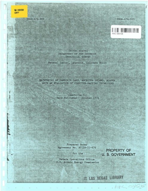
UNITED STATES
DEPARTMENT OF THE INTERIOR
GEOLOGICAL SURVEY
Faderal Center, Llcewood, Colorado 80225
BATHYMETRY OF CANNIKIN LAKE, AnCRITU ISLAND. ALASKA,
WITH AN EVALUATION OF COMPUTER MAPPING TECHNIQUES
Don Digeo GonerLee, Leonard E. Wollltz,
and G. E. Brerhauer

CONTENTS
Page
Abstract. . . . . . . . . . . . . . . . . .. . . . . . . , . . . . . 1
Introduction.............,........... ... 1
Acknowl.edgments . . . . . . . . . . . . . . . . . . . . . . . 5
Geologic and hydrologic setting . . . . . . . . . - . . . . . . . . 5
Effects of Cannikin . . . . . . . . . . . . . . . . . . . . . . . 6.
Bathymetry ...................... 8
Computerlnepping techniques . . . . . . . . . . . + . . . . . , . . 9
Comparison of computer-mapping techniques . . . . . . . . . . . . . 12
Computer calculation of cumuLarive volume . . . . . . . . . . . . . 15
Obliqueprojectiona . . . . . . . . . . . . . . . . . . . . . . . . 16
Smry ......................,.....,.16
References cited . . . . . . . . . . . . . . . . . . . . .. . . . . 20
ILLUSTRATIONS
Figure 1. Index map of report area showing location of
CannikinLake-. . . . . . . . . . . . . . . . . . . 2
2. Map showing primary geologic and hydrologic effects
resulting from the Cannikin event . . . . . . . . , . . 4
3. Manually-drawn bathymtric map and graph showing
stage-volume-area relation. of Cannikin Lake,
May 1973, Amchitka Island, AZaaka . . . . . . . . . [In pocket]
4. Computer-drawn bathymetric map of Cnnnikin Lake
ustug WET program, May 1973 . . . . . . . . . . . . 11

Figure 5. Computer-dram bathymetric map of Cannikin Lake,
Page
using Calcomp EPCP program, May 1973, Amchitka
Illand. Masks. .................. [Inpocket]
6. Oblique projection. Cannikin Lake, produced using
WET program ..................... 18
7. Oblique projection, with shaded relief, Cannikin Lake,
based on projection produced using WET program .... 19

This figure is not available in electronic format.
Please email lm.records@gjo.doe.gov to request the figure.

ABBIIEVIATIONS AND CONVERSION FACTORS
Multiply EnpLish Units & To Obtain Metric Units
Miles (mi) 1.609 Kilometres (km)
Feet (fe)
Inchem (in)
2
Square milre (aLt ) 2.590
0.3048 Metres (m)
0.0003048 KFleaetres (h)
2
Squrre kilometres (!a )
Acres 0.4047 Hectare8 (ha)
3
~cre-f ast (acre-f t 1 1233
Cubic metree (m
Miles per hour (ml/h) 0.868 Knote (k)
3
Cubic fear per second (ft /a) 0.02832 Cubic metres per second (m 3 1s)
r

UNITIDJ STATES
Amchitka-41 DEPARTMENT OF THE INTERIOR
1974 GEOLOGICAL SURVEY
Federal Center. Lakewood, Colorado 80225
BAT-RY OF CANNIKIN LAKE. MCHITKA ISLAND. AWLSKA.
WLTH AN EVALUATION OF COMPUTER-HAPPING TECEU?IQUES
Don Diago Gonzalez, Lebnard E. Wollitz. and G. E. Brethauer
ABSTRACT
Defining the ch.racteri8tics of Cannikin Lake was eaaential in
detedning the effect of a eubsurface nuclear detonation on the
hydrologic and biologic environment. A bathymtric mrp, the basic
geometry of the leke, and the stage-area-volume relationship were
derived from data produced by a sonic survey of the lake, At the
lake's highest level, the maximum dept is 31 feet (9.45 metres), it
h e a volume of 325 acre-feet (401 x l 3 cubic metres) and covers a
surface area of 30 acre. (12,1 hectares). A computer-mapping technique
utilizing two different computer programs OJET and Calcomp GPCP) was
used to evaluate the usefulness of the programs ae mapping tools. The
two bathymerric IMPS of the lake bottom produced by this method show
a high degree of reliability when compared with the hand-drawn version.
The Cannilcln event was detonated at a depth of 5,875 ft (1.79 km)
on Amchitka Island, Mask. (fig. l), on November 6, 1971. It was the
largest underground nuclear rest that the United States ham conducted,
Cannikin, with a yicZd of lees t hn 5 megatons, wus detonated in
saturated volcanic rock. MTlliseconds after the explosion the energy
of the device was expended, creathg a spherical cavity formed by
heat and pressure. The surrounding medium was fractured several

PACIFIC
OCEAN GROUND ZERO
&
2-
'"-c'
--d
AMCHIT KA ISLAND
ConniC/n Lokr
=RING
Figure I-- Index map of report area showing location of Cannikin Loke.
SEA
0 5 10 MILES
0 9 I0 KILOMETRES
u

cavity-radii from the point of the explosion. At the land surface, the
ground lifted and cracked from the force of the explosion {fig. 2).
Thirty-eight hours after the explosion, temperatures and pressures in
4
I
I
the underground cavity subaided sufficiently for the overlying rock to
collapee into the cavity. The collapee initiated the growth of a rubble I
chimney that extended to the land surface, forming a collapse stnk (ground
surface depreanion) with associated fractures and faults.
~
The daepeot part of the trianmlar colhpre sink warn offset about
1,500 ft (460 m) east of GZ (ground zero), the murface location of the I
~
8mpLacamnt hole. Thin topographic closure captured surface-water runoff
from 84 percent of the aurroundinng drainage aru (fig. 2). Stage recorders I
placed in the collapse mink Jn July 1972 nhowed that u lake began to form I
in August and began to rpill into the lower reaches of White Alice Creek
by December 1, 1972. Thim lake, commnly referred to as Cannlkin Luke by
the AEC (U.S. Atomic Energy Commission) md it8 contractors, was the first
lake created by an underground nuclear explomion.
The USGS (U.S. Geological Survey), in cooperation with the UC, has
the responsibility to docmnt and to interpret the geologic and hydrologic
effects of nuclear explosions. An accurate description of collapee @inks
is part of thie reaponoibility.
'
The formution of a hke within the collapne sink is a unique geologic
and hydrologic effect of an underground nuclear explosion. Cannikin LLae
ptwideo an opportunity to conduct bioenviro~wntul studies of a newlyformed
aquatic habitat and to determine dilution patterns in the event of I
radioactive lealuge. An accurate description of the lake bottom and I

volume of the lake, baaed on bathymetry, was necessary ro document and
interpret the geological, hydrological. and bioenvironmental effects
aseocinted with the creation of Cannikh Lake. r
The stage-volume relationohip for Cannikin Lake was calculated
' using the computer program. WET. This program and another, Calcomp
GFCP, were usad to produce bathymetclc maps from the same data.
Because the manually-drawn batbymetric map includes details determined
by photography and viaual observation before the lake basin wae aub-
merged, cornparimon of the maps provides a test of the reliability of
the computer program in mapping irregularly rpaced data.
Acknovled~nts
The authors wieh to express their gratitude to Wen Sammona of
Holmes and Narver, Inc., Las Vegas, Nevada, for his assistance in
making the murvey of Cannikin Lake.
GEOLOGIC AND HYDROLOGIC SETTING
The area surrounding Cannikin ground zero ranges in altitude from
50 ft (15.2 m) to 280 ft (85.3 m); the average altitude is 160 ft
(48.8 m). The land aurface is covered with turf and under1)ving peat
eu much as 13 ft (4 m ) thick. Bedrock consists predominately of
volcanic rocks, most of which were deposited under the sea 3r on the
flanks of volcanoem. The area drains northeastward toward rhe Bering
Sea. where the shoreline is characterized by steep cliffs ranging
from 40 to 60 ft (12.2 to 18.3 m) high.

The average annual precipitation is 30 to 35 in (762 to 889 m)
including an average snowfall of 70 in (1,778 nun). Wind velocities
sometimes exceed 100 mi/h (87 k) in the winter, and average 20 to 25 mi/h
(17 to 22 k) during the summer months. The drainage area surrounding GZ
2 2
is 0.80 mi (2.07 h ) and Xe drained by White Alice Creek, which flows
northeaetward to the Bering Sea (fig. 2). Streamflow records collected
near the muth between August 1968 and November 1971 indicate that the
3
mean average flow in White Alice Creek was appr~htely 2.80 ft /e
3 3 3
(0.08 m /a). This flow, approximrtely 2,000 acre-ft (2,470 x 10 m )
per year, is expected to be the approximate annual drainage into
Cannikin Lake after equilibrim 16 established.
EFFECTS OF CANNXUN
At the time of the detonation numerous fracture. md faults were
created; one major northwesterly fault occurred perpendicular to the
south fork of White Alice Creek. The upthrown block of this fault
immediately prevented norm1 runoff and water began to collect on the
downthrowl aide of the fault, fodng a pond (hatched area within Cannikin
Lake on figure 2). Cavity collapme occurred 38 hours after the detona-
tion, and reaulted in a triangular ground-murface depression. Pertinent
features of the collapse were major faults that trend east-northeast,
north, and weer-northwest (fig. 2). Dnly the rmjor faults and thoue
significant to the form~tion of Cannikin Lake are shown on figure 2.
For a more detailed discussion of the structural. geology refer to Morris
and Snyder, 1972. Recent surveys by the U.S. Geological Survey and by
Holmea and Narver, Inc. indicate tbt the maximum subsidence is about

.-
Following the detonation and collapse, the drainage area surrounding
GZ (fig. 2) was severely altered by upheaval, compressional forces, and
. major faulting (Gonzalez and Wollitz, 1972). Eighty-four percent of the
original drainage area warn temporarily rransfonned into a closed bsain,
the lowermoat part of which contain8 Cannikin Lake. This basin, the
area west of the dotted Line doithin the drainage boundary on figure 2,
comprises 425 acres (172 ha) of which 30 acres (12.1 ha) was covered by
the lake at ita highest known elevation. Water in the Lake is main.niy
surface-water runoff frmn the upper reaches of White Mice Creek and
seepage from the shallow water table.
The apillway of Cannikin Lake is formed by an eastnortheast-
trending fault where it intersects the north fork of White Alice Creek
(fig. 2). This fault, which occurred at the time of collapse, had a
vertical displacement of LO ft (3.05 m) and a right-lateral horizontal
diaplacement of 2 ft (0.61 m). At the higheat h o w Level of 116 ft
(35.4 m) above msl, the lake covered 30 rcres (12.1 h.) and stored
3 3
325 acre-ft (401 x 10 m ) of water. The lake begm,to spill into the
main reach of White Alice Creek 78 days after puddles began to stare
water in the low sreae of the depreseion, indicating saturation of the
underlying materials in the rubble chihimney. The elsv~tion of the
spillway is estimated at 134 ft (34.7 m) above m l, while the lowest
elevation in the lake determined by mounding is about 85 fr (25.9 m)
above mal. The lake is about 2.150 ft (655 m) long. has an average
width of 650 it (198 m), md has 1.3 mi (2,09 h) of shoreline.

.>
BATHYMETRY
The bathymetric map of Cannikin Lake is based on a sonic and land
survey made in May 1973. Horizontal control consisted of a closed survey
made around the lake. Control points were aligned at traverse statfons
using a transit positioned on a temporary benchmark. Right angle8 were
turned with a compass and distances were measured with a surveying chain.
The survey wan adjusted one-half degree for closure between two permanent
benchmark*.
Boat traverses with a sonic sounder were made acronr the width and
length of the lake. Traverses were controlled and positions were determined
by line of sight uning Lath at a traverme station as a control point.
Weather conditiunm during the survey were exceptionally good. Ten traverses
were made the width of the lake and four traverses the length of the lake.
Vertical control (edge of water), established by differential levels
from poet-detonation ground-zero conrrol, was determined to be 114.8 ft
(35.0'm) above ml at the time of the Purvey.
Vertical eoundings from the eonic sounder were recorded on a contin-
uoua strip-chart recorder; the eoundings are accurate to the nearest tenth
of a foot. The number of data pointa selected along each traverae were
based on change in relief on the lake bottom. From these traverses,
760 data points were used for anrlymis.
The m~nually-drawn bethymetric map (fig. 3) was based on data from
the sonic survey and knowledge of the bamin before it filled with water.
The contour intervilis 2 ft (0.611~). Most of the steep slopes shown by
close mpacing of the contourm indicate faulting.
r

Stage-area-volume relacionships were calculared from the baafc dara.
and the water-surface areas for different lake levels were measured using
standard planimetric techniques. The manually-drawn map as well as the
computer versions were ueed to obtain these relationehips. The two net6
of results are similar; they are shown on figure 3.
COMPUTER-MAPPING TECHNIQUES
The traverse dara obtained from the bothymetric survey of Cannikin
take gave the authors an opportunity to rest the applicabitity of current
computer-mapping techniqueu for traverse-type data. Bathymetric maps were
produced using two different computer program (WET and Calcomp EPCP) and
were compared with a manually-drawn bathymctric map. In addition to the
bathjrmetric mpe, part of the WET computer program was used to produce an
oblique three-dimeneional projection of the lake bruin, and to calculate
the volume of water in the lake at given water lsvsls.
There are three distinct uteps in computerized map production:
1. Data Preparation. Entablish an x-y coordinate system whose
orientation and acale are compatible with the size and shape of the lake.
The x and y coordinate of the data point and the measured -ake-bottom
elevation at that point are coded and then key-punched on computer cards.
2. Data Conversion. The data from step L are used as input into a
computer program which calculstea lab-bottw altitudes for an array of
regularly-spaced points covering the entire area of the lake.
3. Manipulation of Converted Data. This array of x-y coordinates
and calculated lake-bottom altitudes is used as input to one ir both of
the computer programs. Each of the computer progrme is used to produce
planimetric maps of the lake-bottom altitude*. Appropriate parts of the
9

WET computer program ate selecced ro produce oblique three-dirnens;loea1
projections, and to calculate the volume of water in rhe lake at given
water levels.
The parameters used in 8teps 2 and 3 that influence the quality of
contour and oblique projection8 and volumetric calculations are grid size,
map scale, contour interval, and tho x, y, and z coordi~tes of obsewarion
points used in the production of oblique projections. The values of theee
parameter8 are baaed on the type of basic data being inve&t:gated (clustered,
sparse, Linear, etc.), the change in the calculared lake-bottom altitude
values, specific control required, and directions and areas of interest.
The WET Nahl-Evenden-Van Trump) program was written and (or) modified
by R. R. Uahl, G. I. Evenden. and George Van Trump, Jr. of the U.S. Geological
Survey. The program is designed to calculate surface values at grid inter-
sections of a regularly-.paced grid using surface value. at irregularly-
apaced pointo as input. The interpretative portion of this program emplaya
a locally-weighted, leaat-square. surface-fitting technique. This program
is designed to allow the user the option of using the output tape to
produce a bathmetric mpp (fig. 4) or an oblique projection of the surface.
The part of the program used to obtain the oblique projections is based on
work by Wright (1973) and wan modified for use on the IBM 360-65.
The Calcomp GPCP (Calcomp, 1971) program is available ior users of
the U.S. Geological Survey IBM 360-65 computer system. This progranl also
celculates surface values at grid intersections of a regularly-apaced grid
using surface values at irregularly-.paced points &e input. The fnterpreta-
tive part differ. from the WET program and consists of two operations. The

Universal Transverse Mcrcotor Proiection IUTMI
400-foot grid tick, zone 60
m FEET
rnelres) above mean sea lNel
Figure 4-- Computer-drawn bat hymetric map of Cannikin Lake, using WET program, May 1973

....
firer operation determinee the gradient or rangenr-plane ar: each date point
using a specified number of neighboring points. This plane must pass
through the z value of the datum point in quemtion and the angles this
plane makes with vectors to the specified neighboring points are minimfeed.
The second operation uaea the gradients at a specified number of data points
and a weighting function to determine the surface values at the grid inter-
sections of a regularly-spaced grid. The number of neighboring points uaed
r
in each operation (neighborhood) and the size of che grid are specified by L
the user. The map made using the Calcomp GPCP program is shown on figure 5.
COMPARISON OF COMPUTER-WP'ING TECHNIQUES
The same baaic data were used in production of all bathymetric mapa
except that subjective control was used in the enuaLly-dram map based on
terrain knowledge obtained before and after the lake started to fill with
water, For this reason the manually-drawn version is probably more realistic
and waa nelected as the basis of comparison. In general, the computer-
produced mapa showed a definite similarity to the manually-dram map.
The degree of similarity between the computer mapc ind rhe manually-
drawn map was directly related to the selection of grid size and neighbor-
hood, Varying the grid mize and deighborhood during trhl runs of the WET
and Calcomp GPCP programs ahowed the followfng:
1. Features would not appear unleas the grid sXze was approximately
one-half (or lean) of the minimum diameter of the feature;
2. Small grid sizes tend to break up and localize long linear
features; and
3. Large neighborhoods should be used with traverse-type data. as
is done in this report.
12
r
p

The water-level datum used for both computer programs iu 114.8 ft (35.0 m) ~
above msl, while that of the manually-drawn version is rounded to 115 ft
(35.0 m) above msl. The computer-drawn msps were plotted at 3-ft (0.30-m)
intervale; therefore, the highest altitude contour shown on the computer
maps is lL4 ft (34.75 m). This contour line was used as the shoreline
datum for both computer-produced maps. This difference in shoreline datum
remults in a slightly larger surface area on the mually-drawn map and I
makes the depths 1 f t (0.30 m) greater. I
The map produced by the WET program (fig. 4), when compared with the
manually-drawn map, matches the outline of the laks~hore very closely
(fig. 3); however, the match between contours of the two maps i& less
exact. The low areas are in about the correct pernpective but the mounds
are nearly all omitted. I
The Calcomp GPCP product (fig. 5) is a very close approximation of
the hand-drawn veroion. Difference. in shoreline configuration may be
a result of several. factors. 1
In relief.
1. A difference in ehoreline datum;
2. A mnoothing property inherent in both computer programs; and
3, An inadequate shoreline control where there is a rapid change
At the southwest end of the lake, only local detaile are omitted-- I
that is, two mounds and a shallow depression; however, the main featurea
are apparent. Theme are the outline of the pond formed by the northweat-
trending fault and its outlet. Water depths are consistent with figure 3. I
r
!

The middle part of the lake also lacks some of the local details
but the main featurea are present. The Calcomp GPCP program has not
. completely iaolated the actual mounds end depreeaionm but has characterized r
them a. knolls or fingers. isolation of theae mound8 could probably be
effected by slightly decreasing the grid nize. The deeper parts of the
lake conform well to the manually-drawn version.
The northeast part of the lake show the poorest correlation, because
of the omission of a depreanion and a weak impression of the uppermost mound.
In this region, where there i m rapid chunge In altitude, the poor correlation
may be due to inadequate shoreline control. This tende to centralize the
deeper areas rather than offnet them as in the manually-drawn map.
As a whole, the cornparibon is good and gives a good repreeentation of
the main features shown in the manually-drawn map. Some of the local
features omitted on the map produced using the Calcomp GPCP program could
be brought out by decreaming the grid size; hawever, too small a grid size
will tend to break up the long linerr featurea shown which correlate well
with the name features on the manually-drawn map.
The map produced using the Calcomp GPCP program compared more favorably
with the manually-drawn map than did the mrp produced using the WET program.
The map produced using the Calcomp GPCP program permitted recognition of
smaller features withour breaking up the long linear features when using
the same grid size for both programs.
14
US. D.O.L.
D ~ I N TECHN~CAL V
INFOF~T~AYION
~ R ( X . G E ~
P'
L
.
.F

COMPUIXR CALCULATION OF CUMWIATIVE VOLUME
A plot tape produced ueing the WET program contained an array of
values giving the x and y coordLnates and the calculated elevation of the
lake bottom at regularly-spaced distances over an area covering the entire
lab. This array was used to calculate the volume of water in the lake
for any desired water elevation uming the following procedure:
Plot the array of x and y coordinates covering the lake. The distance
between two adjacent pointm with the same y coordinate is Ax. The distance
between two adjacent pointa with the same x coordinate in Ay. In the WET
program. Ax and Ay were equal, thus the distance between parallel x or y
coordinates i8 equal and is called Ad.
As 8tated previously, a calculated altitude of the lake bottom is
associated with each point (x and y coordinate). Aaaume that thin altitude
L
is constant for a square of area ( hd) in which the point (x,y coordinate)
is located at the center of the square. The volume of the lake can be
calculated by subtracting the calcuhtcd altitude of the lake bottom at
each applicable point from the given water-level altitude, multiplying
this difference by ( ~d)*, and su~ng this remult for all applicable
points. An applicable point would be we for which the calculated altitude
of the Lake bottom wan lower than the given water-lmel altitude.
The array from the WET program plot tape was read in as input to part
of the WET computer program which scanned the calculated altitude values of
the lake bottom and noted and stored each different altitude value. These
altitude values were then sorted in ascending order and used as given water-
level altitudes to calculate the volume of the lake using the method described
above. These water-level altitudes versus volumetric results are shown as
the stagevolume relationehip for Cannikfn Lake in figure 3.
15
-
-

OBLIQUE PROJECTIONS
The result of using the oblique-projection option in the WET
program is shown in figure 6 and is typical of the type of representations
produced. The oblique projections of the lake bottom are viewed downstream
toward the intersection of the northeast-trending fault and White Alice
Creek. Variations in perspective may be obtained by varying the x-y-z
vfewing coordinates. A pictorial view may be obtained and St is possible
co produce views of the lake bottom as would be seen from above or below
shoreline datum by using various shading techniques as those shown on
figure 7. These figures are often helpful in visualizing features
displayed on the computer-produced plarrimetric contour maps. A change
in the viewing position allowe one to view certain pertinent feature6
along a favorable line of sight.
SIMMARY
The detonation of the Cannikin nuclear explosion and subaequent
collapee in the area has created Amchitka's most outstanding lake. The
manually-drawn bathymetric map (fig. 3), based on data from a monic survey
made of the lake, is the standard of comparison for two additional bathy-
metric maps produced from two computer-mapping programs using the same
data. These are the WET program and the Calcomp GPCP program. The com-
parisons show tht the Calcomp program, with proper selection of neighbor-
hood and grid uize, can produce a map that compares very well with the
hand-drawn standard.
-
\

The WET program gives a clone approximation of the standard baais
and is a fair representation. ELeny of the local effects are omitted and
the features are generalized.
A table sunrmarizing the characteristics of Cannikin Lake is pre-
nented on figure 3.

Figure 6-- Oblique projection, Connikin Lake,produced using WET program.
18

Figure 7:-Oblique projections,, with shaded relief, Cannikin Lake, based on
projection produced using WET program.

REFERENCES CITED
Calcomp, 1971, A general purpose contouring program, users manual:
California Cornpurer Products. Znc., 2411 W. La Palma Ave.,
Anaheim, CA 92801.
Gonzelez, D. D.,. and WolLitz, L. E., 1972, Rydrologic effects of the
Cannikh event, &Geologic and hydrologic effects of the Cannikin
underground nuclear exploeion, AmchitkP Inland, Alaaka: U.S. Geol.
Survey rept. USGS-474-148, p. 39-67; available from U.S. Dept.
Comerce, Natl. Tech. Inf. Service, Springfield, VA 22151.
Morris, R. H., and Snyder, R. P., 1972, Vinible geologic effects,
Geologic and hydrologic effects of the h ikin underground nuclear
explosion. Amchitka IsSand, Alaska: U.S. Geol. Survey rept.
USGS-474-148, p. 5-17; available &from U.S. Dept. Commerce,
Natl. Tech. Inf. Service. Springfield, VA 22151.
Wright, T. J., 1973, A two npace solution to the hidden line problem
for plotting functions of tuu variablen: IEEE Trans. on Computers,
v. C-22, no. 1, p. 28-33.

I
U.S. Atomic Energy Codssion. Nevada Operations Office, Las Vefies, Nevada: !
E. M. Douthett (3)
M. E. Gates, c/o R. R. LOU (2)
D. M. Hamel (3)
D. G. Jackson (3)
R. B. Loux (20)
Roger Ray
R. H. Thalgott
A. J. Whirman
U.S. Atomic Energy Co@ssion, Nevada Test Sire Support Office,
Mercury. Nevada :
U.S. Atomic Energy Cmssion. Mercury. Nevadr:
CETO Library
U.S. Atomic Energy Commission, Washington, D.C.:
M. B. Biles (2)
Ernest Graves
J. A. Harris, Jr.
G. W. Johnson
. L. Livemn
W. H. Pennington
U.S. Atomic Energy Commission; Technical Znformrtion Center.
Oak Ridge, Tennessee: (2)
Defense Nuclear &ency:
Comnder, Field C-d (Attn: Benjarin Grote).
Kirtland AFB, Nev Mexico
Director (Attn: SPSS, John Lewis. Clifton MacFarland).
Washington, D.C+
0-I-C Liaieon Office, La6 Vegas, Nevada

Loa 4lamos Scientific Laboratory, Lon Alamoa, New Mexico:
Robert Bradshaw
C. I. Brme
R. B. BrownLee
E. A. Bryant
R. H. Campbell
R. R. Sharp, Jr.
Lawrence Livermore Laboratory. Livermore, Califomin:
R. E. Batzel
J. E. Carothers
P. E. CoyLe
D. 0. Emerson
L. S. Germain
Alfred Holzer
A. E. Lewis
L. D. Ramport
H. C. Rodean
W. L Sprin~er
Technical Information Divimion
G. C. Werth
Lawrence Livennore Laboratory. Mercury. Nevade:
W. B. McKinnio
Sandie Laboratories, Albuquerque. Ntw Mexico:
J. R. Banister
C. D. Broyles
M. L. Merritt
W. C. VoLlendorf
W. D. Wearr
WOO Panel of Conrultants:
Joseph Linrz. University of Nevada, Rmo, Nevnda
N. M. Newmark, University of fllinois, Urbarra. Illjnoie
T. F. Thompson, 2845 Rivera Drive, Burlingme, California
S. I). Wilaon, Shannon & Wilson, Inc., Seattle. Washington
P. A. Witherspoon, University of California, Berkeley, California
Advanced Research Project. Agency. Arlington. Virginia:
S. J. Lukasik

.- Battells CoLumbus Laboratories:
R. S. Davidson, CoLumbus, Ohio
V. Q. Hale, Las Vegas. Nevada
3. B. Xirkwood, Duxbury, Maasachuaetts
CIRES. University of Colorado. Boulder, Colorado:
E. R. Engdahl.
Desert Research Institute. Reno. Nevada:
Environmental Protection Agency:
Atm: Water Branch, Seattle, Wamhington
Environmental Protection Agency. National Enviro-tal Rebearch
Center. h a Vegas. Nevada:
D. S. Barrh
Fenh & Scisson, Inc.:
Grant Bruesch, Mercury. Nevada
M. H. May. Lee Vegre. Nevada
Holmes & Narver. Inc.. Las Veaas. Nevada:
F. M. Drake
National Oceanic and Atmosvheric &inistrrtion, Air Resources
Laboratory. Las Vegas. Nevada:
National Oceanic and Atmos~hrric Admillistrrtion, National Marine
Fisheries Service. Auke Bay. Alaska:
T, R. Merrell, Jr.
University of Washinxton. Scuttle. Washington:

.-
*
U.S. Army Corpe of En~ineers, Alaska District. Anchorage, Alaska:
District Engineer. Attn: A. C. Marhewa
U.S. Army Corps of Engineer.. Waterways Exueriment Station,
Vicksburx. Ellssiesifi:
Library
U.S. Bureau of Mines. Denver. Colorado:
U.S. Department of Interior. Bureau of Sport Fimhtries and Wildlife.
Anchorage, Alaska:
C. E. Abegglen
U.S. Geological Survel:
Geologic Data Center. Mercury, Nevada (15)
K. W. Ring, Las Vegas, Nevada
Library, Denver, Colorado
Library, Menlo Park, Cllif ornia
Don Tocher. Menlo Park. CaLifomia
U.S. EeoJo~ical Survey. Remton. Vir&d.a:
Chief Hydrologist, WRD (Attn: Radiohydrology Section)
Library
Militnry Geology Unit
J. C. Reed, Jr.