The Birth of Insurance Contracts - The Ataturk Institute for Modern ...
The Birth of Insurance Contracts - The Ataturk Institute for Modern ...
The Birth of Insurance Contracts - The Ataturk Institute for Modern ...

You also want an ePaper? Increase the reach of your titles
YUMPU automatically turns print PDFs into web optimized ePapers that Google loves.
1 Introduction<br />
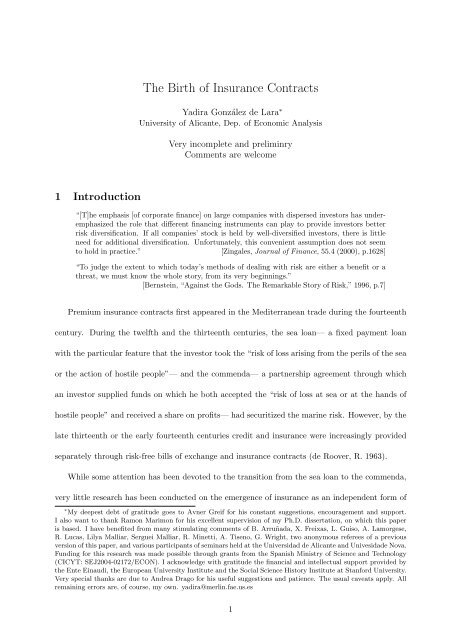
<strong>The</strong> <strong>Birth</strong> <strong>of</strong> <strong>Insurance</strong> <strong>Contracts</strong><br />
Yadira González de Lara ∗<br />
University <strong>of</strong> Alicante, Dep. <strong>of</strong> Economic Analysis<br />
Very incomplete and preliminry<br />
Comments are welcome<br />
“[T]he emphasis [<strong>of</strong> corporate finance] on large companies with dispersed investors has underemphasized<br />
the role that different financing instruments can play to provide investors better<br />
risk diversification. If all companies’ stock is held by well-diversified investors, there is little<br />
need <strong>for</strong> additional diversification. Un<strong>for</strong>tunately, this convenient assumption does not seem<br />
to hold in practice.” [Zingales, Journal <strong>of</strong> Finance, 55.4 (2000), p.1628]<br />
“To judge the extent to which today’s methods <strong>of</strong> dealing with risk are either a benefit or a<br />
threat, we must know the whole story, from its very beginnings.”<br />
[Bernstein, “Against the Gods. <strong>The</strong> Remarkable Story <strong>of</strong> Risk,” 1996, p.7]<br />
Premium insurance contracts first appeared in the Mediterranean trade during the fourteenth<br />
century. During the twelfth and the thirteenth centuries, the sea loan— a fixed payment loan<br />
with the particular feature that the investor took the “risk <strong>of</strong> loss arising from the perils <strong>of</strong> the sea<br />
or the action <strong>of</strong> hostile people”— and the commenda— a partnership agreement through which<br />
an investor supplied funds on which he both accepted the “risk <strong>of</strong> loss at sea or at the hands <strong>of</strong><br />
hostile people” and received a share on pr<strong>of</strong>its— had securitized the marine risk. However, by the<br />
late thirteenth or the early fourteenth centuries credit and insurance were increasingly provided<br />
separately through risk-free bills <strong>of</strong> exchange and insurance contracts (de Roover, R. 1963).<br />
While some attention has been devoted to the transition from the sea loan to the commenda,<br />
very little research has been conducted on the emergence <strong>of</strong> insurance as an independent <strong>for</strong>m <strong>of</strong><br />
∗ My deepest debt <strong>of</strong> gratitude goes to Avner Greif <strong>for</strong> his constant suggestions, encouragement and support.<br />
I also want to thank Ramon Marimon <strong>for</strong> his excellent supervision <strong>of</strong> my Ph.D. dissertation, on which this paper<br />
is based. I have benefited from many stimulating comments <strong>of</strong> B. Arruñada, X. Freixas, L. Guiso, A. Lamorgese,<br />
R. Lucas, Lilya Malliar, Serguei Malliar, R. Minetti, A. Tiseno, G. Wright, two anonymous referees <strong>of</strong> a previous<br />
version <strong>of</strong> this paper, and various participants <strong>of</strong> seminars held at the Universidad de Alicante and Univesidade Nova.<br />
Funding <strong>for</strong> this research was made possible through grants from the Spanish Ministry <strong>of</strong> Science and Technology<br />
(CICYT: SEJ2004-02172/ECON). I acknowledge with gratitude the financial and intellectual support provided by<br />
the Ente Einaudi, the European University <strong>Institute</strong> and the Social Science History <strong>Institute</strong> at Stan<strong>for</strong>d University.<br />
Very special thanks are due to Andrea Drago <strong>for</strong> his useful suggestions and patience. <strong>The</strong> usual caveats apply. All<br />
remaining errors are, <strong>of</strong> course, my own. yadira@merlin.fae.us.es<br />
1
usiness. Economic historians have noted the advantage <strong>of</strong> the commenda over the sea loan in<br />
terms <strong>of</strong> risk-sharing (Lane, 1966, pp.61-63, and Lopez, 1952, pp.76 and 104) and have associated<br />
the introduction <strong>of</strong> premium insurance both with the increased use <strong>of</strong> the bill <strong>of</strong> exchange <strong>for</strong><br />
the financing <strong>of</strong> overseas trade and with the organization <strong>of</strong> this trade by means <strong>of</strong> permanent<br />
representatives abroad (de Roover, F.E., 1945, pp. 173 and 177). Yet, no satisfactory explanation<br />
<strong>for</strong> the observed selection <strong>of</strong> contracts have been so far provided.<br />
As the sea loan and the commenda resemble today’s debt and equity contracts, on the one<br />
hand, and fix-rental and sharecropping agreements, on the other hand, modern economic theory<br />
might shed light on their use. 1 Contrary to the Corporate Finance literature, Transaction<br />
Costs Economics, and the Historical Institutional Analysis, this paper, however, ignores the role<br />
<strong>of</strong> verification/falsification costs, multiple margins <strong>for</strong> moral hazard, adverse selection, signaling,<br />
incomplete contracting, transaction costs, and institutions <strong>for</strong> contract en<strong>for</strong>cement in shaping<br />
contracts. 2 Instead the choice between the sea loan or the commenda derives from simple,<br />
although historically backed, in<strong>for</strong>mation assumptions: under hidden in<strong>for</strong>mation, the sea loan<br />
emerges as a second-best because contracts cannot be contingent <strong>of</strong> the venture’s commercial<br />
pr<strong>of</strong>it; under full in<strong>for</strong>mation, incentive-compatible constraints are relaxed, enabling the adoption<br />
<strong>of</strong> the first-best better risk-sharing commenda (Townsend, 1982).<br />
<strong>The</strong> paper, on the contrary, focuses on the role that different financial instruments play to<br />
provide the optimal allocation <strong>of</strong> risk, in particular, <strong>of</strong> marine risk. Like today’s debt and equity<br />
contracts, the sea loan and the commenda provided limited liability to both the merchant, who<br />
was exempted from repayment beyond the venture’s assets in case <strong>of</strong> loss at sea or at the hands<br />
1 <strong>The</strong> sea loan and the commenda indeed served the double function <strong>of</strong> financing and organizing overseas trade<br />
using someone else’s capital. In Venice, <strong>for</strong> example, both types <strong>of</strong> contract worked as financial instruments through<br />
which business capital together with personal savings, small incomes and legacies were mobilized into risky investments<br />
in overseas trade (Lane, 1973, and González de Lara, 2005). In twelfth-century Genoa, however, the<br />
commenda operated mostly as a labor contract to handle the investor’s business abroad (Greif, 1989 and 1993).<br />
Accordingly, the investing party have been referred to in the literature as sleeping partner, stay at home or<br />
sedentary merchant, principal, stans, and commendator. Similarly, the travelling merchant has been called managing<br />
partner, carrier, factor or agent, tractans or procertans, and accomendatarius. Since this paper focuses on the marine<br />
risk allocation that different contracts entailed, I shall use the terms “financier” and ”merchant.”<br />
2 <strong>The</strong> companion piece <strong>of</strong> this paper analyzes the en<strong>for</strong>cement and in<strong>for</strong>mation problems underlying the transition<br />
from the sea loan to the commenda in late-medieval Venice and finds that, in this particular episode, institutional<br />
developments that enhanced the state’s ability to verify in<strong>for</strong>mation enabled the adoption <strong>of</strong> the better risk-sharing<br />
commenda. EXPLAIN<br />
2
<strong>of</strong> hostile people, and to the investor, who risked loosing only the capital advanced. Commonly,<br />
merchants received funds from several financiers, while investing in other merchants’ ventures <strong>for</strong><br />
the sake <strong>of</strong> diversification. Optimal Portfolio Selection theory can account <strong>for</strong> the merchant’s<br />
reliance on external funds on the basis <strong>of</strong> managerial risk aversion, but takes the specific <strong>for</strong>m <strong>of</strong><br />
contracts (securities) under which funds are raised as exogenously given. <strong>The</strong> Optimal Security<br />
Design literature derives endogenously the characteristics <strong>of</strong> debt and equity under the assumption<br />
that all contracting parties are risk neutral, but predicts the maximum investment participation<br />
<strong>of</strong> the merchant to the venture (<strong>for</strong> excellent surveys <strong>of</strong> Corporate Finance, see Harris and Raviv,<br />
1991, and Zingales, 2000). 3 However, the evidence indicates that medieval merchants both were<br />
risk averse and resorted to external funds be<strong>for</strong>e investing 100 percent <strong>of</strong> their own wealth in<br />
the sea venture they manage. 4 More importantly, neither the Traditional Capital-Structure<br />
theories nor the the Optimal Security Design literature have addressed the evolution from the<br />
securitization <strong>of</strong> the marine risk through debt-like sea loans and equity-like commenda contracts<br />
to the provision <strong>of</strong> insurance, not through the capital market, but through premium policies.<br />
<strong>The</strong> sea loan and the commenda differed from a combination <strong>of</strong> premium insurance and a<br />
risk-free bill <strong>of</strong> exchange in two respects. First, both the sea loan and the commenda conferred<br />
the merchant less protection against the marine risk than pure insurance contracts, which did not<br />
only exempt the merchant from repayment beyond what was saved from mis<strong>for</strong>tune at sea but<br />
also provided a coverage payment to <strong>of</strong>fset the merchant’s lack <strong>of</strong> gain in the event <strong>of</strong> a marine<br />
incident. Second, whereas the sea loan and the commenda exchanged funds <strong>for</strong> a claim on the<br />
venture’s returns, both the bill <strong>of</strong> exchange and the pure insurance contract established payments<br />
from the agents’ personal wealth. Historical evidence suggests that en<strong>for</strong>cing these payments was<br />
more difficult and costly than ensuring that the investor received a fair return from the venture.<br />
<strong>The</strong> paper proposes a historically-grounded mechanism-design model <strong>of</strong> corporate finance with<br />
3 <strong>The</strong> Costly State-Verification literatures explicitly recognized that standard debt contracts are not efficient if<br />
the parties are risk averse (Townsend, 1978, p. ?, and Gale and Hellwig, 1981, p. ?). Under risk-neutrality, contracts<br />
are optimally designed to minimize in<strong>for</strong>mation and/or transaction costs. <strong>The</strong>re<strong>for</strong>e, the best a merchant can do<br />
is to finance the project he manages in its entirety, unless restricted to rely on external funds because <strong>of</strong> budget<br />
constraints and hence the prediction <strong>of</strong> a maximum inside participation rate to the firms’ investments.<br />
4 Zingales (2000) and (1995, table IV, p. 1439) provides equivalent evidence on today’s entrepreneurs/firms.<br />
3
two-side risk aversion and costly contract en<strong>for</strong>cement where the optimal contract choice depends<br />
on the risk and cost <strong>of</strong> a non-diversifiable investment project. In particular, if the project is highly<br />
risky and costly, the optimal risk allocation can be achieved either through letting the merchant<br />
finance a part <strong>of</strong> the venture and raising the remaining capital through a limited-liability sea loan<br />
or a commenda contract or through a combination <strong>of</strong> a risk-free bill <strong>of</strong> exchange and an insurance<br />
policy. Yet, the <strong>for</strong>mer is Pareto superior under the assumption that the agents’ personal wealth<br />
is contractible at a higher en<strong>for</strong>cement cost than the project’s returns (when the merchant lacks<br />
enough wealth to finance the project himself and/or collateral to repay in full in case <strong>of</strong> loss,<br />
the sea loan or the commenda uniquely sustains the optimal allocation <strong>of</strong> risk). However, if the<br />
project is relatively less risky and costly, the optimal risk allocation calls <strong>for</strong> more insurance than<br />
what limited-liability sea loans and commenda contracts provide to the merchant, thereby making<br />
insurance policies unavoidable.<br />
Consistent with the model’s predictions, we observe that the sea loan and the commenda<br />
actually gave way to marine insurance when commerce lost many <strong>of</strong> its adventurous features and<br />
wealth accumulation from commerce reduced the <strong>for</strong>mer scarcity <strong>of</strong> capital (Lopez, 1976, p. 97).<br />
<strong>The</strong> organization <strong>of</strong> the paper is as follows. Section 2 sets and solves the model, while sections<br />
3 evaluates empirically the assumptions and predictions <strong>of</strong> the model. Finally, section 4 concludes.<br />
2 <strong>The</strong> Model<br />
Consider a one-period two-dates contracting economy with a merchant and a financier who face<br />
the possibility to undertake a single welfare-enhancing trading venture. Both agents are risk<br />
averse with preferences represented by continuous and twice-differentiable utility functions Ui(ci)<br />
exhibiting a decreasing absolute risk aversion (DARA) coefficient with U ′ i<br />
(.) > 0, U ′′<br />
i (.) < 0,<br />
where c denotes consumption and the subscript i = 1, 2 stands <strong>for</strong> the merchant and the financier,<br />
respectively. 5 Each agent i is initially endowed with ki units <strong>of</strong> good and maximizes his expected<br />
5 Note that Innada conditions are not assumed to hold, so that we do not <strong>for</strong>ce an interior solution.<br />
4
utility from second-date consumption. Goods can be costlessly self-stored or invested in the<br />
trading venture. Any amount <strong>of</strong> the good can be stored but the investment is lumpy. <strong>The</strong> venture<br />
requires k units <strong>of</strong> investment, plus the entrepreneurship <strong>of</strong> the merchant. It yields a random<br />
return s ∈ S = {y, x, ¯x} with probability ps, where y denotes the loss due to the marine risk<br />
and {x, ¯x} stand <strong>for</strong> the risky commercial return, with 0 ≤ y ≪ k ≪ x < ¯x and k < E[s].<br />
<strong>The</strong> marine risk refers to the so-called “risk <strong>of</strong> sea and people” and includes the risk <strong>of</strong> natural<br />
shipwreck, piracy and confiscation <strong>of</strong> property by <strong>for</strong>eign rulers. <strong>The</strong> commercial risk accounts <strong>for</strong><br />
wide variations in pr<strong>of</strong>its depending on the tariffs and bribes paid in customs, transportation and<br />
storage fees, the conditions <strong>of</strong> the goods upon arrival after hazardous trips, fluctuations in prices,<br />
and so on and so <strong>for</strong>th.<br />
To account <strong>for</strong> the optimality <strong>of</strong> undertaking the investment project we assume that<br />
E[Ui(s)] > Ui(k) ∀i, (1)<br />
which in combination with DARA ensures that the higher productivity <strong>of</strong> the trading venture<br />
(E[s] > k) compensates <strong>for</strong> its risk. <strong>The</strong>re<strong>for</strong>e, agents will only self-store and consume their<br />
autarkic endowments, ki, if they are unable to mobilize funds in long-distance trade. For ease <strong>of</strong><br />
notation, let w(s) = k1 + k2 − k + s be the second-date total risky endowment <strong>of</strong> the economy<br />
when the venture is undertaken. We first study the case in which the merchant is constrained to<br />
rely on external funds because <strong>of</strong> budget constraints and, <strong>for</strong> simplicity, he is assumed to have<br />
zero initial wealth, k1 = 0. <strong>The</strong>n, the model is extended to capture the situation in which the<br />
merchant can finance the venture entirely on his own, k1 > k. <strong>The</strong> financier is always endowed<br />
with enough resources to fund the venture, k2 > k.<br />
To keep the structure as simple as possible, the model assumes that the legal system can en<strong>for</strong>ce<br />
contracts contingent on verifiable in<strong>for</strong>mation at no cost, although this unrealistic assumption<br />
is relaxed in section 3.2. At the first date, when investment decisions are taken, there is no<br />
in<strong>for</strong>mation whatsoever on the true realization <strong>of</strong> the venture return. At the second date the<br />
return is realized and revealed to the merchant. While losses “at sea or from the action <strong>of</strong><br />
5
enemies” are assumed to be verifiable, the model considers two extreme scenarios regarding the<br />
ability <strong>of</strong> the State to verify the commercial return. Under hidden in<strong>for</strong>mation the commercial<br />
returns is non-verifiable, at any cost, but the State can <strong>for</strong>ce the merchant pay out the minimum<br />
possible commercial return, x. Under the full in<strong>for</strong>mation structure the commercial return is<br />
verifiable without any private cost <strong>for</strong> the financier.<br />
2.1 <strong>Contracts</strong><br />
We consider allocations that can be obtained by means <strong>of</strong> a contract enabling the funding <strong>of</strong><br />
the venture and specifying transfers from the merchant to the financier both at the first and<br />
at the second date. Whereas first-date transfers τ ∈ ℜ are prior to the realization <strong>of</strong> the state<br />
and, accordingly, are independent <strong>of</strong> it, second-date transfers τ(s) are contingent on the state.<br />
A contract will result in consumption schedules <strong>for</strong> the merchant and the financier, c1 and c2<br />
respectively, where c1 := c1(s) = k1 − k + s − [τ + τ(s)] and c2 := c2(s) = k2 + [τ + τ(s)]. 6<br />
Sometimes the merchant lacked the capital required to undertake a sea venture. Others,<br />
however, he was a man <strong>of</strong> substance who could fund the venture he managed in whole or in part<br />
if he so wished. 7 Let φ k, with φ ∈ [0, 1] denotes the capital contributed by the merchant to the<br />
venture, so that (1 − φ)k ∈ [0, k] is the capital raised from the investor.<br />
During the twelfth and thirteenth centuries, merchants typically relied on sea loans and com-<br />
menda contracts, even when they were endowed with the resources required to finance the venture<br />
6 <strong>The</strong>se consumption schedules capture the fact that the venture’s returns first accrued to the merchant, who need<br />
to cover the fix cost k to generate the return s. This notation is better suited <strong>for</strong> the case in which the merchant<br />
owned the venture and hence was the residual claimant. Alternatively, consumption schedules can be expressed as<br />
c1(s) = k1 + ˘τ + ˘τ(s) and c2(s) = k2 − k + s − ˘τ − ˘τ(s), where ˘τ + ˘τ(s) = [−k − τ] + [s − τ(s)] are to be understood<br />
as a contingent salary the financier pays to the the merchant <strong>for</strong> handling his business abroad. It is worth noting<br />
that ownership is irrelevant to the model’s results. This is so because, on the one hand, the model is robust to the<br />
allocation <strong>of</strong> property rights (it considers all levels <strong>of</strong> bargaining power subject to individual rationality) and, on<br />
the other hand, there is no incomplete contracting and hence the allocation <strong>of</strong> control rights is unimportant.<br />
7 As the Consolat del Mar <strong>of</strong> Barcelona pointed out many merchants were propertyless men who owned nothing<br />
on their own among all that they carried (Pryor, 1983, p.162). We know, however, about many merchants with<br />
considerable assets. For example, according to the the estimo <strong>of</strong> 1207, Zaccaria Stagnario was among the richest<br />
men in Venice, yet he raised substantial amounts through commenda contracts to finance his numerous trips to<br />
the Levant (Buenger, 1999). Examples <strong>of</strong> merchants who invested in other merchant’s ventures abound. <strong>The</strong><br />
extant Venetian documentation <strong>for</strong> he period 1021-1261 make reference to 435 sea loans and commenda contracts<br />
in which 233 merchants are mentioned. Excluding the merchants who appear only once, and could not hence show<br />
up per<strong>for</strong>ming both roles, 36 percent <strong>of</strong> the merchants invested in other merchants’ ventures and over 72 percent<br />
<strong>of</strong> the 83 merchant’s families who appear twice or <strong>of</strong>tener had members who acted as merchants and members who<br />
acted as investors (Morozzo della Rocca and Lombardo, 1940 and 1953, and González de Lara, 2005, p. 21).<br />
6
in his enterity. In return <strong>for</strong> some capital (τ = −(1 − φ)k), the sea loan and the commenda<br />
entailed the financier to a claim on the venture’s returns. Specifically, on the event <strong>of</strong> loss due to<br />
shipwreck, piracy, or confiscation <strong>of</strong> the merchandise by greedy rulers abroad, the sea loan and the<br />
commenda established a transfer equal to all what could be retrieved (τ(y) = y). <strong>The</strong> merchant<br />
was thus partially insured against the marine risk, <strong>for</strong> he was exempted from repayment beyond<br />
the amount saved from mis<strong>for</strong>tune at sea or at the hands <strong>of</strong> hostile people— τ(y) = y < k—<br />
but he did not enjoy full insurance, which would have required a coverage payment— τ(y) < 0<br />
instead <strong>of</strong> τ(y) = y ≥ 0— to <strong>of</strong>fset the merchant’s lack <strong>of</strong> gain in that event. <strong>The</strong> sea loan and<br />
the commenda differed only in the transfers they established in the case the ship arrived safe and<br />
sound in port. Whereas the sea loan paid out a fixed sum, the commenda divided the commercial<br />
pr<strong>of</strong>it according to a ratio agreed upon, and thus shared not only the marine risk but also the<br />
commercial risk between the merchant and his financier. In short, the sea loan and the commenda<br />
established the same income-rights as today’s debt and equity contracts. <strong>The</strong>y were, however,<br />
silent about the allocation <strong>of</strong> control rights.<br />
Definition 1 <strong>The</strong> sea loan establishes: τ = − (1 − φ)k ∈ [−k, 0] and τ(y) = y < τ(x) = τ(¯x)<br />
Definition 2 <strong>The</strong> commenda establishes: τ = − (1 − φ)k ∈ [−k, 0] and τ(y) = y < τ(x) < τ(¯x)<br />
At some point during the late thirteenth or the early fourteenth century, however, credit<br />
and insurance began to be provided separately through risk-free bills <strong>of</strong> exchange and insurance<br />
contracts. 8 By the fifteenth century marine insurance was established on a secure basis on the<br />
Italian trade and expand to the Hanseatic and the English trade during the sixteenth century.<br />
<strong>The</strong> bill <strong>of</strong> exchange was an order to pay a fix amount in one place in one kind <strong>of</strong> money in<br />
return <strong>for</strong> a payment received in a different place in a different kind <strong>of</strong> money. <strong>The</strong>re was always a<br />
time lag between receipt and payment, so that one <strong>of</strong> the parties was extending credit to the other<br />
8 <strong>The</strong>re is no consensus on the origin <strong>of</strong> marine insurance. <strong>The</strong> earliest undisputed examples <strong>of</strong> premium insurance<br />
contracts are a series <strong>of</strong> policies drawn up in Palermo in 1350, but the accounts books <strong>of</strong> the Del Bene firm <strong>of</strong> Florence<br />
make clear reference to premium insurance as early as 1319. Already in the late thirteenth century insurance loans—<br />
loans repayable upon the safe arrival <strong>of</strong> a shipment that ship owners made to shippers who stayed on land — and<br />
fictitious sales— put options— shifted part <strong>of</strong> the burden <strong>of</strong> the marine risk from the merchant to the insurer ( <strong>for</strong><br />
other early examples <strong>of</strong> marine insurance, see de Roover, F. E., 1945).<br />
7
in the meantime. Premium insurance established a coverage payment <strong>for</strong> loss due to shipwreck,<br />
piracy, or confiscation <strong>of</strong> the merchandise abroad in return <strong>for</strong> a premium payable in advance or,<br />
more generally, after the insured cargo was safely arrived to destination. Shipments, however,<br />
were rarely insured <strong>for</strong> more than half <strong>of</strong> their value or even less.<br />
Definition 3 <strong>The</strong> bill <strong>of</strong> exchange establishes: τ = − (1 − φ)k ∈ [−k, 0] and τ(y) = τ(x) = τ(¯x)<br />
Definition 4 A pure insurance contract establishes either<br />
τ > 0, τ(y) < 0, and τ(x) = τ(¯x) = 0 or τ = 0, τ(y) < 0, and τ(x) = τ(¯x) > 0<br />
2.2 Optimal <strong>Contracts</strong><br />
A contract is optimal if and only if it sustains an optimal allocation <strong>of</strong> consumption, which is<br />
defined as the solution to the following (concave) problem <strong>for</strong> some given value <strong>of</strong> U 2. 9 Further, we<br />
restrict our attention to contractual <strong>for</strong>ms that sustain the optimal allocations <strong>for</strong> all individually<br />
rational levels <strong>of</strong> U 2, i.e. regardless <strong>of</strong> the competitive structure <strong>of</strong> the financial market. Thus,<br />
the model accounts <strong>for</strong> the great variety <strong>of</strong> observed financial relations. Sometimes, an ambitious<br />
young merchant received funds and advice from an older merchant with considerable assets and<br />
political influence. This was the case <strong>of</strong> the Genoese merchant Ansaldo Bailardo, who concluded a<br />
series <strong>of</strong> contracts with the all powerful merchant Ingo da Volta, starting with noting in 1156 when<br />
he was still a minor (de Roover, R., 1963, pp. 51-52 and Greif, 1994). Many other times, however,<br />
an economically and politically prominent merchant took funds from ordinary members <strong>of</strong> society<br />
with some cash. For example, Domenico Gradenigo, who had been born into a centuries’ old<br />
Venetian patrician family, raised an small amount from a widow in 1223 <strong>for</strong> a round-trip voyage<br />
to Constantinople (Buenger, 1999, and González de Lara, 2005, p. 5).<br />
Program 1:<br />
max<br />
{ci(s)}i=1,2<br />
E{U1[c1(s)]}<br />
s.t. E{U2[c2(s)]} ≥ U 2 (2)<br />
9 <strong>The</strong> Revelation Principle ensures that any contingent allocation that satisfies the self-selection property, i.e.<br />
which is incentive compatible, can be achieved under a mechanism (a contract). This allows us to convert a problem<br />
<strong>of</strong> characterizing efficient contracts into a simpler one <strong>of</strong> characterizing efficient allocations, as in a pure exchange<br />
economy. <strong>The</strong>n, we only have to find a contract that sustains the optimal allocation and respects all the restrictions.<br />
8
ci(s) ≥ 0 ∀i, ∀s (3)<br />
<br />
ci(s) ≤ w(s) ∀s. (4)<br />
i<br />
Restrictions (3)-(4) are feasibility constrains. Consumption cannot be negative and cannot<br />
exceed total resources. Constrain (4) holds with equality, since resources are not spared optimally.<br />
<strong>The</strong>re<strong>for</strong>e, c1(s) = w(s) − c2(s) and the problem can be solve on c2(s) <strong>for</strong> s ∈ S. It also follows<br />
that (2) holds with equality, so that the concave utility possibilities frontier can be traced out as<br />
the parameter U 2 is varied. Individual rationality imposes both a lower and upper bound on U 2.<br />
Hereafter, this parameter is restricted to lie in this interval.<br />
<strong>The</strong> lower bound is given by the financier’s ex-ante participation constraint<br />
U 2 ≥ U2[k2], (5)<br />
which ensures that he is as well <strong>of</strong>f under the contract as he is under autarky. <strong>The</strong> upper bound <strong>of</strong><br />
the parameter U 2 varies depending on the merchant’s initial endowments. If he is endowed with<br />
zero wealth, k1 = 0, U 2 ≤ E{U2[k2 − k + s]} because the merchant will always agree to undertake<br />
the venture. His ex-ante participation constraint, E{U1[c1(s)]} ≥ E{U1[k1]}, can thus be ignored,<br />
<strong>for</strong> his best alternative is consuming nothing in all the states, which gives him no more utility<br />
than he can get through contracting, as constraint (3) reads. If, on the contrary, the merchant<br />
is initially endowed with the necessary resources to finance the venture himself, k1 > k, he can<br />
undertake the venture alone and consume c1(s) = k1 − k + s. In this case, his individually rational<br />
constraint<br />
E{U1[c1(s)]} ≥ E{U1[k1 − k + s]} (6)<br />
is more restrictive than his ex-ante participation constraint because <strong>of</strong> (1) <strong>for</strong> i = 1 and utility<br />
functions exhibit decreasing absolute risk aversion (DARA). This implies a smaller upper bound<br />
on the parameter U 2 <strong>for</strong> k1 > k than <strong>for</strong> k1 = 0.<br />
9
2.3 Hidden In<strong>for</strong>mation or Full In<strong>for</strong>mation: the Sea Loan or the Commenda<br />
Standard contract theory in<strong>for</strong>ms us that in a one-period model contracts can only be made<br />
contingent on states whose occurrence can be verified to the satisfaction <strong>of</strong> all contracting parties<br />
(Townsend, 1982). <strong>The</strong> commenda is thus ruled out under hidden in<strong>for</strong>mation since incentive-<br />
compatibility<br />
c2(x) = c2(x) = c2(¯x) (7)<br />
leads to a fix-repayment transfer regardless <strong>of</strong> the venture’s commercial pr<strong>of</strong>it: τ(x) = τ(x) = τ(¯x).<br />
Hidden in<strong>for</strong>mation also restricts the upper bound <strong>of</strong> the parameter U 2<br />
U 2 ≤ py U2[k2 − k + y] + [px + p¯x] U2[k2 − k + x] < E{U2[k2 − k + s]}. (8)<br />
As the merchant can expropriate the non-verifiable component <strong>of</strong> the pr<strong>of</strong>it, c1(¯x) ≥ ¯x − x > 0,<br />
contracts with τ(x) > x are non en<strong>for</strong>ceable and the maximum utility that the financier can<br />
achieve is given by the value <strong>of</strong> U 2 in (8).<br />
<strong>The</strong> choice between the sea loan or the commenda can be simply rationalized in terms <strong>of</strong> the<br />
in<strong>for</strong>mation structure: under hidden in<strong>for</strong>mation, the parties are constrained to exchange through<br />
fix-payment sea loans, with τ(x) = τ(¯x); under full in<strong>for</strong>mation, the incentive-compatibility con-<br />
straint (7) is relaxed, enabling financial contracting through better risk-sharing commenda con-<br />
tracts, with τ(x) < τ(¯x).<br />
Yet, an explanation <strong>for</strong> the optimality <strong>of</strong> the sea loan or the commenda and <strong>for</strong> their evolution<br />
towards marine insurance as an independent <strong>for</strong> <strong>of</strong> business needs to account <strong>for</strong> the fact that both<br />
the sea loan and the commenda entailed the investor to recoup all the capital retrieved from a<br />
marine loss (τ(y) = y), whereas a premium insurance contract entailed the merchant to a coverage<br />
payment <strong>for</strong> such a loss (τ(y) < 0 ≤ y).<br />
2.4 Optimal risk-sharing with k1 = 0 under hidden in<strong>for</strong>mation<br />
Let us first examine the case in which the merchant is initially endowed with zero wealth and<br />
has hidden in<strong>for</strong>mation on the true commercial return, so that he is constrained to resort to the<br />
10
financier <strong>for</strong> the entire capital requirements and cannot commit to pay any amount beyond the<br />
verifiable venture’s returns. <strong>The</strong> programming problem becomes<br />
Program 2:<br />
max<br />
{c2(y),c2(x)}<br />
E{U1[w(s) − c2(s)]}<br />
s.t. E{U2[c2(s)]} = U 2 (9)<br />
c2(y) ≤ w(y), c2(x) ≤ w(x), c2(s) ≥ 0, (10)<br />
where U 2, satisfying (5) and (8), defines each individually-rational optimal allocation and restric-<br />
tion (10) combines the feasibility constraints (3) and (4) with the in<strong>for</strong>mation constraint (7).<br />
Under hidden in<strong>for</strong>mation, there are two instead <strong>of</strong> three choice variables and hence the optimal<br />
consumption allocation can be represented in a two-dimensional Edgeworth Box, but with a trick:<br />
the merchant’s consumption has two different origins. Each point in figures 1 to 4 thus represents<br />
the two event-contingent consumption <strong>of</strong> the financier and the three state-contingent consumption<br />
<strong>of</strong> the merchant. <strong>The</strong> dimensions <strong>of</strong> the Edgeworth Box are given by the total resources <strong>of</strong> the<br />
economy in each state, w(s) = k2 − k + s. Yet, the merchant’s inability to commit to refrain from<br />
embezzling the non-verifiable component <strong>of</strong> the pr<strong>of</strong>it leads to c2(x) ≤ w(x) and accounts <strong>for</strong> the<br />
shaded noncontractible area.<br />
[Figure 1 around here]<br />
From figure 1 it is clear without further analysis that any feasible allocation that provides<br />
constant consumption to the financier, i.e. c2(y) = c2(x) ≤ w(y) = k2 − k + y, does not satisfy his<br />
ex-ante participation constraint— P C2 in figures 1 to 4. Since the merchant is short <strong>of</strong> resources<br />
to pay out any amount beyond the venture’s verifiable returns, the financier is constrained to bear<br />
liability <strong>for</strong> loss <strong>of</strong> at least a part <strong>of</strong> his capital: τ(y) ≤ y < k. Would he optimally assume as little<br />
marine risk as possible through a sea loan, with τ(y) = y, or would he provide more insurance to<br />
the merchant, <strong>for</strong> example, by setting a coverage payment τ(y) < 0
Proposition 1 <strong>The</strong> more risky and costly the venture is (the higher py and the lower y, the higher<br />
k relative to k2, and the lower E[x] = px x + p¯x ¯x given x ≥ t pc ), the more likely it is that the risk<br />
averse merchant raises funds from the risk averse financier through a sea loan, optimally.<br />
If the venture is highly risky and costly, the financier might suffer a substantial loss. On the<br />
likely event <strong>of</strong> a navigation incident (py high), he cannot recoup any amount beyond what is saved<br />
from mis<strong>for</strong>tune, which is dreadfully insufficient (y very low) to reward his capital investment:<br />
τ(y) ≤ y ≪ k. This implies a very significant loss to him, <strong>for</strong> he has invested a major part <strong>of</strong><br />
his scarce initial endowment in the costly venture (k high relative to k2). To compensate <strong>for</strong> the<br />
possibility <strong>of</strong> loss, the financier requires soaring payments when the merchandise arrived at port<br />
safe and sound. As a consequence, his consumption varies widely, whereas that <strong>of</strong> the merchant<br />
is invariably small. At any feasible and individually-rational allocation,<br />
c2(y) ≤ k2 − k + y, c2(x) ≥ k2 − k + ˜t, and c1(y) ≥ 0, E[c1(x)] ≤ E[x] − ˜t,<br />
where ˜t ∈ [t pc , x] denotes the transfer required by the investor to compensate him <strong>for</strong> assuming as<br />
less marine risk as possible, i.e. the very high transfer a sea loan establishes on the event <strong>of</strong> safe<br />
arrival <strong>of</strong> the ship and its cargo to destination. <strong>The</strong> second and fourth inequalities derive from<br />
the downward slope <strong>of</strong> the financier’s indifference curves (see figure 1 and 4). Thus, on the choice<br />
set the merchant’s consumption is smoother than the financier’s consumption<br />
max{E[c1(x)] − c1(y)} = E[x] − ˜t ≪ ˜t − y = min{c2(x) − c2(y)}. (11)<br />
Because both agents are assumed to have the same preferences, the merchant values insurance<br />
relatively less than the financier so that it is optimal that he receives as less marine insurance as<br />
possible. Since the higher the amount paid out in the case <strong>of</strong> loss, the lower the repayment required<br />
otherwise and the less volatile the investor’s event-consumption relative to the merchant’s, it is<br />
optimal that the investor recoup as much <strong>of</strong> his capital as possible from the venture’s return. A<br />
sea loan, establishing τ = −k, τ(y) = y, and τ(x) = τ(¯x) = ˜t, can sustain all the allocations in<br />
the core, with ˜t ∈ [t pc , x] taking different values <strong>for</strong> each individually-rational level <strong>of</strong> bargaining<br />
12
power U 2. 10 It is worth to note, though, that the sea loan is a corner solution. As depicted<br />
in figure 4, the financier’s indiference curve in the optimum is more sloppy than the merchant’s<br />
one, reflecting that the investor values consumption in the event <strong>of</strong> loss relatively more than the<br />
merchant. Both parties would prefer a contract with higher repayment in the case <strong>of</strong> loss, but<br />
this is not feasible because the merchant’s initial endowments are either zero or non-contractible.<br />
If the venture becomes less and less risky and costly, though, the sea loan would eventually<br />
stop being optimal. As depicted in figure 1, the slope <strong>of</strong> the financier’s indifference curve at point<br />
A would decrease (py lower) and the size <strong>of</strong> the Edgeworth Box would increase (y higher), so that<br />
˜t would substantially decrease. Furthermore, a reduction in the relative cost <strong>of</strong> the venture (k2<br />
higher and/or k lower) would also push ˜t down because <strong>of</strong> DARA. At some point inequality (11)<br />
would be violated an a pure insurance contract with τ(y) < y would emerge optimally.<br />
2.5 Optimal risk-sharing with k1 = 0 under full in<strong>for</strong>mation<br />
It has been proved that, when ventures are highly risky and costly, the sea loan emerges optimally<br />
under hidden in<strong>for</strong>mation. However, the (risk-averse) merchant undesirably undertakes all the<br />
commercial risk, τ(x) = τ(¯x) because <strong>of</strong> his inability to commit to reveal a commercial return<br />
other than the minimum verifiable (x by assumption). <strong>The</strong> provision <strong>of</strong> verifiable in<strong>for</strong>mation<br />
relaxes incentive-compatibility constraints and enables better risk-sharing commenda contracts,<br />
with τ(y) < τ(x) < τ(¯x). Yet, to explain the optimality <strong>of</strong> the commenda, one needs to account<br />
<strong>for</strong> the fact that it shares the marine risk in the very same manner as the sea loan, with τ(y) = y.<br />
With a sea loan, the financier bears as little marine risk as possible, τ(y) = y, while taking none<br />
<strong>of</strong> the commercial risk, τ(x) = τ(¯x). If this is the efficient agreement under hidden in<strong>for</strong>mation, it<br />
naturally follows that the financier will not optimally bear more marine risk once he is optimally<br />
assuming part <strong>of</strong> the commercial risk, τ(x) < τ(¯x) under full in<strong>for</strong>mation. Thus the optimality <strong>of</strong><br />
the commenda derives from that <strong>of</strong> the sea loan and can hence be linked to the venture’s risk and<br />
10 <strong>The</strong> core in this simple two-agent economy is standardly defined as the Pareto efficient individually-rational<br />
event-contingent consumption allocations. It is represented as the Pareto set that lies between the indifference<br />
curves that pass through the initial endowments, meaning the shaded interval <strong>of</strong> the Contract Curve CC or CC ′ in<br />
figures 1 to 4.<br />
13
cost characteristics. Proposition 2, which is proven in Appendix B, follows.<br />
Proposition 2 If the sea loan sustains all the allocations in the core under hidden in<strong>for</strong>mation,<br />
the commenda supports the corresponding allocations under full in<strong>for</strong>mation.<br />
2.6 Optimal Risk-sharing with k1 > k<br />
From the observation that debt-like sea loans and equity-like commenda contacts are corner so-<br />
lutions when the venture is highly costly and risky, it follows that a well-endowed entrepreneur<br />
will not raise funds <strong>for</strong> such a venture in whole through either <strong>of</strong> these contracts. Rather, he will<br />
optimally finance part <strong>of</strong> the costly and risky venture himself, bear the liability <strong>of</strong> loss <strong>for</strong> the<br />
corresponding part, and resort to limited-liability sea loans or commenda contracts <strong>for</strong> the remain-<br />
ing part, thereby effectively receiving less insurance against the marine risk. In other words, the<br />
model delivers an optimal capital structure where inside equity held by the merchant, debt-like<br />
sea loans and outside-equity-like commenda contracts coexist.<br />
Proposition 3 If the venture is highly risky and costly, the optimal event-contingent allocation<br />
<strong>of</strong> consumption when k1 > k can be attained by letting the merchant finance part <strong>of</strong> the venture,<br />
φ ∗ ∈ (0, 1) and raising the remaining capital, τ ∗ = − (1 − φ ∗ ) k, through a debt-like sea loan or<br />
an equity-like commenda, one or the other depending on the in<strong>for</strong>mation structure.<br />
This result is novel in the literature. For the last fifty years or so Corporate Finance has<br />
focused on various departures from the Modigliani and Miller’s theorem that make capital struc-<br />
ture relevant to a firm’s value under the assumption that economic agents are risk neutral (Harris<br />
and Raviv, 1991). Some models take the <strong>for</strong>m <strong>of</strong> the securities (contracts) issued by the firm,<br />
mainly debt and equity, as exogenously given; others endogenously derive the characteristics <strong>of</strong><br />
debt and equity in terms <strong>of</strong> cash flows and/or control rights; but all predict a maximum inside<br />
participation rate to the firms’ investments (φ = 1 in the model). Since contracts are chosen or<br />
designed exclusively to minimize the costs associated with agency relations, in<strong>for</strong>mation asym-<br />
metries, signaling, incomplete contracting or transacting, the best an entrepreneur can do is to<br />
finance the project he manages in its entirety, unless restricted to rely on external funds because<br />
14
<strong>of</strong> budget constraints (k1 = 0). However, the evidence indicates that both medieval merchants<br />
and today’s entrepreneurs/firms are risk averse and resort to external funds be<strong>for</strong>e investing 100<br />
percent <strong>of</strong> their own wealth. 11<br />
A notable exception is Leland and Pyle (1977). <strong>The</strong>y exploit managerial risk aversion to<br />
obtain a signaling equilibrium in which entrepreneurs retain a higher fraction <strong>of</strong> (inside) equity<br />
than they would hold in the absence <strong>of</strong> adverse selection, but still rely on external funds because <strong>of</strong><br />
diversification. Leland and Pyle thus rationalize the observed fact that entrepreneurs self-finance<br />
only a part <strong>of</strong> their ventures, but do not address the fundamental question <strong>of</strong> why debt and equity<br />
are designed the way they are.<br />
2.6.1 Graphical analysis<br />
<strong>The</strong> pro<strong>of</strong> <strong>of</strong> proposition (3) is developed in appendix 3. Lets here adressed it graphically. When<br />
the merchant is initially endowed with k1 > k > 0, there are more resources in the economy than<br />
when he does not have any initial wealth, k1 = 0, so that the corresponding Edgeworth Box is<br />
larger. Figure 5 represents both the Edgeworth Boxes <strong>for</strong> parameters λk1=0 (with k1 = 0) and<br />
λk1>k (with k1 > k > 0), although <strong>for</strong> ease <strong>of</strong> exposition the noncontractible area is not depicted<br />
under the hidden in<strong>for</strong>mation scenario. 12<br />
Because <strong>of</strong> DARA, the indifference curves <strong>of</strong> the merchant become flatter as he receives more<br />
initial wealth, while those <strong>of</strong> the financier are unaltered by any increase <strong>of</strong> the merchant’s wealth.<br />
<strong>The</strong>re<strong>for</strong>e, the contract curve <strong>for</strong> interior points <strong>for</strong> parameters λk1>k lies below the contract curve<br />
<strong>for</strong> λk1=0. <strong>The</strong> previous subsections shows that the contract curve <strong>for</strong> k1 = 0 can be represented by<br />
CCλk 1 =0<br />
in figure 5 when a venture is risky and costly and both agents are risk-averse. <strong>The</strong>re<strong>for</strong>e,<br />
the contract curve <strong>for</strong> k1 > k will be characterized by CCλk 1 >k<br />
in figure 5.<br />
11<br />
For medieval evidence, see section 3 below. For today’s evidence, see Zingales (2000) and (1995, table IV, p.<br />
1439).<br />
12<br />
Alternatively, figure 5 can be thought <strong>of</strong> as representing a face <strong>of</strong> the Edgeworth Boxes <strong>for</strong> a given value <strong>of</strong><br />
c2(¯x) under full in<strong>for</strong>mation. In this case there are three events <strong>for</strong> both agents and the contract curve must be<br />
represented in a 3-dimensional Edgeworth Box. However, as we are looking at a binding restriction <strong>for</strong> only one<br />
event, we can abstract from the optimal relationship between c2(¯x) and c2(x) given by the Kuhn-Tucker conditions<br />
<strong>of</strong> program 3 (in the appendix) and draw the optimal allocation in an intuitive 2-dimensional Edgeworth Box with<br />
coordinates ci(y), ci(x).<br />
15
[Figure 5 around here]<br />
<strong>The</strong> individually-rational allocations, in addition to belonging to the contract curve, must sat-<br />
isfy the individually-rational participation constraints, which, as noted be<strong>for</strong>e, are more restrictive<br />
than the ex-ante participation constraint <strong>for</strong> the merchant. <strong>The</strong> merchants’ individually rational<br />
constraint (6) takes into account the technological and financial ability <strong>of</strong> the merchant to under-<br />
take the project alone. <strong>The</strong>re<strong>for</strong>e, any individually rational allocation must provide him with at<br />
least the same utility he would get by financing the venture himself and taking all its pr<strong>of</strong>its and<br />
risks. Yet, the merchant will voluntarily exchange with the financier because financial contracting<br />
leads to mutually beneficial risk-sharing.<br />
<strong>The</strong> core <strong>of</strong> this simple economy will be thus characterized by the interval [BP1, BP2] on the<br />
contract curve, where the point BPi is the individually-rational optimal allocation when agent i has<br />
all the bargaining power (see figure 5). In other words, the lower bound <strong>of</strong> the interval to which U 2<br />
belongs remains U2(k2) but its upper bound is now given by the merchants’ individually-rational<br />
constraint (6). When the financier has all the bargaining power, the optimal event-consumption<br />
allocation BP2 lies on the indifference curve <strong>of</strong> the merchant providing him with his minimum<br />
individually rational expected utility E{U1[k1 − k + s]} (see point A and BP2 in figure 5). By<br />
construction <strong>of</strong> the contract curve, this merchant’s indifference curve intersects at BP2 with the<br />
financier’s indifference curve assigning him the individually-rational maximum value <strong>of</strong> U 2.<br />
From inspection <strong>of</strong> figure 5, it follows that the optimal allocation BP1 reached when the<br />
merchant exercises all the bargaining poweris such that that c ∗ 2 (y) > k2 − k + y (see appendix C).<br />
Also, the optimal allocation BP2 reached when the financier exercises all the bargaining power<br />
is such that c ∗ 2 (y) < k2. Thus, any allocation in the core satisfies lemma 1, which is proved in<br />
appendix C.<br />
Lemma 1 k2 − k + y < c ∗ 2 (y) = k2 − (1 − φ ∗ ) k + τ ∗ (y) < k2<br />
Yet, there is a nominal indeterminacy. 13 <strong>The</strong> optimal allocation <strong>of</strong> risk when the investment<br />
13 This indeterminacy derives from possibility to make transfers both at date 0 and 1. What matters, though,<br />
16
project is highly costly and risky can also be attained through, <strong>for</strong> example, letting the merchant<br />
fund the venture in its entirety and contracting an insurance policy against the marine risk or<br />
through a combination <strong>of</strong> a risk-free bill <strong>of</strong> exchange and premium insurance. Under the assump-<br />
tion that the agent’s personal wealth is contractible at a higher en<strong>for</strong>cement cost than the project’s<br />
returns, though, a capital structure with merchant’s equity holdings and limited liability debt-like<br />
sea loans and/or equity-like commenda contracts uniquely sustains the optimal risk allocation.<br />
Otherwise, the irrelevance theorem <strong>of</strong> Modigliani and Miller applies.<br />
When the venture is less costly and risky, the nominal indeterminacy remains but, regardless<br />
<strong>of</strong> the contract used to fund the project, an insurance contract with a coverage payment is needed<br />
to attain the optimal risk allocation.<br />
3 <strong>The</strong> evidence<br />
3.1 Two-side Risk Aversion<br />
Since the “merchant class” and the “financier class,” to the extent that such classes existed, over-<br />
lapped considerably, it would be misleading to assume different risk preferences <strong>for</strong> the merchant<br />
and the financier. Examples <strong>of</strong> individuals who acted as a merchant in one sea loan or com-<br />
menda contract and as financier in another sea loan or commenda contract abound (<strong>for</strong> Venice,<br />
see González de Lara, 2005, p. 21; <strong>for</strong> Marseilles, see Pryor, 1983, p. 180). According to de<br />
Roover, F.E. (1945, p.177) the same individuals who took insurance policies were generally the<br />
underwriters <strong>of</strong> other policies, <strong>for</strong> diversification was “the key note <strong>of</strong> the business policy followed<br />
by international merchant-bankers and the lesser merchants alike” (see also Tenenti, 1991, p.674).<br />
Propertyless merchants and small investors, though, could not diversify. <strong>The</strong> extant documen-<br />
tation indicates broad participation in long-distance trade by them. For example, in the cartulary<br />
<strong>of</strong> the Marseilles notary Giraud Amalric which spans the months March to July 1248, over 65<br />
percent <strong>of</strong> the financiers invested only once, very few being involved in more than three or four<br />
is no so much the particular security structure but the linear space it involves. Any linear combination <strong>of</strong> various<br />
points in the Edgeworth box that span the optimal event consumption allocation can be thought <strong>of</strong> as optimal<br />
contracts.<br />
17
commenda contracts. Furthermore, these investments were not always well-diversified: a Bérenger<br />
Eguezier sent six commendae to Acre on the Saint Espirit and two to Valencia on the Léopard<br />
(Pryor, 198?) 14 According to Greif (1993 and 1994), the reputation mechanism prevailing among<br />
the Genoese hindered the extent to which they could diversify. Although trading investments in<br />
the cartulary <strong>of</strong> John the Scribe <strong>for</strong> the years 1155-1164 are concentrated on the hands <strong>of</strong> a few<br />
noble families(10 percent <strong>of</strong> the financiers invested over 70 percent <strong>of</strong> the total amount registered),<br />
a financier used, on average only 1.57 merchants.<br />
- Sometimes, the financiers did diversify but even then they were soused to aggregate risk. For<br />
example, the Venetians voyaged on convoy <strong>for</strong> safety. Yet, the convoy presented a concentrated<br />
target. If the convoy were captured, the loss would affect a significant part <strong>of</strong> all the Venetian<br />
merchants. For example, in 1264 the Genoese, at war with the Venetians, lured away the escorting<br />
galleys <strong>of</strong> the yearly convoy to the crusaders’ states and caught the unprotected Venetian convoy<br />
at sea. Although the Venetians defied the Genoese by withdrawing to the very large round ship<br />
on the convoy, the other vessels and most <strong>of</strong> their cargos were lost, as well as a whole year’s trade<br />
with Cyprus, Palestine, Syria and Egypt.<br />
- Also, marine insurance remained in the hands <strong>of</strong> private underwriters, operating alone or<br />
with partners but with very limited capital, until the end <strong>of</strong> the eighteenth century when the first<br />
joint-stock companies emerged.<br />
3.2 En<strong>for</strong>cement Costs<br />
In the light <strong>of</strong> the incomplete contracting literature (see Hart, 1995) one would expect, as observed,<br />
that optimal contracts ensure that, whatever happens, each side has some protection against<br />
opportunistic behavior by the other party. Because both the merchant and his potential financier-<br />
insurer can default on their promised future payments, the optimal contract will minimize those<br />
payments, while guaranteeing the optimal allocation <strong>of</strong> risk. This is achieved by making both<br />
14 Since Amalric practiced in the commercial center <strong>of</strong> Marseilles and acts were commonly receive by the investor’s<br />
notary, this in<strong>for</strong>mation is quite representative.<br />
18
parties commit part <strong>of</strong> their wealth to the funding <strong>of</strong> the venture, φ ∗ ∈ (0, 1), and financing the<br />
rest through sea loan and commenda contracts. In this respect, it is meaningful that insurance<br />
premiums were agreed to be paid after the conclusion <strong>of</strong> the voyage. Not only could the merchant<br />
pay the premiums from the venture’s proceeds, but he also received some “power” against the<br />
possibility that the underwriters defaulted on the coverage payments. However, as the insured<br />
not seldom delayed paying the premiums due on their policies long after their ships were safely<br />
returned, so the insurers were dilatory about payment in case <strong>of</strong> loss (Tenenti, 1991, p.675).<br />
Furthermore, one can reasonable argue that en<strong>for</strong>cing payments from the parties’ initial wealth,<br />
k1 and k2, if any, was much more arduous than from the venture’s returns, <strong>for</strong> example, because<br />
the underwriter might have actually failed in the intervening time from the signing <strong>of</strong> the insurance<br />
contract to the payment <strong>of</strong> the coverage or because the absence <strong>of</strong> an effective registration system<br />
enabled defaulters to hide their real property, particularly if abroad. In Venice as elsewhere,<br />
marine insurance remained in the hands <strong>of</strong> private underwriters, operating alone or with partners<br />
but with very limited capital, until the end <strong>of</strong> the eighteenth century. <strong>The</strong>y were commonly<br />
involved in all kind <strong>of</strong> trades and it was all but rare that they were unable or unwilling to meet<br />
the coverage payments, as indicated by the rulings <strong>of</strong> the Venetian magistracy on insurance, who<br />
found that “there was no money that more gladly is touched and more difficultly is paid than that<br />
<strong>of</strong> the maritime insurance” (Tenenti, 1991, p. 677; see also De Roover, 1945, p. 197).<br />
Since merchants could not use collateral to fulfill their obligations without incurring in a<br />
high en<strong>for</strong>cement cost, risk-free debt and more generally any contract with τ(y) > y ≥ 0 was<br />
hardly used. Similarly, because it was costly to identify and confiscate agents’ future wealth<br />
at date 1, pure insurance contracts with τ(y) < 0 did not develop until the changing character<br />
<strong>of</strong> long-distance trade made them the only means through which the optimal allocation <strong>of</strong> risk<br />
could be achieved. In sum,the model predicts uniqueness in the optimal use <strong>of</strong> the sea loan<br />
and the commenda (one or the other depending on the in<strong>for</strong>mation structure) under the realistic<br />
assumption that the (minimum) venture’s returns are contractible at a lower cost than the agents’s<br />
19
initial wealth.<br />
TO DO:<br />
1. Review literature on the institutions <strong>for</strong> contract en<strong>for</strong>cement that motivated merchants to<br />
refrain from embezzling the investor capital and flee to avoid sanctions<br />
2. Evidence on the observability/verifiability <strong>of</strong> losses at sea or at the hands <strong>of</strong> enemy men<br />
3. Evidence on the changing in<strong>for</strong>mation structure<br />
4. Evidence on the institutional arrangements that reduced the cost <strong>of</strong> en<strong>for</strong>cing payments<br />
from the venture’s returns<br />
3.3 Predictions<br />
1. For the sea loan or the commenda to be optimal, the inequality (11) must be satisfied.<br />
This implies<br />
(a) ˜t very high<br />
max{E[c1(x)] − c1(y)} = E[x] − ˜t ≪ ˜t − y = min{c2(x) − c2(y)}<br />
Evidence: In the twelfth century, sea loans typically charged yearly interest rates above<br />
33 percent. Charges <strong>of</strong> 40 or 50 percent were not uncommon <strong>for</strong> voyages from Italy or<br />
Constantinople to Alexandria or Syria (de Roover, 1963, p.53, and González de Lara,<br />
2005). Likewise, commenda contracts—which provided exactly the same downside<br />
insurance than the sea loan, τ(y) = y— customarily remunerate capital with three<br />
fourths <strong>of</strong> the commercial pr<strong>of</strong>it. (meaning the return minus the capital invested).<br />
(b) E[x] − ˜t<br />
Evidence: According to de Roover (1963, p.54), the high rates charged in sea loans<br />
”absorbed most <strong>of</strong> the merchant’s trading pr<strong>of</strong>it.”<br />
2. <strong>The</strong> severe drop on insurance rates lends empirical support to the theoretical explanation<br />
<strong>for</strong> the selection <strong>of</strong> alternative contracts. <strong>The</strong> model predicts the use <strong>of</strong> the sea loan (and the<br />
20
commenda) because the high risk and cost initially involved in sea ventures made insurance<br />
too expensive, thereby leading the merchant to buy as little insurance as he could, τ(y) = y ≥<br />
0. Likewise, the model predicts the use <strong>of</strong> premium insurance, with τ(y) < 0, in response to<br />
a fall in the insurance cost. In real truth, underwriters during the fifteenth century charged<br />
much lower premiums than their counterparts from the twelfth and thirteenth centuries used<br />
to obtained through sea loan and commenda contracts. <strong>The</strong> insurance rates varied widely<br />
according to the type <strong>of</strong> vessel, the port <strong>of</strong> call, the state <strong>of</strong> war or peace, the season <strong>of</strong> the<br />
year, and other circumstances, but insurance policies remained consistently cheaper than<br />
the insurance rates paid above the safe interest on sea loans. As already mentioned, rates <strong>of</strong><br />
return on sea loans, repayable upon safe arrival <strong>of</strong> the ship, varied from 25 to 50 percent <strong>for</strong><br />
the duration <strong>of</strong> the voyage, while yearly interest rates on risk-free loans— although high—<br />
only amounted to 20 percent, thereby implying an insurance cost from around 15 to 40<br />
percent on sea loans. <strong>The</strong> premium paid during the fifteenth century <strong>for</strong> the safest voyages<br />
amounted to a mere 1-1,5 percent and raised up to 20 percent <strong>for</strong> exceptionally risky ventures<br />
(see, <strong>for</strong> example, De Roover, 1945, and Tenenti, 1991).<br />
3. A decrease in the cost and/or risk <strong>of</strong> trading ventures would causes the transition from the<br />
sea loan/the commenda to premium insurance<br />
Evidence 1: According to Lopez, the sea loan (and the commenda) lost their popularity<br />
when “commerce lost much <strong>of</strong> its adventurous and almost heroic features” (py lower and<br />
y higher) and “tended to become a routine” (E[x] = px x + p¯x ¯x higher), 15 and wealth<br />
accumulation from commerce reduced the <strong>for</strong>mer scarcity <strong>of</strong> capital (k2 higher, at least with<br />
respect to k). 16<br />
15 <strong>The</strong> quotations are from the great historian <strong>of</strong> the Commercial Revolution Lopez (1976, p. 97), who also noted<br />
that “high risks and high pr<strong>of</strong>its were predominant in the early stages <strong>of</strong> the Commercial Revolution; they were<br />
instrumental in <strong>for</strong>ming the first accumulations <strong>of</strong> capital.”<br />
16 That capital became relatively less scarce is indicated by the sharp drop in interest rates. During the twelfth<br />
century Venice’s “common use <strong>of</strong> our land” established a 20 percent yearly interest on risk-free loans, subjected to<br />
double penalty if payment was delayed and secured by a general lien on the debtor’s property (González de Lara,<br />
2004a). By the mid fourteenth century average interest rates on commercial loans within Venice had declined to 5<br />
percent (Luzzatto, 1943, pp. 76-79) and the 1482’s new issue <strong>of</strong> government bonds promised to pay 5 percent yearly<br />
interest on perpetuity (Mueller, 1997, p. 420).<br />
21
Evidence 2: According to Lane (1973), the Nautical Revolution (1290-1350) reduced the<br />
cost <strong>of</strong> trading (k lower)<br />
Evidence 3: <strong>The</strong> Black Death increased per-capita income (k2 higher)<br />
Evidence 4: Interest rates on bank deposits and government bonds decreased dramatically<br />
(from 20-25 percent in the 12th century to about 2 percent in the 14th century). This<br />
suggests an increase in the availability <strong>of</strong> capital (k2 higher)<br />
Evidence 5: Byrne, de Roover, Lane, and Lopez agrees on the decrease <strong>of</strong> the marine risk<br />
circa the 14th century. Munro (1991), however, argues that the widespread warfare and<br />
disruptions <strong>of</strong> trade around 1300, which raised the level <strong>of</strong> risk, may have also contributed<br />
to the emergence <strong>of</strong> marine insurance.<br />
Evidence 6: Evolution E[x] = p¯x ¯x + px x. <strong>The</strong>re is consensus that ¯x began to decrease by<br />
the mid or late 13th century, but it seems that p¯x, so that the aggregate effect is unclear.<br />
According to Lopez (p.97): ”Later, competition <strong>for</strong>ced down the average pr<strong>of</strong>it, but greater<br />
security and the widening <strong>of</strong> the market enabled careful managers to increase their assets<br />
more steadily than ever be<strong>for</strong>e.”<br />
4 Conclusions<br />
This paper combines a mechanism-design model and historical evidence to examine the evolution <strong>of</strong><br />
financial contacts <strong>for</strong> overseas trade from the eleventh to the fifteenth century. Initially, merchants<br />
funded part <strong>of</strong> their ventures but raised additional capital through limited liability sea loans<br />
and commenda contracts. By the early fifteenth century, however merchants typically funded<br />
their ventures through risk-free bills <strong>of</strong> exchange and get insurance through premium policies.<br />
This changing financial structure can be rationalized as being determined to achieve the optimal<br />
allocation <strong>of</strong> risk while minimizing en<strong>for</strong>cement costs. <strong>The</strong> extent to which these factors are<br />
relevant today is indicated by the generality <strong>of</strong> the model’s assumptions and results.<br />
First, two-side risk aversion. Historically, significant indivisibilities and aggregate risk limited<br />
22
the agents’ ability to diversify, preventing them from effectively becoming risk neutral. Today,<br />
most companies have a large share-holder who is not well-diversified (Zingales, 2000, p. 1628).<br />
Risk-aversion, because <strong>of</strong> limited risk-pooling, is typically assumed when dealing with the myriad<br />
<strong>of</strong> young and small firms who do not have access to public markets, such as individual propri-<br />
etorships, partnerships and closely-held corporations. Even when the financial capital is held by<br />
well-diversified investors, large widely-held corporations might still act in a risk-averse manner<br />
because the human capital invested in the firm is not well-diversified (Zingales, 2000); the firm’s<br />
managers faces some kind <strong>of</strong> bankruptcy costs (Greenwald and Stiglitz, 1990); managerial com-<br />
pensation is aligned with shareholders wealth maximization (Smith and Stulz, 1985); or there exist<br />
proprietary in<strong>for</strong>mation (De Marzo and Duffie, 1991). Furthermore, although various works on<br />
Transaction Costs Economics have recently criticized risk-sharing arguments on account <strong>of</strong> their<br />
lack <strong>of</strong> empirical significance (mainly <strong>for</strong> labor contracts), Ackerberg and Botticini (2002) shows<br />
that risk aversion appears to influence contract choice when controlling <strong>for</strong> endogenous matching.<br />
Second, limited contract en<strong>for</strong>ceability. Historically, en<strong>for</strong>cing payments from the agents’<br />
private wealth was more costly than from the venture’s returns since, on the one hand, neither<br />
effective registration systems nor joint-stock insurance companies had yet developed and, on the<br />
other hand, the State fairly controlled sea ventures. Today, en<strong>for</strong>cement costs arguably cause<br />
banks’ reluctance to go through bankruptcy procedures <strong>for</strong> recovering loans from the debtors’<br />
personal wealth (collateral). Similarly, an insurance company runs administrative cost greater<br />
than those <strong>of</strong> a capital market where bonds and equity are traded. It can there<strong>for</strong>e be reasonably<br />
argued that credit and insurance are optimally provided through the capital structure, rather than<br />
separately through risk-free debt from a bank and premium policies from an insurance company,<br />
because <strong>of</strong> en<strong>for</strong>cement costs. Thus, the model complements the optimal portfolio selection theory,<br />
which explains the holding <strong>of</strong> equity by both entrepreneurs and outsiders in terms <strong>of</strong> managerial<br />
risk aversion but ignores other contracts through which an outsider can potentially provide the<br />
same risk allocation.<br />
23
Yet, the model ignores other important <strong>for</strong>ces shaping contracts. It is there<strong>for</strong>e complementary<br />
to other capital-structure theories based on agency costs, multiple margins <strong>for</strong> moral hazard,<br />
adverse selection, signaling, transactions costs, and/or incomplete contracting.<br />
A Pro<strong>of</strong> <strong>of</strong> proposition 1<br />
Let parameter values ˆ λ = ( ˆ θ, ˆ k1, ˆ ˆp¯x<br />
k, ˆy, ˆpy, ˆx, ˆ¯x, ˆpx+ˆp¯x ) with ˆ θ = 0 and ˆ k1 = 0 be such that the sea<br />
loan contract does not sustain program 2’s optimal allocation <strong>of</strong> consumption, (ĉ2(y), ĉ2(x)). <strong>The</strong>n,<br />
ĉ2(y) < ˆw(y), as draw in figure 1<strong>for</strong> CC ′ , and necessary and sufficient Kuhn-Tucker conditions<br />
lead to<br />
∂£(η,µy,µx,c2(y),c2(x);λ)<br />
∂η = − U 2 + E [U2[c2(s)]] = 0<br />
∂£(η,µy,µx,c2(y),c2(x);λ)<br />
∂c2(y) = −pyU ′ 1[w(y) − c2(y)] + η pyU ′ 2[c2(y)] − µy = 0<br />
∂£(η,µy,µx,c2(y),c2(x);λ)<br />
∂c2(x) = − pxU ′ 1[w(x) − c2(x)] + p¯xU ′ 1[w(¯x) − c2(x)] <br />
+η(1 − py)U ′ 2[c2(x)] − µx = 0<br />
evaluated at ˆη, ˆµ(y) = ˆµ(x) = 0, ĉ2(y), ĉ2(x), and ˆ λ, where η, µy, and µx are the Lagrangian<br />
multipliers associated with restrictions (9) and (10), respectively, and £(.) is the Lagrange function<br />
associated with Program 2. 17<br />
Let λ varies in an open neighborhood <strong>of</strong> ˆ λ such that the pattern <strong>of</strong> binding and slack constraints<br />
<strong>of</strong> program 2 does not change. Totally differentiating (12) and applying the Implicit Function<br />
<strong>The</strong>orem, one can calculate the comparative statics effects <strong>of</strong> each parameter value λi on c2(y)<br />
at a solution point (ĉ2(y), ĉ2(x)) and parameter values ˆ λ with ˆη > 0, ˆµ(y) = ˆµ(x) = 0, and<br />
dµy = dµx = 0:<br />
where<br />
<br />
<br />
ˆ <br />
<br />
<br />
<br />
<br />
Hλi = <br />
<br />
<br />
<br />
<br />
∂2 £(η,µy,µx,c2(y),c2(x);λ)<br />
(∂η)2<br />
∂2 £(η,µy,µx,c2(y),c2(x);λ)<br />
∂c2(y)∂η<br />
∂2 £(η,µy,µx,c2(y),c2(x);λ)<br />
∂c2(x)∂η<br />
<br />
<br />
dc2(y) <br />
= −<br />
dλi<br />
ˆ <br />
<br />
Hλi <br />
<br />
<br />
ˆ ,<br />
<br />
H<br />
∂2 £(η,µy,µx,c2(y),c2(x);λ)<br />
∂η∂λi<br />
∂2 £(η,µy,µx,c2(y),c2(x);λ)<br />
∂c2(y)∂λi<br />
∂2 £(η,µy,µx,c2(y),c2(x);λ)<br />
∂c2(x)∂λi<br />
∂2 £(η,µy,µx,c2(y),c2(x);λ)<br />
∂η∂c2(x)<br />
∂2 £(η,µy,µx,c2(y),c2(x);λ)<br />
∂c2(y)∂c2(x)<br />
∂2 <br />
<br />
<br />
<br />
<br />
<br />
<br />
<br />
£(η,µy,µx,c2(y),c2(x);λ) <br />
<br />
(∂c2(x))2<br />
and the (binding-constraints) border hessian ˆ H evaluated at ˆ λ and (ĉ2(y), ĉ2(x)) is negative<br />
<br />
<br />
definite: ˆ <br />
<br />
H<br />
> 0.<br />
17 This assumes that <strong>for</strong> parameter values ˆ λ the solution <strong>of</strong> program 2 is such that ĉ2(x) < ˆw(x). <strong>The</strong> case <strong>for</strong><br />
which ĉ2(x) = ˆw(x) can be easily derived by adding restriction ∂£(η,µy,µx,c2(y),c2(x);λ)<br />
∂µx<br />
24<br />
= 0 to (12).<br />
(12)
It is proved below that at a solution point (ĉ2(y), ĉ2(x)),<br />
dc2(y)<br />
dx<br />
< 0, dc2(y)<br />
d¯x<br />
< 0,<br />
dc2(y)<br />
d(k2−k) > 0 but dc2(y) < dw(y) = d(k2 − k)<br />
dc2(y)<br />
dy > 0 but dc2(y) < dw(y) = dy<br />
dc2(y)<br />
dpy<br />
dc2(y)<br />
d p¯x<br />
px+p¯x<br />
> 0 and dw(y) = 0<br />
< 0 and dw(y) = 0.<br />
<strong>The</strong>re<strong>for</strong>e, beginning with parameter values ˆ λ <strong>for</strong> which the sea loan contract is not optimal<br />
(ĉ2(y) < ˆw(y)), a change in parameters such that the venture becomes more costly— d(k2 − k) <<br />
0— and/or risky— dy < 0, dpy > 0 and/or dE[x] < 0— leads the new solution to get closer and<br />
closer to the border c2(y) = w(y). At a point, the solution will reach the border and the sea loan<br />
will be optimal.<br />
However, this tricky point with c2(y) = w(y) and µy = 0 is on the boundary between two<br />
regions with different patterns <strong>of</strong> binding and slack constraints. As a result, deviations to the left<br />
side will have to be treated using the set <strong>of</strong> equations (12) with µy = µx = 0 and dµy = dµx =<br />
0 while totally differentiating, whereas those to the right side using a different set: equation<br />
∂£(η,µy,µx,c2(y),c2(x);λ)<br />
∂µy<br />
(13)<br />
= w(y) − c2(y) = 0 must be added to (12), which now hold <strong>for</strong> µy ≥ 0 = µx<br />
and dµy = 0 = dµx. If parameter values keep on changing so that the venture becomes even more<br />
risky and costly, the sea loan will keep on being optimal, because at a solution point (˜c2(y), ˜c2(x))<br />
with ˜c2(y) = ˜w(y), and parameter values ˜ λ with ˜η > 0, ˜µ(y) ≥ 0, ˜µ(x) = 0, and dµx = 0,<br />
where<br />
<br />
<br />
˜ <br />
∂<br />
<br />
<br />
<br />
<br />
<br />
Hλi = <br />
<br />
<br />
<br />
<br />
<br />
2 £(η,µy,µx,c2(y),c2(x);λ)<br />
(∂η) 2<br />
∂2 £(η,µy,µx,c2(y),c2(x);λ)<br />
∂µy∂η<br />
∂2 £(η,µy,µx,c2(y),c2(x);λ)<br />
∂c2(y)∂η<br />
∂2 £(η,µy,µx,c2(y),c2(x);λ)<br />
∂c2(x)∂η<br />
and<br />
<br />
<br />
dc2(y) <br />
= −<br />
dλi<br />
˜ <br />
<br />
Hλi <br />
<br />
<br />
˜ ,<br />
<br />
H<br />
∂2 £(η,µy,µx,c2(y),c2(x);λ)<br />
∂η∂µy<br />
∂2 £(η,µy,µx,c2(y),c2(x);λ)<br />
∂η∂λi<br />
∂2 ∂<br />
£(η,µy,µx,c2(y),c2(x);λ)<br />
∂η∂c2(x)<br />
2 £(η,µy,µx,c2(y),c2(x);λ)<br />
(∂µy) 2<br />
∂2 £(η,µy,µx,c2(y),c2(x);λ)<br />
∂µy∂λi<br />
∂2 ∂<br />
£(η,µy,µx,c2(y),c2(x);λ)<br />
∂µy∂c2(x)<br />
2 £(η,µy,µx,c2(y),c2(x);λ)<br />
∂c2(y)∂µy<br />
∂2 £(η,µy,µx,c2(y),c2(x);λ)<br />
∂c2(y)∂λi<br />
∂2 ∂<br />
£(η,µy,µx,c2(y),c2(x);λ)<br />
∂c2(y)∂c2(x)<br />
2 £(η,µy,µx,c2(y),c2(x);λ)<br />
∂c2(x)∂µy<br />
∂2 £(η,µy,µx,c2(y),c2(x);λ)<br />
∂c2(x)∂λi<br />
∂2 £(η,µy,µx,c2(y),c2(x);λ)<br />
(∂c2(x)) 2<br />
<br />
<br />
<br />
<br />
<br />
<br />
<br />
,<br />
<br />
<br />
<br />
<br />
<br />
the relevant border hessian ˜ H evaluated at ˜ <br />
<br />
λ and (˜c2(y), ˜c2(x)) is negative definite— ˜ <br />
<br />
H<br />
> 0—<br />
dc2(y)<br />
dpy<br />
= dc2(y)<br />
dx<br />
= dc2(y)<br />
d¯x<br />
dc2(y)<br />
d(k2−k) > 0 but dc2(y) = dw(y) = d(k2 − k)<br />
dc2(y)<br />
dy > 0 but dc2(y) = dw(y) = dy<br />
= dc2(y)<br />
d p¯x<br />
px+p¯x<br />
= 0 and dw(y) = 0.<br />
It is worth noting that <strong>for</strong> parameters values such that µy > 0, the comparative statics ef-<br />
fects given by (14) holds <strong>for</strong> both parameters’s increases and decreases. <strong>The</strong>re<strong>for</strong>e, the sea loan<br />
contract is optimal <strong>for</strong> a robust set <strong>of</strong> parameters: let parameter values ˜ λ be such that the sea<br />
25<br />
(14)
loan is optimal, with ˜c2(y) = ˜w(y), then <strong>for</strong> parameter values in an open neighborhood <strong>of</strong> ˜ λ,<br />
˜c2(y) + dc2(y) = ˜w(y) + dw(y).<br />
<br />
<br />
Show that ˆ <br />
<br />
H<br />
> 0 evaluated at ˆ λ and (ĉ2(y), ĉ2(x)).<br />
<br />
<br />
ˆ <br />
<br />
<br />
0 py U<br />
<br />
H<br />
= <br />
<br />
<br />
<br />
<br />
′ 2 [c2(y)] (1 − py) U ′ 2 [c2(x)]<br />
py U ′ 2 [c2(y)] h22 0<br />
(1 − py) U ′ 2 [c2(x)]<br />
<br />
<br />
<br />
<br />
<br />
<br />
=<br />
<br />
<br />
0 h33 <br />
because both h22 and h33 are negative.<br />
and<br />
= − [py U ′ 2 [c2(y)]] 2 h33 − [(1 − py) U ′ 2 [c2(x)]] 2 h22 > 0<br />
h22 = py U ′′<br />
1 [w(y) − c2(y)] + η py U ′′<br />
2 [c2(y)] =<br />
= − py R1[w(y) − c2(y)] U ′ 1[w(y) − c2(y)] − η py R2[c2(y)] U ′ 2[c2(y)] =<br />
= − py R1[w(y) − c2(y)] U ′ 1[w(y) − c2(y)] − py R2[c2(y)] U ′ 1[w(y) − c2(y)] =<br />
= − py [R1[w(y) − c2(y)] + R2[c2(y)]] U ′ 1[w(y) − c2(y)] < 0 (15)<br />
h33 = px U ′′<br />
1 [w(x) − c2(x)] + p¯x U ′′<br />
1 [w(¯x) − c2(x)] + η (1 − py)U ′′<br />
2 [c2(x)] =<br />
= − R1[w(x) − c2(x)] U ′ 1[w(x) − c2(x)] − η (1 − py) R2[c2(x)] U ′ 2[c2(x)] =<br />
= − R1[w(x) − c2(x)] U ′ 1[w(x) − c2(x)] − R2[c2(x)] U ′ 1[w(x) − c2(x)] =<br />
= − [R1[w(x) − c2(x)] + R2[c2(x)]] U ′ 1[w(x) − c2(x)] < 0, (16)<br />
where the first equalities are simply the definitions <strong>of</strong> h22 and h33; the second equalities derive<br />
from applying the definition <strong>of</strong> absolute risk-aversion coefficient, R(z) = − U ′′ (z)<br />
U ′ (z) , and defining<br />
U ′′<br />
1 [w(x) − c2(x)]<br />
R1[w(x) − c2(x)] = −<br />
U ′ 1 [w(x) − c2(x)] = − px U ′′<br />
1 [w(x) − c2(x)] + p¯x U ′′<br />
1 [w(¯x) − c2(x)]<br />
px U ′ 1 [w(x) − c2(x)] + p¯x U ′ 1 [w(¯x) − c2(x)]<br />
to make the notation more compact; the third equalities follow from, respectively, the second and<br />
third row in (12) with µy = µx = 0; the fourths, from simply operating; and the inequality, from<br />
U ′ (.) > 0 and U ′′ (.) < 0, so that Ri(.) > 0, <strong>for</strong> i = 1, 2. QED<br />
<br />
<br />
Note that ˆ <br />
<br />
H<br />
can be expressed as<br />
<br />
<br />
ˆ <br />
<br />
H<br />
= [py U ′ 2 [c2(y)]] 2 U ′ 1 [w(x) − c2(x)] R1[w(x) − c2(x)] +<br />
[py U ′ 2 [c2(y)]] 2 U ′ 1 [w(x) − c2(x)] R2[c2(x)] +<br />
[(1 − py) U ′ 2 [c2(x)]] 2 py U ′ 1 [w(y) − c2(y)] R1[w(y) − c2(y)] +<br />
[(1 − py) U ′ 2 [c2(x)]] 2 py U ′ 1 [w(y) − c2(y)] R2[c2(y)].<br />
26<br />
(17)<br />
(18)
Show that dc2(y)<br />
<br />
<br />
d(k2−k) = −<br />
ˆ H (k2 −k)<br />
<br />
<br />
ˆ <br />
<br />
H<br />
<br />
<br />
<br />
∈ (0, 1) evaluated at ˆ λ and (ĉ2(y), ĉ2(x)).<br />
<br />
<br />
ˆ <br />
<br />
H (k2−k) = (1 − py) U ′ 2[c2(x)] 2 py U ′ 1[w(y) − c2(y)] R1[w(x) − c2(x)] −<br />
<br />
(1 − py) U ′ 2[c2(x)] 2 py U ′ 1[w(y) − c2(y)] R1[w(y) − c2(y)] < 0 (19)<br />
because U ′ (.) > 0, w(y) − c2(y) < w(x) − c2(x) < w(x) − c2(x), 18 and utility functions exhibit<br />
DARA, so that R1[w(y) − c2(y)] > R1[w(x) − c2(x)].<br />
<br />
<br />
Comparing (19) with (18) , it follows that 0 < ˆ <br />
<br />
H<br />
+ ˆ <br />
<br />
H (k2−k) . QED<br />
Show that dc2(y)<br />
dy<br />
<br />
<br />
= − <br />
<br />
ˆ <br />
<br />
H(y) <br />
ˆ <br />
<br />
H<br />
∈ (0, 1) evaluated at ˆ λ and (ĉ2(y), ĉ2(x)).<br />
<br />
<br />
ˆ <br />
<br />
H(y) = (1 − py) U ′ 2[c2(x)] 2 py U ′′<br />
1 [w(y) − c2(y)] =<br />
= − (1 − py) U ′ 2[c2(x)] 2 py U ′ 1[w(y) − c2(y)] R1[w(y) − c2(y)] < 0 (20)<br />
<br />
<br />
Comparing (20) with (18), it follows that 0 < ˆ <br />
<br />
H<br />
+ ˆ <br />
<br />
H (k2−k) . QED<br />
Show that dc2(y)<br />
dpy<br />
<br />
<br />
= − <br />
<br />
ˆ <br />
<br />
Hpy <br />
ˆ <br />
<br />
H<br />
> 0 evaluated at ˆ λ and (ĉ2(y), ĉ2(x)).<br />
<br />
<br />
ˆ <br />
<br />
Hpy = [U2[c2(y)] − U2[c2(x)]] py U ′ 2 [c2(y)] U ′ 1 [w(x) − c2(x)] [R1[w(x) − c2(x)] + R2[c2(x)]]<br />
− (1 − py) U ′ 2 [c2(x)] py U ′ 2 [c2(y)] U ′ 1 [w(x)−c2(x)]<br />
1−py<br />
because Ri(.) > 0, Ui ′(.) > 0, and c2(y) ≤ c2(x), so that [U2[c2(y)] − U2[c2(x)]] < 0. QED<br />
Show that dc2(y)<br />
dx<br />
<br />
<br />
= − <br />
<br />
ˆ <br />
<br />
H(x) <br />
ˆ <br />
<br />
H<br />
< 0 and dc2(y)<br />
d¯x<br />
<br />
<br />
= − <br />
<br />
ˆ <br />
<br />
H(¯x) <br />
ˆ <br />
<br />
H<br />
< 0<br />
< 0 evaluated at ˆ λ and (ĉ2(y), ĉ2(x)).<br />
<br />
<br />
ˆ <br />
<br />
H(x) = − (1 − py) U ′ 2 [c2(x)] py U ′ 2 [c2(y)] px U ′′<br />
1 [w(x) − c2(x)] > 0.<br />
<br />
<br />
H(¯x) = − (1 − py) U ′ 2 [c2(x)] py U ′ 2 [c2(y)] p¯x U ′′<br />
1 [w(¯x) − c2(x)] > 0.<br />
<strong>The</strong>se follow from U ′ (.) > 0 and U ′′ (.) < 0. QED<br />
Show that dc2(y)<br />
d p¯x<br />
<br />
<br />
<br />
<br />
= −<br />
px+p¯x<br />
ˆ <br />
<br />
H p¯x <br />
px+p¯x <br />
<br />
<br />
ˆ <br />
< 0 evaluated at<br />
H<br />
ˆ λ and (ĉ2(y), ĉ2(x)).<br />
<br />
<br />
<br />
ˆ H p¯x<br />
<br />
<br />
<br />
px+p¯x<br />
= (1 − py) U ′ 2 [c2(x)] py U ′ 2 [c2(y)] [U ′ 1 [w(x) − c2(x)] − U ′ 1 [w(¯x) − c2(x)]] > 0<br />
18 <strong>The</strong> optimal sharing rule gives some insurance to both parties, <strong>for</strong> both are risk-averse. Appendix B proves this<br />
result under full in<strong>for</strong>mation. <strong>The</strong> pro<strong>of</strong> under hidden in<strong>for</strong>mation runs similarly.<br />
27
ecause U ′ (.) > 0, U ′′ (.) < 0 and w(x) < w(¯x), so that U ′ 1 [w(x) − c2(x)] − U ′ 1 [w(¯x) − c2(x)] > 0.<br />
QED<br />
<br />
<br />
Show that ˜ <br />
<br />
H<br />
> 0 evaluated at ˜ λ and (˜c2(y), ˜c2(x)).<br />
<br />
<br />
˜ <br />
<br />
0 0 py U<br />
<br />
<br />
<br />
<br />
H<br />
= <br />
<br />
<br />
<br />
<br />
<br />
′ 2 [c2(y)] (1 − py) U ′ 2 [c2(x)]<br />
0 0 − 1 0<br />
py U ′ 2 [c2(y)] − 1 h22 0<br />
(1 − py) U ′ 2 [c2(x)]<br />
<br />
<br />
<br />
<br />
<br />
<br />
<br />
=<br />
<br />
<br />
<br />
<br />
0 0 h33 <br />
(1 − py) U ′ 2[c2(x)] 2 > 0,<br />
where h22 and h33 are defined by (15) and (16), respectively. QED<br />
Show that dc2(y)<br />
<br />
<br />
<br />
d(k2−k) = −<br />
˜ <br />
<br />
H (k2−k) <br />
<br />
<br />
˜ <br />
<br />
H<br />
= 1 evaluated at ˜ λ and (˜c2(y), ˜c2(x)).<br />
<br />
<br />
˜ <br />
<br />
H (k2−k) = − [(1 − py) U ′ 2 [c2(x)]] 2 < 0. QED<br />
Show that dc2(y)<br />
<br />
<br />
<br />
dy = −<br />
˜ <br />
<br />
H(y) <br />
<br />
<br />
˜ <br />
<br />
H<br />
= 1 evaluated at ˜ λ and (˜c2(y), ˜c2(x)).<br />
<br />
<br />
˜ <br />
<br />
H(y)<br />
Show that dc2(y)<br />
dpy<br />
= dc2(y)<br />
dx<br />
dc2(y)<br />
= d¯x<br />
<br />
<br />
B Pro<strong>of</strong> <strong>of</strong> proposition 2<br />
= − [(1 − py) U ′ 2 [c2(x)]] 2 < 0. QED<br />
dc2(y)<br />
=<br />
d p¯x = 0 evaluated at<br />
px+p¯x<br />
˜ λ and (˜c2(y), ˜c2(x)).<br />
˜ <br />
<br />
Hpy = ˜ <br />
<br />
H(x) = ˜ <br />
<br />
H(¯x) = <br />
˜ <br />
<br />
H p¯x <br />
= 0. QED<br />
<strong>The</strong> commenda contract solves the relevant optimization problem under full in<strong>for</strong>mation with<br />
k1 = 0<br />
Program 3:<br />
max<br />
[c2(s)] s∈S<br />
px+p¯x<br />
E [U1[w(s) − c2(s)]]<br />
s.t. E [U2[c2(s)]] = U 2 (21)<br />
w(s) − c2(s) ≥ 0 ∀s (22)<br />
c2(s) ≥ 0 ∀s. (23)<br />
Step 1. Show that all individually-rational efficient allocations are characterized by<br />
c2(y) < c2(x) < c2(¯x)<br />
Let η and µs be the Kuhn-Tucker multipliers <strong>of</strong> restrictions (21) and (22) <strong>for</strong> each s, respec-<br />
tively. Define the Lagrangian function <strong>for</strong> program 3 as<br />
£(c2(s), η, µs) = E [U1[w(s) − c2(s)]] + η(− U 2 + E [U2[c2(s)]]) + <br />
µs[w(s) − c2(s)].<br />
28<br />
s
Program 3 is concave so that Kuhn-Tucker conditions are necessary and sufficient <strong>for</strong> optimality:<br />
∂£(.)<br />
∂c2(s) = −psU ′ 1 [w(s) − c2(s)] + η psU ′ 2 [c2(s)] − µs ≤ 0 c2(s) ≥ 0 c2(s) ∂£(.)<br />
∂c2(s) = 0 ∀s<br />
∂£(.)<br />
∂η = − U 2 + E [U2[c2(s)]] ≥ 0 η ≥ 0 η ∂£(.)<br />
∂η = 0<br />
∂£(.)<br />
∂µs = w(s) − c2(s) ≥ 0 µs ≥ 0 µs ∂£(.)<br />
= 0 ∀s.<br />
∂µs<br />
Let c2(s) > 0∀s, then complementary slackness in (24) ensures that ∂£(.)<br />
∂c2(s) = 0. <strong>The</strong>n, c2(y) <<br />
c2(x) because<br />
if µy = µ1(x) = 0 Ψ(c2(y), c2(x); λ1) = U ′ 2 [c2(y)]<br />
if µy > 0 and µ1(x) = 0 Ψ(c2(y), c2(x); λ1) = U ′ 2 [c2(y)]<br />
if µy = 0 and µ1(x) > 0 c2(x) = w(x) > w(y) ≥ c2(y).<br />
Ψ(c2(y), c2(x); λ1) = U ′ 2 [c2(y)]<br />
U ′ 2 [c2(x)] − U ′ 1 [w(y)−c2(y)]<br />
U ′ 1<br />
conditions <strong>for</strong> µy ≥ 0 and µ1(x) = 0. From applying U ′ i<br />
U ′ 2 [c2(x)] − U ′ 1 [w(y)−c2(y)]<br />
U ′ 1<br />
U ′ 2 [c2(x)] − U ′ 1 [w(y)−c2(y)]<br />
U ′ 1<br />
[w(x)−c2(x)] = 0<br />
[w(x)−c2(x)] > 0<br />
(24)<br />
[w(x)−c2(x)] ≥ 0 derives from operating the Kuhn-Tucker<br />
(.) > 0 and U ′′<br />
i (.) < 0 to this expression,<br />
it follows that optimal event-contingent consumption must satisfy c2(y) < c2(x). <strong>The</strong> equality<br />
c2(x) = w(x) in the third expression derives from complementary slackness in (24) with µ1(x) > 0;<br />
w(x) > w(y) by assumption; and w(y) ≥ c2(y) is restriction (22) <strong>for</strong> s = y. Likewise, it can be<br />
proved that c2(x) < c2(¯x).<br />
<strong>The</strong> case c2(y) = c2(x) = c2(¯x) = 0 lies in the contract curve, but does not satisfy the partic-<br />
ipation constraint <strong>of</strong> agent 2. <strong>The</strong> case c2(s) = 0 and c2(s ′ ) > 0 <strong>for</strong> s, s ′ ∈ S and s > s ′ leads to<br />
contradiction.<br />
Step 2. Show that all individually-rational efficient allocations are characterized by<br />
c2(y) = w(y) = k2 − k + y.<br />
Assume they are not and, then, let (k2 − k + ˆt y , k2 − k + ˆt x , k2 − k + ˆt ¯x ) be the solution <strong>of</strong><br />
program 2, with ˆt y = y. From imposing non-negative consumption, it follows that ˆt y < y and it<br />
is possible to write<br />
ˆt x = a + d<br />
ˆt ¯x = ā + d<br />
with ā = 0 = a, E(a) = 0 and d = p¯x<br />
px+p¯x<br />
ˆt ¯x + px<br />
px+p¯x<br />
ˆt x . For notational purposes, let us define<br />
E [u1[τ(y), τ(x), τ(¯x)]] = E [U1[s − τ(s)]] and E [u2[τ(y), τ(x), τ(¯x)]] = E [U2[k2 − k + τ(s)]].<br />
Let the event-contingent allocation (k2 −k +y, k2 −k + ˜t, k2 −k + ˜t) be the solution to program<br />
2. <strong>The</strong>n, <strong>for</strong> d = ˜t, it holds that if<br />
<br />
E u2[ˆt y <br />
, d, d] ≥ E u2[y, ˜t, ˜t] = U 2,<br />
29
E u1[ˆt y <br />
, d, d] < E u1[y, ˜t, ˜t] .<br />
Let also define (k2 −k +y, k2 −k + ˜t x , k2 −k + ˜t ¯x ) as the solution to a restricted version <strong>of</strong> program<br />
3 in the sense that c2(y) = k2 − k + y is imposed. If (k2 − k + ˆt y , k2 − k + ˆt x , k2 − k + ˆt ¯x ) is efficient,<br />
then, by definition,<br />
<br />
E u2[ˆt y <br />
, a + d, ā + d] = U 2 = E u2[y, ˜t, ˜t] <br />
(25)<br />
<br />
E u1[ˆt y <br />
, a + d, ā + d] > E u1[y, ˜t x , ˜t ¯x ] . (26)<br />
It can be proved that (26) leads to a contradiction and, there<strong>for</strong>e, the optimal allocation <strong>of</strong><br />
consumption establishes c2(y) = k2 − k + y. Indeed,<br />
<br />
E u1[ˆt y <br />
, a + d, ā + d] < E u1[ˆt y <br />
, d, d] < E u1[y, ˜t, ˜t] < E u1[y, ˜t x , ˜t ¯x ] , (27)<br />
where the first inequality derives from the utility function being concave and E(a) = 0. <strong>The</strong><br />
second one follows from (k2 − k + y, k2 − k + ˜t, k2 − k + ˜t) solving program 1 and from<br />
<br />
E u2[ˆt y <br />
, d, d] > E u2[ˆt y <br />
, a + d, ā + d] = U 2 = E u2[y, ˜t, ˜t] ,<br />
where the inequality derives from the utility function being concave and E(a) = 0 and<br />
the equalities are imposed by (25). <strong>The</strong> last inequality <strong>of</strong> (27) holds because the allocation<br />
(k2 − k + y, k2 − k + ˜t, k2 − k + ˜t) could have been chosen—program 2 is a restricted version <strong>of</strong><br />
program 3— but it was not. <strong>The</strong>re<strong>for</strong>e, it must give less expected utility to agent 1 than the<br />
optimally chosen allocation (k2 − k + y, k2 − k + ˜t x , k2 − k + ˜t ¯x ).<br />
Step 3. <strong>The</strong> individually-rational efficient allocations <strong>of</strong> consumption<br />
(k2 − k + y, k2 − k + ˜t x , k2 − k + ˜t ¯x )<br />
can be sustained by a commenda contract establishing τ = −k, τ(y) = y, τ(x) = ˜t x , and τ(¯x) = ˜t ¯x .<br />
Just note that contracts are defined such that c2(s) = k2 + τ + τ(s). QED<br />
C Pro<strong>of</strong> <strong>of</strong> proposition 3 and lemma 1<br />
<strong>The</strong> relevant problem when the merchant is initially endowed to fund the venture on his own<br />
(k1 > k) becomes a restricted version <strong>of</strong> program 2 (under hidden in<strong>for</strong>mation)or program 3<br />
(under full in<strong>for</strong>mation) in which restriction (6) is added. <strong>The</strong> pro<strong>of</strong> is developed <strong>for</strong> the hidden<br />
in<strong>for</strong>mation structure, but can be extended to full in<strong>for</strong>mation easily.<br />
Step 1: Show that c ∗ 2 (y) > k2 − k + y.<br />
30
When the entrepreneur lacks the wealth to finance his project in its entirety (k1 = 0), subsec-<br />
tion 2.4, and proposition 1 in particular, states the conditions under which the optimal allocation<br />
is a binding solution with a positive Kuhn-Tucker multiplier µy associated with the restriction<br />
w(y) − c2(y) ≥ 0. This means that <strong>for</strong> the (binding) solution (˜c2(y), ˜c2(x)),<br />
Υ(˜c2(y), ϕ(˜c2(y), λ1); λ1) > 0, (28)<br />
where ˜c2(y) = k2−k+y and ˜c2(x) = k2−k+˜t, and λ1 represents parameter values representing<br />
a risky and costly venture, and θ = 0, k1 = 0. From (28) and utility functions exhibiting DARA, it<br />
follows that the allocation (˜c2(y), ˜c2(x)) is not optimal <strong>for</strong> parameters λ2 such that k1 > k either.<br />
Lemma 2 Υ(˜c2(y), ˜c2(x); λ2) > 0.<br />
Pro<strong>of</strong> <strong>of</strong> Lemma 2: Υ(˜c2(y), ˜c2(x); λ1) > 0, and<br />
∂Υ(c2(y),c2(x);λ)<br />
∂k1<br />
= −<br />
=<br />
=<br />
U ′′<br />
1 [w(y)−c2(y)] [p U ′ 1 [w(¯x)−c2(x)]+(1−p)U ′ 1 [w(x)−c2(x)]]<br />
[p U ′ 1 [w(¯x)−c2(x)]+(1−p)U ′ 1 [w(x)−c2(x)]] 2 +<br />
+ U ′ 1 [w(y)−c2(y)] [p U ′′<br />
1 [w(¯x)−c2(x)]+(1−p)U ′′<br />
1 [w(x)−c2(x)]]<br />
[p U ′ 1 [w(¯x)−c2(x)]+(1−p)U ′ 1 [w(x)−c2(x)]] 2 =<br />
R1[w(y)−c2(y)] U ′ 1 [w(y)−c2(y)]<br />
[p U ′ 1 [w(¯x)−c2(x)]+(1−p)U ′ R1[w(x)−c2(x)] U<br />
1 [w(x)−c2(x)]] −<br />
′ 1 [w(y)−c2(y)]<br />
[p U ′ 1 [w(¯x)−c2(x)]+(1−p)U ′ 1 [w(x)−c2(x)]] =<br />
U ′ 1 [w(y)−c2(y)]<br />
p U ′ 1 [w(¯x)−c2(x)]+(1−p)U ′ 1 [w(x)−c2(x)] [R1[w(y) − c2(y)] − R1[w(x) − c2(x)]] > 0,<br />
where the first equality derives from simple derivation; the second one from applying the defini-<br />
tion <strong>of</strong> absolute risk-aversion coefficient, R(z) = − U ′′ (z)<br />
U ′ (z) , and (17); the third equality derives from<br />
operating and the inequality from U ′ (.) > 0, U ′′ (.) < 0 and the utility function exhibiting DARA,<br />
with w(y)−c2(y) < w(x)−c2(x) < w(x)−c2(x), so that R1[w(y)−c2(y)] > R1[w(x)−c2(x)].QED<br />
<strong>The</strong>re<strong>for</strong>e, the optimal allocation is not (˜c2(y), ˜c2(x)) but (c ∗ 2 (y), c∗ 2 (x)) = (˜c2(y) + ɛ, ˜c2(x) −<br />
δ(ɛ)), where different values <strong>of</strong> ɛ define distinct points in the core.<br />
Lemma 3 <strong>The</strong>re exists an ɛ > 0 and a δ(ɛ) > 0 such that all the restrictions are satisfied and<br />
Υ(˜c2(y) + ɛ, ˜c2(x) − δ(ɛ); λ2) = 0.<br />
Pro<strong>of</strong> <strong>of</strong> Lemma 3: <strong>The</strong> result follows from applying the sign <strong>of</strong> the following derivatives to<br />
lemma 2. ∂Υ(c2(y),c2(x);λ)<br />
∂c2(y)<br />
< 0 and ∂Υ(c2(y),c2(x);λ)<br />
∂c2(x)<br />
> 0. <strong>The</strong> pro<strong>of</strong> is straight<strong>for</strong>ward. Just find the<br />
derivatives and note that U ′ (.) > 0 and U ′′ (.) < 0. QED<br />
Lemma 4 <strong>The</strong> contract curve <strong>for</strong> interior points, defined by ϕ(c2(y), λ) <strong>for</strong> parameters λ2, such<br />
that k1 > k > 0, lies below the contract curve <strong>for</strong> λ1, with k1 = 0: ϕ(c2(y), λ2) < ϕ(c2(y), λ1) ∀c2(y).<br />
31
Pro<strong>of</strong> <strong>of</strong> Lemma 4: <strong>The</strong> Implicit Function <strong>The</strong>orem also gives the first-order comparative<br />
statics <strong>of</strong> any parameter on ϕ(c2(y)), <strong>for</strong> any c2(y) at a solution. In particular,<br />
d ϕ(c2(y), λ)<br />
d k1<br />
= −<br />
∂Υ(c2(y),c2(x);λ)<br />
∂k1<br />
∂Υ(c2(y),c2(x);λ)<br />
∂c2(x)<br />
< 0 ∀c2(y) in the restricted set, (29)<br />
since U ′ (.) > 0, U ′′ (.) < 0 and the utility functions exhibit decreasing absolute risk-aversion<br />
(DARA). QED<br />
<strong>The</strong>re<strong>for</strong>e, the optimal allocation establishes c ∗ 2 (y) = k2 − k + y + ɛ with ɛ > 0.<br />
Step 2: Show that c∗ 2 (y) < k2.<br />
This follows from imposing the optimal sharing rule c∗ 2 (y) < c∗2 (x) to the ex-ante participation<br />
constraint <strong>of</strong> agent 1 holding with equality and noting that all individually rational allocations <strong>of</strong><br />
agent 2’s consumption are upper-bounded by the ex- ante participation constraint <strong>of</strong> agent 1.<br />
Let c1(y) = w(y) − c2(y) ≤ k1−k+y, and, consequently, c2(y) ≥ (k1+k2−k+y)−k1+k−y = k2.<br />
<strong>The</strong>n, <strong>for</strong> E [U1[w(s) − c2(s)]] = E [U1[k1 − k + s]] to be satisfied, c1(¯x) = w(¯x) − c2(x) ><br />
k1 − k + ¯x. <strong>The</strong>se, in turn, imply that c2(x) ≤ k2, which is in contradiction with the optimal<br />
sharing rule, c ∗ 2 (y) < c∗ 2 (x).<br />
References<br />
[1] Ackerberg D.A. and M. Botticini. “Endogenous Matching and the Empirical Determinants<br />
<strong>of</strong> Contract Form.” Journal <strong>of</strong> Political Economy, 110.3 (2002): 564-591.<br />
[2] Bensa, E. “Il Contratto di Asicurazione nel Medio Evo. Studi e Ricerche.” Genova: Tipografia<br />
Marittima Edittrice, 1884.<br />
[3] Bernstein, P.L. Against the Gods. <strong>The</strong> Remarkable Story <strong>of</strong> Risk. New York: John Wiley &<br />
Sons, 1996.<br />
[4] Byrne, E. H. “Commercial <strong>Contracts</strong> <strong>of</strong> the Genoese in the Syrian Trade <strong>of</strong> the Twelfth<br />
Century”. <strong>The</strong> Quarterly Journal <strong>of</strong> Economics, 31 (1917): 128-70.<br />
[5] De Roover, R. “<strong>The</strong> Organization <strong>of</strong> Trade” in Cambridge Economic History <strong>of</strong> Europe, Vol.<br />
3, 42-118. Cambridge: CUP, 1963.<br />
[6] De Roover, F.E. “Early Examples <strong>of</strong> Marine <strong>Insurance</strong>.” <strong>The</strong> Journal <strong>of</strong> Economic History,<br />
5 (1945): pp-172-200.<br />
[7] De Marzo, P.M. and D. Duffie. “Corporate Financial Hedging with Proprietary In<strong>for</strong>mation”,<br />
Journal <strong>of</strong> Economic <strong>The</strong>ory 53 (1991): 261-286.<br />
[8] Gale, D. and M, Hellwig. “Incentive-Compatible Debt <strong>Contracts</strong>: <strong>The</strong> One Period Problem.”<br />
Review <strong>of</strong> Economic Studies, 52 (1985): 647-663.<br />
[9] González de Lara, Y. “Institutions <strong>for</strong> Contract En<strong>for</strong>cement and Risk-sharing: from Debt<br />
to Equity in Late Medieval Venice.” Working Paper Ente Einaudi, ??? 2004.<br />
32
[10] González de Lara, Y. “<strong>The</strong> Secret <strong>of</strong> Venetian Sucess: the Role <strong>of</strong> teh State in Financial<br />
Markest” Working Paper IVIE ???, 2005<br />
[11] Greif, A. “Reputation and Coalitions in Medieval Trade: Evidence on the Magribi Traders”.<br />
Journal <strong>of</strong> Economic History, 49 (1989): 857-82.<br />
[12] Greif, A. 1994b. ”On the Political Foundations <strong>of</strong> the Late Medieval Commercial Revolution:<br />
Genoa during the Twelfth and Thirteenth Centuries” <strong>The</strong> Journal <strong>of</strong> Economic History, 54.4,<br />
271-287.<br />
[13] Greif, A. Institutions: <strong>The</strong>ory and History. Cambridge: CUP, <strong>for</strong>thcoming.<br />
[14] Harris, M. and A. Raviv. “<strong>The</strong> <strong>The</strong>ory <strong>of</strong> Capital Structure.” <strong>The</strong> Journal <strong>of</strong> Finance, 46.1<br />
(1991): 297-355.<br />
[15] Hoover, C. B. “<strong>The</strong> Sea Loan in Genoa in the Twelfth Century.” Quarterly Journal <strong>of</strong> Economics,<br />
40 (1926): 495-529.<br />
[16] Krueger, H. C. “<strong>The</strong> Genoese Merchant in the Twelfth Century.” Journal <strong>of</strong> Economic History,<br />
22.2 (1963): 251-283.<br />
[17] Lacker, J. M. and J. A. Weinberg. “Optimal <strong>Contracts</strong> Under Costly Falsification”. Journal<br />
<strong>of</strong> Political Economy, 97.6 (1989): 1345-63.<br />
[18] Lane, F.C. Venice. A Maritime Repubic. Baltimore: <strong>The</strong> Johns Hopkins University Press,<br />
1973.<br />
[19] Lane, F.C. Venice and History: the Collected Papers <strong>of</strong> Frederic C. Lane. Baltimore: <strong>The</strong><br />
John Hopkins Press, 1966.<br />
[20] Leland H.E. and D.H. Pyle. “In<strong>for</strong>mational Asymmetries, Financial Structure, and Financial<br />
Intermediation.” <strong>The</strong> Journal <strong>of</strong> Finance, XXXII.2 (1977): 371-387.<br />
[21] Lopez, R. <strong>The</strong> Commercial Revolution <strong>of</strong> the Middle Ages, 959-1350. Cambridge: Cambridge<br />
University press, 1976.<br />
[22] Luzzatto, G. “La Commenda nella Vita Economica dei Secoli XIII e XIV, con particolare<br />
risguardo a Venezia” in Atti della Mostra Bibliografica e Convegno Internazionale di Studi<br />
Storici dell Diritto Maritimo Medioevale, I, 139-164. Amalfi, and Napoli, 1943.<br />
[23] Marimon, R. “Mercados e Instituciones para el Intercambio” in Marimon, R. y X. Calsamiglia<br />
(Ed.), Invitación a la Teoría Económica. Barcelona: Ariel, 1991.<br />
[24] Mueller, R.C. <strong>The</strong> Venetian Money Market: Banks, Panics, and the Public Debt, 1200-1500.<br />
Baltimore: <strong>The</strong> Johns Hopkins University Press, 1997.<br />
[25] Pryor, J.H. “Mediterranean Commerce in the Middle Ages: A voyage under commenda”.<br />
Viator, 14 (1983): 132-194.<br />
[26] Rajan, R.R. and L. Zingales. “What do We Know about Capital Structure? Some Evidence<br />
from International Data.” <strong>The</strong> Journal <strong>of</strong> Finance, L.5 (1995): 1421-1460.<br />
[27] Smith, C.W. and R.M. Stulz. “<strong>The</strong> Determinants <strong>of</strong> Firms’ Hedging Policies”, Journal <strong>of</strong><br />
Finance and Quantitative Analysis, 20.4 (1985): 391-405.<br />
[28] Tenenti, A. “L’assicurazione marittima” in Cracco G. and G. Ortalli. Storia di Venezia,<br />
Vol IV. Le Istituzioni, pp. 663-686. Roma: Istituto della Enciclopedia Italiana fondata da<br />
Giovanni Treccani, 1991.<br />
33
[29] Townsend, R. M. “Optimal <strong>Contracts</strong> and Competitive Markets with Costly State Verification”.<br />
Journal <strong>of</strong> Economic <strong>The</strong>ory, 21.2 (1979): 265-293.<br />
[30] Townsend, R. M. “Optimal Multiperiod <strong>Contracts</strong> and the Gain from Enduring Relationships<br />
under Private In<strong>for</strong>mation.” Journal <strong>of</strong> Political Economy, 90.6 (1982): 1116-86.<br />
[31] Williamson, O.E. “<strong>The</strong> New Institutional Economics: Taking Stock, Looking Ahead.” Journal<br />
<strong>of</strong> Economic Literature, 38 (2000): 595-613.<br />
[32] Zingales, L. “In Search <strong>of</strong> New Foundations.” <strong>The</strong> Journal <strong>of</strong> Finance, LV.4 (2000): 1623-<br />
1653.<br />
34
FIGURE 1<br />
(Hidden In<strong>for</strong>mation, k1 = 0, Two-side Risk Aversion )<br />
c2(x)<br />
✻<br />
✛<br />
✛ ❆<br />
✲<br />
❄<br />
❆<br />
❚<br />
❩❩<br />
❩<br />
❚<br />
✉<br />
❚ sea loan: τ(y) = y<br />
❅❚ ❏❏<br />
❅❅<br />
❏<br />
❏<br />
❭<br />
❏<br />
❭<br />
❏<br />
❭<br />
❭<br />
❭<br />
❭<br />
❧<br />
❧<br />
❧<br />
❩<br />
❩<br />
❩P<br />
C2(12th − 13th)<br />
✡ ✡<br />
✡<br />
✡<br />
✡<br />
✡<br />
✡<br />
✡<br />
✡<br />
✡<br />
✡<br />
✡<br />
✡<br />
✡✡<br />
CC<br />
✡<br />
✡<br />
✡<br />
✡ ✡<br />
✡<br />
✡<br />
✡<br />
✡<br />
✡<br />
✡<br />
✡<br />
✡<br />
✡✡<br />
✡<br />
✡<br />
✡<br />
✡<br />
✡<br />
✡<br />
✡ ✡<br />
✡<br />
✡<br />
✡<br />
✡<br />
✡<br />
✡✡<br />
✡<br />
✡<br />
✡<br />
✡<br />
✡<br />
✡<br />
✡<br />
✡<br />
✡<br />
✡ ✡<br />
✡<br />
✡<br />
✡✡<br />
✡<br />
✡<br />
✡<br />
✡<br />
✡<br />
✡<br />
✡<br />
✡<br />
✡<br />
✡ ✡<br />
✡<br />
✡<br />
✡✡<br />
❏❏<br />
❏<br />
❏<br />
❏<br />
❏<br />
❡<br />
❡<br />
❡<br />
❧<br />
❧<br />
❧<br />
❧<br />
❩<br />
❩❩<br />
❍<br />
❍<br />
❍❛<br />
❛<br />
❛P C2(15 th ❩<br />
τ(y) < y<br />
❅<br />
❏<br />
❆<br />
❆<br />
❆<br />
)<br />
✉<br />
CC ′<br />
✔ ✔<br />
✔<br />
✔<br />
✔<br />
✔<br />
✔<br />
✔<br />
✔<br />
✔<br />
✔<br />
✔<br />
✔<br />
✔<br />
✔<br />
✔<br />
✔<br />
✔<br />
✔<br />
✔<br />
✔ ✔<br />
✔<br />
✔<br />
✔ ✔<br />
✔<br />
✔<br />
✔ ✔<br />
✔<br />
✔<br />
✔ ✔<br />
Agent 1(the merchant)<br />
Risk-averse<br />
(0,0) if x =¯x<br />
c1(y)<br />
(0,0) if x =x<br />
c1(y) k2 − k + x<br />
✔<br />
✔<br />
<br />
c2(y)<br />
Agent 2<br />
k2 − k + y k2<br />
(0,0)<br />
(the financier)<br />
c1(x)<br />
Risk-averse<br />
////////////////////////<br />
////////////////////////<br />
////////////////////////<br />
////////////////////////<br />
//////////////////////// Noncontractible area<br />
////////////////////////<br />
////////////////////////<br />
////////////////////////<br />
////////////////////////<br />
♣ ♣<br />
♣ ♣<br />
♣ ♣<br />
♣ ♣<br />
♣ ♣<br />
♣ ♣<br />
♣<br />
♣<br />
♣<br />
♣<br />
♣<br />
♣<br />
♣<br />
♣<br />
♣<br />
♣<br />
♣<br />
♣<br />
♣<br />
♣<br />
♣<br />
♣<br />
♣<br />
♣<br />
♣<br />
♣<br />
♣<br />
♣<br />
♣<br />
♣<br />
♣<br />
♣<br />
♣<br />
♣<br />
♣<br />
♣<br />
♣<br />
♣<br />
♣<br />
♣<br />
♣<br />
♣<br />
A<br />
35
FIGURE 4<br />
(Hidden In<strong>for</strong>mation, k1 = 0, Two-side Risk Aversion,<br />
c2(x)<br />
Higly Costly and Risky Venture)<br />
✻<br />
✛<br />
✛<br />
♣ ♣<br />
♣ ♣<br />
♣ ♣<br />
♣ ♣<br />
♣ ♣<br />
♣ ♣<br />
♣<br />
♣<br />
♣<br />
♣<br />
♣<br />
♣<br />
♣<br />
♣<br />
♣<br />
♣<br />
♣<br />
♣<br />
♣<br />
♣<br />
♣<br />
♣<br />
♣<br />
♣<br />
♣<br />
♣<br />
♣<br />
♣<br />
♣<br />
♣<br />
♣<br />
♣<br />
♣<br />
♣<br />
♣<br />
♣<br />
♣<br />
♣<br />
♣<br />
♣<br />
♣<br />
♣ ✲<br />
❄<br />
A<br />
❆<br />
❆<br />
❚<br />
❚<br />
❚ ❏❏<br />
❏<br />
❏<br />
❏<br />
❏<br />
❭<br />
❭<br />
❭<br />
❧<br />
❧<br />
❧<br />
❩<br />
❩<br />
❩P<br />
C2<br />
✡<br />
✡<br />
✡<br />
✡<br />
✡<br />
✡<br />
✡<br />
✡ ✡<br />
✡<br />
✡<br />
✡<br />
✡<br />
✡<br />
✡<br />
CCλk1 =0<br />
✡<br />
✡<br />
✡<br />
✡<br />
✡<br />
✡<br />
✡<br />
✡ ✡<br />
✡<br />
✡<br />
✡<br />
✡<br />
✡<br />
✡<br />
✡<br />
✡<br />
✡✡<br />
✡ ✡✡<br />
✡ ✡✡<br />
✡ ✡✡<br />
✡ ✡ ✡<br />
✡ ✡✡<br />
✡ ✡✡✡<br />
✡ ✡✡<br />
✡ ✡✡<br />
Agent 1(the merchant)<br />
(0,0) if x =¯x<br />
c1(y)<br />
(0,0) if x =x<br />
c1(y)<br />
c2(y)<br />
Agent 2 (0,0)<br />
k2 − k + y<br />
(the financier)<br />
c1(x)<br />
<br />
k2 − k + t<br />
<br />
k2<br />
cc<br />
k2 − k + t pc<br />
k2 − k + x<br />
sea loan: τ = − k<br />
τ(y) = y<br />
τ(x) = τ(¯x) = τ(x) = ˜t ≥ t pc<br />
////////////////////////<br />
////////////////////////<br />
////////////////////////<br />
////////////////////////<br />
Noncontractible area<br />
////////////////////////<br />
////////////////////////<br />
////////////////////////<br />
////////////////////////<br />
////////////////////////<br />
♣ ♣ ♣ ♣ ♣ ♣ ♣ ♣ ♣ ♣ ♣ ♣ ✉<br />
♣ ♣ ♣ ♣ ♣ ♣ ♣ ♣ ♣ ♣ ♣ ♣<br />
36
c1(y) ✛<br />
FIGURE 5<br />
(k1 > k, Two-side Risk Aversion, Higly Costly and Risky Venture)<br />
k2 − k + x<br />
c2(x)<br />
Agent 2 (0,0)<br />
(the financier)<br />
✻<br />
k1<br />
k1 − k + y<br />
<br />
.<br />
.<br />
.<br />
.<br />
.<br />
.<br />
.<br />
.<br />
.<br />
.<br />
.<br />
.<br />
.<br />
.<br />
.<br />
.<br />
.<br />
.<br />
.<br />
BP2<br />
.<br />
✓ ✓✓<br />
✓ ✓✓<br />
✓ ✓✓<br />
✓ ✓✓<br />
✓ ✓✓✓✓<br />
CCλk1 >k<br />
✓ ✓<br />
✓ ✓<br />
✓<br />
✓<br />
✓<br />
✓<br />
✓<br />
✓<br />
✓<br />
✓<br />
✓<br />
✓<br />
✓<br />
✓<br />
✓ ✓✓<br />
✓ ✓<br />
✓ ✓<br />
✓<br />
✓<br />
✓<br />
✓<br />
✓<br />
✓<br />
✓<br />
✓<br />
✓<br />
✓<br />
✓<br />
✓<br />
✓ ✓✓<br />
✓ ✓<br />
✓ ✓<br />
✓<br />
✓<br />
✓<br />
✓<br />
✓<br />
✓<br />
✓<br />
✓<br />
✓<br />
✓<br />
✓<br />
✓<br />
✓ ✓✓<br />
✓ ✓<br />
✓ ✓<br />
✓<br />
✓<br />
✓<br />
✓<br />
✓<br />
✓<br />
✓<br />
✓<br />
✓<br />
✓<br />
✓<br />
✓<br />
✓ ✓✓<br />
✓<br />
✓<br />
✓<br />
✓<br />
✓<br />
❝❝<br />
❧<br />
❧<br />
❅<br />
❅<br />
❅<br />
❙<br />
❙<br />
❙❙<br />
❙<br />
❚<br />
❙<br />
Ex-ante P C1<br />
❚<br />
❙<br />
❏<br />
❧ ❏<br />
❧ ❏<br />
❧<br />
❝ ❏<br />
❝ ❆<br />
❝<br />
. . . . . . . . . . . . k1<br />
.<br />
BP1<br />
.<br />
.<br />
k2<br />
. . . . . . . . . . . . A.<br />
. . . . . . k1 − k + x<br />
.<br />
✡<br />
.<br />
✡✡<br />
✡ ✡✡<br />
CCλk1 =0<br />
✡ ✡<br />
✡<br />
✡<br />
✡✡<br />
✡ ✡✡<br />
✡ ✡✡<br />
✓ ✓✓<br />
✓ ✓✓<br />
✓<br />
✓<br />
✓<br />
✓<br />
✓<br />
✓<br />
✓<br />
✓<br />
✓<br />
✓<br />
✓<br />
✓<br />
✓<br />
✓<br />
✓<br />
❩ ❆<br />
❩❩◗◗◗❍❍Ex-ante<br />
✓ ❆ Individual Rationality<br />
❆ (k1 > k)<br />
❆<br />
❇ P C2 ≡<br />
❇❇ Individual Rationality<br />
✡ ✡✡<br />
✡ ✡✡✡<br />
✡ ✡✡<br />
✓ ✓✓✓<br />
✓ ✓✓✓<br />
✓ ✓✓✓<br />
✓ ✓✓✓<br />
✓ ✓✓✓<br />
✡ ✡✡ ✡ ✡<br />
✡ ✡✡<br />
✓ ✓✓ ✓<br />
✓<br />
✓<br />
✓<br />
✓<br />
✓<br />
✓<br />
✓<br />
✓<br />
✓<br />
✓<br />
✓<br />
.<br />
.<br />
.<br />
.<br />
.<br />
.<br />
.<br />
.<br />
.<br />
.<br />
.<br />
.<br />
.<br />
.<br />
.<br />
(0,0)<br />
. ✲<br />
❄<br />
❄<br />
k2 − k + y k2 k1 + k2 − k + y<br />
k2 − k + y < c ∗ 2(y) = k2 − k + y + ɛ < k2<br />
37<br />
Agent 1<br />
(the merchant)<br />
c2(y)