Exercise sheet 6 - Lectures 14-17 - TUM

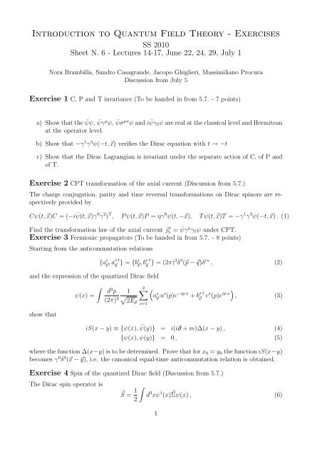
Introduction to Quantum Field Theory - Exercises
SS 2010
Sheet N. 6 - Lectures 14-17, June 22, 24, 29, July 1
Nora Brambilla, Sandro Casagrande, Jacopo Ghiglieri, Massimiliano Procura
Discussion from July 5
Exercise 1 C, P and T invariance (To be handed in from 5.7. - 7 points)
a) Show that the ¯ ψψ, ¯ ψγ µ ψ, ¯ ψσ µν ψ and i ¯ ψγ5ψ are real at the classical level and Hermitean
at the operator level.
b) Show that −γ 1 γ 3 ψ(−t, x) verifies the Dirac equation with t → −t
c) Show that the Dirac Lagrangian is invariant under the separate action of C, of P and
of T.
Exercise 2 CPT transformation of the axial current (Discussion from 5.7.)
The charge conjugation, parity and time reversal transformations on Dirac spinors are respectively
provided by
Cψ(t, x)C = (−i ¯ ψ(t, x)γ 0 γ 2 ) T , P ψ(t, x)P = ηγ 0 ψ(t, −x), T ψ(t, x)T = −γ 1 γ 3 ψ(−t, x) . (1)
Find the transformation law of the axial current j µ
5 = ¯ ψγ µ γ5ψ under CPT.
Exercise 3 Fermionic propagators (To be handed in from 5.7. - 8 points)
Starting from the anticommutation relations
and the expression of the quantized Dirac field
show that
ψ(x) =
{a r s †
p, aq } = {br s †
p, bq } = (2π)3δ 3 (p − q)δ rs , (2)
d 3 p
(2π) 3
1
2Ep
2
s=1
a s p u s (p)e −ip·x s †
+ bp vs (p)e ip·x
, (3)
iS(x − y) ≡ {ψ(x), ¯ ψ(y)} = i(i/∂ + m)∆(x − y) , (4)
{ψ(x), ψ(y)} = 0 , (5)
where the function ∆(x−y) is to be determined. Prove that for x0 = y0 the function iS(x−y)
becomes γ 0 δ 3 (x − y), i.e. the canonical equal-time anticommutation relation is obtained.
Exercise 4 Spin of the quantized Dirac field (Discussion from 5.7.)
The Dirac spin operator is
S = 1
2
d 3 xψ † (x) Σψ(x) , (6)
1

where Σi = 1
2ɛijkS jk . By substituting the expression (3) in (6), prove that in the rest frame
s †
(p = 0) the state created by ap with s = 1 has Sz = +1/2, while the one with s = 2 has
Sz = −1/2. Prove also that for the antiparticles the opposite happens: the state created by
s †
bp with s = 1 has Sz = −1/2 and viceversa.
Exercise 5 Four-point function (Discussion from 5.7.)
Calculate 〈0| ¯ ψ(x1)ψ(x2)ψ(x3) ¯ ψ(x4)|0〉 for free fields. The result should be expressed in terms
of vacuum expectation values of two fields.
Exercise 6 On the electromagnetic field (To be handed in from 5.7. - 15 points)
• Calculate the commutator
in the Lorentz gauge.
iD µν (x − y) = [A µ (x), A ν (y)] , (7)
• Calculate the following commutators between components of the electric and magnetic
fields:
[E i (x), E j (y)] , [B i (x), B j (y)] , [E i (x), B j (y)] . (8)
(Hint: use the Lorentz gauge when you express E i and B i in terms of the field A µ .)
Calculate these commutators also for equal times, x 0 = y 0 .
• Calculate
〈0|{E i (x), B j (y)}|0〉 , 〈0|{B i (x), B j (y)}|0〉 , 〈0|{E i (x), E j (y)}|0〉 . (9)
(Hint: start with the Fourier decompositions of E and B in terms of creation and
annihilation operators.)
Exercise 7 Projectors (Discussion from 5.7.)
Consider
where ¯ k µ = (k 0 , − k). Calculate:
if k 2 = 0.
P µν = g µν − kµ¯ k ν + k ν¯ k µ
k · ¯ k
, P µν
⊥ = kµ¯ k ν + k ν¯ k µ
k · ¯ k
P µν Pνσ , P µν
⊥ P ⊥ νσ , P µν + P µν
⊥ , gµνPµν , g µν P ⊥ µν , P µ ν P νσ
⊥
Exercise 8 Massive vector fields (Reading exercise - Discussion from 5.7.)
Consider the Proca Lagrangian
(10)
(11)
L = − 1
4 FµνF µν + 1
2 m2 AµA µ . (12)
2

Verify that it is not gauge invariant and show that the equations of motion are
(∂ 2 + m 2 )A µ = 0 and ∂µA µ = 0 . (13)
Perform a canonical quantization and verify that the theory describes a spin 1 particle.
Exercise 9 Thermal QFT (Reading exercise - Discussion from 5.7.)
Let H be a second quantized Hamiltonian of a free, real scalar field and β a real parameter.
a) Prove the identity
e −βH a † (p) = a † (p)e −β(H+Ep) . (14)
Hint: To this end either apply both sides to a state |p1, pn〉, or define a function
f(β) given by the difference of the two sides. You have f(0) = 0, calculate [H, a(p) † ] =
Epa(p) † and obtain that the derivative of f(β) is −Hf(β). The solution of this equation
with the boundary condition f(0) = 0 is f(β) = 0. This is a very general method to
show operator equalities.
b) According to quantum mechanics the expectation value of any operator O in a mixed
state described by a density matrix ρ is given by Tr(ρO) where ρ is normalized to
Tr(ρ) = 1. In a thermal state with temperature T = 1/β the density matrix is given
by ρ = e −βH / Tr(e −βH ) and therefore the thermal expectation values are defined as
〈O〉β = Tr(Oe−βH )
Tr(e −βH )
, (15)
where the trace is taken over all Fock states. Using the result from part a) show that
Then in a finite volume V we have
〈a † (q) a(q)〉β = (2π)3 δ 3 (p − q)
e βEp − 1
〈a † (p) a(p)〉β =
. (16)
V
eβEp . (17)
− 1
This shows that a(p) † / √ V creates quanta obeying the Bose-Einstein distribution.
c) Repeat the exercise for anticommuting operators and verify that one obtains Fermi
statistics.
Exercise 10 Bogoliubov transformation (Reading exercise - Discussion from 5.7.)
Consider a gas of N electrons in a box of volume V .
a) Show that in the ground state the electrons fill all states with momenta |p| < pF ,
given by N/V = p 3 F /(3π2 ). The state with all levels filled up to pF is called the Fermi
vacuum and we denote it with |0〉F to distinguish it from the Fock vacuum |0〉 where
simply all states are empty. The Fermi vacuum is the vacuum state of the system with
subject to the constraint of a fixed number of particles N, while the Fock vacuum is
the vacuum state of the system with no constraint on the particle number.
3

) Let a(p, s), a † (p, s) be the usual annihilation and creation operators of the the electron,
so by definition a(p, s)|0〉 = 0 ∀p, s. Verify that it is not true that a(p, s)|0〉F = 0 ∀p, s.
That means a † (p, s) is not the appropriate operator to describe excitations above |0〉F .
c) Define
A(p, s) = θ(|p| − pF )a(p, s) + θ(pF − |p|)a † (−p, −s) , (18)
and A † (p, s) correspondingly. Verify that A(p, s)|0〉F = 0 ∀p, s, and that A(p, s) and
A † (q, r) still satisfy canonical anticommutation relations. Give a physical interpretation
of the action of A † (q, r) on |0〉F .
Equation (18) is a particular case of a Bogoliubov transformation which can be defined for
both bosonic and fermionic operators as
A(p, s) = αp a(p, s) − βp a † (−p, −s) , (19)
and A † (p, s) correspondingly with αp and βp complex coefficients.
d) Show that the condition that A(p, s) and A † (p, s) satisfy the canonical commutation
relations, requires that
|αp| 2 ∓ |βp| 2 = 1 and αpβ−p ∓ α−pβp = 0 . (20)
The minus sign applies to the case of bosons, whereas the plus applies for fermions.
e) Consider the spin zero case. We have two different types of particles: a-particles
obtained by applying a † (p) on |0〉a and the A-particles obtained by acting with A † (p)
on |0〉A (the vacua are generalizations of |0〉 and |0〉F ). Setting V = 1 the respective
particle number operators are a † (p)a(p) and A † (p)A(p). Let |np〉 be an eigenstate of
the operator a † (p)a(p) with eigenvalue np. Show that
Np ≡ 〈np|A † (p)A(p)|np〉 = np + 2|βp| 2
np + 1
. (21)
2
Thus in particular the vacuum of the a-particles has Np = |βp| 2 . This means that
in terms of A-particles the vacuum of the a-particles is a multiparticle state. States
created by A † are often called quasiparticle states.
Bogoliubov transformations of this type are used in condensed matter physics, in the context
of superfluidity or superconductivity, in cosmology, and in QCD.
4