- Page 1 and 2: CONTROi I naiysis ana uesign (4)WIL
- Page 3 and 4: Copyright © 2003 by John Wiley & S
- Page 6 and 7: Contents 1 Introduction 1 1.1 Linea
- Page 8 and 9: CONTENTS ix 3.8 The Invariance Prin
- Page 10 and 11: CONTENTS xi 8.1 Power and Energy: P
- Page 12: CONTENTS xiii A Proofs 307 A.1 Chap
- Page 15 and 16: xvi 8, along with some of the most
- Page 18 and 19: Chapter 1 Introduction This first c
- Page 20 and 21: 1.2. NONLINEAR SYSTEMS 3 with A=[-o
- Page 22 and 23: 1.3. EQUILIBRIUM POINTS 5 1.3 Equil
- Page 24 and 25: 1.4. FIRST-ORDER AUTONOMOUS NONLINE
- Page 26 and 27: 1.5. SECOND-ORDER SYSTEMS: PHASE-PL
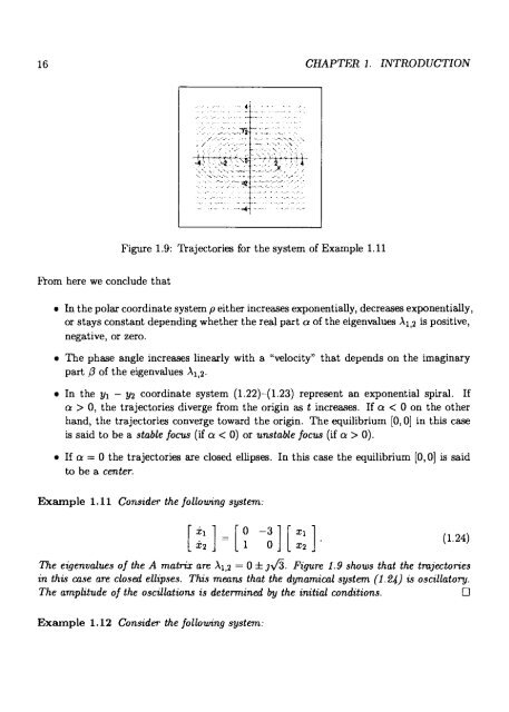
- Page 28 and 29: 1.6. PHASE-PLANE ANALYSIS OF LINEAR
- Page 30 and 31: 1.6. PHASE-PLANE ANALYSIS OF LINEAR
- Page 34 and 35: 1.6. PHASE-PLANE ANALYSIS OF LINEAR
- Page 36 and 37: 1.7. PHASE-PLANE ANALYSIS OF NONLIN
- Page 38 and 39: 1.8. HIGHER-ORDER SYSTEMS 1.8.1 Cha
- Page 40 and 41: 1.9. EXAMPLES OF NONLINEAR SYSTEMS
- Page 42 and 43: 1.9. EXAMPLES OF NONLINEAR SYSTEMS
- Page 44 and 45: 1.10. EXERCISES 27 Figure 1.18: Bal
- Page 46 and 47: 1.10. EXERCISES 29 m2 Figure 1.19:
- Page 48 and 49: Chapter 2 Mathematical Preliminarie
- Page 50 and 51: 2.3. VECTOR SPACES 33 (3) 3 0 E X :
- Page 52 and 53: 2.3. VECTOR SPACES 35 where the 1 e
- Page 54 and 55: 2.3. VECTOR SPACES 37 Proof: First
- Page 56 and 57: 2.4. MATRICES 39 2.4 Matrices We as
- Page 58 and 59: 2.4. MATRICES 41 Proof: By definiti
- Page 60 and 61: 2.4. MATRICES 43 (i) A is positive
- Page 62 and 63: 2.6. SEQUENCES 45 Compact set: A se
- Page 64 and 65: 2.7. FUNCTIONS 47 If f is a functio
- Page 66 and 67: 2.8. DIFFERENTIABILITY 2.8 Differen
- Page 68 and 69: 2.8. DIFFERENTIABILITY 51 Theorem 2
- Page 70 and 71: 2.9. LIPSCHITZ CONTINUITY 53 Notice
- Page 72 and 73: 2.10. CONTRACTION MAPPING 55 and th
- Page 74 and 75: 2.11. SOLUTION OF DIFFERENTIAL EQUA
- Page 76 and 77: 2.12. EXERCISES 59 Denoting t1 = to
- Page 78 and 79: 2.12. EXERCISES 61 (2.10) Show that
- Page 80: 2.12. EXERCISES 63 Notes and Refere
- Page 83 and 84:
66 CHAPTER 3. LYAPUNOV STABILITY I.
- Page 85 and 86:
68 CHAPTER 3. LYAPUNOV STABILITY I.
- Page 87 and 88:
70 CHAPTER 3. LYAPUNOV STABILITY I.
- Page 89 and 90:
72 CHAPTER 3. LYAPUNOV STABILITY I:
- Page 91 and 92:
74 CHAPTER 3. LYAPUNOV STABILITY I.
- Page 93 and 94:
76 CHAPTER 3. LYAPUNOV STABILITY I:
- Page 95 and 96:
78 CHAPTER 3. LYAPUNOV STABILITY I:
- Page 97 and 98:
80 CHAPTER 3. LYAPUNOV STABILITY I.
- Page 99 and 100:
82 CHAPTER 3. LYAPUNOV STABILITY I.
- Page 101 and 102:
84 CHAPTER 3. LYAPUNOV STABILITY I.
- Page 103 and 104:
86 CHAPTER 3. LYAPUNOV STABILITY I.
- Page 105 and 106:
88 CHAPTER 3. LYAPUNOV STABILITY I:
- Page 107 and 108:
90 CHAPTER 3. LYAPUNOV STABILITY I.
- Page 109 and 110:
92 CHAPTER 3. LYAPUNOV STABILITY I:
- Page 111 and 112:
94 CHAPTER 3. LYAPUNOV STABILITY I.
- Page 113 and 114:
96 CHAPTER 3. LYAPUNOV STABILITY I:
- Page 115 and 116:
98 CHAPTER 3. LYAPUNOV STABILITY I.
- Page 117 and 118:
100 CHAPTER 3. LYAPUNOV STABILITY I
- Page 119 and 120:
102 CHAPTER 3. LYAPUNOV STABILITY I
- Page 121 and 122:
104 CHAPTER 3. LYAPUNOV STABILITY I
- Page 123 and 124:
106 CHAPTER 3. LYAPUNOV STABILITY I
- Page 125 and 126:
108 CHAPTER 4. LYAPUNOV STABILITY H
- Page 127 and 128:
110 CHAPTER 4. LYAPUNOV STABILITY I
- Page 129 and 130:
112 CHAPTER 4. LYAPUNOV STABILITY I
- Page 131 and 132:
114 CHAPTER 4. LYAPUNOV STABILITY I
- Page 133 and 134:
116 CHAPTER 4. LYAPUNOV STABILITY I
- Page 135 and 136:
118 CHAPTER 4. LYAPUNOV STABILITY I
- Page 137 and 138:
120 CHAPTER 4. LYAPUNOV STABILITY I
- Page 139 and 140:
122 CHAPTER 4. LYAPUNOV STABILITY I
- Page 141 and 142:
124 CHAPTER 4. LYAPUNOV STABILITY I
- Page 143 and 144:
126 CHAPTER 4. LYAPUNOV STABILITY H
- Page 145 and 146:
128 CHAPTER 4. LYAPUNOV STABILITY I
- Page 147 and 148:
130 CHAPTER 4. LYAPUNOV STABILITY I
- Page 149 and 150:
132 CHAPTER 4. LYAPUNOV STABILITY I
- Page 151 and 152:
134 CHAPTER 4. LYAPUNOV STABILITY I
- Page 154 and 155:
Chapter 5 Feedback Systems So far,
- Page 156 and 157:
5.1. BASIC FEEDBACK STABILIZATION 1
- Page 158 and 159:
5.2. INTEGRATOR BACKSTEPPING 141 5.
- Page 160 and 161:
5.2. INTEGRATOR BACKSTEPPING 143 De
- Page 162 and 163:
5.3. BACKSTEPPING: MORE GENERAL CAS
- Page 164 and 165:
5.3. BACKSTEPPING: MORE GENERAL CAS
- Page 166 and 167:
5.3. BACKSTEPPING: MORE GENERAL CAS
- Page 168 and 169:
5.4. EXAMPLE 151 5.4 Example 8 Figu
- Page 170 and 171:
5.5. EXERCISES 153 [S - 0(x)] = x1
- Page 172 and 173:
Chapter 6 Input-Output Stability So
- Page 174 and 175:
6.1. FUNCTION SPACES 157 Both L2 an
- Page 176 and 177:
6.2. INPUT-OUTPUT STABILITY 159 Thu
- Page 178 and 179:
6.2. INPUT-OUTPUT STABILITY 161 (a)
- Page 180 and 181:
6.2. INPUT-OUTPUT STABILITY 163 1.2
- Page 182 and 183:
6.3. LINEAR TIME-INVARIANT SYSTEMS
- Page 184 and 185:
6.4. L GAINS FOR LTI SYSTEMS where
- Page 186 and 187:
6.5. CLOSED-LOOP INPUT-OUTPUT STABI
- Page 188 and 189:
6.6. THE SMALL GAIN THEOREM 171 In
- Page 190 and 191:
6.6. THE SMALL GAIN THEOREM 173 N(x
- Page 192 and 193:
6.7. LOOP TRANSFORMATIONS 175 Figur
- Page 194 and 195:
6.7. LOOP TRANSFORMATIONS 177 U l M
- Page 196 and 197:
6.8. THE CIRCLE CRITERION 179 (i) g
- Page 198 and 199:
6.9. EXERCISES 181 (6.3) Prove the
- Page 200 and 201:
Chapter 7 Input-to-State Stability
- Page 202 and 203:
7.2. DEFINITIONS 185 Setting u = 0,
- Page 204 and 205:
7.3. INPUT-TO-STATE STABILITY (ISS)
- Page 206 and 207:
7.3. INPUT-TO-STATE STABILITY (ISS)
- Page 208 and 209:
7.4. INPUT-TO-STATE STABILITY REVIS
- Page 210 and 211:
7.4. INPUT-TO-STATE STABILITY REVIS
- Page 212 and 213:
7.5. CASCADE-CONNECTED SYSTEMS U E2
- Page 214 and 215:
7.5. CASCADE-CONNECTED SYSTEMS 197
- Page 216:
7.6. EXERCISES 199 (i) Is it locall
- Page 219 and 220:
202 CHAPTER 8. PASSIVITY v i Figure
- Page 221 and 222:
204 CHAPTER 8. PASSIVITY Moreover,
- Page 223 and 224:
206 CHAPTER 8. PASSIVITY Definition
- Page 225 and 226:
208 CHAPTER 8. PASSIVITY Thus (UT,
- Page 227 and 228:
210 CHAPTER 8. PASSIVITY Thus, H f
- Page 229 and 230:
212 CHAPTER 8. PASSIVITY Under thes
- Page 231 and 232:
214 CHAPTER 8. PASSIVITY Under thes
- Page 233 and 234:
216 CHAPTER 8. PASSIVITY (i) H is p
- Page 235 and 236:
218 CHAPTER 8. PASSIVITY Definition
- Page 237 and 238:
220 CHAPTER 8. PASSIVITY Example 8.
- Page 240 and 241:
Chapter 9 Dissipativity In Chapter
- Page 242 and 243:
9.2. DIFFERENTIABLE STORAGE FUNCTIO
- Page 244 and 245:
9.3. QSR DISSIPATIVITY 227 Definiti
- Page 246 and 247:
9.4. EXAMPLES 229 5- Very strictly-
- Page 248 and 249:
9.5. AVAILABLE STORAGE 9.4.2 Mass-S
- Page 250 and 251:
9.6. ALGEBRAIC CONDITION FOR DISSIP
- Page 252 and 253:
9.6. ALGEBRAIC CONDITION FOR DISSIP
- Page 254 and 255:
9.7. STABILITY OF DISSIPATIVE SYSTE
- Page 256 and 257:
9.8. FEEDBACK INTERCONNECTIONS 239
- Page 258 and 259:
9.8. FEEDBACK INTERCONNECTIONS 241
- Page 260 and 261:
9.9. NONLINEAR G2 GAIN 9.9 Nonlinea
- Page 262 and 263:
9.9. NONLINEAR L2 GAIN 245 (iii) IH
- Page 264 and 265:
9.10. SOME REMARKS ABOUT CONTROL DE
- Page 266 and 267:
9.10. SOME REMARKS ABOUT CONTROL DE
- Page 268 and 269:
9.11. NONLINEAR L2-GAIN CONTROL 251
- Page 270 and 271:
9.12. EXERCISES 253 9.12 Exercises
- Page 272 and 273:
Chapter 10 Feedback Linearization I
- Page 274 and 275:
10.1. MATHEMATICAL TOOLS 257 Lfh(x)
- Page 276 and 277:
10.1. MATHEMATICAL TOOLS 259 10.1.3
- Page 278 and 279:
10.1. MATHEMATICAL TOOLS 261 and su
- Page 280 and 281:
10.1. MATHEMATICAL TOOLS 263 Defini
- Page 282 and 283:
10.2. INPUT-STATE LINEARIZATION 265
- Page 284 and 285:
10.2. INPUT-STATE LINEARIZATION 267
- Page 286 and 287:
10.2. INPUT-STATE LINEARIZATION and
- Page 288 and 289:
10.3. EXAMPLES 271 provided that wh
- Page 290 and 291:
10.4. CONDITIONS FOR INPUT-STATE LI
- Page 292 and 293:
10.5. INPUT-OUTPUT LINEARIZATION 27
- Page 294 and 295:
10.5. INPUT-OUTPUT LINEARIZATION 27
- Page 296 and 297:
10.5. INPUT-OUTPUT LINEARIZATION 27
- Page 298 and 299:
10.6. THE ZERO DYNAMICS 281 i=Ax+Bu
- Page 300 and 301:
10.6. THE ZERO DYNAMICS 283 that th
- Page 302 and 303:
10.6. THE ZERO DYNAMICS 285 Definit
- Page 304 and 305:
10.7. CONDITIONS FOR INPUT-OUTPUT L
- Page 306:
10.8. EXERCISES 289 (10.8) Consider
- Page 309 and 310:
292 CHAPTER 11. NONLINEAR OBSERVERS
- Page 311 and 312:
294 CHAPTER 11. NONLINEAR OBSERVERS
- Page 313 and 314:
296 CHAPTER 11. NONLINEAR OBSERVERS
- Page 315 and 316:
298 CHAPTER 11. NONLINEAR OBSERVERS
- Page 317 and 318:
300 CHAPTER 11. NONLINEAR OBSERVERS
- Page 319 and 320:
302 CHAPTER 11. NONLINEAR OBSERVERS
- Page 321 and 322:
304 CHAPTER 11. NONLINEAR OBSERVERS
- Page 323 and 324:
306 CHAPTER 11. NONLINEAR OBSERVERS
- Page 325 and 326:
308 APPENDIX A. PROOFS (ii) It is c
- Page 327 and 328:
310 APPENDIX A. PROOFS For the conv
- Page 329 and 330:
312 APPENDIX A. PROOFS 9V ax-1 xz 9
- Page 331 and 332:
314 APPENDIX A. PROOFS Since the eq
- Page 333 and 334:
316 APPENDIX A. PROOFS Proof: The n
- Page 335 and 336:
318 APPENDIX A. PROOFS We have x Fi
- Page 337 and 338:
320 APPENDIX A. PROOFS (b) 0 = a ,3
- Page 339 and 340:
322 APPENDIX A. PROOFS To this end
- Page 341 and 342:
324 A.5 Chapter 8 APPENDIX A. PROOF
- Page 343 and 344:
326 APPENDIX A. PROOFS and substitu
- Page 345 and 346:
328 APPENDIX A. PROOFS It follows t
- Page 347 and 348:
330 APPENDIX A. PROOFS A.7 Chapter
- Page 349 and 350:
332 APPENDIX A. PROOFS Assume now t
- Page 351 and 352:
334 APPENDIX A. PROOFS Multiplying
- Page 354 and 355:
Bibliography [1] B. D. O. Anderson
- Page 356 and 357:
BIBLIOGRAPHY 339 [27] W. Hahn, Stab
- Page 358 and 359:
BIBLIOGRAPHY 341 [58] E. Ott, Chaos
- Page 360:
BIBLIOGRAPHY 343 [87] A. van der Sc
- Page 363 and 364:
346 LIST OF FIGURES 3.1 Stable equi
- Page 366 and 367:
Index Absolute stability, 179 Asymp
- Page 368 and 369:
INDEX discrete-time, 132 nonautonom