Métodos miméticos de pasos fraccionarios - E-Archivo - Universidad ...

§2.3 spatial semidiscretization: a cell-node mfd method 13
recently proposed in Shashkov and Steinberg (1995, 1996) and Hyman et al.
(1997, 2002).
More precisely, the semidiscretization process may be outlined as follows.
First, we introduce the vector spaces of semidiscrete scalar and vector functions
approximating Hs and Hv, respectively. Then, a discrete analogue of the divergence
operator D is deduced from the coordinate invariant definition of the
divergence, based on Gauss’s divergence theorem:
div w = lim
|V |→0
1
|V |
∂V
⟨w, n⟩ ds, (2.12)
where |V | denotes the area of a given region V with boundary ∂V . We next
define discrete approximations to the scalar and vector inner products given in
(2.4) and (2.9), respectively. The discrete analogue of the gradient operator G
is then obtained by requiring it to be the adjoint of the discrete divergence, thus
imposing a discrete version of (2.10). Finally, we properly approximate K in
order to define a discrete analogue of the product KG. The approximation to
the elliptic operator A = DKG trivially follows from the previous discretizations,
giving rise to an MFD semidiscrete scheme for (2.1). This mimetic technique
is based on the so-called support-operator method, which considers the discrete
divergence as a primary operator that supports the construction of the discrete
gradient, usually referred to as the derived operator (cf. Shashkov (1996) and
references therein).
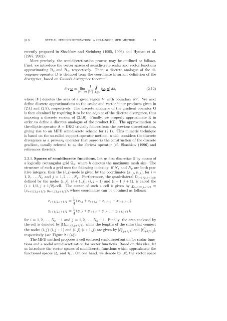
2.3.1. Spaces of semidiscrete functions. Let us first discretize Ω by means of
a logically rectangular grid Ωh, where h denotes the maximum mesh size. The
structure of such a grid uses the following indexing: if Nx and Ny are both positive
integers, then the (i, j)-node is given by the coordinates (xi,j, yi,j), for i =
1, 2, . . . , Nx and j = 1, 2, . . . , Ny. Furthermore, the quadrilateral Ω i+1/2,j+1/2,
defined by the nodes (i, j), (i + 1, j), (i, j + 1) and (i + 1, j + 1), is called the
(i + 1/2, j + 1/2)-cell. The center of such a cell is given by x i+1/2,j+1/2 ≡
(x i+1/2,j+1/2, y i+1/2,j+1/2), whose coordinates can be obtained as follows:
x i+1/2,j+1/2 = 1
4 (xi,j + xi+1,j + xi,j+1 + xi+1,j+1),
y i+1/2,j+1/2 = 1
4 (yi,j + yi+1,j + yi,j+1 + yi+1,j+1),
for i = 1, 2, . . . , Nx − 1 and j = 1, 2, . . . , Ny − 1. Finally, the area enclosed by
the cell is denoted by |Ωi+1/2,j+1/2|, while the lengths of the sides that connect
the nodes (i, j)-(i, j + 1) and (i, j)-(i + 1, j) are given by |ℓα i,j+1/2 | and |ℓβ i+1/2,j |,
respectively (see Figure 2.1 (a)).
The MFD method proposes a cell-centered semidiscretization for scalar functions
and a nodal semidiscretization for vector functions. Based on this idea, let
us introduce the vector spaces of semidiscrete functions which approximate the
functional spaces Hs and Hv. On one hand, we denote by Hs the vector space