Métodos miméticos de pasos fraccionarios - E-Archivo - Universidad ...

§2.5 numerical experiments 29
y
1
0.8
0.6
0.4
0.2
0
0 0.2 0.4
x
0.6 0.8 1
y
1
0.8
0.6
0.4
0.2
0
0 0.2 0.4
x
0.6 0.8 1
y
1
0.8
0.6
0.4
0.2
0
0 0.2 0.4
x
0.6 0.8 1
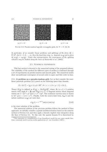
(a) N = 17 (b) N = 33 (c) N = 65
Figure 2.8: Pseudo-random logically rectangular grids, for N = 17, 33, 65.
In particular, if we consider linear problems and splittings of the form A h k =
Γ h k Ah , for k = 1, 2, . . . , m, then the local time step, τk, depends on x and is given
by τk(x) = τρk(x). Under this interpretation, the convergence of the splitting
schemes may be studied along the lines of Samarskiĭ et al. (2002).
2.5. Numerical experiments
This last section is devoted to the numerical testing of the proposed scheme.
The reliability of the method for different types of meshes is confirmed through
a set of experiments on pseudo-random and smooth grids. The numerical results
show unconditional convergence of second order in space and first order in time.
2.5.1. A problem on a pseudo-random grid. Let us first consider the semilinear
parabolic problem (2.1) posed on the following space-time domain:
Ω × (0, T ] = {x ≡ (x, y) ∈ R 2 : 0 < x < 1, 0 < y < 1} × (0, 1].
Tensor K(x) is defined as K(x) = RθD(x)RT θ , where Rθ is a 2 × 2 rotation
matrix with angle θ = 5π and D(x) is a 2 × 2 diagonal matrix whose diagonal
12
entries are 1 + 2x2 + y2 and 1 + x2 + 2y2 . The nonlinear reaction term is chosen
to be5 g(ψ) = 1/(1 + ψ3 ). Finally, both the source/sink term f(x, t) and the
initial condition ψ0(x) are such that:
ψ(x, t) = e −2π2 t sin(πx) sin(πy) (2.45)
is the exact solution of the problem.
The numerical solution of the previous problem follows the method of lines
approach: we initially consider a spatial semidiscretization based on the mimetic
method of Section 2.3, and then apply a linearly implicit time integrator along
the lines of Section 2.4. To this end, the spatial domain Ω is discretized by
5 This expression is a simplification of van Genuchten’s model for root water uptake functions,
commonly used in porous media applications (cf. van Genuchten (1987)).