Métodos miméticos de pasos fraccionarios - E-Archivo - Universidad ...

§2.4 time integration: a linearly implicit fsrkm+1 method 23
S 1,−1
i+1/2,j+1/2
S 1,0
i+1/2,j+1/2
S 1,1
i+1/2,j+1/2
KXX
= −
4(hX )
Y
i+1,j KXY i+1,j KY i+1,j
+ − 2 Y
2h X h
4(hY ,
) 2
i+1,j + KXX i+1,j+1
= −KXX
4(hX ) 2 + KY Y
Y
i+1,j + KY i+1,j+1
4(hY ) 2
= −KXX
4(hX )
Y
i+1,j+1 KXY i+1,j+1 KY i+1,j+1
− − 2 Y
2h X h
4(hY .
) 2
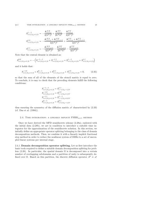
Note that the central element is obtained as:
S 0,0
(
i+1/2,j+1/2 = − S −1,−1
)
i+1/2,j+1/2 + S−1,1
i+1/2,j+1/2 + S1,−1
i+1/2,j+1/2 + S1,1
i+1/2,j+1/2
and it holds that:
S −1,0
i+1/2,j+1/2 + S0,−1
i+1/2,j+1/2 + S0,1
i+1/2,j+1/2 + S1,0
i+1/2,j+1/2 = 0, (2.35)
so that the sum of all of the elements of the stencil matrix is equal to zero.
To conclude, it is easy to check that the preceding elements fulfill the following
conditions:
S −1,−1
i+1/2,j+1/2 = S1,1
i−1/2,j−1/2 ,
S −1,0
i+1/2,j+1/2 = S1,0
i−1/2,j+1/2 ,
S −1,1
i+1/2,j+1/2 = S1,−1
i−1/2,j+3/2 ,
S 0,−1
i+1/2,j+1/2 = S0,1
i+1/2,j−1/2 ,
thus ensuring the symmetry of the diffusion matrix A characterized by (2.33)
(cf. Das et al. (1994)).
2.4. Time integration: a linearly implicit FSRKm+1 method
Once we have derived the MFD semidiscrete scheme (2.28a), endowed with
the initial data (2.28b), we are in condition to introduce a suitable time integrator
for the approximation of the semidiscrete solution. In this section, we
initially define an appropriate operator splitting belonging to the class of domain
decomposition methods. Then, we combine it with a linearly implicit fractional
step method in order to reduce the nonlinear system of ODEs to a set of uncoupled
linear systems per internal stage.
2.4.1. Domain decomposition operator splitting. Let us first introduce the
basic tools required to define a suitable domain decomposition splitting for problem
(2.28). In particular, the spatial domain Ω is decomposed into a certain
number of overlapping subdomains and a partition of unity is subsequently defined
over Ω. Based on this partition, the discrete diffusion operator A h ≡ A
,