tesi R. Valiante.pdf - EleA@UniSA

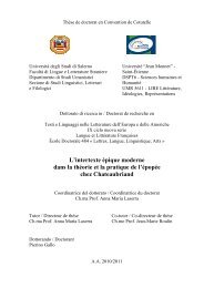
Unione Europea Università degli Studi di Salerno
DIPARTIMENTO DI INGEGNERIA MECCANICA
Dottorato di Ricerca in Ingegneria Meccanica
IX Ciclo N.S. (2007-2010)
“Innovative techniques for Structural Health Monitoring: a
theoretical and experimental study”
Ing. Rossella Valiante
Tutor: Coordinatore:
Prof. Domenico Guida
Prof. Vincenzo Sergi
Co-Tutor:
Prof. Fernando Fraternali
Ing. Generoso Iannuzzo (Alenia)

The The present present work, work, carried carried out out at at Alenia Alenia Aeronautica,
Aeronautica,
contains contains sensitive sensitive information information and and data data covered covered bby
b y the
Intellect Intellectually Intellect ually Property Property Rights. Rights. Therefore, Therefore, the the use use use of
of
such such information information and and data data is is allowed allowed only only under under
under
permission permission permission of of of Alenia Alenia Alenia Aeronautica.
Aeronautica.
Aeronautica.

RINGRAZIAMENTI
E’ per me doveroso, oltre che sentito, ringraziare l’ing. Iannuzzo, il quale,
oltre ad avermi supportato come tutor nella stesura del presente lavoro, mi ha,
innanzitutto, concesso la preziosa possibilità di affrontare quest’avventura.
Vorrei, inoltre, dire il mio forte grazie al prof. Guida che, non pago di
avermi sopportato durante la tesi di laurea, mi ha invogliato a tentare questo
arduo percorso, ancora una volta sotto la sua guida.
Un ringraziamento particolare lo dedico al prof. Fraternali, il quale mi ha
fornito lo sprone necessario a seguitare col lavoro di dottorato, oltre ad avermi
guidata attentamente nella stesura dello stesso.
Non posso dimenticare il prof. Ruzzene, che mi ha introdotto nel mondo
delle onde di Lamb, né la sua collaboratrice, Nicole Apetre, la quale tanti
preziosi consigli sulla modellazione numerica delle stesse mi ha dispensato.
Tengo particolarmente a ringraziare il Prof. D’Agostino che, col garbo che
lo contraddistingue, ha seguito, seppur da lontano, quest’altro mio percorso di
studi, dandomi sempre l’impagabile sensazione di sentirmi a casa ogniqualvolta
mettessi piede a Fisciano.
Ringrazio il nostro Coordinatore, Prof. Vincenzo Sergi, per la gestione
ineccepibile del corso di dottorato, accompagnata sempre da atteggiamento
disponibile e cortese.

Dico grazie infinite a Pierpaolo D’Agostino, che mi ha più volte salvato dal
panico ‘da dottorato’, oltre che aiutato fattivamente in questi tre anni sempre col
sorriso sulle labbra. Grazie, Pierpaolo!
Non posso dimenticare Luca, Rosario, e tutte le persone coinvolte nel
coordinamento del corso, né i miei colleghi d’avventura, Roberta, Marzia, Gino,
Renzo, sempre disponibili e gentili.
Vorrei, inoltre, ringraziare il collega Michele Rotondano, per il suo
fondamentale contributo informatico.
Un mega grazie va alla mia amica, nonché collega, Maria Pagano, per la
preziosa collaborazione ed il supporto morale! Merci, Mary!
Particolarmente doveroso ed al contempo piacevole per me ringraziare
Damiano Laurenza, il quale mi ha fornito aiuto concreto, oltre ad avermi
spronata ad ogni ostacolo incontrato sulla via. Grazie!
Tengo a dire grazie alle mie super amiche Ylenia e Stefania, per
l’incoraggiamento continuo ricevuto, sempre e comunque. Grazie, tesorucce!
Ringrazio l’Amico cui devo moltissimo, don Dolindo; un ringraziamento
particolare lo dedico a don Peppino, imprescindibile presenza di questi anni.
Un grazie speciale lo dedico alla persona più che speciale che mi ha
letteralmente sopportato, oltreché sopportato in questo periodo, con una presenza
delicata e costante. Grazie di cuore.

Vorrei, infine, disporre del vocabolario di Dante per dire grazie alle persone
della mia famiglia, papà, mamma e Pina, le quali mi hanno dato, ciascuna a
proprio distintivo ed unico modo, la forza di raggiungere il traguardo. Vi amo.

A PAPÀ, MAMMA E PINA,
RISPETTIVAMENTE IL MIO CUORE,
LA MIA ANIMA E
LA MIA GEMELLA SIAMESE

CONTENTS
Abstract of dissertation .......................................................................... 7
1. Introduction...................................................................................10
1.1. General SHM Paradigm ....................................................................12
1.2. Definition of Damage in CFRP Composite Components......................13
1.3. Global versus Local SHM Approaches................................................15
1.4. Vibration-Based Vs Guided Waves-Based Techniques: Our Choice .....16
1.5. Vibration-Based Damage Measures ..................................................18
1.5.1. Frequency changes................................................................. 18
1.5.2. Mode shape changes .............................................................. 20
1.5.3. Mode shape curvature changes .............................................. 21
1.6. Guided Waves-Based Damage Measures...........................................23
1.7. Theory of waves in elastic media ......................................................24
1.7.1. Waves in taut string ............................................................... 24
1.7.2. String on an elastic base – Dispersion ................................... 28
1.7.1. Group Velocity....................................................................... 34
1.7.1. Wave in plates - Lamb waves ................................................ 37
2. Innovative SHM Techniques based on SLDV measures ....................43
2.1. Damage measure based on Energy functional distribution ................44
2.2. Interpolation of the measured response and synthesis of the
undamaged baseline ...................................................................................46
2.3. Strain Energy Distributuion...............................................................48
2.4. Filtering of signals in domain wavenumber / frequency.....................49
3. Experimental Analysis ....................................................................53
3.1. Description of the measure set up ....................................................56
3.2. Acquisition parameters ....................................................................56
3.3. Results.............................................................................................60
3.3.1. Skin External Side.................................................................. 62
3.3.2. Skin Internal Side ‘1’............................................................. 63
3.3.3. Web Side ‘1’ .......................................................................... 66
3.3.4. Skin Internal Side ‘2’............................................................. 68
3.3.5. Web Side ‘2’ .......................................................................... 70
3.4. Analysis of the wavelenghts generated.............................................72

2
3.5. First Conclusions ..............................................................................74
3.6. Elaboration of the SLDV data previoulsy observed ............................76
3.6.1. Skin External Side.................................................................. 76
3.6.2. Skin Internal Side ‘1’............................................................. 79
3.6.3. Skin Internal Side ‘2’............................................................. 82
3.6.4. Web Sides ‘1’ e ‘2’ ............................................................... 85
3.7. Comparative Analysis of the Signals recorded on the opposite sides of
the web ......................................................................................................91
3.8. Analysis of further Polytec data ........................................................96
3.8.1. Test and Item description....................................................... 97
3.9. Results recorded by Polytec with a 3D vibrometer over a plate with
defects........................................................................................................99
3.10. Polytec Data Post-processing by means of propagation maps of the
reflected waves and damage maps ............................................................103
3.11. Conclusions ................................................................................107
4. Finite Element Modeling of wave propagation in anisotropic
strengthened plates.............................................................................109
4.1. Overview of Explicit Dynamic Analysis for MDNASTRAN SOL700......110
4.2. Geometry of model ........................................................................114
4.3. Modeling of the examined plate by shell elements..........................116
4.4. Loads and constraints.....................................................................120
4.5. Material properties and lay-up .......................................................123
4.6. Wave propagation in F.E. model with shell elements.......................124
4.7. Modeling of the examined plate by solid elements .........................126
4.8. Material properties and lay-up .......................................................127
4.9. Wave propagation in F.E. model with solid elements ......................127
5. Conclusions and future work........................................................131
References ..........................................................................................134

LIST OF FIGURES AND TABLES
Fig. 1.1 - Scheme of SHM based damage identification process. .............. 12
Fig. 1.2 - Guided waves propagating within a confined geometry.............. 23
Fig. 1.3 - Differential element of taut string. ............................................... 25
Fig. 1.4 - Deflections of an infinite long string at successive times ............ 27
Fig. 1.5 - Undistorted propagation of wave envelope.................................. 28
Fig. 1.6 - Differential element of a string on an elastic base ....................... 29
Fig. 1.7 - Distorted propagation of a wave envelope................................... 31
Fig. 1.8 - Frequency spectrum for a string on an elastic foundation ........... 33
Fig. 1.9 - Two-dimensional representation of the frequency spectrum
showing relation between chord slope and phase velocity .......................... 33
Fig. 1.10 - Dispersion curve for a string on an elastic foundation............... 34
Fig. 1.11 - Group velocity example ............................................................. 36
Fig. 1.12 - Group velocity variation with phase velocity ............................ 37
Fig. 1.13 - Directions of particle motion for the case of harmonic waves in
infinite media ............................................................................................... 39
Fig. 1.14 - Symmetric and anti-symmetric Lamb wave modes ................... 41
Fig. 1.15 - Phase velocity dispersion curves for an aluminum plate ........... 42
Fig. 1.16 - SH wave mode propagation ....................................................... 42
Fig. 2.1 - Flowchart of SHM based damage identification process............ 45
Fig. 3.1 - Laser Vibrometer used for the tests and for the data acquiring
system .......................................................................................................... 54
Fig. 3.2 - Voltage amplifier and signal generator employed for piezoelectric
excitation...................................................................................................... 54
Fig. 3.3 - Component under test................................................................... 55
Fig. 3.4 - Section with a horizontal piano of the component under test, with
indication of the position of the actuators used for the tests, of the
nomenclature of the different subcomponents analyzed and of the area
subject to potential wrinkling....................................................................... 55
Fig. 3.5 - Schematical description of the measurement setup utilized......... 59
Fig. 3.6 - Impulse generated in entrance (left) and corresponding Fourier
Transform (right) ......................................................................................... 59
Fig. 3.7 - Signal recorded corresponding to a measure point of the laser
vibrometer (left) and corresponding Fourier Transform (right). ............... 60
Fig. 3.8 - Pattern of the lamb waves excited in the component under test .. 61
Fig. 3.9 - Detail of the connecting element skin-web.................................. 61
3

4
Fig. 3.10 - Sampling grid and snapshots of the wavefront at various instants
on the skin external side............................................................................... 62
Fig. 3.11 - RMS map on the skin external side........................................... 63
Fig. 3.12 - Sampling grid and snapshots of the wavefront at various instants
on the skin internal side 1 ............................................................................ 64
Fig. 3.13 - RMS map on the skin internal side ........................................... 65
Fig. 3.14- Detail of the area with reducing thickness partially responsible for
the energy concentration.............................................................................. 65
Fig. 3.15 - Sampling grid and snapshots of the wavefront at various instants
on the webside 1........................................................................................... 66
Fig. 3.16 - RMS map on the web side 1...................................................... 67
Fig. 3.17 - Detail of the area potentially concerned by high porosity ......... 68
Fig. 3.18 - Sampling grid and snapshots of the wavefront at different
instants on the skin internal side 2 ............................................................... 69
Fig. 3.19 - RMS map on the skin internal side 2 ......................................... 70
Fig. 3.20 - Sampling grid and snapshots of the wavefront at different
instants on the web side 2 ............................................................................ 71
Fig. 3.21 - Map of the mean square recorded during the time of the
vibration velocities measured on web side 2 ............................................... 72
Fig. 3.22 - Wavelenght highlighted in a snapshot of the wavefront on the
skin............................................................................................................... 73
Fig. 3.23 - Representation of the response measured in the domain
wavenumber/frequency................................................................................ 74
Fig. 3.24 - Photograms of the whole wave field (incident waves plus
reflected waves) on the external side of the skin at given time intervals. ... 77
Fig. 3.25 - Photograms of the field of reflected waves on the external side of
the skin at given time intervals. ................................................................... 78
Fig. 3.26 - RMS of the field of reflected waves on the external side of the
skin............................................................................................................... 79
Fig. 3.27 - Photograms of the whole wave field (incident waves plus
reflected waves) on the internal side '1' of the skin at given time intervals. 80
Fig. 3.28 - Photograms of the field of reflected waves on the internal side '1'
of the skin at given time intervals................................................................ 81
Fig. 3.29 - RMS of the field of reflected waves on the internal side '1' of the
skin............................................................................................................... 82
Fig. 3.30 - Photograms of the whole wave field (incident waves plus
reflected waves) on the internal side '2' of the skin at given time intervals. 83
Fig. 3.31 - Photograms of the field of reflected waves on the internal side '2'
of the skin at given time intervals................................................................ 84

Fig. 3.32 - : RMS of the field of reflected waves on the internal side '2' of
the skin......................................................................................................... 85
Fig. 3.33 - Photograms of the whole wave field (incident waves plus
reflected waves) on the side '1' of the web at given time intervals.............. 86
Fig. 3.34 - Photograms of the field of reflected waves on the side '1' of the
web at given time intervals .......................................................................... 87
Fig. 3.35 - RMS of the field of waves reflected on side '1' of the web........ 88
Fig. 3.36 - : Photograms of the whole wave field (incident waves plus
reflected waves) on the side '2' of the web at given time intervals.............. 89
Fig. 3.37 - Photograms of the field of waves reflected on side '2' of the web
at given time intervals.................................................................................. 90
Fig. 3.38 - RMS of the field of waves reflected on side '2' of the web........ 91
Fig. 3.39 - Analysis grid used on the side 1 of the web (WEB1) overlapped
to the RMS map of the whole travelling wave on the same side................. 92
Fig. 3.40 - Analysis grid used on the side 2 of the web (WEB2) overlapped
to the RMS map of the whole wave travelling on the same side................. 93
Fig. 3.41 - Diagrams velocity-time in correspondence to symmetrical points
of sides 1 and 2 of the web, properly vertically offset................................. 94
Fig. 3.42 - Fourier transform (FFT) of the signals shown in pic. 3.40,
properly vertically offset.............................................................................. 95
Fig. 3.43- Total energy versus positions graphs (WEB 1 and 2)................. 96
Fig. 3.44 - Polytec test setup........................................................................ 97
Fig. 3.45 - Impact locations. ........................................................................ 98
Fig. 3.46 - Measurements of the delaminations........................................... 99
Fig. 3.47 - Excitation signal in time representation................................... 100
Fig. 3.48 - Zoomed view of the excitation signal in time representation .. 100
Fig. 3.49 - Excitation signal in spectral representation.............................. 100
Fig. 3.50 - Response of a stiffened plate at a 270 kHz excitation applied
through piezoelectric actuators on the bottom: vibrations in Z (a) directions
and vibrations in Y (b) directions. The locations of real damages have been
highlighted with black circle, while areas of incorrect damage indications
have been highlighted with red ones.......................................................... 102
Fig. 3.51 - Photograms of the whole wave field (incident wave plus
reflected wave) at given time intervals ...................................................... 105
Fig. 3.52 - Photograms of the whole wave field (incident wave plus
reflected wave) at given time intervals ...................................................... 106
Fig. 3.53 - Damage index map with detailed indication of damaged zones
(yellow ovals)............................................................................................. 107
Fig. 4.1 - Explicit scheme .......................................................................... 111
5

6
Fig. 4.2 - Explicit scheme diagram ............................................................ 112
Fig. 4.3 - Skin geometry ............................................................................ 114
Fig. 4.4 - Item profile including skin and stringers.................................... 115
Fig. 4.5 - Panel geometry (view from above) ............................................ 115
Fig. 4.6 - Panel geometry (frontal view).................................................... 115
Fig. 4.7 - Panel geometry (lateral view) .................................................... 116
Fig. 4.8 - Cut-off of the total panel meshed............................................... 118
Fig. 4.9 - Enhancement of meshing. .......................................................... 118
Fig. 4.10 - Pure modes by excitation of the plate on both sides ................ 120
Fig. 4.11 - Input excitation signal in time and frequency domain, 5.5 cycles
at 270 kHz.................................................................................................. 121
Fig. 4.12 - Loads and constrains on the model .......................................... 122
Fig. 4.13 - Details of previous image......................................................... 122
Fig. 4.14 - Property set name scalar plot ................................................... 123
Fig. 4.15 - Field output of the out of plane velocity V 1 for stiffened plate
with delamination, modeled with shell elements....................................... 125
Fig. 4.16 - Cut-off of the total panel meshed with hex8 elements............. 126
Fig. 4.17 - Enhancement of meshing. ........................................................ 126
Fig. 4.18 - Field output of the out of plane velocity V 3 for stiffened plate
with delamination, modeled with solid elements....................................... 129
Fig. 4.19 - Plot of the velocity recorded from the laser vibrometry at
different time instants. ............................................................................... 130

ABSTRACT OF DISSERTATION 7
ABSTRACT OF DISSERTATION
Aerospace industry is characterized by continuously growing safety cost
requirements. This fact leads to the exponential increase in the use of composite
materials. With such feature as high strength-to-weight and stiffness to weight
ratios, these materials allow the manufacturing of lighter and more efficient
structure, with respect to aluminum alloys, in order to increase the payload and
to reduce the fuel consumption. However, composite structures are very
vulnerable to structural damage, in particular to the delamination that can be
introduced during manufacturing or service. The occurrence of delamination
could potentially lead to a catastrophic failure of the whole structure, if it
accumulates above a critical level. Cost saving must never be considered without
safety. For this reason, in the last years researchers have been developing ever
more sophisticated damage monitoring systems, which are able to evaluate the
health of a structure in real-time. This branch of research is known as Structural
Health monitoring (SHM).
This study investigates the use of Lamb waves and laser vibrometry for the
identification and localization of damage/defects occurring within critical
components of aircraft structure. In the present study, a SHM strategy based on
dynamic structural analysis performed over a wide frequency range is presented.
The frequency band of investigation spans from the lowest mode of the structure
up to the low ultrasonic range, and so, potentially, it allows the detection of
various sizes of defects. The tests are performed using a single actuator/sensor
pair: piezoelectric discs are employed as actuators, while a Scanning Laser
Doppler Vibrometer is used as a sensing device. The piezoceramic discs are
inexpensive and easy to operate and the Scanning Laser Doppler Vibrometer
measures the velocity of the structure at points on a user-defined grid, thus
providing an unprecedented amount of information.

8
The aim is to obtain a comprehensive structural monitoring methodology
able to overcome drawbacks and exploit advantages of various techniques. In the
low-to-medium frequency range, modal parameters are normally less sensitive to
localized defects, but generally provide indications regarding global changes as a
result of damage. Such changes localize defects and potentially estimate their
severity. In addition to modal monitoring, the Scanning Laser Doppler
Vibrometer is used as an ultrasonic sensor. The two techniques are applied
sequentially: vibration-based monitoring first provides indication of potential
areas of damage, on which the scanning laser Doppler vibrometer then focuses
to perform ultrasonic testing and to obtain detailed damage information. The
technique is demonstrated experimentally on plate-like stringerized structures
affected by artificial delaminations or by wrinkling caused by manufacturing
process and, subsequentially, on numerical models of the previous tested
components. The approach followed in this thesis is divided into five chapters.
The first one presents a description of the SHM, along with the state of the
art on this technique. Moreover a brief introduction to the theory of waves in
solid materials is provided. Then, in the second chapter the description of the
two innovative SHM techniques (i.e. the signal filtering technique in
wavenumber-frequency domain and the comprehensive damage index),
developed by Ruzzene and on which this work relies on, is extensively
described. The third chapter is centered on the innovative experimental analysis
carried out at Alenia Aeronautica laboratories in Pomigliano. An explanation of
the experimental setup is provided along with the obtained results. Then, the
post-processing techniques, explained in the previous chapter, are applied and
the obtained results are reported. In the fourth chapter the two adopted FE
modeling techniques (with CQUAD4 elements and with HEX8 elements) are
extensively described, focusing on the possibility of correctly modeling the wave
propagation in composite strengthened plates through the use of the finite
element method (there are no published works in this field, regarding
strengthened panels). This is no trivial task because of the complex nature of
wave propagation in plates, especially for the composite materials case. Then,
the confrontation between experimental data and the numerical approach is
reported. In the fifth chapter conclusions and future work are reported.

ABSTRACT OF DISSERTATION 9
are:
The most significant technological innovations achieved through this work
• The option key to excite the surface of a complex structure (in this
case, the skin of a composite stringerized panel) and to derive the
velocity profile on a surface which is orthogonal to the excited one
(in our case the web of the stringer) has been checked. Obviously,
in such a way, it is also automatically validated the opposite
approach. This is crucial, since it would allow technicians to
install fixed piezo elements on the stringers, to excite them (when
the plane is in the hangar) and to read velocities of points over the
entire surface of the skin, without disassembly. A configuration of
great practical utility may be obtained permanently placing some
actuators on the two opposite sides of the web and measuring the
response on the external side of the skin, easily accessible.
• Up to now, only cases of standard solicitation (i.e. cases in which
the velocities were acquired on the same surfaces excited) have
been analyzed in literature.
• The Damage Index has been also applied to greatly complex
geometries. Up to now, in literature only articles concerning tests
on simple flat panels can be found.
• The FEM simulation has been carried out on stiffened panels. In
literature, only works regarding simulations carried out on simple
structural elements like flat panels without any stiffener can be
found.

10
1. INTRODUCTION
All civil, mechanical and aerospace structures are subject to damage as a
result of fatigue, overloading conditions, material degradation through
environmental effects and unanticipated discrete events such as impacts or
seismic events. Damage compromises the ability of the structure to perform its
primary functions. Therefore, to ensure performance standards, extend the
operational lifespan and maintain life-safety, many structural systems undergo
routine inspections and maintenance. Common non-destructive evaluation
(NDE) methods for evaluating the integrity of a structural component include the
use of Eddy currents, acoustic emission, ultrasonic inspection, radiography,
thermography or just basic visual inspections [1]. Depending upon the structural
system, the cost associated with systematic time-based NDE inspection and
maintenance can be substantial relative to the total life-cycle costs of the system.
For commercial and military aircraft, it is estimated that 27% of the average life
cycle costs are related to inspection and repair [2]. In addition, there is a
corresponding opportunity cost associated with the loss in operational
availability during maintenance. Within the aircraft industry in particular,
maintenance procedures are dependent upon the design methodology adopted for
the vehicle components.
The two dominant design methodologies are safe-life and damage tolerant
[1]. For safe-life design, the operational lifespan of structural components is
estimated through a statistical analysis. Inspection is not necessary for this
methodology, since the components are simply replaced prior to its specified
design life. As a result, safe-life design is the least economical. Currently, many
aircrafts are designed according to damage tolerant methodology. In this
approach, models are used to predict the emergence of damage in various
components under specified loading conditions. Based upon these models, NDE
(Non Destructive Evaluation) inspection and preventive maintenance is
performed at frequent time intervals to identify incipient damage and to prevent
critical damage growth. An effort is currently being made to implement a newer
condition based design methodology. In this case, maintenance is only
performed when the system has undergone damage beyond a tolerable level.

INTRODUCTION 11
Ideally, routinely scheduled inspection would be replaced by the integration
of a built-in structural health monitoring (SHM) system that can perform
continuous on-line diagnostics as well as prognostics. The objective for the
diagnostics is to perform damage identification while the prognostics allows for
an estimation of the remaining useful life of the system. Condition based
maintenance, based upon a SHM philosophy, is the most economical option.
Ideally, an SHM system will increase the operational availability, extend the
lifespan of an aircraft, enhance life-safety and dramatically reduce life-cycle
costs. It is estimated that a savings of 40% on inspection time and 20% on
inspection/maintenance costs could result from the implementation of a properly
designed SHM system [1].
The function of an SHM system is to collect periodically sampled dynamic
response measurements of the structure using an integrated network of
strategically placed transducers [3]. From these measurements, extracted damage
sensitive features are then used to solve a forward or inverse problem with
system models or applied in statistical pattern recognition algorithms in order to
evaluate the structural condition of the system.
One of the primary objectives of an SHM system is damage identification.
Damage identification can be organized into a hierarchical pattern as follows [4]:
Level 1 (Damage Detection): Recognition that damage exists within the
structure
Level 2 (Damage Localization): identification of the geometric position of
damage
Level 3 (Damage Classification): Classification of damage type when
multiple damage scenarios exist
Level 4 (Damage Assessment): Quantification of damage extent
Level 5 (Damage Prediction): Estimation of residual life of the structure.

12
1.1. GENERAL SHM PARADIGM
Damage identification in accordance with an SHM paradigm involves
progressive stages. According to Sohn at al. [3] and Worden and Dulieu-Barton
[4], this sequential process includes operational evaluation, data acquisition,
signal processing, feature extraction and statistical pattern processing (Fig. 1.1).
Fig. 1.1 - Scheme of SHM based damage identification process.
The operational evaluation entails the appraisal of economic and life safety
motives for the SHM system, definition of damage within the structure,
determination of the operational and environmental conditions under which the
structure is subjected and how this may affect the ability for data acquisition,
which involves the collection of the dynamic response measurements in the
system.
Signal processing, which includes data cleansing, denoising and data
transformation, is paramount in the damage identification procedure. Common
methods of data cleansing and de-noising include digital or analogical filters,
signal averaging and more recently, the use of discrete wavelet transform and of
multi-dimensional Fourier transforms.

INTRODUCTION 13
Feature extraction consists of quantifying and collecting damage sensitive
variables. For enhanced damage identification reliability, it is necessary to
carefully select features that allow for maximum sensitivity to the particular
damage of interest while also ensuring that their sensitivity to operational and
environmental variability is minimal. Due to likely stringent memory and
processing limitations of on-board applications, features should be
dimensionally low and computationally simple.
1.2. DEFINITION OF DAMAGE IN CFRP
COMPOSITE COMPONENTS
Damage can be defined as changes in the material, geometry or connectivity
of the system that adversely affect its current or future performance. Although
defects exist within any engineering material at the microscopic level, it is
generally accounted for in the initial design of the structure, such as through the
appropriate designation of material yield strength. As a result, the system can
still perform according to the optimal design specifications. Contrarily, damage
results in system performance below idealized conditions. Common damage
sources include fatigue, overloading conditions, material degradation through
environmental effects, and unanticipated discrete events such as impacts or
seismic events. Carbon Fiber Reinforced Polymer (CFRP) composites are
becoming widely used within the aerospace industry due to its very high specific
strength and stiffness properties. However, FRP composites are also quite
susceptible to various forms of damage. Common damage modes within FRP
composites include matrix cracking, delamination, and fiber breakage [28].
For composite laminates, delamination is a major concern, since this can
significantly reduce the load carrying capacity of the laminate. Unlike metallic
structures, which are homogenous and have the ability to dissipate energy
through yielding, composite structures are relatively brittle and exhibit weak
interfacial strength between laminae. As a consequence, even low velocity
impacts on FRP composites can introduce significant delamination that is not
visible from the surface. In addition to the laminate damage described above,

14
damage mechanisms in composite panels include core-face sheet debonding and
core crushing [29]. The debonding between core and face sheet is a more
prominent damage source for the reason that it can be induced by transverse
loading conditions, such as low-velocity impact. Although the damage
mechanisms described above may be the primary concern for many applications,
they do not necessarily constitute the most critical type of damage that can occur
in a composite structure. For many structural systems, the connection joints of
individual load bearing members are critical regions for maintaining overall
structural integrity. In CFRP composite joints, the connection is often epoxy
bonded as opposed to bolted to prevent the introduction of stress concentrations.
Damage, that can occur in adhesive bonded joints and in skin to stringer
bonding, includes disbonds, porosity, poor bond adhesion and reduced cohesive
strength of the adhesive. Disbonds have a more likelihood of occurring during
service while porosity, poor adhesion, and reduced cohesive strength are,
generally, a consequence of the manufacturing process. Disbonding due to
overloading conditions is likely to result in a kissing bond scenario. For this
disbond type, the surfaces are touching. Therefore, shear stress transfer is greatly
reduced across the bond-line while normal stress continuity is maintained. The
existence of disbonds in the wing skin-to-spar joint diminishes the torsional
rigidity of the aircraft’s wing, compromising both performance and safety. In
skin to stringer bonding, wrinkling is also a problem very relevant. Damage
detection in CFRP composites presents more difficulty than metallic structures
due to its mechanical anisotropy and heterogeneous composition. Damage,
generally, occurs beneath the material surface and the brittle nature of high
strength CFRP composites can lead to sudden failure mechanisms. Current NDE
methods are often unreliable or impractical for inspection of large scale
composite structures. Therefore, an SHM philosophy for damage identification
is particularly well suited for aircraft comprised mainly of CFRP components.

INTRODUCTION 15
1.3. GLOBAL VERSUS LOCAL SHM
APPROACHES
The objective of a Structural Health Monitoring (SHM) system is to
identify anomalies or damages such as cracks, delaminations and disbonds in
structures. In this work in particular, attention is placed upon defects like
delaminations and wrinkling. SHM diagnostic methods can be generally
classified as either global or local. Global approaches are based upon relatively
low frequency vibration measurements of the structure. Data acquisition can be
done passively by relying upon the natural operational vibrations for source
excitation or actively by forced vibration of the structure (as in this work). The
structural response is measured at discrete locations in terms of acceleration
through the use of accelerometers or strain by employing conventional foil
gages, piezoelectric transducers, fiber Bragg gratings in some instances or
velocity through the use of Laser Scanning Doppler Vibrometer, as in our case.
Dynamics-based inspection techniques are typically classified as vibration-based
methods (global methods) and wave-propagation methods (local methods).
Vibration-based damage detection techniques, typically, monitor changes in
measured flexibility coefficients, while wave propagation inspections look for
reflections and mode conversion phenomena caused by the presence of damage.
All global methods consider low frequency excitation, generally less than
50 kHz. As a result, they are inherently only sensitive to fairly large levels of
damage. To detect smaller levels of damage, local SHM diagnostic methods can
be utilized. These methods consider high frequency excitations; typically, within
the range of 10 kHz to 500 kHz. Consequently, local SHM methods are capable
of measuring more localized response within the structure at the expense of
requiring a more densely arranged sensing system. In this work, the detailed
spatial information required is provided by the Scanning Laser Doppler
Vibrometer (SLDV). A wide range of local damage identification methods exist.
For active diagnostics, excitation of the system occurs through the use of an
actuating source such as piezoelectric device. Conversely, passive diagnostics
rely on excitation sources occurring from the quasi-static loading conditions or
damage itself, i.e. impact or acoustic emission. Both methods of local system

16
diagnostics have associated advantages and disadvantages. The most common
active techniques are based upon the measurement of the electro-mechanical
impedance or the use of ultrasonic guided waves. With few exceptions, active
methods require the measurement and storage of a vast amount of baseline
information and, often, require a fairly dense array of transducers. However,
active methods control the excitation characteristics within the system.
Therefore, they possess the capability to customize the excitation in order to
achieve greater sensitivity to specific defect types.
Local passive methods for damage identification can alleviate
complications associated with the requirement of dense sensor arrays, large
storage of baseline feature measurements, complex signal processing and
statistical pattern process algorithms. The most common passive approaches use
piezoelectric transducers to monitor impacts or acoustic emissions generated
from internal material damage. These methods, thereby, rely on measurement of
propagating waves within the structure. In this scenario, damage detection is
straight forward. Measurements above a specified threshold are assumed to
correspond to the onset of damage. Damage localization can be evaluated
through the use of simple triangulation algorithms. Otherwise, higher levels of
damage identification can be achieved by incorporating neural networks or
dynamic models. A disadvantage of passive approaches is the requirement of
continuous system monitoring, since it is generally not known when damage
may occur. In addition, each of the passive methods discussed show difficulty in
accurate damage identification for large scale complex structures.
1.4. VIBRATION-BASED VS GUIDED WAVES-
BASED TECHNIQUES: OUR CHOICE
Many structural health monitoring techniques developed over the years are
based on the detection of changes in the dynamic behaviour of the monitored
components. Valuable review of the state-of-the-art in dynamics-based structural
health monitoring can be found in [8, 9, 10]. Early studies evaluated the
influence on the natural frequencies of localized stiffness reduction caused by

INTRODUCTION 17
damage. These investigations have generally proven that natural frequencies are
damage indicators which generally show low sensitivity and they do not allow
the determination of the location of damage. More recent studies have
investigated the effect of localized and distributed damage on mode shapes,
operational deflection shapes (ODS) and corresponding curvatures. The
detection of small changes in the deformed configuration of the structure can be
used to localize damage and, potentially, estimate its severity. The existing
techniques vary on the basis of the type of dynamic response signals used for the
analysis and on the features or parameters considered as damage indicators.
Such features or parameters must obviously be sensitive to damage and must
vary monotonically with the extent of damage.
In particular, small variations from an undamaged state can be highlighted
by successive spatial differentiations of the deflections, as typically required for
estimating curvature modes and associated strain energy. These modal-based
methods are very attractive as they provide information regarding the general
state of health of the structure. However, they tend to have limited sensitivity
and, generally, they are not accurate enough to provide detailed information
regarding damage type and extent.
The lack in sensitivity and capability of discriminating damage from
changes in the operating conditions of modal-based methods can be overcome
by applying inspection techniques based on Guided Ultrasonic Waves (GUWs)
propagation [5, 6, 7]. Guided waves, such as Lamb waves, show sensitivity to a
variety of damage types and, as opposed to bulk waves used in traditional
ultrasonic techniques, have the ability to travel relatively long distances within
the structure under investigation. For this reason, GUWs are particularly suitable
for SHM applications, which may employ a built-in sensor/actuator network to
interrogate and assess the state of health of the structure. In most applications,
GUWs are generated and received by piezoelectric transducers which can both
excite the structure and record its response. In our case, the sensing device is the
SLDV. The fundamentals of this type of operation consist in evaluating the
characteristics of the propagation along the wave path between each
transducer/receiver pair and detecting reflections associated with damage. The
interpretation of the signals characteristics and the detection of reflections are,

18
however, complicated by the multi-modal and dispersive nature of GUW
signals. For this reason, advanced signal processing techniques are being
employed to highlight signal features which are sensitive to the presence of
damage, which can be used for its classification and for the estimation of its
extent. This work presents an attempt to integrate modal-based and guided
waves inspections, in order to overcome the drawbacks of the two techniques,
while combining their advantages. Most of the damage measurements assume
the possibility of comparing current measurements with baseline information
regarding the undamaged state of the structure. This is a significant drawback, as
it assumes the availability of data on the component under test in its pristine
state and the basic assumption that any measured change is due to damage only
and not to environmental or boundary conditions changings applied to the
component. The techniques presented below are examples of solutions proposed
over the years, whose practicality can be significantly improved, if coupled with
procedures aimed at generating data approximating the undamaged response of
the structure. An example of such procedure, proposed in [8] and implemented
through this work, is presented in the next chapter.
1.5. VIBRATION-BASED DAMAGE MEASURES
1.5.1. FREQUENCY CHANGES
Modal parameters are global properties of a vibrating structure, so their
change can indicate the presence of damage without performing direct
measurements at or near the damage site. One of the typical effects of damage is
a localized reduction of stiffness, which produces a corresponding change in
modal frequencies. Analytical quantification of the change in modal frequencies
related to loss of stiffness in simple beam and plate structures can be found in [9,
10, 11] where perturbation methods are applied to estimate modal properties in
the presence of notch-type defects. It is nowadays quite accepted that simple
monitoring of frequency changes is not a reliable and sensitive enough method
for early damage detection and cannot easily provide location information.
Noteworthy attempts include the work of Cawley and Adams [12] who
investigated frequency shifts due to damage in composite materials. The ratio

INTRODUCTION 19
between shifts at various modes ∆ ωi / ∆ω
j is used to construct an error term
which allows estimating the damage location. This technique, which does not
account for multiple damage sites, was revised in [13, 30] using the sensitivity of
modal frequency changes in terms of local stiffness and mass changes. The
following error function for the i-th mode and p-th structural member was
introduced:
∑ ∑
− =
z F
i
ip
e ip
(1.1)
z Fjp
j j
j
where z i is the i-th term in the array of squared modal frequency changes,
which is defined as:
{ z} [ F]{
a}
− [ G]{
β}
= (1.2)
where [ F ] and [ G ] , respectively denoting the changes in elemental
stiffness and mass magnitudes. The member that minimizes the error in eq. (1.1)
is determined to be the damaged one, again under the assumption of single
defect. The estimation of the frequency change sensitivity is obviously based on
the Finite Element (FE) model of the structure under consideration, which may
be problematic in the case of complex structures. Hearn and Testa [14]
employed the FE formulation to introduce a damage severity parameter for
structural member n representing the element’s stiffness loss, i.e.:
[ k ] = α [ k ]
∆ (1.3)
n
n
n
which, under the assumption of single damage location, can be directly
related to a frequency shift according to the following expression:

20
∆ i
2
where { ( ) }
n φi
ω = α
n
T { ε n ( φi
) } [ k n ] { ε n ( φi
) }
T { φ } [ M ]{ φ }
i
i
(1.4)
ε are the n-th member’s deformations computed on the basis
of the undamaged mode shapes φ i , while [ M ] and [ n ]
k describe the mass of
the structure and the stiffness of the n-th member. This equation directly relates
the effect of damage on a specific component n to the corresponding shift in
frequency, under the assumption that the evaluation of this direct relation can be
performed on the basis of pre-damage modal information. The hypothesis that
damage only produces a change in stiffness [ δ K ] is exploited in Richardson and
Mannan [15], where the orthogonality properties of the damaged and undamaged
structure is used to obtain the following sensitivity equation:
T
( d )
{ } [ δ ]{ φ } ω
( )
( ) ( ) 2
2 u
φ = −
(1.5)
i K i i ωi
where it is again assumed that damage causes a negligible change in the
mode shapes.
1.5.2. MODE SHAPE CHANGES
Mode shape changes are found to be quite sensitive to damage, especially
when higher modes are considered and are able to directly provide damage
location information. The problem associated with mode shape monitoring is
clearly related to the need of sufficient spatial measurement resolution, which
complicates the experimental procedure. The required measurement resolution
can be easily achieved through the use of a Scanning Laser Doppler Vibrometer,
which has become an important tool for dynamic testing. Alternatively, the
number of measurement locations can be reduced if the FE model of the
structure under investigation is available for its use in increasing the information
on the structure’s behaviour and for interpolation purposes. Most of the early
work, on mode shape analysis, considers the Modal Assurance Criterion (MAC)
to compare measured or damaged modes with undamaged or numerical ones.
For example, West [16] used the MAC to correlate the modes of an undamaged

INTRODUCTION 21
Space Shuttle Orbiter body flap with those after the flap has been exposed to
acoustic loading. Another technique presented in [17], considered a damage
measure based on change in the mode shape and mode shape slope. Change
were simulated for stiffness reductions in each structural member and compared
to measured changes to determine the damage location.
Other techniques of various natures exploit comparisons through different
types of modal correlation criteria. For example, Fox [18] proposed the concept
of a MAC based on measurement points close to a node point for a particular
mode (“Node line MAC”), Kim et al. [19] investigated the use of the Partial
MAC (PMAC) to compare the MAC values of coordinate subsets of the modal
vectors and Ko et al. [20] presented a method that uses a combination of MAC,
COMAC and sensitivity analysis to detect damage in steel framed structures.
Finally, a damage signature based on the mode shape normalized by the change
in the modal frequency of another mode is proposed in [20], as a way to
combine frequency shift and changes in mode shape as damage indicators.
More recent investigations apply the Wavelet Transform (WT) as a signal
processing tool to highlight the presence of discontinuities in the modal
deflections. The spatial information resulting from multi-point measurements are
fed to wavelet algorithms to obtain information regarding anomalies related to
damage in the deformed shapes. Plots obtained upon the wavelet analysis
localize the damage and may be used, after proper calibration, to quantify the
damage extent [21, 22, 23].
1.5.3. MODE SHAPE CURVATURE CHANGES
An alternative to using mode shapes to obtain spatial information about
structural changes in using mode shape derivatives, such as curvature or strain
energy distributions obtained from spatial integration of curvature modes. For
example, in 1991 Pandey, Biswas and Samman [24] demonstrated the use of
absolute changes in curvature as good indicators of damage for a beam-type
structure. They used a central difference-based numerical differentiation
technique to compute the curvature from numerically obtained mode shapes.
Their results showed that absolute changes in curvature were localized around

22
the damaged region and that damage could be quantified by establishing a
relationship between changes in curvature and damage extent. The evaluation of
changes in the curvature of dynamic deflection shapes as a tool for damage
detection and localization were also investigated in [10] and subsequently in
[11]. In these studies, the dynamic behavior of beams with notch defects and
delaminations was studied analytically and experimentally. Analytical models
described the dynamic behavior and the curvature modes of cracked beams
through perturbation of the modal parameters of the undamaged beams, so that
approximated analytical expressions for the damaged modes were obtained. The
analytical studies were supported by experimental investigations performed on
simple beam structures. Their results show the potentials of the technique when
applied to the first mode of the beam.
The limitation to a single mode was mainly dictated by the limited spatial
resolution available in the accelerometers-based experiments. Ho and Ewins [24]
formulated a damage index defined as the quotient squared of the corresponding
modal curvatures of the undamaged and damaged structure. The damage index
was found to be highly susceptible to noise, as measurement errors were
amplified due to second derivative computations based on numerical techniques.
They also demonstrated that spatially sparse measurements adversely affect the
performance of the damage index. As an alternative Ho and Ewins [25]
investigated the changes in the square of the slope of mode shapes of beams.
Oscillations in the slope computations were reduced through polynomial fit of
the measured mode shape as compared to the use of finite difference
approximation. They also reported that higher derivatives can be more sensitive
to damage, but are more subject to numerical errors. The same technique has
then been extended to plate structures, where accelerometers are used to measure
the detections to be interpolated for successive differentiation. The results
presented in [30, 27], show the effectiveness of the technique, and are used as a
basis for the developments presented in the present study.

INTRODUCTION 23
1.6. GUIDED WAVES-BASED DAMAGE
MEASURES
Guided waves are one of the most encouraging tools for SHM applications.
In plates these waves can propagate for large distances, they are sensible even to
small defects and they involve the whole material thickness, meaning that a
defect can be identified also if it is in the middle of the plate. One distinction that
can be done lies in the selection of the mode used for the investigation. The
chosen mode should be able to offer a very low dispersion, low attenuation with
the distance, high sensitivity to damages, easy excitability and good
detectability. Some authors [30] consider the S 0 mode as the proper one, for its
low dispersion, low attenuation in amplitude and its velocity of propagation.
Other authors [31, 32] prefer the A 0 mode, because, even if it is more dispersive
for low frequencies, it has lower wavelength than the S 0 mode, thus it can
detect smaller defects.
Guided waves result from the constructive interference of bulk longitudinal
and shear waves propagating within a confined geometry such as a railhead,
wing skin, or pipeline. An illustration of the guided wave phenomenon, thought
of as the superposition of bulk longitudinal and shear waves, is shown in figure
1.2. To satisfy the boundary conditions at each interface, mode conversion into
to both longitudinal and shear waves occurs due to an incoming bulk wave. With
enough propagation distance, the large number of mode converted bulk waves
result in bulk wave resonances, otherwise known as guided waves.
Fig. 1.2 - Guided waves propagating within a confined geometry.

24
Most structural elements of aerospace vehicles are natural waveguides,
thereby lending themselves to ultrasonic guided wave based SHM methods. The
guided wave method can be an effective diagnostic tool due to its capability of
long-range inspection as well as its flexibility in selecting sensitive modefrequency
combinations. In addition, through the use of built-in actuators and
sensors, the guided wave approach is complementary to the development of
integrated systems for continuous on-line diagnostics as opposed to regularly
scheduled NDE maintenance. The difficulties associated with the use of guided
waves for SHM include their dispersive nature (wave velocity is frequency
dependant) and the existence of multiple modes propagating simultaneously.
The objective is the extraction of relevant features from the recorded
response, which may be related to damage. In the following chapter, the
innovative filtering techniques, introduced by Ruzzene, followed in this work
and applied to complex components for the first time, are presented. Since the
argument of waves is widely discussed in this work, it is necessary to present an
introduction to wave theory, dealing with the main aspects that will be treated.
This introduction is presented in the following.
1.7. THEORY OF WAVES IN ELASTIC MEDIA
In this section a brief description of the main aspects of the wave theory in
solid media is presented. The approach adopted by the authors of two reference
books [33, 34] is followed. Waves in a taut string are first investigated, because
they require a simple mathematical approach and because nearly all the basic
concepts of propagation, such as dispersion and group velocity, are introduced.
Then the waves in plate, such as the Lamb waves, will be investigated.
1.7.1. WAVES IN TAUT STRING
The governing equation for a taut string is now developed. Since
boundaries introduce complications, an infinite length string is considered. The
differential string element under tension F of Fig 1.3 is considered. It is assumed
that any variation in tension, due to string displacement, is negligible.

INTRODUCTION 25
Fig. 1.3 - Differential element of taut string.
The mass density per unit length is ρ and the external loading is q ( x,
t)
.
The equation of motion in the vertical direction y is Eq.1.6.
2
⎛ ∂θ
⎞
∂ y
− F sinθ
+ F sin⎜θ
+ ∂x⎟
+ qds = ρds
(1.6)
2
⎝ ∂x
⎠
∂t
The arc length ds is given by y dx
2
1+ ' . If small deflection are assumed
ds ≈ dx , sinθ ≈ θ and θ ≈ ∂y
∂x
, the preceding equation becomes Eq. 1.7
2
2
∂ y ∂ y
F + q = ρ (1.7)
2
2
∂x
∂t
Of particular interest is the form of the homogeneous equation obtained by
setting q = 0, giving Eq 1.8
2
2
∂ y 1 ∂ y
= 2
2
∂x
c ∂t
2
0
c =
F
ρ
0 (1.8)

26
This equation is known as the wave equation and the term c 0 denotes the
velocity of wave propagation.
Now, using the separation of variable approach, the propagation of a simple
harmonic wave is investigated. The term y = Y ( x)
T ( t)
is substituted in Eq.1.8
giving Eq.1.9.
Y"
Y
T"
2
= = −k
(1.9)
2
c0T
The resulting solution for y ( x,
t)
is expressed in Eq.1.10
( A kx + A cos kx)(
A sinωt
+ A cos t)
1 sin 2
3
4
y = ω (1.10)
where the radial frequency is given as ω = kc0
. Regrouping and
multiplying Eq.1.11 is obtained.
y = A1
A4
sin kx cosωt
+ A2
A3
cos kx sin ωt
+ A2
A4
cos kx cosωt
+ A1
A3
sin kx cosωt
(1.11)
Using trigonometric identities, as sin ( α + β ) = sinα
cos β + cosα
sin β ,
the solution can be put in the form of Eq.1.12.
( kx + ωt) + B sin(
kx − ωt)
+ B cos(
kx + ωt)
+ B ( kx − t)
y = B1
sin
(1.12)
2
3
4 cos ω
Any of the four terms of this equation, as the one in Eq.1.13, can show the
wave propagation in the direction of positive x.
( kx − t)
= Acos
k(
x c t)
y = Acos
ω − 0 (1.13)

INTRODUCTION 27
Considering the argument of Eq.1.13 as the phase, which is defined in
Eq.1.14, the wave can be visualized as in Fig.1.4.
( x − c t)
φ = kx − ωt
= k 0 (1.14)
It can be noted that for increasing time, increasing values of x are required
to maintain the phase constant. The shape of the deflections at successive
instants of time should be represented as in Fig.1.4. The propagation velocity of
the constant phase is c0 and it is defined as phase velocity. Constancy of phase
for increasing time requires = c t . Referring to Fig.1.4, the distance between
x 0
two successive points of constant phase is called wavelength and indicated by
the symbol λ. The wavelength is related to the parameter k by Eq.1.15.
2π
k = (1.15)
λ
The parameter k is called wavenumber. It is inversely proportional to the
wavelength and it represents the number of waves in the unit length. Having
considered the characteristics of a typical harmonic wave, it is seen that the
remaining terms of Eq.1.12 are similar in nature. The major point of difference
is that terms having the argument ( kx ωt)
direction.
+ are propagating in the negative x
Fig. 1.4 - Deflections of an infinite long string at successive times

28
Another solution to the wave equation is given by D’Alembert and it is
reported in Eq.1.16.
( x,
t)
f ( x − c t)
+ g(
x + c t)
y 0
0
= (1.16)
This equation satisfies Eq.1.8 for any arbitrary function f and g, as long as
the initial and boundary conditions can eventually be satisfied. The functions f
and g represent propagating disturbance. Whatever the initial shape of the
disturbances, that shape is maintained during the propagation, so the waves
propagate without distortion, as represented in Fig.1.5. The undistorted nature of
wave propagation represents a fundamental characteristic of the one-dimensional
wave equation.
Fig. 1.5 - Undistorted propagation of wave envelope
1.7.2. STRING ON AN ELASTIC BASE – DISPERSION
The wave equation Eq.1.8 considered up to this point is simple. Moreover,
in the system described by this equation, the pulses propagate without
distortions. Now, a more complicated situation, in which the string rests on an
elastic foundation, is considered. This situation is represented in Fig.1.6.

INTRODUCTION 29
Fig. 1.6 - Differential element of a string on an elastic base
The external load may be interpreted as due to the elastic foundation, as
expressed by Eq.1.17
q( x,
t)
= −Ky(
x,
t)
(1.17)
where K is the elastic modulus of the foundation. The resulting governing
equation, in the absence of other external forces, is given by Eq.1.18.
2
2
∂ y K 1 ∂ y
− y =
2
2
∂x
F c ∂t
2
0
c =
F
ρ
0 (1.18)
This equation is no longer of simple wave equation form. Thus, a solution
of the form ( x c t)
f 0
± may not satisfy it. Since the major characteristic of such
a solution is undistorted wave pulse propagation, it is now logical to expect a
distortion. This phenomenon is known as dispersion. Now, the necessary
conditions for the propagation of harmonic waves are determined. Assuming the
solution Eq.1.19
y
i(
kx−ωt
)
( x t)
= Ae
, (1.19)
and substituting it in Eq.1.18, it gives the expression Eq.1.20, which is called
characteristic equation or dispersion equation.

30
⎛
⎜
⎜−
k
⎝
2
−
K
F
2
ω ⎞
+ 2 ⎟
⎟e
c0
⎠
( kx−ωt
)
i
= 0
(1.20)
This equation must fulfill Eq.1.21 in order to admit non-trivial solutions
2 ⎛
= c0
⎜k
⎝
or, alternatively, Eq.1.22.
K ⎞
+ ⎟
F ⎠
2
2
ω ω(
k)
2
2 ω
k = − 2
c
0
K
F
Here the phase velocity, p
ω = (1.21)
( ω)
c , is different from the 0
k = k (1.22)
c of the taut string. Indeed,
substituting ω = kc p in Eq.1.21 or Eq.1.22, the result of Eq.1.23 is obtained.
⎛ K
⎜1+
⎝ Fk
2 2
= c0
2
⎞
⎟
⎠
c p c ( k)
c p p
Alternatively, one can obtain the results in Eq.1.24.
k
2
=
K
F
2 2 ( c c ) −1
p
0
= (1.23)
( c )
k = k (1.24)
Another set of relations can be obtained by eliminating k from Eq.1.22 or ω
from Eq.1.24, to give Eq.1.25
and Eq. 1.26
K
Fc
2
p
ω =
ω(
c
2 2
p )
( c c ) −1
p
0
2
p
ω = (1.25)

INTRODUCTION 31
2
ω c
2
k = 2
ω −
2
2
0
0
( k c F )
( ω)
k = k (1.26)
The results show that a harmonic wave of frequency ω can propagate only
at a specific velocity, c p , as it is indicated by the relation ω = ω(
c p ) .
Considering a pulse shape at a given time t = t0
as a Fourier superposition of
harmonic waves, as the time advance, each Fourier component of the original
pulse will propagate with its own individual velocity. The various components
will become increasingly out-of-phase relative to their original position, so that
the original pulse shape will became increasingly distorted, as shown in Fig.1.7.
In the taut string, where K=0, this phenomenon is not present. Another important
result comes from the analysis of the roots of Eq.1.22,
which are reported in Eq.1.27.
Fig. 1.7 - Distorted propagation of a wave envelope
2
ω
k = ± − 2
c
0
K
F
(1.27)
2 2
The roots are real if ω c > K F , thus the propagation is possible to the right
0
or left, depending on which sign is selected, as expressed by Eq.1.28.
y
−i(
± kx+
ωt
)
= (1.28)
Ae

32
2 2
On the other hand, if ω c < K F , then the wavenumber k is imaginary.
0
2 2
Defining k = −k
, the motion of the string is given by Eq.1.29.
y
± kx −iωt
= Ae e (1.29)
This corresponds to a spatially varying, but non-propagating disturbance.
Since the interest is on the conditions under which a harmonic wave can exist,
the results for imaginary wavenumbers are not considered in the study of
propagating waves, since they are non-propagating. Finally, the case
2 2
ω c = K F represents the transition from propagation to non-propagation.
0
Defining ω = c K F , the string motion is the one reported in Eq.1.30.
c 0
y
Ae
−iωct
= (1.30)
The frequency ω c is called cut-off frequency of the propagating mode.
There is no spatial variation in the motion, so the string is vibrating as a simple
spring-mass system. The basic factors governing propagation in a string on an
elastic foundation have been presented. Now, these results are displayed in
graphical form. Typically, two types of displays are used: the plot of frequency
versus wavenumber, which is called frequency spectrum of the system and the
plot of phase velocity versus wavenumber, which is called dispersion curve of
the system. To plot the frequency spectrum, the Eq.1.27 should be considered.
Assuming the frequency as real and positive, it is possible to get both real and
imaginary wavenumbers, if ω < ωc
and ω > ωc
, respectively. The results are
shown in Fig.1.8. The curves on the real plane are hyperbolas, while the
imaginary curves are ellipses. The line K = 0 is the non-dispersive result for the
taut string. It is possible to extract the phase velocity from the frequency
c p
spectrum by the relation ω = k .

INTRODUCTION 33
Fig. 1.8 - Frequency spectrum for a string on an elastic foundation
Graphically, taking a point on the real curve of the spectrum, the slope of
the chord between the point and the origin is the phase velocity = ω k . This
relation is shown in Fig.1.9. In this figure an alternative way to represent the
frequency spectrum is also shown.
Fig. 1.9 - Two-dimensional representation of the frequency spectrum showing relation
between chord slope and phase velocity
Since the spectrum is usually symmetric with respect the Re ( k ) = 0 and the
Im ( k) = 0 planes, it is sufficient to present a two-dimensional plot of the ω on
c p

34
the Re ( k) > 0 and Im ( ) > 0
k axes. Phase velocity is often presented
independently by dispersion curves. Although it is possible to consider c p as
positive, negative, real and imaginary, depending on k, the most physical
c and
meaningful information is contained in a plot which has as axes Re ( ) > 0
Re ( k ) > 0 , as shown in Fig.1.10. The horizontal line is the result of the non-
dispersive string, where all the wavelengths propagate at the same velocities c 0 .
Usually, in structural health monitoring applications the dispersion curves
present the phase velocity as function of frequency ω .
Fig. 1.10 - Dispersion curve for a string on an elastic foundation
1.7.1. GROUP VELOCITY
Group velocity is associated with the propagation velocity of a group of
waves of similar frequency. In reference books this concept is always introduced
by means of the pool example. A stone dropped in a pool of still water creates an
intense local disturbance which does not remain localized, but spreads outward
over the pool as a train of ripples. In this phenomenon, it can be observed that,
when a group of waves advance into still water, the velocity of the group is less
than the velocity of individual waves of which it is composed. The waves appear
to originate at the rear of the group, propagate to the front and disappear. A
simple analytical explanation is to consider two propagating harmonic waves of
equal amplitude, but slightly different frequency, ω 1 and ω 2 . Such harmonic
waves will have the expression of Eq.1.31,
( k x − ω t)
+ Acos(
k x − t)
y = Acos
1 1
2 ω2
(1.31)
p

INTRODUCTION 35
where 1 1 p1
c k = ω and 2 2 p2
c k =
expression can be written as Eq.1.32.
ω . Using trigonometric identities, this
⎡1
1 ⎤ ⎡1
⎤
= 2A cos⎢
( k2
− k1
) x − ( ω 2 − ω1
) t⎥
cos⎢
( k1
+ k2
) x − ( ω1
+ ω ) t⎥⎦
⎣2
2 ⎦ ⎣2
(1.32)
y 2
Since the frequencies are only slightly different, the wavenumber p c k ω =
also will slightly differ, as expressed in Eq.1.33.
2 − 1
k 2 − k1
= ∆k
(1.33)
ω ω = ∆ω
Similarly, the average frequency, wavenumber and velocity are defined in
Eq.1.34.
1
ω 1 +
2
= ( ω ω ) k = ( k + k )
2
1
2
Thus, Eq.1.32 can be written as Eq.1.35.
1
2
c p
ω
= (1.34)
k
⎡1
1 ⎤
y = 2 Acos⎢
∆kx
− ∆ωt⎥
⋅ cos[
kx − ωt]
(1.35)
⎣2
2 ⎦
In this equation the cosine term, containing the difference terms ∆ k and
∆ ω , is a low-frequency term, since ∆ ω is a small number. The propagation
velocity of the low-frequency term is expressed in Eq.1.36,
c g
which in the limit becomes Eq.1.37.
c g
∆
=
∆k
ω (1.36)
∂
=
∂k
ω (1.37)

36
This velocity is called group velocity. On the other hand, the cosine term
containing the average wavenumber k and frequency ω will be a high-
frequency term, propagating at the average velocity c p . The low-frequency term
acts as a modulation on the high-frequency carrier as shown in Fig.1.11. The
individual harmonics travel with different phase velocities c p , but the
superimposed packet travels with the group velocity c g . The velocity of the
high-frequency carrier may actually be greater than, equal to, or less than the
velocity c g . The actual relation will depend on the dispersion characteristics of
the elastic system. Graphically the various cases can be represented considering
Eq.1.37, which states that the group velocity is equal to the local slope of the
frequency spectrum curve, as shown in Fig.1.12. Recalling that the slope of a
chord to a point is the phase velocity, if that slope is higher than the local slope
c < c , otherwise if the slope of the chord to a
of the curve ( θ p > θ g ) , then g p
point is lower than the local slope of the curve ( θ )
Fig. 1.11 - Group velocity example
c > c .
θ p < g , then g p

INTRODUCTION 37
Fig. 1.12 - Group velocity variation with phase velocity
1.7.1. WAVE IN PLATES - LAMB WAVES
Now a more practical aspect of the wave propagation is presented. First, it
is necessary to distinguish between bulk waves and guided waves. They are both
governed by the same set of partial differential wave equations (reported in [33,
34]), but they differ in the boundary conditions. Bulk waves travel in the bulk of
the material, hence away from the boundaries, for this reason mathematically
there are no boundary conditions that need to be satisfied by the proposed
solution. In contrast, the solution to a guided wave problem must satisfy the
governing equation as well as some physical boundary conditions. The
introduction of boundary conditions makes the guided waves problem difficult
to solve analytically. However, some special cases of guided waves problems
have been solved and these solutions take the names of the investigator. The
Rayleigh waves are free waves on the surface of a semi-infinite solid. Stonely
waves are free waves that occur at an interface between two media. Lamb waves
are waves of plain strain that occur in a free plate. Another difference between
bulk waves and guided waves is that bulk waves have just two mode of
propagation that are the longitudinal mode and the transverse mode, whereas the
guided waves have an infinite number of modes. Longitudinal waves, also called
volumetric wave, imply no rotations of medium particles, whereas transverse
waves, also called rotational waves, do not imply volume change in material.
These waves propagate in infinite media at two different speeds, which are

38
cL for the longitudinal mode and
c T for the transverse mode. The expressions of
these velocities are reported in Eq.1.38
E(
1−ν
)
( 1+
ν )( 1−
2ν
)
cL =
(1.38a)
ρ
E
cT =
(1.38b)
2ρ
+
( 1 ν )
where E is the Young’s modulus, ν is the Poisson’s ratio and ρ is the
density of the material. A graphical representation of the particle motion for the
longitudinal and transverse mode is shown in Fig.1.13. The interactions of these
two basic modes with the boundaries generate reflections, refractions and mode
conversions [33, 34]. The superpositions of all these waves cause the formation
of guided wave modes in the plate, which are infinite. The interest in the present
work is focused on stringerized plates. Thus, guided waves in plates are now
analyzed: these waves are also known as Lamb waves.

INTRODUCTION 39
Fig. 1.13 - Directions of particle motion for the case of harmonic waves in infinite media
Lamb waves, like other elastic waves, can be described in a form of Cartesian
tensor notation, as expressed in Eq.1.39
i jj
( λ + µ ) u j ji + ρfi
ρu&
i
µ u + = & (1.39)
where i, j = 1, 2, 3, where i u and f i are the deformation and the body force in
the i direction, respectively. These equations of motions, which contain only the
particle displacements, are the governing partial differential equations for
displacement. They are defined through the use of Lame constants, λ and µ ,
which can be expressed in terms of Young’s modulus and Poisson’s ratio
through the relations reported in Eq.1.40.
( 3λ
+ 2µ
)
µ
E =
(1.40a)
λ + µ

40
ν =
2
λ
( λ + µ )
(1.40b)
To well-define the problem of Lamb waves in plates, boundary conditions
must be applied at both free surfaces of the plate. On these surfaces the traction
must vanish. Moreover, the assumption of plain stress must be done. Under these
conditions, it is possible to find a solution to Eq.1.39, which describes Lamb
waves in a homogeneous plate. To solve this problem, the method of the
displacements potentials can be used [35]. The solution can be split into two
parts with symmetric and anti-symmetric properties. Each part leads to a
different Lamb wave mode, one symmetric and one anti-symmetric, as
expressed in Eq.1.41,
tan
tan
( qh)
2
4k
qp
= −
(1.41a)
k − q
( ) ( ) 2
ph
2 2
( qh)
( ph)
2 2 ( k q )
2
tan −
= −
(1.41b)
2
tan 4k
qp
where p and q are defined in Eq.1.42,
p
q
2
2
2
= − k
c
ω
2
L
2
= − k
c
ω
2
T
2
2
(1.42a)
(1.42b)
and h, k and ω are the half-thickness of the plate, wavenumber and
frequency respectively. The graphical representation of the symmetric and the
anti-symmetric modes is shown in Fig.1.14, the arrows represent the
displacements of the material. Equations Eq.1.41 can be solved analytically just

INTRODUCTION 41
for very simple cases. At a given frequency, there are an infinite number of
wavenumbers, either real or purely imaginary, that can solve Eq.1.41.
Fig. 1.14 - Symmetric and anti-symmetric Lamb wave modes
To each wavenumber corresponds a wave mode, but just the modes
deriving from real wavenumber are considered. Hereinafter the symbols i S
and A i are used to define the symmetric and the anti-symmetric modes,
respectively, with the subscript indicating the order of the mode. Equations in
Eq.1.41 also indicate that the Lamb waves, regardless of mode, are dispersive,
because velocity is dependent on frequency. For this reason dispersion curves
can be plotted. This curves represent how the phase velocity used to define the
symmetric and the anti-symmetric modes, respectively, = ω / k or the group
velocity, vary with the frequency. An example of dispersion curves plotting the
phase velocity, as function of the frequency-thickness product, for an aluminum
plate is shown in Fig.1.15. In this figure are reported both the symmetric and the
anti-symmetric Lamb waves modes up to the second order.
It can be noticed that ,for lower frequencies, just two Lamb waves mode are
present. This means that the other modes, for those frequencies, have imaginary
c p

42
wavenumbers. In a plate, in addition to the Lamb waves’ modes, there also
exists a set of wave motions known as shear horizontal (SH) modes. The particle
displacements caused by any of these SH modes are in a plane that is parallel to
the surface of the plate, as shown in Fig.1.16. In this figure the wave propagates
in direction 1
x and the particles displacements are in the direction 3
x . Also the
SH modes derive from the superpositions of the fundamental bulk waves.
However, these modes do not have such an important role in SHM applications,
so the interest in this work is focus mainly on Lamb waves modes.
Fig. 1.15 - Phase velocity dispersion curves for an aluminum plate
Fig. 1.16 - SH wave mode propagation

INNOVATIVE SHM TECHNIQUES BASED ON SLDV
MEASURES 43
2. INNOVATIVE SHM TECHNIQUES BASED
ON SLDV MEASURES
The SHM procedure here considered concerns innovative techniques for a
structural monitoring of aeronautical components, all of them based upon the use
of a Scanning Laser Doppler vibrometer SLDV. The vibrometer is used to detect
the dynamic response of the component under test, in wave propagation regime.
The signal so recorded consists of space and time maps of vibration velocity offplane.
The purpose of the study lies in the analysis of such maps, using filtering
techniques that separate reflected waves from the incident ones, so that they can
enable to identify defects. The study also intends to evaluate the possibility of
diffused defects of "wrinkling" kind, using the filtering methods above
mentioned or other techniques to be considered later on in this study.
In a SLDV, the laser beam placement is controlled by a user-defined grid on
the structure. This offers the possibility of accurately estimating deflection
derivatives of various orders and in turn allows the estimation of curvatures and
strain energy distributions. Such measurement refinement is unattainable in a
timely manner using accelerometers and/or strain gauges. Furthermore, the
damage index formulation presented in [30, 27] requires the use of data from an
undamaged structure to be used as a reference. This can represent a problem
towards the practical implementation of the technique, as historical data may not
always be available and variations may be induced by a number of reasons other
than structural damage. A novel technique, introduced by Ruzzene and applied
in this work to composite specimens, allows the generation of baseline
information directly from the measured dataset. Specifically, reference data are
synthesized by under-sampling measurements recorded directly on the damaged
specimen. In the first paragraph details of the technique in object can be found,
while in the following chapter our practical application of such a technique
descending from the experimental analysis is reported. Through this technique, it
is possible to by-pass the ignorance of baseline data, obtaining detailed
information inhering the damaged sites.

44
Furthermore, full wavefield measurements obtained with a scanning laser
vibrometer can be combined with effective signal and imaging processing
algorithms to support characterization of guided waves as well as detection,
localization and quantification of structural damage. These wavefield images
contain a wealth of information that clearly show details of guided waves as they
propagate outward from the source, reflect from specimen boundaries, and from
discontinuities within the structure. The analysis of weaker scattered waves is
facilitated by the removal of source waves and the separation of wave modes,
which is effectively achieved via wavenumber–frequency domain filtering in
conjunction with the subsequent analysis of the resulting residual signals.
Incident wave removal highlights the presence and the location of weak
scatterers, while the separation of individual guided wave modes allows the
characterization of their separate contribution to the scattered field and the
evaluation of mode conversion phenomena. The effectiveness of this method is
demonstrated through its application to detection of a delamination in a
composite stiffened plate and detection of defect/wrinkling in a T-shaped skin to
stringer component, as shown in chapter 3.
2.1. DAMAGE MEASURE BASED ON ENERGY
FUNCTIONAL DISTRIBUTION
Some authors have used curvatures for the evaluation of the strain energy
distribution over the structure under consideration. This approach has been
pursued for example by [26] to formulate a damage index based on the
comparison of strain energy distribution for damaged and undamaged structures.
In [26] and in subsequent papers by the same authors, the technique is applied to
beam structures using mode shapes, ODS or time-domain data to obtain
information on both damage location and extent. The same technique was
extended to plate structures in [27], where accelerometers are used to measure
the deflections to be interpolated for successive differentiation. The basis if the
technique can be easily illustrated in the case of a beam in bending, for which
the strain energy is given by:

INNOVATIVE SHM TECHNIQUES BASED ON SLDV
MEASURES 45
1 L
2
U i = ∫ EI(
x)
φ i ( x)
, xx dx
(2.1)
2 0
where L and EI respectively denoting the beam’s length and flexural
φ ( x)
stiffness, while i is the beam’s Operational Deflection Shape (ODS)
corresponding to its excitation at the i-th natural frequency. The beam is
subdivided into N regions so that its total strain energy can be expressed as in
[27] (fig. 2.1)
N 1 xk
+ 1 2
∑ EI k
2 ∫ i
xk
k=
1
( x)
,
U =
φ dx
(2.2)
i
U
i
=
N
∑
k = 1
U
ik
xx
(2.3)
where it is assumed that the flexural rigidity of the beam over each region is
constant.
Fig. 2.1 - Flowchart of SHM based damage identification process
In addition, it is assumed that damage is localized in a single region k=p,
and that at the damage location:
*
U ip U ip
≈ (2.4)
*
U i U i
So an estimation of the reduction in stiffness rigidity can be obtained as:

46
EI
EI
*
p
p
U
≈
U
x p + 1
* 2
i ∫ φ
x p
x p + 1
* * 2
i ∫ φi
x p
( x)
,
( x)
,
xx
xx
dx
=
dx
f
ip
(2.5)
Therefore, the ratio f ip is considered damage measure. The damage
measure is expected to be equal to 1 over the undamaged regions and different
than one over a damaged region. It is in general convenient to combine
information obtained from the analysis of several modes (I) and therefore to
consider a cumulative damage measure, defined as
f
1
I
k = ∑ f ik
I i=
1
(2.6)
This cumulative index provides a single piece of information, which
combines the results from several ODS’s and associated strain Energy
distributions. ODS’s not affected by damage, because its particular location will
not contribute, will give unit contributions, whereas the index for modes altered
by the defect will be combined to provide a robust indication of a defect.
2.2. INTERPOLATION OF THE MEASURED
RESPONSE AND SYNTHESIS OF THE
UNDAMAGED BASELINE
The damage index as proposed in [27] is based on a comparison between
damaged and undamaged strain energy over the considered region of the
structure. In practice, however, it may be difficult to have or to obtain baseline
information from structures to be analyzed. This, in fact, assumes that either an
undamaged specimen or that historical data of the same kind of those currently
being collected are available. This limitation can be overcome in the presence of
high spatial resolution of the measurements, as provided for example by SLDVs.
The technique, introduced in [8], synthesizes undamaged information through
spatial decimation of the response.

INNOVATIVE SHM TECHNIQUES BASED ON SLDV
MEASURES 47
In the proposed approach, the ODSs are measured at several locations over
the structures, so that spatial derivatives can be accurately estimated through
φ x, y for a plate structure
spline interpolation of the measured data. The ODS ( )
can for example be approximated as:
( x,
y)
h ( x)
h ( y)
∑
φ Φ
(2.7)
≅
p,
q
p
q
p,
q
where Φ p, q defines the value of the ODS measured experimentally at the
sensor location p, q, or at a point of a SLDV grid, while ( x)
h p , ( y)
h q are
spline basis functions. The curvature estimations can be obtained by taking
derivatives of the spline functions, while keeping the nodal or measured values
as weighting parameters.
Baseline information can be generated by using a subset of the
measurement points. The baseline interpolated deflection can be expressed as:
( x,
y)
h ( x)
h ( y)
∑
*
φ Φ
(2.8)
≅
r,
s
r
s
where r, s are a subset of the measurement grid points p, q, such that r

48
2.3. STRAIN ENERGY DISTRIBUTUION
The technique presented previously can be easily adapted to transient time
signals corresponding to GUW propagation. The strain energy distribution of eq.
(2.1) can be rewritten in terms of displacements w ( x,
t)
and corresponding
curvatures in the time domain:
U
i
1
2
L
( t)
= EI(
x)
w ( x,
t)
∫
0
, xx
2
dx
(2.9)
Again, undamaged or baseline information can be synthesized through the
decimation process described in Section 2.2 assuming a sufficient number of
measurement locations is available. This formulation leads to a time dependent
damage, which can be represented as maps that evolve over time as waves
propagate within the structure. The advantages of a time domain damage
measure include the possibility of limiting the investigation to a particular time
window. In fact, a recognized problem in wave propagation-based inspections
arises when the incoming wave hides the presence of damage and resulting wave
reflections. The analysis of the trailing part of the wave, after the main pulse has
decayed, is often rich in information regarding damage location and extent, as
damage generally behaves like a secondary wave source. The considered time
domain formulation allows selecting the time interval where structural response
and associated energy distribution are most affected by damage. Examples of
results obtained through this approach are presented in what follows. Wave
propagation tests are performed on composite stringerized specimens with
artificial delamination and wrinkling. Looking at the snapshots of the recorded
response will demonstrate the complexity of the wavefield, as a result of the
structural complexity. In particular, it is shown how, in the case of the stiffened
panel, the stiffeners tend to reflect the wave and cause it to propagate
perpendicularly to their length. Such a behavior makes the interpretation of the
signals through standard time-of-flight estimation particularly difficult, as it
would be almost impossible to differentiate multiple reflections from the one
associated with the damage. The application of the considered damage measure,
on the contrary, does not require previous knowledge of the response of the

INNOVATIVE SHM TECHNIQUES BASED ON SLDV
MEASURES 49
structure, nor does it rely on the availability of a model. It thus represents an
attractive solution for the analysis of complex or built-up structures.
2.4. FILTERING OF SIGNALS IN DOMAIN
WAVENUMBER / FREQUENCY
The paragraph aims to show the technique of filtering utilized, referring to a
mono-dimensional illustrative case. Let us examine the propagation of a wave
with 1D stress in a non dispersive medium defined by the limitations 0≤x≤L, x
being a given Cartesian coordinate and L the whole longitudinal dimension of
the medium. We assume here the presence of a discontinuity in the material
corresponding to abscise x=x0, separating the medium in the region 0≤x≤x0
(region 1) and in the region x0

50
i ( −)
r ( −)
t ( + )
u&
( x , t)
+ u&
( x , t)
= u&
( x , t)
(2.13)
0
0
0
i ( −)
r ( −)
t ( + )
σ ( x , t)
+ σ ( x , t)
= σ ( x , t)
(2.14)
x
0
x
0
x
0
t ( + )
t ( + )
where u& ( x , t)
and σ ( x , t)
indicate, respectively, velocity and stress
0
x
0
of the wave transmitted to the region 2, we get the known relation between the
functions f and g:
g ( •) = Rf ( •)
(2.15)
The reflection coefficient is related to the density ρ and the wave velocity
cL of the two domains 1 e 2 through the relation:
ρ 2cL
R =
ρ cL
2
2
2
ρ1cL1
−1
ρ cL + 1
The transmitted stress wave is expressed as follows:
1
1
(2.16)
( t )
x
σ x ( x,
t)
= Tf ( t − )
(2.17)
cL
being T the Transmission coefficient provided by
2ρ
2cL2
ρ1cL1
T =
ρ cL ρ cL + 1
2
2
1
1
2
(2.18)
Let us consider the propagation of a harmonic stress wave of frequency ω 0 and
amplitude A 0 , which corresponds to the following shape function:
f ( T)
iω0T
= A0e
(2.19)

INNOVATIVE SHM TECHNIQUES BASED ON SLDV
MEASURES 51
In this case, the stress distribution in region 0 ≤ x ≤ x0 is provided by the
relation:
In which
k
⎡
σ x(
x,
t)
= A0
⎢e
⎢⎣
A
0
x
iω0
( t − )
cL1
[ ] ) 2
(
i(
x0t
−k
0t
)
i ω0t
+ k 0t
− k0
x0
e ( k − k ) + Re
0
0 cL1
0
+ Re
x x0
iω0
( t + −2
)
cL1
cL1
⎤
⎥ =
⎥⎦
(2.20)
ω
= denotes the wavenumber. Let us assume now that both
the spatial information and the temporal one are available for the stress
distribution in the domain. Under this assumption, the 2D Fourier Transform of
σ ( x,
t)
can be evaluated, obtaining
x
+∞
+∞
[ ( x,
t)
]
−i(
ωt+
kx
)
∑ ( k, ω)
= σ x ( x,
t)
e dxdt = F
x
2D
σ x
(2.21)
∫
∫
−∞
−∞
Specifically, in the present case
∑
x
2ik0
x0
[ δ ( k − k ) + R δ ( k + k ) ]
( k,
ω ) = A0δ
( ω − ω0
)
0
0 (2.22)
being δ the Dirac delta function. The 2D –FT graph defined by (2.22) will show
two peaks in the frequency/wavenumber domain, in correspondence of
frequency ω = ω0 and of two wavenumbers k = ±k0, which will coincide,
respectively, to the incident and the reflected wave.
The 2D-FT separates in an efficient manner such two components and allow the
application of a window that filters one of them, for example that corresponding
to the reflected wave. Upon filtering, the residual signal can be transformed
again through an inverse Fourier Transform in the domain space/time, easily
obtaining a filtered wavefield ready for visualization and processing. Such a
procedure is particularly useful for damage detection, because the reflected
waves typically transport information regarding the presence and the nature of

52
structural damages and discontinuities. In a lot of practical situations, the
reflections are small in amplitudes and hidden by noise and incident wave,
which makes difficult damage identification and characterization. From a
mathematical point of view, the 'windowing' process can be obtained by
introducing the following product function of 2D-FT and of a 2D “window”
function:
∑
( r)
x
[ 1−
H ( k − k0
, ω − ω ) ]∑
k ω ≈
( k,
ω)
(2.23)
, 0
In the latter relation, the quantity H k − k , ω − ω ) denotes the “window”,
( 0 0
centred in the point of coordinates k0, ω0, in the frequency/wavenumber
domain. The approximation in the space/time domain of the reflected wave is
provided by the following relation:
( r)
x
−1
2D
( r)
[ ( k,
) ]
∑
σ ( t, x)
= F ω
(2.23)
in which F − 1
2 D denotes the inverse Fourier transform F 2 D .
x
In the following chapter, the practical application of the filtering techniques for
the reflected wave detection, travelling in different sub-elements (for the first
time placed perpendicular to each others) of the components under test can be
found.
x

EXPERIMENTAL ANALYSIS 53
3. EXPERIMENTAL ANALYSIS
One of the tasks in this study has concerned the carrying out of a test as a
proof of the SHM technique in a composite material: Lamb wave excitation in
the structure and the analysis of the interaction of these with potential
defects/damages present. The experimental activity was carried out in the
acoustic laboratory of Alenia, using mainly instruments available in it. The
phase considered has completed the following activities:
1.1 Instrumentation of the component under test;
1.2 Registering data through Polytec PSV 400 laser Vibrometer;
1.3 Data conversion from Vibrometer Laser to Matlab visualization;
1.4 Analysis of the maps indicating the velocity values observed and first
hypothesis about the presence of structural defects.
Figures 3.1, 3.2 and 3.3 show the devices used and the component tested.
Figure 3.4 shows, in detail, the area considered for the assessment of the
presence of wrinkling damages, corresponding to a small portion of the
connection between skin and web. In the following paragraphs we will describe
the measurement setup and the main results obtained with the tests done over
different sub elements of the component shown in picture 3.4; skin: external
side and interior side 1 and 2; web: side 1 and side 2).

54
Fig. 3.1 - Laser Vibrometer used for the tests and for the data acquiring system
Fig. 3.2 - Voltage amplifier and signal generator employed for piezoelectric excitation

EXPERIMENTAL ANALYSIS 55
Fig. 3.3 - Component under test
Fig. 3.4 - Section with a horizontal piano of the component under test, with indication of
the position of the actuators used for the tests, of the nomenclature of the different
subcomponents analyzed and of the area subject to potential wrinkling.

56
3.1. DESCRIPTION OF THE MEASURE SET UP
The Vibrometer used for the test ("Scanning Laser Doppler Vibrometer" o
SLVD - type Polytec PI, Model PSV400M2) is characterized by a limited band
frequency, with a maximum limit equal to 100 kHz, allowing the observation
and visualization of ultrasonic waves. The component under test has been
excited using a sinusoidal burst for a period of 0.2 ms, created by a signal
generator HP 33120° amplified to 200 volt. The impulse has been transferred to
the component using piezos with a diameter of 1 cm (piezo 1 and 2). The
actuators have been fixed on the skin using epoxy glue, in order to enhance the
best coupling and, then, the best transmission of energy between the vibration
generated by the actuator and the component on which the latter has been fixed.
The component has been covered with reflecting material to allow the best
reflection of the incident laser ray and, therefore, a good measure sensitivity.
The material used for the test, actually, absorbs a huge quantity of light, which
reduces the accuracy of the test itself. The adding of the reflecting ray embodies
a solution of easy application and doesn't at all influence the dynamic behaviour
of the component itself, because of its very thin thickness. It's easily predictable
that, during the practical implementation of this research system, it may be
possible to realize an optimization of the excitation parameters (frequencies,
amplitudes, wavelengths of the Laser) in order to carry out accurate
measurement even without the presence of the reflecting ray.
3.2. ACQUISITION PARAMETERS
The vibration velocities excited in the sample have been registered by the
SLVD on specific grids of placed on the sub-elements shown in pictures 3.4 of
the component put under test (1 skin or wing panel: exterior side and inner side 1
e 2; web: side 1 and side 2). The phase information is kept by "triggering" of the
excitement signal with an inferior frequency signal which also defines the
scanning frequency. The schematic representation of the experimental setup
availed is shown in Fig. 3.5. Corresponding to each point of the measure grid a
media has been calculated among 20 measures on time, each one referring to the

EXPERIMENTAL ANALYSIS 57
same point at different instants, in order to reduce the background disturbance.
The repetition frequency of the impulse in entrance has been set on 20 Hz. The
data so acquired have been filtered through a pass band filter ranging from
10000 to 70000 Hz, to reduce even more the background noise of the signal.
Once ended the recording of the vibration velocity, corresponding to all of
the points of the given grid, the measures recorded have been post-processed to
obtain propagation maps of the wavefront. The measures taken have detected the
vibration velocity off-plan of the points aligned with the laser ray during the
scanning. Figures 3.6 and 3.7 show the signal generated in entrance and the
answer velocity-time corresponding to a given measure point. For all of the tests
carried out, the excitement signal (fig. 3.5), consists of a sinusoidal impulse of
0.02 msec period, corresponding to a frequency of about 50 kHz.
The frequency of the signal has been selected so to be centred over the
acquisition (band) available in the device, which is limited to about 100 kHz.
The spectrum of the signal shown in fig. 3.6 attests how the selected signal is
such to provide a broadband excitement covering the whole frequency interval
available in acquisition. Figure 3.7 shows the time history of the answer
measured at a point representative of the test. The signal highlights the presence
of a first peak corresponding to the arrival in the given point of the main wave,
followed by a series of oscillations of minor extent, corresponding to the decay
of the response and to the subsequent arrival of reflections from the edges and of
structural discontinuities of various natures.
The content in frequency of the signal shown in fig. 3.7 is particularly
interesting for the following reasons:
− The spectrum of the signal shows the energetic content of the signal at the
different frequencies.
− In the specific case considered, the energy of the signal is concentrated in
particular frequency intervals which are determined by the dynamic
interaction between the actuator and the component. Such interaction,
essentially, filters the signal in entrance and alters its content in frequency.
In this case, it can be observed that the frequency intervals between 20-40
Hz and 49-60 Hz show the highest energy values (spectrum amplitude).

58
− The frequency intervals with a maximum energy response are widely
included within the limits of acquisition of the availed device which can be
therefore considered adequate for the measurement of the propagation of the
waves generated by the specific 50 kHz signal, used in these tests.
− The maximum frequency availed (about 100 kHz) is anyway a huge
limitation as to the wavelengths that can be generated in the test. The
wavelength is a basic parameter for the evaluation of the responsiveness of
the non destructive inspection system based upon elastic waves, because the
dimensions of the recordable defects are in the order of the wavelength
itself. The here considered 50 kHz excitation, chosen according to the band-
acquisition capacity of the SLVD device available produces wavelengths
that are rather long and which then strongly limit resolution of investigation.
The wavelengths detected during the tests are evaluated by the analysis
presented later.
The results of the measurements taken corresponding to the various tested
subcomponents are shown in the following paragraphs.

EXPERIMENTAL ANALYSIS 59
Fig. 3.5 - Schematical description of the measurement setup utilized
Fig. 3.6 - Impulse generated in entrance (left) and corresponding Fourier Transform
(right)

60
Fig. 3.7 - Signal recorded corresponding to a measure point of the laser vibrometer (left)
and corresponding Fourier Transform (right).
3.3. RESULTS
Figure 3.8 shows the pattern of the Lamb waves excited in the two piezos
placed on the exterior side of the skin panel. Such peculiar configuration has
been examined to evaluate the interaction of the travelling waves with possible
wrinkling defects in the area of connection skin - web. Such area consists of the
union of the skin panel with the two C elements forming the web. The
connection is filled with filler material, as shown in detail in fig. 3.9.

EXPERIMENTAL ANALYSIS 61
Fig. 3.8 - Pattern of the lamb waves excited in the component under test
Fig. 3.9 - Detail of the connecting element skin-web

62
3.3.1. SKIN EXTERNAL SIDE
The vibration velocities excited on the skin panel - external side through the
(piezo 2) have been recorded on an analysis grid consisting of 943 points. Figure
3.10 shows such grid and various "snapshots" of the frontwave propagating on
the here considered subcomponent. Figure 3.11 shows, instead, a map of the
mean square in time ("root mean squared" or RMS) of the response
corresponding to each given point.
Analysis grid, 943 points t=0.2
t=0.244 ms t=0.288 ms
Fig. 3.10 - Sampling grid and snapshots of the wavefront at various instants on the skin
external side
The RMS map of picture 3.11 provides essentially the spatial distribution of
the energy corresponding to the wave propagation. In the considered case, it can
be observed that the energy is mainly concentrated in right half of the measuring
area that is corresponding to the piezo used for the excitation. The concentration

EXPERIMENTAL ANALYSIS 63
of the energy close to the excitement source is also produced by reflections
caused by the presence of the web below, which has the effect to confine the
waves mainly within the right half of the measurement area. This reflection
caused by the web will be furthermore highlighted by the analyses of the filtered
signals, which will be presented later on.
Fig. 3.11 - RMS map on the skin external side
3.3.2. SKIN INTERNAL SIDE ‘1’
The vibration velocities excited on the skin panel internal side 1 through the
piezo 1 have been recorded on an analysis grid consisting of 2009 points. See
figures 3.12 e 3.13 for the snapshots of the wavefront taken in different instants
and for the response RMS map.

64
Analysis grid, 2009 points t=0.093 ms
t=0.132 ms t=0.166 ms
Fig. 3.12 - Sampling grid and snapshots of the wavefront at various instants on the skin
internal side 1

EXPERIMENTAL ANALYSIS 65
Fig. 3.13 - RMS map on the skin internal side
As in the previous case, the RMS response shows a concentration of energy
close to the excitation source which may as well be caused by the increment of
the component thickness, corresponding to the ply-drop-off (junction between
skin and C web, see figure 3.14).
Area with thickness
reduction ply-
Fig. 3.14- Detail of the area with reducing thickness partially responsible for the energy
concentration.

66
3.3.3. WEB SIDE ‘1’
The vibration velocities excited on the web panel side 1 through the piezo 1
have been recorded on an analysis grid consisting of 2541 points. See figures
3.15 and 3.16 for the snapshots of the wavefront at different instants and the
RMS response map.
Analysis grid, 2451 points t=0.122 ms
t=0.195 ms t=0.259 ms
Fig. 3.15 - Sampling grid and snapshots of the wavefront at various instants on the
webside 1

EXPERIMENTAL ANALYSIS 67
Fig. 3.16 - RMS map on the web side 1
The RMS map in fig. 3.16 shows an accumulation of energy close to the
(junction) radius corresponding to the area of union of the two C webs. Such
concentration of energy may denote the presence of porosity in the bonding
zone. The presence of non homogeneous material in this area is also highlighted
by the distortion of the wavefield that can be observed in the snapshots shown in
fig. 3.16. The area potentially concerned with high porosity has been also
underlined in the following fig. 3.17.

68
Fig. 3.17 - Detail of the area potentially concerned by high porosity
3.3.4. SKIN INTERNAL SIDE ‘2’
The vibration velocities excited on the skin panel internal side 2 through the
piezo 2 have been recorded on an analysis grid consisting of 1295 points. See
figres 3.18 and 3.19 for the snapshots of the wavefront at different instants and
the RMS response map.

EXPERIMENTAL ANALYSIS 69
Analysis grid, 1295 points t=0.093 ms
t=0.127ms t=0.151 ms
Fig. 3.18 - Sampling grid and snapshots of the wavefront at different instants on the skin
internal side 2

70
RMS
Fig. 3.19 - RMS map on the skin internal side 2
In the case here considered the RMS map doesn't highlight any particular
observation and simply gives evidence of a peak of concentration close to the
piezo (red zone in Fig. 3.19).
3.3.5. WEB SIDE ‘2’
The vibration velocities excited on the skin panel internal side 2 through the
piezo 2 have been recorded on an analysis grid consisting of 1155 points. See
figures 3.20 and 3.21 for the snapshots of the wavefront at different instants and
the RMS response map.

EXPERIMENTAL ANALYSIS 71
Analysis grid, 1155 points t=0.186 ms
t=0.229ms t=0.259 ms
Fig. 3.20 - Sampling grid and snapshots of the wavefront at different instants on the web
side 2

72
Fig. 3.21 - Map of the mean square recorded during the time of the vibration velocities
measured on web side 2
3.4. ANALYSIS OF THE WAVELENGHTS
GENERATED
In conclusion, it is necessary to analyze the wavelength excitable with the
use of the available devices, in order to carry out a global evaluation over the
defects that may be observed after the test made. The data measured on the skin
are here taken as a benchmark, assuming that the measurements examined in the
other areas express similar wavelengths. Figure 3.22 shows a snapshot of the
wavefield enabling to evaluate roughly the wavelength by calculating the
distance between two subsequent peaks in the front. A more accurate estimation
may be obtained by analyzing the response in the domain of the wavenumbers
and the frequency. The latter kind of analysis is based upon a Fourier transform
2DFFT of the response measured in the zone of the measure taken both in time

EXPERIMENTAL ANALYSIS 73
and in space. What we get at the same time is information about the content in
terms of frequency and about the content in terms of wavenumber (spatial
frequency) of the signal. The wavenumber is strictly depending on the
wavelength according to the relation λ = 2π
, where λ is the wavelength,
κ
while κ is the wavenumber. Figure 3.23 shows the representation of the
response on the skin in the domain wavenumber/frequency.
In the chart the colors represent the amplitude of the signal, with the red color
showing the highest amplitudes. The localization of the maximum in terms of
frequency and wavenumbers κ enables to identify the main components in the
response. Considering the tests described in the previous paragraphs, the
wavenumber corresponding to the highest amplitude is more and less equal to
2π
k=150-200 rad/m, which corresponds to: λ ≡ = 3 − 4cm
.
κ
Fig. 3.22 - Wavelenght highlighted in a snapshot of the wavefront on the skin

74
Fig. 3.23 - Representation of the response measured in the domain
wavenumber/frequency
3.5. FIRST CONCLUSIONS
The results obtained allow concluding as follows:
− The tests carried out show how the device available, specifically
the SLDV with a sampling frequency ranging up to 100 kHz, is
able to measure the propagation of elastic Lamb waves in
components of composite material.
− The excitation produced using piezoelectric discs determines a
response whose energy concentrates itself on frequencies
contained in the field of acquisition of the SLDV.
− The Lamb waves are a really good device for the analysis of the
structural integrity and the detection of defects in the junction
zone of components formed by skin + web. Tests show, in
particular, that the Lamb waves propagate in such component

EXPERIMENTAL ANALYSIS 75
and are transmitted over parts placed perpendicular to each
others. This suggests the possibility of generating waves on the
skin to measure the response of the web and vice versa. A
configuration of great practical utility may be obtained
permanently placing some actuators on the two opposite sides of
the web and measuring the response on the external side of the
skin, easily accessible.
− The experimental results obtained show the possibility of
detecting defects in the bonding zone between the two C web.
− The wavelengths recorded in the wavefields available are
probably too big for little defects to be detected such as, for
instance, localized wrinkling defects.
Further elaborations of the data obtained will include the analysis listed as
follows:
− Filtering of the data in the domain wavenumber/frequency.
These procedures will enable to remove the incident waves from
the wavefield, emphasizing more neatly the presence of
reflections corresponding to structural discontinuities due to
manufacturing defects.
− Evaluation of differences in terms of shape and modalities of
propagation/reflection of acoustic waves, comparing the relative
results obtained to those concerning area with no wrinkling o
little wrinkling to areas with a sharper wrinkling (web side '2'
and web side '1', respectively, in the case of the component
considered picture 4). This kind of analyses will also enable to
evaluate the presence of possible distortion in the propagation of
the waves produces by the wrinkling.
− Comparative analysis of the propagation of acoustic waves on
the opposite sides of the web will represent a starting point to
develop further diagnostic methods based upon the comparison
of the wave amplitudes, the times for propagation, the contents
in terms of frequency and the energy altogether transported by

76
acoustic (travelling) waves over the area touched or not by the
wrinkling.
3.6. ELABORATION OF THE SLDV DATA
PREVIOULSY OBSERVED
Hereinafter follows a study of elaboration of the SLDV data so far
described.
The main processing technique used for the SLDV data in the present study
analyzes the wave field within the domain wavenumber/frequency, in order to
obtain the detection, visualization and characterization of possible structural
damages. The data of the whole wavefield contain a lot of information
concerning the variation in space and time of waves propagating in the analyzed
component. Such information can be utilized to evaluate the response spectrum
of the wave field in the domain wavenumber/frequency, enabling to separate
effectively the incident waves from the reflections produced by possible
discontinuities. It turns out to be particularly useful to remove the incident wave
from the global response, by using proper filtering strategies, so that the
reflections associated to the structural damage can be clearly and neatly
observed. This technique has been applied to wavefields generated on both sides
of the skin and of the web of the component put under test. A comparative
analysis of the recorded results has also been carried out on the two opposite
sides of the web, in terms of wave shape and energetic content of the signal- The
various analyses shown in the next paragraphs made it possible to highlight the
presence of defects attributable to the wrinkling and/or to the porosity on side '1'
of the web of the component. Paragraph 3.8, instead, shows the application of
the filtering techniques and of techniques of detection of damages maps on a
different component, analyzed during a demonstration of use of a Vibrometer
3D by the firm Polytec Gmbh from Waldbronn (Germany).
3.6.1. SKIN EXTERNAL SIDE
The figures below show photograms of the whole wavefield, recorded
directly by the SLDV, photograms concerning merely the field of elastic waves,

EXPERIMENTAL ANALYSIS 77
obtained with the filtering techniques shown in chapter 2 and the RMS maps of
the filtering signal. The former ones provide information concerning the
energetic levels of the field of reflected waves. The highest RMS values
(appearing in red in the fond scale availed in the following pictures) show the
position of the points with a higher energy of reflection, providing therefore
indications over the area of maximum distortion of the signal recorded by the
SLDV. The results shown in the pictures 3.24-26 emphasize how the signal on
the external side of the skin is characterized by a reflection of high consistence
in the area corresponding to the flange (or web). The signals detected don't show
any other distortion or defects of particular relevance.
(a) t = 166ms
(c) t=215ms
(b) t = 190ms
(d) t=239ms
Fig. 3.24 - Photograms of the whole wave field (incident waves plus reflected waves) on
the external side of the skin at given time intervals.

78
(a) t = 166ms
(c) t=215ms
(b) t = 190ms
(d) t=239ms
Fig. 3.25 - Photograms of the field of reflected waves on the external side of the skin
at given time intervals.

EXPERIMENTAL ANALYSIS 79
Fig. 3.26 - RMS of the field of reflected waves on the external side of the skin.
3.6.2. SKIN INTERNAL SIDE ‘1’
Data concerning the internal side '1' of the skin are shown in pictures 3.27-
29. In this case, also, as for the external side, there are no indications referring to
relevant defects. It is useful to observe, anyhow, that the signals measured on the
internal side of the skin are absolutely similar to those measured on the external
side. Such observation implies relevant practical consequences, producing the
important result that it is possible to excite indifferently the external side or the
internal one of the skin, the results remaining the same, depending on how it
turns more useful to place the actuators and the sensors during the tests.

80
(a) t = 68ms
(c) t = 117ms
(b) t= 93ms
(d) t = 142ms
Fig. 3.27 - Photograms of the whole wave field (incident waves plus reflected
waves) on the internal side '1' of the skin at given time intervals.

EXPERIMENTAL ANALYSIS 81
(a) t = 68ms
(c) t = 117ms
(b) t= 93ms
(d) t = 142ms
Fig. 3.28 - Photograms of the field of reflected waves on the internal side '1' of
the skin at given time intervals.

82
Fig. 3.29 - RMS of the field of reflected waves on the internal side '1' of the skin
3.6.3. SKIN INTERNAL SIDE ‘2’
The results concerning the internal side '2' of the skin are similar to those
concerning the internal side '1; see figures 3.30-32.

EXPERIMENTAL ANALYSIS 83
(a) t = 68 ms
( b) t= 93 ms
(c) t = 117ms (d) t = 142ms
Fig. 3.30 - Photograms of the whole wave field (incident waves plus
reflected waves) on the internal side '2' of the skin at given time intervals

84
(a) t = 68 ms (b) t= 93ms
(c) t = 117ms (d) t = 142ms
Fig. 3.31 - Photograms of the field of reflected waves on the internal side '2'
of the skin at given time intervals.

EXPERIMENTAL ANALYSIS 85
Fig. 3.32 - : RMS of the field of reflected waves on the internal side '2' of
3.6.4. WEB SIDES ‘1’ E ‘2’
the skin.
The analysis regarding the two sides '1' and '2' of the web are for sure of
greater interest. The results shown in pictures 3.33-38 highlight relevant
distortions of the signal recorded on such elements, around the junction zone to
the skin. Such distortions are to be attributed, highly probably, to the presence of
irregularities in the area of connection or very close to it. The side '1', in
particular, shows more evident distortions than side '2'. The latter result is
accordant to the visual observation of a stronger wrinkling in the side '1' of the
junction skin-web (see figure 3.9). Other possible causes of the distortions of the
signal recorded on the web can be attributed to defects of bonding (or porosity)
in the zones straight below the junction to the skin.

86
(a) t = 44ms
(c) t = 117ms
(b) t= 93ms
(d) t = 142ms
Fig. 3.33 - Photograms of the whole wave field (incident waves plus reflected
waves) on the side '1' of the web at given time intervals

EXPERIMENTAL ANALYSIS 87
(a) t = 44ms
(c) t = 117ms
(b) t= 93ms
(d) t = 142ms
Fig. 3.34 - Photograms of the field of reflected waves on the side '1' of the web at
given time intervals

88
Fig. 3.35 - RMS of the field of waves reflected on side '1' of the web

EXPERIMENTAL ANALYSIS 89
(a) t = 142 ms
(d) t= 166 ms
(c) t = 215 ms (d) t = 239 ms
Fig. 3.36 - : Photograms of the whole wave field (incident waves plus reflected
waves) on the side '2' of the web at given time intervals.

90
(a) t = 142 ms (b) t= 166 ms
(c) t = 215 ms (d) t = 239 ms
Fig. 3.37 - Photograms of the field of waves reflected on side '2' of the web at
given time intervals

EXPERIMENTAL ANALYSIS 91
Fig. 3.38 - RMS of the field of waves reflected on side '2' of the web
3.7. COMPARATIVE ANALYSIS OF THE
SIGNALS RECORDED ON THE OPPOSITE
SIDES OF THE WEB
In this paragraph we will analyze, in a comparative way, the signals
recorded using SLDV on the two sides '1' and '2' (also defined as WEB 1 and
WEB2, respectively). These elements have been excited by using the
piezoelectric actuators indicated as "piezo1" and "piezo2", respectively, in order
to analyse possible differences of propagation of the signals generates, due to the
presence of wrinkling and/or porosity defects corresponding to the node of
junction skin web. Figures 3.39 and 3.40 show the points of the grids availed on
the WEB1 and 2, in respect of which a comparison one to one has been carried
out of the signals recorded on the two sides. These points are almost
symmetrical to the web - skin knot (points 2429, 2343 and 1698 on the WEB1

92
and points 19, 89 and 614 on the WEB2). In figures 3.39 and 3.40 the analysis
grids are overlapped to the RMS maps of the SLDV signals.
Fig. 3.39 - Analysis grid used on the side 1 of the web (WEB1) overlapped to the
RMS map of the whole travelling wave on the same side.

EXPERIMENTAL ANALYSIS 93
Fig. 3.40 - Analysis grid used on the side 2 of the web (WEB2) overlapped to the
RMS map of the whole wave travelling on the same side.
Figure 3.41 compares the profiles velocity [mm/s] -time [s] measured at the
points symmetrical on the WEB1 and 2. It is possible to notice that, starting
from the radius, the points of top amplitude of the signals recorded on the two
WEBS have been transferred (or "shifted") in time, with a time of delay
proportional to the velocity of propagation of signals. The subsequent fig. 3.42
shows the Fourier transform ("Fast Fourier Transform" or FFT) of the signals
seen in fig. 3.41. For both of the WEB the frequency of analysis varies in range
from 0 to 100 kHz, which coincides with the frequency band accessible to the
SLDV utilized. In correspondence to the point 2343 of the WEB1, placed in a
"red" zone (high intensity) of the RMS map seen in picture 3.39, the FFT shows
high energy contents of the travelling signal (see figure. 3.41, left diagram,
central plot), which leads to imagine as possible the presence of a defect from
wrinkling stronger in correspondence to side 1 of the junction knot skin-web,

94
than to what is observed on side 2. The RMS map of fig. 3.40 show the presence
of "noises" diffused in the signal recorded on the WEB 2.
Fig. 3.41 - Diagrams velocity-time in correspondence to symmetrical
points of sides 1 and 2 of the web, properly vertically offset.

EXPERIMENTAL ANALYSIS 95
Fig. 3.42 - Fourier transform (FFT) of the signals shown in pic. 3.40,
properly vertically offset.
In order to evaluate the variation in space of the energy transported by the
signals travelling on the two sides 1 and 2 of the web, specific charts total
energy-position have been built in correspondence with the longitudinal
guidelines uniting the measuring points shown in figures. 3.39 and 3.40. In these
charts, shown in fig. 3.43, the total energy transported by the signal has been
identified with the area below the FFT curve relative to the single points here
considered, in correspondence to the range of frequencies 10-70 kHz. A
comparison between the charts in figure 3.43 and the RMS maps in figures 3.39
and 3.40 shows how the highest contents in energy are reached in
correspondence of the red area (high intensity) of the RMS maps on each side of
the web. The charts in figure 3.43 show also that the highest energy contents are
reached in correspondence to the WEB1 (red coloured chart in pic 3.43), with
the highest peak slightly shifted on the left if compared to the point of measure
2343 (see fig. 3.39). The charts in fig. 3.43 show in the abscise the numbers
identifying the points of measures analysed by each WEB (they are increasing
moving from the left towards the junction point skin-web, placed at the right

96
extremity of the abscise axe) and on the ordinate the total energy measured as
described above. These observations confirm the previous ones as for the
presence of an area with a stronger wrinkling in correspondence of the junction
zone skin1-web1 and as for the presence of diffused noises of the signal
travelling on the side 2 of the web.
Fig. 3.43- Total energy versus positions graphs (WEB 1 and 2).
3.8. ANALYSIS OF FURTHER POLYTEC DATA
In the present paragraph we will present some analyses of the data provided
by the firm PolytecGmbh from Waldbronn (Germany), which have been
acquired within a demonstration of use of a scanning Laser Vibrometer3D in the
headquarter of Alenia Aeronautica in Pomigliano d'Arco. These tests have been
carried out in the month of May 2010. We will report some of the results
observed, together with a comparison between the records obtained directly by
using the 3D Laser Vibrometer and some elaborations of these data with the
"Damage Index" maps described hereafter.

EXPERIMENTAL ANALYSIS 97
The data presented concern an experiment on a plate with stiffeners
containing impact damages, carried out during the demonstration above
mentioned. Figure 3.44 shows a general view of the setup employed.
Fig. 3.44 - Polytec test setup.
3.8.1. TEST AND ITEM DESCRIPTION
As a general result, we found that the defects could indeed be located by the
lamb wave tests, but that the exciting piezo has to be within max. 0.2- 0.6 m
(depending on the sample) of the defect in order to have enough sensitivity for
the detection. Small areas can therefore readily be examined, large areas are very
time consuming.
With the current equipment, the test of an area of 0.3 x 0.3 m takes about 1-
3 hours, depending on the chosen frequency and, thereby, the necessary point
density. Higher frequencies lead to better spatial resolution for the localization
of the defects, but need a higher grid density. With a stronger excitation source,
larger areas could be scanned. This facilitates the search for a defect, as the scan

98
runs automatically over a larger area. The scan time itself will not be drastically
reduced by this, as it depends mainly on the absolute number of points, the
averaging count and the waiting time after a pulse for it to die out, which is
independent on the scan range. But as the scan is automatic, tests of larger areas
could then be performed e.g. at night time. Stiffening ribs and other deviations
from a pure plane surface drastically influence the propagation of the wave.
Especially for the rather large stiffening ribs of the bigger plate, a good
sensitivity for defect detection is only given if excitation and defect are located
between the same pair of stiffening ribs. In the following an image of the
locations of delamination can be found.
Fig. 3.45 - Impact locations.

EXPERIMENTAL ANALYSIS 99
Fig. 3.46 - Measurements of the delaminations.
3.9. RESULTS RECORDED BY POLYTEC WITH
A 3D VIBROMETER OVER A PLATE WITH
DEFECTS
To excite these disks, a special excitation signal has been used, made up of
5 periods of sine of a specific frequency, weighted by a Hanning function to
have a smooth spectrum and followed by a long period of zeroes to allow the
wave to die out until the arrival of the next wave package. To produce this
signal, we had to take the generator of a system equipped by a spectrum card, as
the NI 6110, which is used in the PSV 3D, does not allow a sufficiently high
data rate. The excitation frequency was chosen as to have on one side a good
spatial resolution for defects (high frequencies) and on the other hand a high
excitation energy from the Piezo and low attenuation in the material (rather
lower frequencies). Depending on the sample and the used type of Piezo a 270
kHz frequency has been used. A typical excitation signal can be seen in the
following figures in time and frequency representation.

100
Fig. 3.47 - Excitation signal in time representation.
Fig. 3.48 - Zoomed view of the excitation signal in time representation
.
Fig. 3.49 - Excitation signal in spectral representation

EXPERIMENTAL ANALYSIS 101
To increase the excitation amplitude, a high frequency amplifier has been
used. The used voltages are about 70V (0-peak). Band-pass filtering around the
centre frequency of the excitation to enhance the signal to noise ratio has been
applied. Averaging count was between 50 and 200 averages. The trigger source
was an external TTL trigger from the signal generator or an analogical trigger on
a monitor signal of the amplifier. The result remains the same for the different
trigger signals. Such a plate has some rather thick (at the base about 3 cm)
stiffening ribs at the backside. Lamb waves are supposed to be movements of a
plate like structure. Its properties depend on the thickness of this plate.
Therefore, stiffening ribs considerably influence the propagation of a lamb
wave. Due to the large influence of the ribs, we concentrated on a defect which
is far from all ribs with plate-like structures around it, which makes the
observation of the wave propagation easier. We placed the Piezo between the
same pair of ribs as the supposed defect in order to have a nicely propagating
wave in the area of the defect.
The results of the Polytec acquisitions here shown are referred to a 270 kHz
excitation over the plate seen in figure 3.44. The source of signal used by
Polytec is altogether similar to the one employed within the tests analyzed in the
previous paragraphs. Velocity fields measured in Z and Y directions, that is,
respectively, in direction perpendicular to the plate and in direction parallel to
the same plate, in correspondence of two representative time instants, (see Fig.
3.50).

102
(a)
(b)
Fig. 3.50 - Response of a stiffened plate at a 270 kHz excitation applied through
piezoelectric actuators on the bottom: vibrations in Z (a) directions and vibrations in Y
(b) directions. The locations of real damages have been highlighted with black circle,
while areas of incorrect damage indications have been highlighted with red ones.

EXPERIMENTAL ANALYSIS 103
Both of the velocity fields measured show the presence of two impact
damages in the area indicates with circles/ovals in black in figure 3.50. The
direct analysis, without filtering, of the RMS maps provided by the Vibrometer,
though simple and doubtlessly useful, may nonetheless lead to false evidence of
damages, or to difficult evaluations for the operator. Indeed, as shown in fig.
3.50, some area of the plate, not damaged (indicated with red circles/ovals) show
a response similar to the one of the area really damaged.
3.10. POLYTEC DATA POST-PROCESSING BY
MEANS OF PROPAGATION MAPS OF THE
REFLECTED WAVES AND DAMAGE MAPS
The present paragraph shows the wave fields detected before and after the
filtering procedure, which leads to identify only the reflected waves. The filtered
data have subsequently been processed to realize proper damage maps. In order
to simplify the perception, only the data concerning the vibration towards Y is
analysed, since the analysis of measures towards Z only provides results
completely similar to those previously presented. Figure 3.51 shows photograms
extracted from the Polytec measure, corresponding to distinct instants of time.
These photograms do not provide, obviously, further information in comparison
to the data visualized directly by the device (see previous paragraph), but they
enable nonetheless to evaluate the interaction between the profile of the
wavefield and the damage and they make it possible to express a first visual
evaluation over the presence of damages of any kind. Figure 3.51.c, in particular,
identifies in detail the interaction between the incident wave and the damage.
This picture makes it anyways hard to determine the number of damages present
in the area showing the main distorsion of the wave field. A further analysis of
the results provided by Polytec, obtained through the described filtering
procedure, provides the results shown in figure 3.52. The visual analysis of the
filtered data in the two given instants of time enables to conclude reliably as for
the presence and the entity of the damages, considering the following reasons:

104
- it show exactly the reflections caused by the damage and, therefore, it
characterizes its position;
- it suggests the possibility of the existence of two localized damages in the zone
of reflection;
- it reduces notably the possibility of wrong damage indications, compared to the
direct analysis of data provided by the Vibrometer (see circles/ovals in red in fig.
3.50).

EXPERIMENTAL ANALYSIS 105
(a) t = 58ms
(b) t = 78ms
(c) t = 97ms (d) t = 117ms
Fig. 3.51 - Photograms of the whole wave field (incident wave plus reflected
wave) at given time intervals

106
t = 107ms
t = 117ms
Fig. 3.52 - Photograms of the whole wave field (incident wave plus
reflected wave) at given time intervals
The displacement data filtered, obtained trough integration in time of the
corresponding speed data, have been subsequently elaborated in order to create a
map of a proper scalar index of damage ("Damage Index" or DI), variable in the
interval [0,1] (DI=0: absence of damage; DI=1: damage corresponding to a total
decay o material, equivalent to the formation of a cavity), which may emphasize
furthermore the presence of damages and their position within the area of
measure.
The here considered damage index has been obtained through a comparison
of deformation measures relative to a large grid and a thin grid centred on the
process zone.
The DI map concerning the analyzed data is shown in figure 3.53. Its
accurate analysis leads to the following results:
− Exact localization of damages:
− Conclusive identification of the number of damaged sites (two,
highlighted by the ovals in figure 3.53);

EXPERIMENTAL ANALYSIS 107
Complete elimination of unauthentic indications.
Fig. 3.53 - Damage index map with detailed indication of damaged zones
(yellow ovals)
3.11. CONCLUSIONS
The results of the tests carried out over the specimen skin + web show the
convenience and the utility of implementing a monitoring system of specimen in
composite material, to be based upon the observations of Lamb waves with
SLDV. The results of the tests done over this specimen, in particular, allow
asserting the following conclusion:

108
1. The Lamb waves (or guided waves) propagate along structural skinweb
junctions and are, therefore, adequate for the study of
characteristics of the wave propagation in correspondence of such
junctions and for the local identification of possible defects or
damages.
2. Measures over the skin may be taken indifferently both with
excitation on the internal side and with excitation on the external
side, which confers a huge flexibility to the investigating techniques
of guided waves, ahead of their practical implementation.
3. The presented results provide indications of anomalies and or
distortion around the junction skin - web of the tested component,
which can be attributed to the local presence of wrinkling and or
porosity.
4. The above mentioned anomalies can be visualized effectively and
precisely by means of proper filtering of the SLDV signal in domain
of wave number/frequency.
5. The main distortions of the signal have been observed in the zone
characterized by stronger wrinkling (side 1 of the junction skinweb).
6. Such indications are confirmed by a comparative analysis of the
signals measured on the opposite sides of the skin.
As for the techniques of post-processing of the data recorded with the 3D
laser vibrometer by Polytec over a stiffened plate with punctiform defects, we
can conclude that such techniques lead to the following results:
1. Clear indication of the areas with high reflection and relative damage
localization.
2. Elimination of spurious signals, which may be source of false
indications of damage.
3. Exact indication of the number of damaged sites, even in case some of
them are localized in positions close one to the other.

FINITE ELEMENT MODELING OF WAVE PROPAGATION IN
ANISOTROPIC STRENGTHENED PLATES 109
4. FINITE ELEMENT MODELING OF WAVE
PROPAGATION IN ANISOTROPIC
STRENGTHENED PLATES
The motivation that inspired this work lies in the possibility to utilize a
flexible instrument, such as the Finite Elements (FE), to model a powerful
damage identification tool, like the guided waves. A numerical model, that can
predict the exact propagation of waves in material, could lead to the
implementation of SHM systems able to monitor the presence of defects in the
structure, their positions and dimensions. The main objective of this chapter is to
verify the correctness of the wave propagation modeled with the FE. This is no
trivial task because of the complex nature of wave propagation in plates,
especially for the composite materials case. The first step in the present work
consists of creating a model using Finite Elements (FE) that can represent how
the waves move into a plate strengthened. This is no simple task because the
phenomenon involved is very fast, the spatial scale is small and the results in
literature are few and relative only to simple composite plates, with no stiffeners.
The first FE model created is made of shell elements, while the second is made
of solid elements. Both reproduce the behavior of the waves in the composite
stiffened plate experimentally tested in the previous chapter. The sequence of
lamination, the number of plies, the material adopted for this anisotropic plate
was selected basing on the characteristics of the panels that have been produced
at Alenia Pomigliano plant in order to carry out experimental measurements. All
the numerical analyses were carried out by the finite element software
MDNastran, whose details are defined in the first section of this chapter. For this
kind of simulation, it is necessary to use an Explicit Dynamic solution (Sol 700
for MDNastran). As just said, we performed numerical analysis on the plate
with stiffening ribs, which was scanned by means of SLDV 3D. There are
impact damages (we suppose that BVID stands for barely visible impact
damage) on it. As for the experimental test, we focused on the one which is not
in the immediate vicinity of a stiffening rib. So we made a cut of the total model
with five stiffeners, considering a portion of the model exactly reproducing the

110
very fine grid coming from the laser output [200X200 grid points on the skin
side]. This resulted in a very computationally expensive numerical calculation.
4.1. OVERVIEW OF EXPLICIT DYNAMIC
ANALYSIS FOR MDNASTRAN SOL700
A detailed theory of explicit analysis is outside the scope of this section.
However, it is important to understand the basics of the solution technique (MD
Nastran, SOL 700).
The equation of motion
Ma + Cν
+ Kd = F
(4.1)
n
can be rewritten as
n
n
ext
n
n
int
n
ext
n
Ma = F − F
(4.2)
a
n
where
−1
= M F
(4.3)
residual
n
ext
F n = vector of externally applied loads
int
F n = vector of internal loads (e.g., forces generated by the elements)
F = Cν
+ Kd
int
n
M = mass matrix.
n
n
(4.4)

FINITE ELEMENT MODELING OF WAVE PROPAGATION IN
ANISOTROPIC STRENGTHENED PLATES 111
The acceleration can be found by inverting the mass matrix and multiplying
it by the residual load vector. In SOL 700, like any explicit finite element code,
the mass matrix is lumped which results in a diagonal mass matrix. Since M is
diagonal, its inversion is trivial, and the matrix equation is a set of independent
equations for each degree of freedom, as follows:
F
a = (4.5)
ni
residual
ni
M i
The Leap-frog scheme is used to advance in time. The position, forces, and
accelerations are defined at time level, while the velocities are defined at time
level
n + 1 . Graphically, this can be depicted as:
2
Fig. 4.1 - Explicit scheme
a ⎜
⎛
1
1 ⎟
⎞
n ∆t
+ ∆t
n+
n−
⎝ 2
2
ν
⎠
1 = ν 1 +
(4.6)
n+
n−
2 2 2
d ν (4.7)
n+
1 = d n + + 1 ∆t
n n+
1
2 2

112
The Leap-frog scheme results in a central difference approximation for the
acceleration and is second-order accurate in ∆ t . Explicit methods with a lumped
mass matrix do not require matrix decompositions or matrix solutions. Instead,
the loop is carried out for each time step as shown in the following diagram:
Fig. 4.2 - Explicit scheme diagram
Implicit methods can be made unconditionally stable regardless of the size
of the time step. However, for explicit codes to remain stable, the time step must
subdivide the shortest natural period in the mesh. This means that the time step
must be less than the time taken for a stress wave to cross the smallest element
in the mesh. Typically, explicit time steps are 100 to 1000 times smaller than
those used with implicit codes. However, since each iteration does not involve
the costly formulation and decomposition of matrices, explicit techniques are
very competitive with implicit methods. Since the smallest element in an explicit
solution determines the time step, it is extremely important to avoid very small
elements in the mesh. Since it is impossible to do a complete eigenvalue analysis

FINITE ELEMENT MODELING OF WAVE PROPAGATION IN
ANISOTROPIC STRENGTHENED PLATES 113
every cycle to calculate the time step, an approximate method, known as the
Courant Criterion, is used. This is based on the minimum time which is required
for a stress wave to cross each element:
where:
where:
∆ t = SL
c
L = Smallest element dimension
c = Speed of sound in the element material.
For 1-D elements, the speed of sound is defined as:
c =
E
ρ
E = Young’s modulus
ρ = density
The time step for implicit solutions can be much larger than is possible for
explicit solutions. This makes implicit methods more attractive for transient
events that occur over a long time period and are dominated by low frequency
structural dynamics. Explicit solutions are better for short, transient events
where the effects of stress waves are important, as in our case. Explicit solutions
have a greater advantage over implicit solutions if the time step of the implicit
solution has to be small.

114
4.2. GEOMETRY OF MODEL
The first step to have the panel appropriately modeled consists of the
definition of geometry. Dimensional parameters have been taken by technical
design of the item, as shown in the table below.
Design parameters
Skin and stringers length 1524 mm 59.436 inches
Skin width 524 mm 20.436 inches
Cap bonded width 54.8 mm 2.1372 inches
Cap free width 40 mm 1.56 inches
Web height 60 mm 2.34 inches
Table 1– Design parameters
Data are expressed in both SI and UK / U.S.A. system. The two figures
below show technical design of the item. All data are expressed in SI.
Fig. 4.3 - Skin geometry

FINITE ELEMENT MODELING OF WAVE PROPAGATION IN
ANISOTROPIC STRENGTHENED PLATES 115
Fig. 4.4 - Item profile including skin and stringers
In figures below geometry defined in Patran environment is shown.
Fig. 4.5 - Panel geometry (view from above)
Fig. 4.6 - Panel geometry (frontal view)

116
Fig. 4.7 - Panel geometry (lateral view)
4.3. MODELING OF THE EXAMINED PLATE BY
SHELL ELEMENTS
Our first numerical analysis involved quadrilateral shaped elements with
four nodes (which define isoparametric membrane-bending or plane strain
quadrilateral plate elements), whose dimensions are equal to 0.05in x 0.05 in 2 .
This kind of meshing is quite heavy for MDNastran solver, but allows a wave
propagation simulation very close to the real wave propagation coming from the
laser output. The visualized wave is the one corresponding to the antisymmetric
mode, A 0 .This modeling technique cannot represent correctly the symmetric
mode, S 0 , because such representation requires capturing the
expansion/contraction effects which are due to the presence of Poisson moduli
ν 13 , ν 31,
ν 32 , which link the in-plane displacements with the out-of-plane ones.
The CQUAD4 elements have the shear moduli 13
G and 23
G , but they don’t

FINITE ELEMENT MODELING OF WAVE PROPAGATION IN
ANISOTROPIC STRENGTHENED PLATES 117
have the Young’s modulus in the direction normal to the plate E 33 (2D
Orthotropic behavior), which could transmit an anti-symmetric out-of-plane
displacement or extension of the thickness; this phenomenon should be coupled
with the in-plane extension or compression of the laminae. Such coupling is
fundamental to correctly reproduce the symmetric mode, S 0 , and it can be
reached with solid elements and 3D orthotropic behavior. It is important to
highlight that the delamination (which acts as a discontinuity in the material)
causes a distortion of the wavefront, so it is immediate to localize the defect. The
FE model of the strenghtned plate is created using Patran environment, the
modeling software in the MSC suite of programs. As just said, shell elements
chosen for the first simulation, unfortunately, cannot model the symmetric mode,
because of the contemporaneous extension or compression of both sides of the
plate. Moreover a more detailed propagation of the wave through the thickness
could be achieved with solid elements (our second FE simulation). As in the lab
tests, only a reduced part of model is necessary. Then, to avoid useless heaviness
of run, a cut-off has been performed on model. Only the part where piezo
actuators are installed has been selected. As shown in figure below only central
stringers remain in the model.

118
Fig. 4.8 - Cut-off of the total panel meshed
Fig. 4.9 - Enhancement of meshing.
Orientation: The plate is positioned in the x-y plane, so the z axis is normal to
the plate. The same scenario applies for the solid element model.

FINITE ELEMENT MODELING OF WAVE PROPAGATION IN
ANISOTROPIC STRENGTHENED PLATES 119
Element type: The elements adopted to model the plate are the ones called
CQUAD4 by Nastran. This abbreviation denotes a shell element, defined by four
nodes. The mesh for wave propagation analysis should be the most regular as
possible to avoid spurious dispersions and reflections. For this reason the plate is
modeled by a structured mesh and, to further increase the regularity, elements
square in plan are adopted.
Element size: Element size has a great importance in wave propagation
analysis because it affects the minimum wavelength that can be represented in
the analyses. Accordingly, the element size along the direction of propagation
must be small enough to catch the shortest wavelength produced. Considering
the tests described in the paragraph 3.4, the wavenumber corresponding to the
highest amplitude is more or less equal to k=150-200 rad/m, which corresponds
2 π
to: λ ≡ = 1.
2in
. Moreover the number of nodes per wavelength should be
κ
at least 6, to get a good representation of the wave, so we chose an element size
equal to 0.05 in, to have 6 nodes per wavelength. The same scenario applies for
the F.E.M. model with solid elements.
Time step: The central-difference integration scheme is conditionally stable, so
the time increments, also called time steps, must be shorter than a determined
value in order to get convergence. The value of ∆ t is given by Eq.4.8,
where c L , given by Eq.4.9,
Lmin
∆ t ≤
(4.8)
c
L
E(
1−ν
)
cL =
(4.9)
ρ(
1+
ν )( 1−
2ν
)
is the longitudinal or dilatational wave speed. The maximum time steps are
calculated using Eq.4.8, for our laminate is 1.96e-6 s.

120
4.4. LOADS AND CONSTRAINTS
For a wave propagation analysis the plate is free. There are no constraints of any
kind, because Lamb wave propagates in plate with free boundaries. Constraints
are not necessary to perform a dynamic analysis with high frequency and low
intensity load. However, it is worth noting that the fully constrained boundary
condition is in accordance with the experimental set up of chapter 3. The
application of a load normal to the plate can be used to simulate the effect on an
excitation by means of piezoelectric actuators (PZT). The load can be applied
just on one side of the plate, exciting both the symmetric S 0 and anti-symmetric
A 0 modes of Lamb wave. Applying the force on both sides of the plate can be
used to produce either pure shear or pure bending, respectively, if the forces
have the same or different directions. Therefore the symmetric and antisymmetric
modes of Lamb waves can be generated separately, as can be seen in
Fig.4.10; such an approach, based on two separated excitation sources, is mainly
used in FE models rather than in lab, because of technical difficulties in
positioning the two actuators perfectly, in checking that the force generated is
the same and in synchronizing them properly.
Fig. 4.10 - Pure modes by excitation of the plate on both sides
In the model the load is applied in the bottom of the plate and just on one
side (as in the test). Another important parameter is the frequency of excitation,
because the behaviour of the Lamb wave significantly changes with the
frequency. The 5.5 cycles sinusoid signal is modulated by the Hanning window
to reduce the leakage, as reported in literature [30, 31]. The excitation signal in
time and frequency domain is shown in Fig.4.11. The signal is defined in tabular

FINITE ELEMENT MODELING OF WAVE PROPAGATION IN
ANISOTROPIC STRENGTHENED PLATES 121
mode, as a series of 500 coordinates of time and amplitude. The value of the
force, assumed to be 1 N, is multiplied by the amplitude to get the input signal.
Fig. 4.11 - Input excitation signal in time and frequency domain, 5.5 cycles at 270 kHz
The force is applied normally to the plate and it is distributed over 3 nodes
around the point of application to represent better a finite dimension source of
excitation, like a PZT and to reduce the local effects of a concentrated load in a
FE model. To simulate piezo loading, a cylindrical coordinates system has been
created in the zone where piezo has been physically glued on the panel. Z-axis of
coordinates system is normal to skin model surface. Then, a both time and
spatial dependent load has been created. Time dependency follows equation
rules already studied in chapter 3. Spatially load has a constant intensity and in
oriented along radial direction on cylindrical coordinates system. In this manner,
concentric waves will propagate on model. Such a load has been applied to those
elements corresponding to physical application of piezo actuator. The same
scenario is applied to the solid element model.

122
Fig. 4.12 - Loads and constrains on the model
Fig. 4.13 - Details of previous image

FINITE ELEMENT MODELING OF WAVE PROPAGATION IN
ANISOTROPIC STRENGTHENED PLATES 123
4.5. MATERIAL PROPERTIES AND LAY-UP
The material adopted for the plies consists of unidirectional laminae made
of carbon and glass fibers both in epoxy resin. Each lamina has an orthotropic
behavior whose characteristics cannot be reported (Alenia Confidential). In the
following figure, the property scalar plot is reported; delamination, whose
location has been highlighted with a black circle, has been simulated with
reduced properties.
Fig. 4.14 - Property set name scalar plot

124
Composite properties, whose detail are Alenia Confidential, have been applied
to model quads, simulating real mechanical features of the material. The material
used for this first model is 2D orthotropic.
4.6. WAVE PROPAGATION IN F.E. MODEL
WITH SHELL ELEMENTS
The analysis performed is dynamic explicit non-linear (MDNastran, SOL
700). In this section the results of wave propagation analyses are reported. The
information obtained from the analysis of the FE model is, among the others, the
time histories of the velocities of the nodes over the plate (as in the acquiring of
the laser vibrometry). These histories are the values that the velocities of the
nodes assume during the observation time. Each node of the plate can have more
time histories, one for each degree of freedom of interest. The degree of freedom
that reproduces the wavefront propagation is the in-plane velocity V 1,
while the
out of plane velocity V3 cannot reproduce in time the wave behavior, because
there are no elements in the thickness direction. The reported results are the field
output representation of the in-plane velocities 1
V in four time instants, to
represent the shape of the wavefront and its evolution. The visualized wave is
the one corresponding to the antisymmetric mode. The results are displayed in
Fig.4.15. As it can be seen, there is the desired match with the experimental
results, inhering the waveform is fully represented. The results coming from
F.E.M are very close to the one extracted from the Matlab environment
corresponding to the real velocity value at each node of the user-defined grid in
Fig.4.19. Please note the wave’s distortion due to the presence of delamination
(third figure).

FINITE ELEMENT MODELING OF WAVE PROPAGATION IN
ANISOTROPIC STRENGTHENED PLATES 125
t=0.0428848ms t=0.071266ms
t= 0.080071 ms t= 1.00477 ms
Fig. 4.15 - Field output of the out of plane velocity 1
V for stiffened plate with
delamination, modeled with shell elements

126
4.7. MODELING OF THE EXAMINED PLATE BY
SOLID ELEMENTS
In order to perform this second analysis, we used HEX8 elements with eight
nodes, whose dimensions are equal to 0.05X0.05X0.05 in 3 . This kind of meshing
allows a simulation very close to lab test results in Z-direction too, because of
the presence of E 33 , Young’s modulus.
Fig. 4.16 - Cut-off of the total panel meshed with hex8 elements
Fig. 4.17 - Enhancement of meshing.

FINITE ELEMENT MODELING OF WAVE PROPAGATION IN
ANISOTROPIC STRENGTHENED PLATES 127
Element type: The elements adopted to model the plate are the ones called
HEX8 by MDNastran. This abbreviation defines the connections of the six-sided
solid element with eight grid points. The regularity of the mesh is maintained (as
in the previous model).
4.8. MATERIAL PROPERTIES AND LAY-UP
The second FE model is similar to the previous one with shell elements: the
orientation is the same, the boundary conditions are the same, as well as the
dimensions of the plate, the input signal and the output requests. The only
differences concern the material adopted and the through-the-thickness
refinement. In fact, to describe the orthotropic behavior of laminate, the
orthotropic material model, that is available in MDNastran, requires the Young’s
modulus in the three directions, the three shear moduli and the three Poisson’s
moduli. Equivalent laminate properties have been applied to the HEX8 elements.
The material used for this second model is 3D orthotropic, considering E 11 , E 22 ,
E 33 , ν 12 , ν 23 , ν 31,
G 12 , 23
G , 31
G , allowing the response of the plate in the Z
direction. The subscript 11 is referred to a quantity along the direction of the
fiber, the subscript 22 to a quantity directed normal to 11, but in the same plane
of the lamina and the subscript 33 to a quantity normal to the plane of the
lamina.
4.9. WAVE PROPAGATION IN F.E. MODEL
WITH SOLID ELEMENTS
The reported results are the field output representation of the out of-plane
velocities V 3 in four time instants, to represent the shape of the wavefront and
its evolution. There is no perfect match in frequency because of the too poor
elements in the thickness. A refined model with more elements in the thickness
direction to exactly reproduce the wavefront propagation not only in wave

128
shape, but in frequency too is in progress. Such refined analysis will take place
only when we’ll get higher potency calculation machines.
t=0.43094 ms (Stringer side) t=0.43094 ms (skin side)
t=2.5279 ms (Stringer side) t=2.5279 ms (skin side)

FINITE ELEMENT MODELING OF WAVE PROPAGATION IN
ANISOTROPIC STRENGTHENED PLATES 129
t=4.446832 ms (Stringer side) t=4.446832 ms (skin side)
t=4.446832 ms (Stringer side) t=4.446832 ms (skin side)
Fig. 4.18 - Field output of the out of plane velocity V 3 for stiffened plate with
delamination, modeled with solid elements

130
t= 0.04.2578 ms t=0.071094ms
t= 0. 080078 ms t= 0.10039 ms
Fig. 4.19 - Plot of the velocity recorded from the laser vibrometry at different time
instants.

CONCLUSIONS AND FUTURE WORK 131
5. CONCLUSIONS AND FUTURE WORK
This work presents an attempt to integrate modal-based and guided waves
inspections, in order to overcome the drawbacks of the two techniques, while
combining their advantages. Most of the damage measurements assume the
possibility of comparing current measurements with baseline information
regarding the undamaged state of the structure. This a significant drawback as it
assumes the availability of data on the component under test in its pristine state
and the basic assumption that any measured change is due to damage only and
not to environmental or boundary conditions changings applied to the
component.
The here considered SHM procedure concerns innovative techniques for a
structural monitoring of aeronautical components, all of them based upon the use
of a Scanning Laser Doppler Vibrometer. The vibrometer is used to detect the
dynamic response of the component under test, in wave propagation regime. The
signal so recorded consists of space and time maps of vibration velocity offplane.
The purpose of the study lies in the analysis of such maps, using filtering
techniques that separate reflected waves from the incident ones, so that they can
enable to identify defects. In a SLDV, the laser beam placement is controlled by
a user-defined grid on the structure. This offers the possibility of accurately
estimating deflection derivatives of various orders and in turn allows the
estimation of curvatures and strain energy distributions. Such measurement
refinement is unattainable in a timely manner using accelerometers and/or strain
gauges. Furthermore, the damage index formulation presented in [30, 27]
requires the use of data from an undamaged structure to be used as a reference.
This may represent a problem towards the practical implementation of the

132
technique, as historical data might not always be available, and variations may
be induced by a number of reasons other than structural damage. The innovative
application of a novel technique (introduced by Ruzzene) for the first time to
stringerized composite specimens, allowed the generation of baseline
information directly from the measured dataset. Specifically, reference data has
been synthesized by under-sampling measurements recorded directly on the
damaged specimen.
Furthermore, full wavefield measurements, obtained with a laser scanning
vibrometer, were combined with effective signal and imaging processing
algorithms to support characterization of guided waves as well as detection,
localization and quantification of structural damage. These wavefield images
contain a wealth of information that clearly show details guided waves as they
propagate outward from the source, reflect from specimen boundaries, and from
discontinuities within the structure. The analysis of weaker scattered waves has
been facilitated by the removal of source waves and the separation of wave
modes, which is effectively achieved via wavenumber–frequency domain
filtering in conjunction with the subsequent analysis of the resulting residual
signals. Incident wave removal highlighted the presence and the location of
weak scatterers, while the separation of individual guided wave modes allowed
the characterization of their separate contribution to the scattered field and the
evaluation of mode conversion phenomena. The effectiveness of these methods
has been demonstrated through their application to detection of a delamination in
a composite stiffened plate and detection of defect/wrinkling in a T-shaped skin
to stringer component, as shown in chapter 3.
The most significant technological innovations achieved through these theses
are:
• The option key to excite the surface of a complex structure (in this
case, the skins of a composite stingerized panel) and to derive the
velocity profile on surfaces orthogonal to the excited one (in our

CONCLUSIONS AND FUTURE WORK 133
case the web of the stringer) has been checked. Obviously, in such
a way, it is automatically also validated the opposite approach.
This is crucial, as it would allow to install the piezo elements on
the stringers, to excite them and to read velocities of points over
the entire surface of the skin, without disassembly. Up to now,
only cases of standard solicitation have been analyzed in literature,
or cases where the velocities were acquired on the same surfaces
excited. Today, therefore, there is no published study on the
analysis conducted in such a manner.
• The damage index was also applied to stiffened and greatly
complex geometries. Up to now, in literature only analysis applied
to simple flat panels can be found.
• The FEM simulation was carried out on stiffened panels. In
literature there are only simulations carried out on simple structural
elements like flat panels without any stiffener.
Furthermore, results put in clear evidence that the match between the data
obtained by FEM simulation and those obtained by laboratory tests, although it
is only relative to the waveform detected in the two numerical models and not in
frequency, is a fundamental starting point, because it has been demonstrated that
the shape of the wavefront propagation can also be adequately numerically
reproduced in stringerized panels (about these studies there is no existing
literature). The subsequent and more immediate development, therefore, is to
reproduce even the match in frequencies.
This type of implementation will be performed with the following approach:
• The FEM model will be refined using a larger number of elements along
the thickness, in order to calibrate the exact frequency of the excited
waves.
• A further development will consist in using the reverse-FEM techniques.
This will be achieved by informing the model with experimental data,

134
i.e. loading the model with the experimental velocities measured on the
grid, node by node. Through this type of simulation it will be possible to
obtain a large number of detailed local information, not obtainable only
with vibrometric relief, such as the stress intensity factor around the
delamination (hole).
REFERENCES
[1] Staszewkij, W., Boller C., and G. Tonlinson. (2004). Health
monitoring of aerospace structures. John Wiley & Sons, West Sussex, England.
[2] Hall S. R. and T. J. Conquest. (1999). “The total data initiativestructural
health monitoring, the next generation”, Proc. Of the USAF ASIP, 2 nd
ed.
[3] Sohn H., Farrar C. R., Hemez F. M., Sunk D. D., Stinemates D.
W. And B. R. Nadler. (2003). Health monitoring of aerospace structures. John
Wiley & Sons, West Sussex, England.
[4] Worden K. and J. M. Dulieu-Barton. (2005). “A overview of
intelligent fault detection in systems and structures”, Struct. Health Mon. , West
Sussex, 3(1), pp. 85-98.
[5] Staszewski W. J., Boller, C., Tomlinson, G. (2004).
“Health Monitoring of Aerospace Structures. Smart Sensors And Signal
Processing”, Wiley & Sons Ltd.

REFERENCES 135
[6] Rose, J. L. “A baseline and Vision Of Ultrasonic Guided Wave
Inspection Potential”, Journal of pressure Vessel Technology, Vol. 124, pp. 273
- 282.
[7] Raghavan A., Cesnik C. E. S., (2007). “Review of Guided-wave
Structural Health Monitoring”, The Shock and Vibration Digest., Vol. 39, N0. 2,
pp. 91 – 114.
[8] Doebling . K., Banerjee S., and F. Ricci. (2004). “Automated
structural health monitoring system using acoustic emission and modal data”,
Proc. Of SPIE., 5394, pp. 1 – 10.
[9] Sharma, V., Ruzzene, M., Hanagud, S. (2006). “Perturbation
Analysis of Damaged Plates”, International Journal of Solids and Structures,
vol. 43, Issue 16, pp. 4648 – 4672.
[10] Luo, H., Hanagud, S. (1997). “An integral Equation for
Changes in the Structural Dynamics Characteristics of Undamaged Structures”,
International Journal of Solids and Structures, vol. 34, pp. 4557 – 4579.
[11] Lestari, W. (2001). “Damage of Composite Structures:
Detection Technique, Dynamic response and Residual Strenght”, Ph.D Thesis,
Georgia Institute of Technology.
[12] Cawley, P., Adams. R. D. (1979). “The Locations of
Defects in Structures from Measurements of Natural frequencies”, Journal of
Strain Analysis, 14 (2), pp. 49 - 57.

136
[13] Stubbs, N., Osegueda, R., (1990). “Global Non-
Destructive Damage Evaluation in Solids”, Modal Anaysis: The International
Journal of Analytical and Experimental Modal Analysis, 5 (2), pp. 69 - 79.
[14] Hearn, G., Testa, R. B., (1991). “Modal Analysis for
Damage Detection in Structures”, Journal of Structural Engineering 117 (10),
pp. 81 - 97.
[15] Richardson, M. H., Mannan M. A., (1992). “Remote
Detection and Location of Structural Faults Using Modal Parameters”, Proc. Of
1oth International Modal Analysis Conference, pp. 502 - 507.
[16] West, W. M., (1984). “Illustration of the Use of Modal
Assurance Criterion to Detect Structural Changes in an orbiter Test Specimen”,
Proc. Air Force Conference on Aircraft Structural Integrity,, pp. 1 - 6.
[17] Yuen, M. M. F., (1985). “A Numerical Study of the
Eigenparameters of a Damage Cantilever”, Journal of Sound and Vibration,,
103, pp. 301 – 310.
[18] Fox, C. H. J., (1992). “The Location of Defects in
Structures: A Comparison of the Use of Natural frequency and Mode Shape
Data”, Proc. Of 1oth International Modal Analysis Conference, pp. 522 - 528.
[19] kim, J. H., Jeon, H.-S., Lee, C.-W., (1992).
“Application of the Modal Assurance Criteria for Detecting and locating
Structural Faults”, Proc. Of 10th International Modal Analysis Conference, pp.
536 - 540.

REFERENCES 137
[20] Ko, J. M., Wong, C. W. Lam, H. F., (1994). “Damage
Detection in Steel Framed Structures by Vibration Measurement Approach”,
Proc. Of 12th International Modal Analysis Conference, pp. 280 - 286.
[21] Zhong, S., Oyadiji, S.O., (2007). “Crack detection in
simply supported beams without baseline modal parameters by stationary
wavelet transform”, Mechanical Systems and Signal Processing, 21, pp. 1853 -
1884.
[22] Rucka, M., Wilde, K., (2006). “Application of
continuous wavelet transform in vibration based damage detection method for
beams and plates”, Journal of Sound and Vibration, pp. 536 - 550.
[23] Chang, C.C., Chen L.-W., (2005). “Detection of the
location and size of cracks in the multiple cracked beam by spatial wavelet based
approach”, Mechanical Systems and Sugnal processing, 19, pp. 139 - 155.
[24] Ho, Y.K., Ewins, D.J., (2000). “Numerical Evaluation
of the Damage Index”, Stantford university, Palo Alto, California, pp. 995 -
1011.
[25] Ho, Y.K., Ewins, D.J., (2000). “On the Structural
Damage Identification with Mode Shapes”, European COST F3 Conference on
System Identification and Structural Health Monitoring, pp. 677 - 686.
[26] Kim, J.T., Stubbs, N., “Crack detection in Beam Type
Structures using frequency Data”, Journal of Sound and Vibration, 259 (1), pp.
146 - 160.

138
[27] Cornwell, P., Doebling, S.W., Farrar, C.R.,
“Application of the Strain Energy Damage Detection Method to Plate-like
Structures ”, Journal of Sound and Vibration, 259 (1), pp. 146 - 160.
[28] Richardson, M.O.W. and M.J. Wisheart. (1996).
“Review of low-velocity velocity impact properties of composite materials,”
Applied Science and Manufacturing, 27A (12), pp. 1123-1131.
[29] Lestari W. and P. Qiao. (2005). “Damage detection of
fiber-reinforced polymer honeycomb sandwich beams,” Composite Structures
67, pp. 365-373.
[30] Z. Su, L. Ye, and X. Bu, “A damage identification
technique for cf/ep composite laminates using distributed piezoelectric
transducers,” Composite Structures, no. 57, pp. 465–471, 2002.
[31] K. Diamanti, C. Soutis, and J. Hodgkinson, “Lamb
waves for the nondestructive inspection of monolithic and sandwich composite
beams,” Composites: Part A, no. 36, pp. 189–195, 2005.
[32] S. Park, C.-B. Yun, and Y. Roh, “Damage diagnostics
on a welded zone of a steel truss member using an active sensing network
system,” NDT&E International, no. 40, pp. 71–76, 2007.
[33] K. F. Graff, Wave motion in elastic solids. Dover
Pubblications, Inc., 1991.
[34] J. L. Rose, Ultrasonic waves in solid media. Cambridge
University Press, 1999.

REFERENCES 139
[35] J. D. Achenbach, Wave propagation in elastic solids.
Dover Pubblications, Inc., 1984.