A fast and accurate method for evaluating joint second-order PMD ...

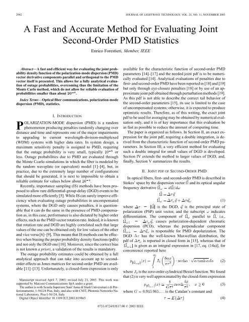
2942 JOURNAL OF LIGHTWAVE TECHNOLOGY, VOL. 21, NO. 11, NOVEMBER 2003 

A Fast and Accurate Method for Evaluating Joint 

Second-Order PMD Statistics 

Abstract—A fast and efficient way for evaluating the joint probability 

density function of the polarization-mode dispersion (PMD) 

vector derivative components parallel and orthogonal to the PMD 

vector itself is presented. This allows for a fully analytical evaluation 

of outage probabilities, overcoming thus the limitation of the 

Monte Carlo method, which do not allow for reliable evaluation of 

probabilities smaller than about IH R . 

Index Terms—Optical fiber communications, polarization-mode 

dispersion (PMD), statistics. 

I. INTRODUCTION 

POLARIZATION-MODE dispersion (PMD) is a random 

phenomenon producing penalties randomly changing over 

distance and time and represents one of the major impairments 

to upgrading to current wavelength-division-multiplexed 

(WDM) systems with higher data rates. In system design, a 

maximum sensitivity penalty is assigned to PMD, requiring 

that the outage probability is very small, typically or 

less. Outage probabilities due to PMD are evaluated through 

the Monte Ccarlo simulations in which the fiber is modeled by 

the random waveplate (or equivalent) model [1]–[4], but, in 

practice, due to the extremely large number of configurations 

that should be generated, it is next to impossible to obtain a 

reliable estimate for values below about . 

Recently, importance sampling (IS) methods have been proposed 

to allow rare differential-group-delay (DGD) events to be 

simulated more efficiently [5]. While IS can surely improve efficiency 

when evaluating outage probabilities in uncompensated 

systems, where the DGD only causes penalties, it is questionable 

that it can do the same in the presence of PMD compensation 

as, in this case, performance is also dictated by higher order 

effects, such as the PMD vector rotation rate. Indeed, it is known 

that rotation rate and DGD are highly correlated such that large 

values of the one can be obtained only for low values of the other 

and vice versa [6]–[9]. This means that IS methods can be effective 

when biasing the proper probability density functions (pdfs) 

and not only the DGD one [10]. Moreover, since the correct bias 

is not known a priori, a validation of the results is mandatory. 

The outage probability estimates could be obtained by a full 

analytical approach that can take into account up to secondorder 

effects as Jones matrices for second-order PMD are available 

[11]–[13]. Unfortunately, a closed-form expression is only 

Manuscript received April 7, 2003; revised July 21, 2003. This work was 

supported by Marconi Communications SpA under a grant. 

The author is with Scuola Superiore Sant’Anna di Studi Universitari e di Perfezionamento, 

1-56124 Pisa, Italy, and also with CNIT, Photonic Networks National 

Laboratory, Pisa I-56124, Italy. 

Digital Object Identifier 10.1109/JLT.2003.819865 

Enrico Forestieri, Member, IEEE 

0733-8724/03$17.00 © 2003 IEEE 

available for the characteristic function of second-order PMD 

parameters [14]–[17] and the needed joint pdf is to be numerically 

evaluated [14]. Analytical evaluations of penalties due to 

first- and second-order PMD have been reported in [18] and [19] 

but only through eye-closure penalties [18] or by use of an approximate 

joint pdf obtained through perturbation methods [19]. 

As this pdf is not able to describe the correct tail behavior of 

the second-order parameters [15], its use is limited to the case 

of uncompensated systems; otherwise, it is expected to produce 

optimistic results. Therefore, as of this writing, the exact joint 

pdf to be used for averaging may be obtained by numerical evaluation 

only, and it is of key importance that this evaluation be 

as fast as possible to reduce the amount of computing time. 

The paper is organized as follows. In Section II, an exact expression 

for the joint pdf, requiring a double integration, is derived 

from the characteristic function of second-order PMD parameters. 

In Section III, a very efficient method for evaluating 

such a double integral for small values of DGD is developed. 

Section IV extends the method to larger values of DGD, and, 

finally, Section V summarizes the results. 

II. JOINT PDF OF SECOND-ORDER PMD 

In optical fibers, first- and second-order PMD is described in 

Stokes’ space by the dispersion vector and its optical angular 

frequency derivative 

where is the DGD, 

(1) 

is the principal state of 

polarization (PSP) unit vector, and the subscript indicates 

differentiation. The component of parallel to , i.e., 

, causes polarization-dependent chromatic 

dispersion (PCD), whereas the perpendicular component 

DGD 

is responsible for PMD depolarization. The 

has the well-known Maxwellian distribution, the 

pdf of is reported in closed form in [15], whereas that of 

is given as an integral expression in [17, eq. (14a)], for 

convenience reported here 

where is the zero-order cylindrical Bessel function. We found 

that (2) is very well approximated by the closed-form expression 

where is the Catalan’s constant and 

(2) 

(3) 

(4)

FORESTIERI: A FAST AND ACCURATE METHOD FOR EVALUATING JOINT SECOND-ORDER PMD STATISTICS 2943 

Fig. 1. Pdf of for a 15-, 20-, and 30-ps mean DGD. Circles are obtained 

from (2), and solid lines from (3). 

where means expectation, is the mean DGD. A comparison 

of (2) and (3) is shown in Fig. 1. 

Even if the pdf of all the quantities appearing in (1) is 

known, this is not enough as, for averaging, the joint pdf 

is needed. 1 As and is known [14], 

we focus on , which is the unknown quantity we need. 

Following [15], we let 

and denote by 

the normalized PMD vector and its derivative, respectively. 

Parameter is the standard deviation of each one of the 

components of the dispersion vector . In the reference frame 

whose first axis is coincident with , the characteristic function 

of the conditional joint pdf 

of the components 2 is [15] 

where 

is the three-dimensional (3-D) transform 

variable and . 

Obtaining a closed-form expression for by analytical 

inversion of (7) proved to be a formidable task, and on the other 

side, a numerical inversion through a 3-D fast Fourier transform 

1For brevity, the pdf arguments are sometimes omitted. 

2In the following ‘1“ denotes transpose. 

(5) 

(6) 

(7) 

(8) 

(FFT) is not feasible as, by simply and optimistically using 64 

points one-dimensional (1-D) FFTs, a total of about 7 000 000 

multiplications should be carried out, which does not exactly 

account for a fast and efficient evaluation. 

Analytical approximations for the joint pdf of and are 

reported in [14] and [15], but, even if second-order moments are 

correctly reproduced, they greatly underestimate the tails 

and therefore are not suitable for PMD-induced penalties evaluation 

in compensated systems. 

Regarding the inversion of (7), as shown in Appendix A, 

after changing to spherical polar coordinates, the 

circular symmetry of one of the angle coordinates allows that 

angle dimension to be easily integrated in closed form, and, 

after a suitable transformation, the joint pdf of and 

, conditional upon , can be written as 3 

where 

(10) 

Hence, to evaluate (9), we have to numerically perform a twodimensional 

(2-D) integral, but a very difficult one, as both 

and the integrand in (10) have an oscillatory nature. 

Indeed, evaluation of through (9) over a grid 

of 100 100 points, covering the tails down to about , 

requires from a few hours to several days of computing time 

on a fast processor, depending on . The higher the value of 

with respect to , the lesser the required time to obtain a 

prescribed accuracy. The inner integral (10) is the most critical 

one, and we tried several numerical integration methods to 

evaluate it, including evaluation through FFT, but the most efficient 

turned out to be a recursive one based on the determination 

of a set of subintervals , , of (0,1) 

such that , , for which 8- and 16-points Gauss 

quadrature formulas give results differing by less than a prescribed 

accuracy . Denoting by , the approximate 

value of the integral on interval given by the -point 

Gauss formula, (10) is approximated as , 

where , for , 

and are found by the following recursive procedure: i) initially 

; ii) for , is successively set to 

, , until the prescribed 

accuracy is attained in ; and iii) the procedure completes 

when accuracy is obtained for . 

III. EVALUATING THE JOINT PDF FOR 

As already pointed out in Section II, the numerical evaluation 

of (9) is not a trivial task. In this section, we will develop a 

method that turns out to be very efficient in the case 

, other than evidencing a key feature of the inner integral 

in (10). 

3 We moved the conditioning on from the subscript to avoid clutter. 

(9)


As shown in Appendix A, the inner integral in (10) 

can be evaluated as 

where is as in (8), whereas 

(11) 

(12) 

Using the first term only in the series expansion (11), we have 

that 

and substituting (13) in (9) yields 

(13) 

(14) 

We will now show that (14) is a good approximation for 

, meaning that very few terms in (11) are needed to approximate 

well when is of the same order as . In order 

to do this, we evaluate the approximate marginals 

and from (14) and compare them with the exact 

ones. To evaluate the marginal pdf , we integrate (14) 

over from to . By performing the change of variable 

, the needed integral can be evaluated with the 

aid of [20, eq. 3.753.3] 

to yield 

(15) 

(16) 

which turns out to be the exact expression for the pdf 

[17]. This means that the approximate pdf (14) is already normalized, 

i.e., it integrates to 1. 

We now evaluate from (14) the marginal pdf 

by integrating over from 0 to . Taking 

into account that the Fourier transform of the unit step function 

is , by the 

change of variable ,wehave 

(17) 

and thus 

from which, as ,wehave 

whereas the exact expression is [15] 

(18) 

(19) 

(20) 

As can be seen, the integrands in (19) and (20) differ by the exponential 

term , but taking into account (8), for 

, it can be approximated with 1 without significantly affecting 

the value of the integral. Therefore, for , the marginals 

obtained from (14) are almost exact, and thus (14) is a good approximation 

to the exact joint pdf. 

A. Evaluating 

In order to use (11), we need an explicit expression for the 

term 

(21) 

and we found several expressions for it. Here, we will use the 

one that we found most convenient from a numerical point of 

view and present a less efficient but simpler alternative in Appendix 

B. 

As shown in Appendix A, (21) can be evaluated through the 

finite sum 

where 

(22) 

(23) 

with being the Kronecker symbol ( if ,0 

otherwise), the integer part of , the Gegenbauer 

polynomial of order and index [21], and 

(24)


which can also be written in a recursive form, more suitable for 

calculation, as 

(25) 

The use of makes evaluation of (23) very efficient because 

Gegenbauer polynomials satisfy the recurrence relation 

[21] 

(26) 

and , for any value of . Therefore, in (23), only 

the polynomial corresponding to should be explicitly 

evaluated, but this can be done, in turn, through the recurrence 

relation [21] 

(27) 

As all quantities appearing in (22) are easily and recursively 

evaluated by performing simple multiplications, it is a very efficient 

expression. As an example, taking into account (26) and 

(27), all the Gegenbauer polynomials needed in (23), for all 

values of , can be obtained with multiplications, at most, 

and only two multiplications need be performed for each to 

evaluate and through (25) as the required values 

for and are to be evaluated only once. Moreover, notice 

that the values in (23) are independent from , and thus they 

need not be reevaluated when performing the outer integral with 

respect to . 

A word of notice is in order here about the correct use of the 

recurrence relation (25). As, for fixed , the sequence 

is decreasing in absolute value with , (25) can be safely used in 

the forward direction for evaluating only when ; 

otherwise, it becomes unstable. Hence, for , (25) is to be 

used in the backward direction 

(28) 

according to the following procedure. As is a decreasing 

function of , for a sufficiently large value of , 

say , the term becomes negligible 

with respect to and can be taken equal to 

zero. Therefore, the starting value to be used with (28) can 

be taken equal to . 

The value of can be readily found in the following 

manner. If is to be evaluated for , 

with , then initially one takes , 

, and applies (28) for 

evaluating . Let us refer 

to the value obtained in this way as . Then, 

the computations are repeated but starting with , 

and the resulting value of is compared with the 

previous one. If their difference is less than a prescribed 

accuracy, say , then 

(28) is repeatedly applied until finding ; 

otherwise one starts again with and so on. We 

found that when choosing , only two iterations are 

required to achieve ten-significant-digits accuracy on . 

Depending on the value of , (28) may lose accuracy for the 

smaller values of ; therefore, for better results, one also uses 

(25) starting from and replacing the corresponding 

values obtained through (28) until their absolute difference 

keeps decreasing. 

For later use, notice that, by using (24) and after some algebra, 

(22) can be written as 

where 

(29) 

(30) 

B. Evaluating the Outer Integral 

The expressions previously developed to evaluate the inner 

integral in (9) turn out to be useful for the evaluation of the outer 

integral, as well. Indeed, in [22], it is shown that integrals of 

the type , where ,as , tends to a form 

that can be written as a steadily decreasing factor times the sum 

of a finite number of sinusoidal terms whose periods tend to 

constant values, can be very efficiently evaluated by means of 

the trapezoidal rule by using a step size close to the shortest 

period . The interval is related to the sampling theorem 

for band-limited functions, and the trapezoidal rule can give the 

exact value of the integral when the step size is less than some 

fixed value [22, p. 709]. 

Taking into account (11), (29), and (30), in (10) can 

be written as 

where 

(31) 

(32)


Fig. 2. @&Y Y A and @&Y Y A in (32) for a aQand 1( a ". Inset 

shows s@&Y Y A in (10) (solid line) and approximation (13) (circles). 

are steadily decreasing functions of , as shown in Fig. 2 for 

and . Thus, the integrand in (9) is of the 

type mentioned previously with , and (9) 

can be efficiently evaluated by the trapezoidal rule as 

(33) 

The sum is stopped when becomes negligible while 

taking the initial step size as 

(34) 

and successively halving it until the result stabilizes in the desired 

number of digits. When halving the step size, the newly 

computed values can be simply added to the trapezoidal sum, 

and the multiplication by the final step size done at the end. We 

found that when taking the initial step size as in (34), in the vast 

majority of cases, it has to be halved only once to achieve fourdigits 

accuracy. By this method, evaluation of 

over the same grid of 100 100 points previously mentioned requires 

only a few tens-of-seconds computing time for , 

with a gain of up to five orders of magnitude with respect to 

the case in which is evaluated through a numerical 

quadrature method. The total number of times that in (33) 

is to be evaluated for four-digits accuracy ranges from , 

for low values of and ,to for the tails down to 

about . Correspondingly, evaluation of through 

(11) requires less than 25 terms, depending on the 

value of , according to the following empirical relation 

, where . In Fig. 3(a) and 

(b), the joint pdf is shown for and 2 , respectively, 

showing that the conditional variance of , 

the normalized component of parallel to , is constant, its 

value being as known [15]. In Fig. 4, , 

evaluated through (33), is plotted for 2 as a function of 

for several values of in (a), and as a function of for several 

values of in (b). Circles represents values obtained through 

numerical integration of (10) as previously explained, whereas 

solid lines are obtained by using (11). 

IV. EVALUATION OF THE JOINT PDF FOR 2 

When the DGD becomes progressively larger than , the 

value of in (8) also increases and a larger number of terms 

would be required to evaluate through (11). This is a 

problem as, when evaluating (21) through (22), the term 

assumes values increasing with and, having the terms in 

(22) alternate signs, this causes too much cancellation for larger 

values of or , preventing evaluation of (21) with the required 

accuracy. We found that evaluation of through (11) 

and (22) is always safe for 2 , but we need alternative 

ways when 2 . 

We discovered several exact expansions for in (10), 

but none of them turned out to be usable for all possible values 

of parameters in (8) and and in (12) without incurring 

in numerical problems similar to those discussed about (22). 

Instead, it is possible to develop an approximate expansion for 

that is always valid whatever the value of , and 

. The key to this expansion is an approximate expansion for 

the term in terms of hyperbolic cosines. We start by 

taking the Fourier transform of , 

where is the unit step function. By completing the square 

in the exponent, the result is formally simple 

(35) 

where is the complex error function. 

We now use an infinite series approximation for the complex 

error function, whose relative error is [21, eq. 7.1.29], 

to write 

and antitransforming back, we obtain 

(36) 

(37) 

with a relative error of for all values of . This means 

that in a double-precision arithmetic (37) is virtually exact. As 

an example, for ,wehave 

double precision 

quadruple precision.


Fig. 3. Joint pdf @Y A for (a) 1( a " and (b) 1( a 2". Contours are at IH , aIY PY FFFY IS. 

By using [21, eq. 10.1.48], we also have that 

(38) 

where are the spherical Bessel 

functions of the first kind. Substituting (37) and (38) in (10), we 

obtain 

where 

(39) 

(40) 

may be evaluated with the aid of [20, eq. 7.322]. 4 By using [21, 

eq. 10.1.45], (39) can be written as 

4 Notice that a factor 2 is missing in the result in [20, eq. 7.322]. 

(41) 

and, taking the principal value, the square root appearing in (41) 

is equal to 

where 

so that (41) becomes 

(42) 

(43) 

(44) 

(45) 

. 

This is the expression to be used for evaluating the joint pdf 

when 2 . Notice that (45) could also be used for 

2 , but, in this case, (11) turns out to be faster. This is because 

in (45) the various elementary functions must be reevaluated for 

each term in the series, whereas (22) only requires the evaluation 

of a few terms through simple recurrence relations, as already 

discussed. For larger values of , however, (11) would require


Fig. 4. Joint pdf @Y A (a) as a function of for 

a RY TY FFFY IT and (b) as a function of for a HY PY FFFY IH and 

1( a 2", evaluated through (33). Circles are obtained through numerical 

integration of (10), solid lines by using (11). 

more terms than those needed in (45), which in most cases are 

in the order of to achieve the necessary precision. Also 

notice that the major contribution does not necessarily come 

from the first terms. Indeed, rewriting (45) as 

(46) 

where , and taking into account that, for increasing 

values of , in (44) asymptotically tends to , 

i.e., , we also have that 

, so that, in many cases, the most important 

terms are those for in the order of , or slightly less. 

Using (45), evaluation of (33) for the larger values of turns 

out to be about an order of magnitude slower than using (11) 

for the smaller values. For the larger values, evaluation 

of (33) through numerical integration of (10) turns out to 

be about an order of magnitude faster than for the smaller 

values. Therefore, using (45) for evaluating (33) is about 

orders of magnitude faster than using the integration method 

described at the end of Section II and even much faster with 

respect to other standard numerical integration methods. However, 

we point out that this discussion applies only when considering 

values for the joint pdf not smaller than about ; 

otherwise standard numerical integration methods slow down 

Fig. 5. Joint pdf @Y A (a) as a function of for 

a RY VY FFFY PV and (b) as a function of for a HY PY RY FFFY IH 

and 1( a 5", evaluated through (33). Circles are obtained through numerical 

integration of (10), and solid lines by using (45). 

considerably, and the values they provide are not reliable (as 

the curves become jagged and sometimes negative values are 

returned), whereas the methods presented in this and Section III 

do not suffer any slow down and can give reliable values down 

to about , i.e., the machine precision in IEEE Standard 

754 double-precision arithmetic. 

In Fig. 5, , evaluated using (45) in (33), is 

plotted for 5 as a function of for several values of in 

(a), and as a function of for several values of in (b). Again, 

circles represents values obtained through numerical integration 

of (10). 

V. SUMMARY AND CONCLUSION 

The exact evaluation of the joint pdf of and , conditional 

upon , can only be performed by numerical methods, 

and, to this end, the double-integral formula (9) has been devised. 

It has been shown that the inner integral (10) has an 

analytic expression that can be exploited for a really efficient 

evaluation of the outer integral in (9) through (33), practically 

equivalent to a series expansion, as the step size (34) is to be 

halved only once in about 90% of cases, on average, to achieve 

four-digits accuracy when evaluating in (10) with sufficient 

accuracy; indeed, the fact that the step size is to be halved 

more than once may be taken as an indication of poor accuracy 

on .


Evaluation of the inner integral in (10) is the most 

critical, as it is to be evaluated with very high accuracy for the 

tails of the joint pdf, and we had to use a value for accuracy 

as small as in the numerical integration method described 

at the end of Section II to obtain reliable values down to 

. We also noticed that the higher the accuracy in evaluating 

, the lesser the number of times that step size 

in (33) is to be halved to achieve a given number of reliable 

digits for the joint pdf. The very high accuracy needed for 

is easily and efficiently achieved through the expansions 

reported in Sections II–IV. Until a closed-form expression 

is not available, a fast and accurate method for evaluating the 

joint second-order PMD statistics is a prerequisite for a full analytical 

evaluation of the PMD impact on the performance of 

compensated systems and may also be a useful tool for validating 

IS techniques (see Appendix C). 

APPENDIX A 

In this appendix, we show the derivation of (9), (11), and (22) 

mentioned in the paper. The exact expression for 

can be obtained by direct antitransformation of (7) as 

(A1) 

where is as in (8). Changing to spherical polar coordinates 

yields 

(A2) 

and the integral with respect to is easily performed, yielding 

(A3) 

From (A3), we obtain the joint pdf of and 

as 

(A4) 

from which, by the change of variable and after some 

algebra, we obtain (9). 

By using the expansion , the integral 

in (10) can be evaluated as 

Letting and as in (12), we start from [20, eq. 6.677.6] 

and, by repeated differentiation with respect to , obtain 

(A5) 

(A6) 

(A7) 

which, substituted in (A5), gives (11). 

Thus, we simply need an explicit expression for the 

right-hand-side term in (A7). To obtain it, we use the rule 

for the th derivative of a composite function. Letting 

(such that ), if 

, then [20] 

where 

(A8) 

(A9) 

Given , where 

, , we apply the previous rule 

to obtain the th derivative of as 

where 

By using the formula [20] 

(A10) 

(A11) 

(A12) 

where denotes the Pochhammer’s symbol, defined as [21] 

(A13)


being the Gamma function, it is easy to show that 

(A14) 

in which we can recognize the Gegenbauer polynomial of order 

and index as 

so that 

(A15) 

(A16) 

Letting and substituting (A16) in (A11), we obtain 

(A17) 

where we made the change of variable . Taking now 

into account the fact that 

(A17) can also be written as 

and substituting (A19) in (A10), we obtain (22). 

(A18) 

(A19) 

APPENDIX B 

As already said, we found several different expansions for 

evaluating (21), and in this appendix, we report the one that 

turned out to be the most competitive with (22). Thus, somewhat 

sacrificing performance, it could be used as an alternative to 

(22). For the sake of brevity, we will only report a trace of the 

full proof. 

It is easy to show that the relation [21, eq. 10.1.24] 

also holds for 

i.e., 

and, using (B3), by induction, we have 

. . . 

. 

.. 

Taking now into account that 

, we obtain 

(B1) 

(B2) 

(B3) 

(B4) 

The spherical Bessel functions needed in (B4) can be efficiently 

evaluated by a simple recurrence relation [21] or through 

one of the many available subroutines for evaluating the cylindrical 

functions of fractional order . Although more compact 

than (22), we found that (B4) is less efficient than it when 

used in (11) for evaluating (33). 

APPENDIX C 

A fast and accurate method for the evaluation of the joint pdf 

is also useful for validating other techniques used for outage 

probabilities estimation. In this appendix, we apply the methods 

previously developed to evaluate the joint pdf of and 

and compare it with the joint pdf obtained numerically through 

IS in [10] and [23]. 

As known [24], the joint pdf of and5 , where and have joint pdf , 

is , and the marginal pdf 

for can be obtained as . Therefore, 

5 The —— function is taken to return values between 0 and %.


letting , , and taking into account (9), it can 

be shown that 

where 

(C1) 

(C2) 

(C3) 

By the change of variable and using [20, eq. 6.677.6], 

in (C3) can be integrated in closed form, and we see that it is 

independent from 

Substituting (C4) in (C2) and, in turn, this in (C1), we obtain 

where 

(C4) 

(C5) 

(C6) 

is as in (45) for , i.e., . Multiplying 

(C5) by the Maxwellian pdf finally gives 

(C7) 

where the integral can be evaluated as done in (33) with an initial 

step size of . 

Fig. 6 shows contour plots of the denormalized joint pdf 

(C8) 

for 3.257 ps, evaluated through (C7), and should be 

compared with Fig. 4 in [23], reporting the same quantity at the 

Fig. 6. Contour plots of the joint pdf of and for a mean DGD of 

3.257 ps. Starting from the inner, the contours are at IH with a 1.5, 1.75, 

2, 2.25, 2.5, 3, 4, 5, 6, 8, 10, 15, 20, 25, and 30. 

same contour levels. A close examination reveals that the accordance 

is excellent until , but afterwards, the joint pdf 

obtained through IS starts underestimating the true pdf progressively 

more as the contour level lowers. The contours below 

in Fig. 6 required quadruple precision to be computed 

(notice that (C6) can be used for values smaller than when 

using a higher precision arithmetic, but only about the first 16 

significant digits are correct). 

REFERENCES 

[1] C. D. Poole and D. L. Favin, “Polarization-mode dispersion measurements 

based on transmission spectra through a polarizer,” J. Lightwave 

Technol., vol. 12, pp. 917–929, June 1994. 

[2] D. Marcuse, C. R. Menyuk, and P. K. Wai, “Application of the manakov-PMD 

equation to studies of signal propagation in optical fibers 

with randomly varying birefringence,” J. Lightwave Technol., vol. 15, 

pp. 1735–1746, Sept. 1997. 

[3] R. Khosravani Jr, I. T. Lima, P. Ebrahimi, E. Ibragimov, A. E. Willner, 

and C. R. Menyuk, “Time and frequency domain characteristics of polarization-mode 

dispersion emulators,” IEEE Photon. Technol. Lett., vol. 

13, pp. 127–129, Feb. 2001. 

[4] A. O. Dal Forno, A. Paradisi, and J. P. von der Weid, “Experimental and 

theoretical modeling of polarization-mode dispersion in single-mode 

fibers,” IEEE Photon. Technol. Lett., vol. 12, pp. 296–298, Mar. 2000. 

[5] G. Biondini, W. L. Kath, and C. R. Menyuk, “Importance sampling for 

polarization-mode dispersion,” IEEE Photon. Technol. Lett., vol. 14, pp. 

310–312, Mar. 2002. 

[6] B. L. Heffner, “Accurate, automated measurement of differential group 

delay dispersion and principal state variation using Jones matrix eigenanalysis,” 

IEEE Photon. Technol. Lett., vol. 5, pp. 814–817, July 1993. 

[7] L. M. Gleeson, E. S. R. Sikora, and M. J. O. Mahoney, “Experimental 

and numerical investigation into the penalties induced by second order 

polarization mode dispersion at 10 Gb/s,” in Proc. ECOC’97, vol. 1, 

1997, pp. 15–18. 

[8] D. Penninckx and F. Bruyère, “Impact of the statistics of second-order 

polarization-mode dispersion on systems performance,” in OFC’98 

Tech. Dig., 1998, Paper ThR2, pp. 340–342. 

[9] L. E. Nelson, R. M. Jopson, H. Kogelnik, and G. J. Foschini, “Measurement 

of depolarization and scaling associated with second-order polarization 

mode dispersion in optical fibers,” IEEE Photon. Technol. Lett., 

vol. 11, pp. 1614–1616, Dec. 1999. 

[10] S. L. Fogal, G. Biondini, and W. L. Kath, “Multiple importance sampling 

for first- and second-order polarization-mode dispersion,” IEEE Photon. 

Technol. Lett., vol. 14, pp. 1273–1275, Sept. 2002. 

[11] A. Eyal, W. K. Marshall, M. Tur, and A. Yariv, “Representation of 

second-order polarization mode dispersion,” Electron. Lett., vol. 35, 

no. 19, pp. 1658–1659, 1999. 

[12] H. Kogelnik, L. E. Nelson, J. P. Gordon, and R. M. Jopson, “Jones matrix 

for second-order polarization mode dispersion,” Opt. Lett., vol. 25, no. 

1, pp. 19–21, 2000.


[13] E. Forestieri and L. Vincetti, “Exact evaluation of the jones matrix of a 

fiber in the presence of polarization mode dispersion of any order,” J. 

Lightwave Technol., vol. 17, pp. 1898–1909, Dec. 2001. 

[14] G. J. Foschini and C. D. Poole, “Statistical theory of polarization 

dispersion in single mode fibers,” J. Lightwave Technol., vol. 9, pp. 

1439–1456, Nov. 1991. 

[15] G. J. Foschini, R. M. Jopson, L. E. Nelson, and H. Kogelnik, “The statistics 

of PMD-induced chromatic fiber dispersion,” J. Lightwave Technol., 

vol. 17, pp. 1560–1565, Sept. 1999. 

[16] G. J. Foschini, L. E. Nelson, R. M. Jopson, and H. Kogelnik, “Probability 

densities of second-order polarization mode dispersion including polarization 

dependent chromatic fiber dispersion,” IEEE Photon. Technol. 

Lett., vol. 12, pp. 293–295, Mar. 2000. 

[17] , “Statistics of second-order PMD depolarization,” J. Lightwave 

Technol., vol. 19, pp. 1882–1886, Dec. 2001. 

[18] F. Bruyére, “Impact of first- and second-order PMD in optical digital 

transmission systems,” Optic. Fiber Technol., vol. 2, pp. 269–280, 1996. 

[19] H. Bülow, “System outage probability due to first- and second-order 

PMD,” IEEE Photon. Technol. Lett., vol. 10, pp. 696–698, May 1998. 

[20] I. S. Gradshteyn and I. M. Ryzhik, Table of Integrals, Series, and Products. 

San Diego, CA: Academic, 1992. 

[21] M. Abramowitz and I. A. Stegun, Handbook of Mathematical Functions. 

New York: Dover, 1972. 

[22] S. O. Rice, “Efficient evaluation of integrals of analytic functions by 

the trapezoidal rule,” Bell Syst. Tech. J., vol. 52, no. 5, pp. 707–722, 

May–June 1973. 

[23] S. L. Fogal, G. Biondini, and W. L. Kath, “Multiple importance sampling 

for first- and second-order polarization-mode dispersion,” IEEE Photon. 

Technol. Lett., vol. 14, p. 1487, Oct. 2002. 

[24] A. Papoulis, Probability, Random Variables, and Stochastic Processes. 

New York: McGraw-Hill, 1991. 

Enrico Forestieri (S’91–M’92) was born in Milazzo, Italy, in 1960. He received 

the Dr. Ing. degree in electronics engineering from the University of Pisa, Pisa, 

Italy, in 1988. 

From 1989 to 1991, he was a Postdoctoral Scholar at the University of Parma, 

Parma, Italy, working in optical communication systems. From 1991 to 2000, 

he was a Research Scientist and Faculty Member of the University of Parma. 

He is now Associate Professor of Telecommunications at the Scuola Superiore 

Sant’Anna, Pisa, Italy. His research interests are in the area of digital communication 

theory and optical communication systems.

A fast and accurate method for evaluating joint second-order PMD ...

You also want an ePaper? Increase the reach of your titles

Delete template?

Save as template?